Introduction
Biological activity in soil varies with water content, soil texture and structure, temperature, energy and nutrient resources, and species composition (Coleman et al. Reference Coleman, Crossley Jr and Hendrix2004). The effect of water is usually expressed as a function of matric potential (Griffin Reference Griffin1981), although other measures such as the fraction of water-filled pore space (Linn & Doran Reference Linn and Doran1984) and volumetric water (West et al. Reference West, Sparling, Feltham and Reynolds1992) have been employed. Soil water potential has several components including matric, osmotic, pressure and gravitational potentials. Matric potential, resulting from physical forces between water and soil particles, is the most important determinant of biological activity under most natural conditions, except in salty soils where the osmotic component also must be considered (Griffin Reference Griffin1981).
A variety of mathematical equations has been used to describe the relationship between soil water content and matric potential. Many published equations are semi-empirical, with some parameters related to physically measurable soil properties and other parameters (fitted parameters) adjusted to achieve a good fit to data (Clapp & Hornberger Reference Clapp and Hornberger1978, McCuen et al. Reference McCuen, Rawls and Brakensiek1981, Vereecken et al. Reference Vereecken, Maes, Feyen and Darius1989). Water-retention equations (WREs) have been adapted to soils with different bulk properties (e.g. texture, bulk density, organic matter content) by either using regression analysis to relate parameter values to soil properties, or specifying different parameter values for different textural classes. Models of the second sort implicitly assume that variation within a textural class is unimportant. The empirical nature of most WREs is reflected in their failure to represent one or more fundamental characteristics of water-retention data, for example that water content equals the saturation level at zero matric potential.
We required a WRE for use in studies of biological activity in soils of the McMurdo Dry Valleys of Antarctica. Most of the soil water data available from the Dry Valleys (e.g. Vishniac Reference Vishniac and Friedmann1993, Freckman & Virginia Reference Freckman and Virginia1997, Treonis et al. Reference Treonis, Wall and Virginia1999, Courtright et al. Reference Courtright, Wall and Virginia2001, Porazinska et al. Reference Porazinska, Wall and Virginia2002, Parsons et al. Reference Parsons, Barrett, Wall and Virginia2004) are reported as gravimetric water, which should be converted to matric potential for the most accurate prediction of organism activity (Griffin Reference Griffin1981, Killham Reference Killham1994, Hunt et al. Reference Hunt, Wall, DeCrappeo and Brenner2001). The Dry Valleys are cold deserts with an annual precipitation less than 10 cm (Fountain et al. Reference Fountain, Lyons and Burkins1999); thus, a useful equation must perform well in dry soil. Because there are few moisture release data available for Antarctic soils, we required a theoretically sound equation to minimize the number of parameters that must be estimated from data. Dry Valley soils generally are sandy, poorly weathered and poorly structured (Campbell & Claridge Reference Campbell and Claridge1987), with extremely low organic matter contents (0.02–0.08%, Campbell Reference Campbell2003) and with poorly weathered clay minerals (Pastor & Bockheim Reference Pastor and Bockheim1980). Soils with distinctive properties from geographical regions such as the Dry Valleys may require special WREs (Wösten et al. Reference Wösten, Pachepsky and Rawls2001). The objective of the present research was to develop a WRE that is applicable to sandy soils with low organic matter content, requires a minimal number of parameters estimated from data, requires minimal information on texture (sand, silt and clay only), and correctly represents the fundamental characteristics of water-retention curves.
Literature
We evaluated several WREs that have been applied to sandy soils (here denoting USDA sand and loamy sand textural classes). The first equation is a simple power curve (Clapp & Hornberger Reference Clapp and Hornberger1978):

where θ is volumetric water content (cm3 water per cm3 dry soil), θs is water content at saturation, ψ is matric potential (kPa), ψs is matric potential at saturation (air entry potential) and b is a “fitting parameter” (adjusted to achieve a fit to data). Clapp & Hornberger (Reference Clapp and Hornberger1978) used a modified version of Eq. (1) to represent variation in water-retention data among soil textural classes by assigning values for parameters θs, ψs and b for each of eleven textural classes, for a total of more than 33 fitted parameters. The second equation is a version of the van Genuchten (Reference van Genuchten1980) equation recommended by Vereecken et al. (Reference Vereecken, Maes, Feyen and Darius1989):

where θr is residual (minimal) volumetric water (cm3 water per cm3 dry soil), α and η are parameters, and other variables are defined as above. Vereecken et al. (Reference Vereecken, Maes, Feyen and Darius1989) fitted Eq. (2) to data for different soils by deriving regression equations for the four parameters (θs, θr, α and η) as functions of bulk density, sand, silt, clay and organic matter content, with a total of 15 fitted coefficients. The third equation (Brooks & Corey Reference Brooks and Corey1964) is:

where λ is a parameter, and other variables are defined as above. Equation (3) is similar to Eq. (1), but with the addition of a parameter for residual water. McCuen et al. (Reference McCuen, Rawls and Brakensiek1981) estimated values for the four parameters of Eq. (3) (θs, θr, λ and ψs) for each of eleven textural classes, for a total of 44 fitted parameters. The fourth equation, based on the “additivity hypothesis” (Zeiliguer et al. Reference Zeiliguer, Pachepsky and Rawls2000), is:

Equation (4) differs fundamentally from Eqs (1–3) in that some soil properties (sand, silt and clay fractions; bulk density) are incorporated directly into the structure of the equation, rather than being related statistically via fitting parameters. The three terms on the right-hand side of Eq. (4) represent water associated with the sand, silt and clay fractions as a function of matric potential ψ. Variables ft and fc are the mass fractions of silt and clay, respectively, in dry soil, and bd is bulk density (g dry soil per cm3). Operator exp(x) denotes ex, where e is the base of natural logarithms. There are eight fitting parameters: wt and wc are gravimetric water (g water per g dry soil) in silt and clay, respectively, at saturation, and ms, hs, mt, ht, mc and hc (with s, t and c denoting sand, silt or clay) determine the shape of the curves relating water content to ψ for the three particle size fractions.
Parameters in models based on Eqs (1) & (3) took distinct values for each textural class (in the analyses of Clapp & Hornberger (Reference Clapp and Hornberger1978) and McCuen et al. (Reference McCuen, Rawls and Brakensiek1981), and thus these models did not predict variation of water-release curves within classes. Models based on Eqs (2) & (4) allowed for continuous variation between and within textural classes. The four equations differ in their performance at extreme water contents. For example, Eqs (1) & (3) assign a matric potential ψ less than zero (ψs) at saturation water content θs, while Eqs (2) & (4) assign a value of zero, as appropriate from the definition of water saturation. As ψ approaches -∞, volumetric water θ approaches a non-zero residual level (θr) according to Eqs (2) & (3), but approaches zero according to Eqs (1) & (4).
Assuming saturation water content equals total porosity, θs is related to soil bulk density bd according to

where sg is the particle density of solid soil constituents. The equating of porosity and saturated water content has been applied across a range of soil textures (Cosby et al. Reference Cosby, Hornberger, Clapp and Ginn1984). θs in Eq. (4) is calculated using Eq. (5). For Eq. (3), McCuen et al. (Reference McCuen, Rawls and Brakensiek1981) calculated porosity from bulk density and particle density, presumably according to Eq. (5). For Eq. (2) (Vereecken et al. Reference Vereecken, Maes, Feyen and Darius1989), θs was predicted from a multiple regression equation in which θs declined linearly with increasing bd. For Eq. (1), θs was estimated for each water-release curve to maximize fit to data, without reference to bd (Clapp & Hornberger Reference Clapp and Hornberger1978). Assuming that θs declines with increasing bd, then models based on Eqs (1) & (3) predict that θ decreases as bd increases in dry as well as in wet soil, for a given texture. To the contrary, θ in dry soil (for a given texture and matric potential) should be directly proportional to bd, assuming that water in dry soil is mainly adsorbed to particle surfaces and held at interstices between adjacent particles, because there are more soil particles per unit volume at higher bd. Such a relationship is supported empirically (Siegel-Issem et al. Reference Siegel-Issem, Burger, Powers, Ponder and Patterson2005). In the Vereecken et al. (Reference Vereecken, Maes, Feyen and Darius1989) application of Eq. (2), θ increases with bd at intermediate water contents, but the effect of bd is too large (greater than proportionality) at intermediate water contents, and the effect disappears in dry soil as θ approaches θr. Several other models in the literature incorporate effects of bd in addition to that in Eq. (5). Campbell (Reference Campbell1985) expressed ψs in Eq. (1) as an increasing function of bulk density, but the resulting model fails to predict that θ increases with bd in dry soil. Winfield (Reference Winfield2005) applied a WRE (Rossi & Nimmo Reference Rossi and Nimmo1994) with three different functional forms for different regions of the water-release curve. Parameters of the WRE were predicted from regression equations as functions of bulk density and particle-size distributions. Because the equations are complicated, we evaluated them numerically for the sandiest set of soils (the third dataset in Winfield's table 3). Again, θ in dry soil failed to increase with bd.
Materials and methods
Data employed
We found only two studies which provided texture and water-release data for Antarctic Dry Valley soils, and which employed standard particle size definitions. The first is an unpublished part of a study of nematode activity and abundance in McMurdo Dry Valleys (Treonis et al. Reference Treonis, Wall and Virginia1999, Reference Treonis, Wall and Virginia2000, Reference Treonis, Wall and Virginia2002). Soil collected from the upper 10 cm near Lake Hoare, Taylor Valley, was sieved to remove particles larger than 2 mm. Soil structure was not preserved by this sampling procedure, but Dry Valley soils generally have no cohesive structure due to high sand and low organic content, and frequent freeze-thaw cycles (Campbell & Claridge Reference Campbell and Claridge1987). A tension plate apparatus (Klute Reference Klute and Klute1986) was used to manipulate soil water content over a range of high potentials (0, -1, -2.5, -5, -8.8 kPa). Soil was packed into soil-retaining rings and wetted to saturation on ceramic plates so that the curve obtained represents the drying curve. After 24 h equilibration at saturation, suction was applied. Soil moisture was determined gravimetrically (24 h at 105°C) after at least 24 h equilibration at each suction level. Soil texture (95.7% sand, 1.8% silt, 2.5% clay) was determined by the hydrometer method (Gee & Bauder Reference Gee, Bauder and Klute1986). Bulk density (1.67) was determined by packing dry soil into a container of known volume. The second study (Ugolini Reference Ugolini1963) employed soils from a profile (2–6, 6–15, 15–25, 25–30, and 30–37 cm) in the Wright Valley, Antarctica. Samples were sieved to remove particles greater than 2 mm, leached to remove salts, and exposed to atmospheres with relative humidity regulated to either 98.2% (-2499 kPa, assuming tests were at 25°C) or 50.0% (-95 361 kPa).
The above two studies from the Dry Valleys cover the wet and dry ends of the water-release curve. A third study (Rivers & Shipp Reference Rivers and Shipp1978) was not of Dry Valley soils, but employed samples “from soil profiles developed in materials deposited by glacial melt waters” in North Dakota. Samples were taken from below the surface horizons to minimize organic matter. Five particle sizes within the sand category were given, and average sand diameter ranged from 0.14 to 0.55 mm. A pressure plate apparatus was used to set potentials to -5.0, -6.7, -10. and -1500 kPa, which bridge the gap between the first two datasets. Bulk densities were determined from field samples, and varied from 1.47 to 1.59.
We were unable to fit Eq. (4) to all three datasets using a single set of parameters, because the samples at -2500 kPa (Ugolini Reference Ugolini1963) had too high a water content in relation to their clay content compared to the samples at -1500 kPa (Treonis unpublished). The explanation for the discrepancy may lie in the use of different methods for manipulating soil water content suction plates by Treonis, pressure plates by Rivers & Shipp (Reference Rivers and Shipp1978), and control of atmospheric humidity by Ugolini (Reference Ugolini1963). Only the humidity method is sensitive to soluble salts, which increase water content for a given total (matric + osmotic) potential. Data for leached soils only were used from the Ugolini study, but he did not describe the leaching method or present evidence of its efficacy. Thus soil salinity cannot be ruled out as an explanation for high water contents (relative to soil clay) in the Ugolini data. The suction plate method (Treonis data), in contrast, produced low soil water contents relative to matric potential and clay content. Entrapped air (Sakaguchi et al. Reference Sakaguchi, Nishimura and Kato2005) is a possible explanation for anomalously low θ values at high potentials. We selected the Rivers & Shipp (Reference Rivers and Shipp1978) data for model development because 1) these samples shared properties - glacial origin, low organic matter, high sand (82–96%) and low clay contents (2.3–6.6%) - with most Dry Valley soils, 2) these data appeared to suffer from fewer technical problems than the Dry Valley samples, and 3) the data included the widest range of soil textures and matric potentials.
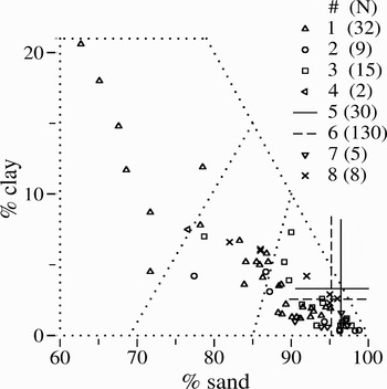
Figure 1 shows the distribution of soil textures of the samples used for model development, and of published data from the McMurdo Dry Valleys and other Antarctic ice-free areas. Textures were about 90% sand class, 6% loamy sand and 3% sandy loam. The Rivers & Shipp (Reference Rivers and Shipp1978) samples used for model development approximated the distribution of Antarctic soil textures, but differed in the absence of sandy loam soils, most of which were from ice free areas other than the McMurdo Dry Valleys, and in having slightly greater ratios of clay to sand.
Soil textures of samples from Antarctic ice-free areas and of samples used for model development. Three regions of the graph separated by dotted lines are for sandy loam, loamy sand, and sand textures (USDA definitions), left to right. The legend gives source of data (#) and sample size (N). Sources are #1 (Claridge & Campbell Reference Claridge and Campbell1968), #2 (Claridge Reference Claridge1965), #3 (Pastor & Bockheim Reference Pastor and Bockheim1980), #4 (Ugolini & Anderson Reference Ugolini and Anderson1973), #5 (Parsons et al. Reference Parsons, Barrett, Wall and Virginia2004), #6 (Freckman & Virginia Reference Freckman and Virginia1997) and #7 (Ugolini Reference Ugolini1963), and #8 (Rivers & Shipp Reference Rivers and Shipp1978, used for model development). Data from sources 5 & 6 are presented as ranges including the mean ± two standard deviations, which should include about 95% of observations. Sample locations included the Dry Valleys (sources #2–7), ice-free ground in the Shackleton Glacier Region, Antarctica (source #1), and North American glacial deposits (source #8). Antarctic samples were of variable thickness, but all were from above 13 cm depth. All samples were sieved to exclude particles larger than 2 mm.

Parameter estimation
Volumetric water θ was taken as the dependent variable in Eqs (1–4) to facilitate comparison among equations. However, for purposes of fitting the equations to data, we treated matric potential ψ as dependent variable (a function of θ, soil properties, and parameters) because in the field θ is more easily and reliably measured than ψ. Equations (1–3) were algebraically inverted to solve for ψ. Equation (4) was solved numerically for ψ in order to treat it as the dependent variable.
Some of the parameters in Eq. (4) were taken from the Zeiliguer et al. (Reference Zeiliguer, Pachepsky and Rawls2000) model, and others (fitted parameters identified below) were estimated to minimize E, the sum of squared errors in the natural logarithm of potential:

where ψm is matric potential predicted by Eq. (4) as a function of observed θ, ψd is observed matric potential, and the summation is over 31 observations (eight soil samples times four potentials minus one missing observation). The logarithm transformation was chosen on the assumption that measurement errors of potential were proportional to the absolute value of potential. The added constant (0.1) prevents undefined logarithms in case ψ = 0. The dependent variable (-ψm + 0.1) varied over almost five orders of magnitude. Minimization of E was accomplished by augmented SIMPLEX optimization (Hunt et al. Reference Hunt, Antle and Paustian2003).
Several alternative models also were fitted to the data. Equation (2) was fitted by retaining the original regression equations for parameters (θr, θs, α and η) as a function of texture, bulk density and carbon content (Vereecken et al. Reference Vereecken, Maes, Feyen and Darius1989, first entries in their table 7), but adjusting each parameter value by a multiplier estimated to minimize error according to Eq. (6). A modified version of Eq. (2) was fitted to the data by setting θr to zero and estimating multipliers for the remaining three parameters to minimize error. We modified Eq. (3) to predict continuous variation in water-release curves within sandy soils by using the Vereecken equations for parameters θr and θs (see above), and estimated parameters ψs and λ to minimize error. Another modified version of Eq. (3) (equivalent to Eq. (1)) was fitted by setting θr to zero, and estimating the remaining parameters as explained above.
Results
Development of new water-release equation
Equation (4) is derived from a model (Zeiliguer et al. Reference Zeiliguer, Pachepsky and Rawls2000) based on the additivity hypothesis, according to which experimentally determined water-release curves for nine individual soil particle size fractions (0–0.001, 0.001–0.005, … , 0.5–1, 1–3 mm) contribute to the release curve of a whole soil in proportion to the mass of each size fraction in the whole soil. We could not apply the Zeiliguer et al. (Reference Zeiliguer, Pachepsky and Rawls2000) model directly because most texture data available for Dry Valley soils distinguish only three particle size fractions. Thus we simplified the Zeiliguer model by reducing the number of soil fractions from nine to three (sand, silt and clay). In Eq. (4), the “h” parameters (hs, ht and hc for sand, silt and clay, respectively) are the matric potentials at which water associated with a size fraction ≈ 36.8% (1/e) of its saturation value. The “m” parameters (ms, mt and mc) determine how abruptly water associated with a size fraction changes with ψ, when ψ equals the corresponding “h” parameter.
Saturation water (θs) in Eq. (4) was predicted from bulk density bd according to Eq. (5), using a value of 2.75 g cm-3 for particle density sg. Vereecken et al. (Reference Vereecken, Maes, Feyen and Darius1989), treating the whole spectrum of soil textures, included an effect of clay on θs, but according to their model the clay effect would be insignificant in sandy soils. The value usually assumed for sg (e.g. Cosby et al. Reference Cosby, Hornberger, Clapp and Ginn1984) is 2.65, that of quartz. Campbell & Claridge (Reference Campbell and Claridge1987) reported orthoclase, oligoclase, biotite, quartz and hornblende as common minerals in Dry Valley soils. The particle density of these minerals ranges from 2.55 to 3.45. We found that the fit of the model to data was not very sensitive to the value of sg, and arbitrarily assigned an intermediate value of 2.75.
Parameter wt in Eq. (4) (g water per g silt at saturation) was set to 0.30, the average for two silt fractions of the corresponding parameter (Wi,0, with i indicating particle size fraction) in the Zeiliguer et al. (Reference Zeiliguer, Pachepsky and Rawls2000) model. Parameter wc was estimated to achieve the best fit to data, and its value (0.92 g water per g dry clay) was within the range (0.31–0.92) of Zeiliguer model parameter Wi,0 for their two clay size fractions. The Zeiliguer model parameters Wi,0 for five sand size fractions varied from 0.24 to 0.27 g water per g dry sand, but there is no corresponding parameter in Eq. (4) (see discussion below).
Zeiliguer et al. (Reference Zeiliguer, Pachepsky and Rawls2000) employed a double Weibull equation with seven parameters for the release curve of each of nine particle size fractions. We reduced the number of parameters by using a single Weibull equation for each of three size fractions (see Eq. (4)). We eliminated the Zeiliguer parameter for residual water (by setting θr = 0), on the assumption that soil water will approach zero if matric potential falls low enough. The single Weibull “h” parameters (as in Eq. (4) for each of the nine particle size fractions in Zeiliguer et al. (Reference Zeiliguer, Pachepsky and Rawls2000) were estimated by numerically evaluating their double Weibull. The resulting h values (kPa) for their seven sand and silt fractions were regressed on the mid point d (mm) of the particle size range:

The form of Eq. (7) is theoretically appropriate (cf. eq. (4) in Haverkamp & Parlange Reference Haverkamp and Parlange1986). Equation 7 accounted for 98.5% (P < .0001) of the variation in ln(-h), and was used to estimate hs for the sand fraction in Eq. (4), with d equal to mean particle size for the sand fraction. For a nominal sand diameter of 0.28 mm, hs takes a value of -3.9 kPa. Values of “h” for silt (ht = -230 kPa) and clay (hc = -4250 kPa) were estimated to achieve the best fit to data. The relative values of “h” parameters ensure that sand-associated water is lost first as a soil dries, followed by water associated with silt and clay fractions. The “m” parameters of Eq. (4) could not be directly estimated from corresponding Zeiliguer model parameters, because smaller values of “m” are required to achieve a smooth water-release curve when using fewer particle size fractions (three in Eq. (4) vs. nine in the Zeiliguer model). Thus mt for silt and mc for clay were assigned values of 1.0 and 0.5 (non-dimensional), respectively. Parameter md for sand was estimated (1.35) to achieve the best fit to the data.
Zeiliguer et al. (Reference Zeiliguer, Pachepsky and Rawls2000) adjusted their nine Wi,0 parameters (i =1,9; five for sand fractions, plus two each for silt and clay fractions) so that the observed capillary water at saturation in a whole soil (θs) equalled the sum of saturated capillary water associated with each size fraction, weighted by the dry weight fraction fi of each size class in the whole soil:

where W′i,0 is the adjusted value and n = 9. This adjustment was done keeping the ratios of W′i,0 parameters among the nine size fractions the same as the ratios of the Wi,0 parameters determined for individual fractions. In other words, the amounts of saturated water associated with the unmixed size fractions were assumed to keep the same ratios after being mixed together in whole soil. We tried this adjustment method in an earlier version of Eq. (4) which included a parameter ws for capillary water associated with sand at saturation; that is, ws, wt, and wc were adjusted similarly to Eq. (8) with n = 3. The problem with this method of adjusting ws, wt, and wc, was that θ in dry soil inappropriately decreased with increasing bulk density. Zeiliguer et al. (Reference Zeiliguer, Pachepsky and Rawls2000) pointed out that their method (Eq. (8)) of adjusting pore spaces associated with different particle size fractions neglects the likelihood that finer soil particles occupy spaces between larger particles and thus reduce the relative contribution of larger pore spaces. We represented the packing of small particles among larger particles by assuming that large pore space (numerator of first term of Eq. (4)) equals total pore space θs minus pore space associated with silt (ft · wt · bd) and clay (fc · wc · bd). With this assumption and the use of Eq. (5) for θs, Eq. (4) correctly predicts that θ in dry soil increases proportionately with increasing bulk density. We are not aware of any other water-release models with this property.
Fit of models to data
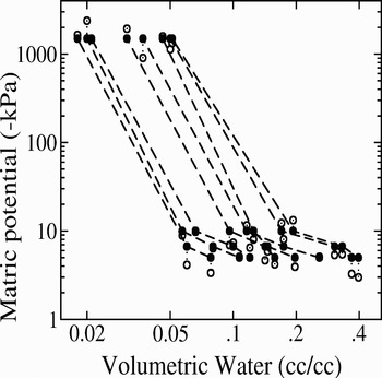
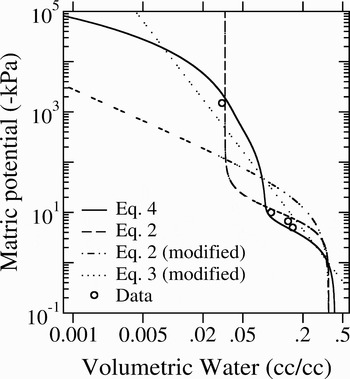
Our model accounted for 98.7% (R 2 = 0.987) of the variation in ln(-ψd + 0.1). Figure 2 shows water-release curves and model errors. Most of the variation among these water-release curves is related to clay content, which increases left-to-right among the curves in the figure. Alternative models with θr≠0 (Eqs (2) & (3)) also fit the data well, with R 2 of 97.7% and 99.4% respectively, but θr values ranged from 0.03 to 0.06, well above the minimal values of 0.1–0.3% reported by Ugolini (Reference Ugolini1963) for Dry Valley soils. When θr was set to zero and the equations refitted to data, R 2 declined to 82% for Eq. (2) and to 87% for Eq. (3), and both models consistently overestimated matric potential at an observed potential of -1500 kPa. Figure 3 compares the shapes of equations, and illustrates how setting θr to zero degrades the fit of Eqs (2) & (3).
Water-release curves for the eight soil samples (Rivers & Shipp Reference Rivers and Shipp1978) used in model calibration. Data (filled symbols) for a given soil sample at different potentials are connected by dashed lines. Predictions of the model (Eqs (4, 5 & 7)) are denoted by open symbols, which are connected to the corresponding data points by dotted lines.

Water-release curves (lines) for Eqs (2–4) and for equations modified by setting θr to zero (see text). Open circles are data for one of the soil samples of Rivers & Shipp (Reference Rivers and Shipp1978), included to indicate the range of matric potential in the data.

To determine the importance of soil properties for the fit of Eq. (4) to data, variation among soils was eliminated by replacing property values for each soil sample with the mean value over all eight samples. When texture of every soil was replaced with mean texture (90.5% sand, 4.4% clay), R 2 declined from 98.7% to 70%. Similarly, R 2 was reduced to 98.5% when using mean bulk density (1.54 g cm-3), to 96.1% using average sand diameter (0.28 mm), and to 70% when all soil properties simultaneously were set to their means. The residual 70% of variation accounted for by the model with constant soil properties results from within sample effects of variable water content on potential.
Effect of bulk density
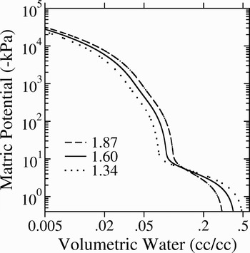
Figure 4 shows the predicted effects of bulk density in a hypothetical soil with 90.5% sand, 4.4% clay, and average sand diameter of 0.28 mm. At high matric potentials near saturation, θ decreases with increasing bd in accordance with Eq. (5). At lower potentials (< -10 kPa), (θ is directly proportional to bd. The crossing point for any two curves of different bd is about -5.4 kPa, not far from the approximate range of -0.1 to -5 kPa given for the crossing point by Siegel-Issem et al. (Reference Siegel-Issem, Burger, Powers, Ponder and Patterson2005) for three sandy loams and a silt loam. Matric potential for a given volumetric water may vary with bd by a factor of ten or more over the range of bd indicated in Fig. 4. In contrast, matric potential for a given gravimetric water (g water per g dry soil) and soil texture is virtually independent of bd in dry soil (Siegel-Issem et al. Reference Siegel-Issem, Burger, Powers, Ponder and Patterson2005). This can be seen from Eq. (4) by setting the first term for sand-associated water to zero, and dividing both sides of the equation by bd (gravimetric water = θ/bd). Thus it is unnecessary to know bd to estimate matric potential from gravimetric water in dry soil.

Effects of texture
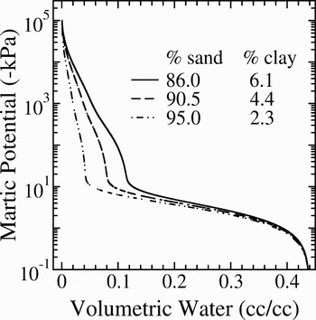
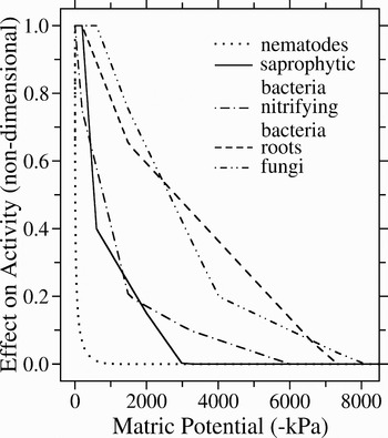
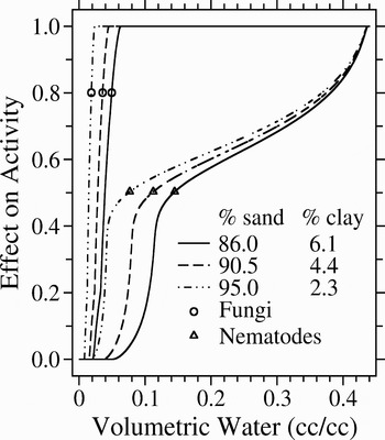
Figure 5 shows the predicted effects of texture over the range of textures in the calibration data (cf. Fig. 2), but extrapolated over a wider range of matric potential and water content. Water contents were very similar at high matric potentials, because all three soils were assigned the same bulk density (1.54). However, at 5% volumetric water, potentials varied from a low of about -1500 to a high of about -10 kPa, a difference that would affect biological activity. Figure 6 shows curves predicting the effects of matric potential on activity of various soil organisms. Figure 7 combines results from Figs 5 & 6 to show the joint effects of texture and volumetric water on activity of nematodes and fungi. Nematodes were little affected by texture until water fell below about 0.15. A range of 1–5% gravimetric water is typical for McMurdo Dry Valley soils (Cameron & Conrow Reference Cameron and Conrow1969), and this corresponds to about 1.5–8% volumetric water. At the wetter end of this range, nematode activity is predicted to vary from about 5% to 50% of maximum depending on texture. At a volumetric water content of 4%, nematode activity would vary from zero to 25% of maximum depending on texture. The sizes of these effects are probably an underestimate because clay contents of Dry Valley soils may be lower than the minimum of 2.3% used in Fig. 7. The predicted effects of texture on fungal activity are as great as those on nematodes, but the curves are displaced towards drier soils because fungi are more desiccation tolerant than nematodes.

Effects of water potential on activities of selected soil organisms as defined in two simulation models. The curve for nematodes is from Hunt et al. (Reference Hunt, Wall, DeCrappeo and Brenner2001). Other curves are from McGill et al. (Reference McGill, Hunt, Woodmansee and Reuss1981). The plant is a drought-resistant warm season (C4 photosynthetic pathway) perennial grass.


Discussion
Parameters for residual water employed in some water-release equations have been given values (volumetric water, cm3 cm-3) of 0.015 (Vereecken et al. Reference Vereecken, Maes, Feyen and Darius1989), 0.016 (McCuen et al. Reference McCuen, Rawls and Brakensiek1981), and .05–.06 (summarized by El-Kadi Reference El-Kadi1985). These values are an order of magnitude greater than the smallest values in the data of Ugolini (Reference Ugolini1963) for McMurdo Dry Valley soils. Zeiliguer et al. (Reference Zeiliguer, Pachepsky and Rawls2000) reported zero residual water for all but the finest of their sand fractions. Residual water has been defined neither conceptually nor as a measurable soil property (Wösten et al. 2001), and the inclusion of residual water in water-release equations limits their use to matric potentials greater than the lowest potential available in the data used for equation development (van Genuchten Reference van Genuchten1980, Rossi & Nimmo Reference Rossi and Nimmo1994), typically -1500 kPa.
The advantage of the proposed WRE over more empirical WREs is that it performs well at both extreme high and low matric potentials, and correctly predicts the effect of bulk density in dry soil. The additivity hypothesis should in principle be applicable to non-sandy soil textures (Zeiliguer et al. Reference Zeiliguer, Pachepsky and Rawls2000). However, for non-sandy soils, the simple assumption implicit in Eq. (4) about packing of particle sizes might have to be replaced with a more complex treatment that allows for interaction between silt and clay fractions.
To apply the model confidently to McMurdo Dry Valley soils, it ideally should be tested against water-release data from the Dry Valleys over a range of sandy textures and water contents including the low values typical in the field. There is a great need for such data. Nevertheless, the model was developed specifically to include features necessary for application to the Dry Valleys. The lowest clay content in the calibration data was 2.3%. Application to the Dry Valleys would require extrapolation to clay contents as low as 0.3%. Such extrapolation seems reasonable, given that the model is based on a more detailed model incorporating information for pure sand fractions. Variation in bulk density had little effect on the fit of the model to data because bd in the calibration data varied only from 1.5 to 1.6. However, the effect of bd in the model is conceptually sound, and the model correctly represented the effects of bd over a wider range (0.8 to 1.7) in the results of Siegel-Issem et al. (Reference Siegel-Issem, Burger, Powers, Ponder and Patterson2005). Thus the model should be applicable over the range of bd present in the Dry Valleys. Average sand diameter varied appreciably (0.14 to 0.55 mm) in the calibration data, but had little effect on the fit of model to data over the range of potentials employed. Thus sand diameter can probably be set to a constant (0.28 mm) for application to other sandy soils.
Model predictions of nematode activity agree in general with observations (Treonis et al. Reference Treonis, Wall and Virginia2000) that the percentage of active (uncoiled) nematodes in McMurdo Dry Valley soils was consistently near its lower values in soils drier than 2% gravimetric water, consistently in a high range in soils wetter than 8% water, and relatively most variable in soils with 3–8% water. However, model predictions and data are not perfectly comparable, for three reasons. First, the effect of matric potential on activity in the model was based on a mix of temperate species, which might be less desiccation tolerant than Dry Valley nematodes (Treonis & Wall Reference Treonis and Wall2005). Second, nematode activity is affected by pore size distribution (a function of texture and bulk density), independently of the effect of matric potential (Hunt et al. Reference Hunt, Wall, DeCrappeo and Brenner2001). The pore size effect would cause 17% greater activity in sand than loamy sand textures at a bulk density of 1.6 and thus slightly increase the size of the texture effect in Fig. 7. Third, model predictions do not account for the effects of osmotic potential, which also affects nematode activity in the Dry Valleys (Treonis et al. Reference Treonis, Wall and Virginia2000). Many Dry Valley soils are salty, with some sites too salty to support nematodes (Wall & Virginia Reference Wall and Virginia1999). Osmotic and matric potentials may have different effects on organisms (Griffin Reference Griffin1981). One approach to estimating osmotic potential would be to use the water-release curve to estimate matric potential, which is then subtracted from total (matric plus osmotic) potential estimated by thermocouple psychrometry. This approach would rely on an accurate estimate of matric potential as a function of gravimetric water, which estimate is not reliable without information on soil texture.
Antarctic Dry Valley soils are frozen for most of the year and undergo repeated freeze thaw cycles in the summer (Thompson et al. Reference Thompson, Bromley and Craig1971). The change in freezing point ΔT of soil water in unsaturated soil with zero ice pressure is given by (eq. (34) in Buchan Reference Buchan, Smith and Mullins1991): ΔT = 0.00082 · (ψ + π), where matric potential ψ and osmotic potential π are both in kPa. At a typical low volumetric water content of 1.5% and an intermediate texture for Dry Valley soils, matric potential would be about -104 kPa (Fig. 5), which yields a freezing point depression of 8.2 C. Thus Dry Valley soils may contain liquid water at temperatures well below 0°C, and there is a broad temperature range over which the soil contains a mixture of liquid water and ice. The significance of this phenomenon for organism activity and survival is unknown.
Among studies relating organism abundance and activity to water content in Dry Valley soils (Vishniac Reference Vishniac and Friedmann1993, Freckman & Virginia Reference Freckman and Virginia1997, Treonis et al. Reference Treonis, Wall and Virginia1999, Courtright et al. Reference Courtright, Wall and Virginia2001, Porazinska et al. Reference Porazinska, Wall and Virginia2002, Parsons et al. Reference Parsons, Barrett, Wall and Virginia2004), none have considered soil texture as a factor interacting with water content. These authors may have reasoned that Dry Valley soils will not vary significantly in their water-release curves, because the soils are mostly of sand texture with very low organic matter content, and because clay content does not vary much in absolute terms, with most soils between 0.3 and 8% clay. However, our results suggest that the large relative variation in clay content among these sandy soils (greater than the 16 fold difference in clay between average clay and average sand textured soils) causes important differences in water-release curves over the range of matric potentials affecting organism activity. Taking soil texture into account should advance our understanding of the biological effects of gravimetric water in sandy soils.
Acknowledgements
Research supported by NSF project OPP-0423595. J. Nimmo and several anonymous reviewers pointed out relevant literature and made helpful recommendations.