





1. Introduction
The effect of wind blowing above the air–sea interface is twofold: (i) it generates short waves that take place within the first millimetres to metres and (ii) it generates a shear flow in the uppermost layer of the water. Consequently, these waves propagate in the presence of vorticity. These small scales participate in the exchanges of momentum, energy and mass across the air–sea interface. An accurate description of the surface stress is important in modelling and forecasting ocean wave dynamics. In addition, knowledge of their properties is crucial for satellite remote sensing applications.
In this paper, we focus our study on weakly nonlinear capillary waves propagating at the free surface of a flow of constant vorticity. One of our aims is to complete and extend to finite depth the preliminary results of Hsu et al. (Reference Hsu, Kharif, Abid and Chen2018) and Dhar & Kirby (Reference Dhar and Kirby2023) on pure capillary waves on deep water in the presence of constant vorticity. Hsu et al. (Reference Hsu, Kharif, Abid and Chen2018) used a cubic nonlinear Schrödinger (NLS) equation, whereas Dhar & Kirby (Reference Dhar and Kirby2023) used a fourth-order NLS equation. Hsu et al. (Reference Hsu, Kharif, Abid and Chen2018) investigated the effect of a shear current of constant vorticity on the modulational instability of weakly nonlinear periodic gravity–capillary wave trains. To do this, they derived a cubic NLS equation for gravity–capillary water waves on arbitrary depth with constant vorticity. To extend their results in the absence of acceleration due to gravity, we consider the NLS equation for pure capillary water waves on finite-depth currents of constant vorticity. Later on, within the framework a fourth-order NLS equation Dhar & Kirby (Reference Dhar and Kirby2023) investigated the stability of periodic gravity–capillary waves on arbitrary depth in the presence of constant vorticity. To the best of our knowledge, there is no study on the stability of pure capillary waves on finite depth in the presence of constant vorticity.
On the other hand, several studies have been devoted to the stability of steadily propagating periodic capillary waves on deep water, but without vorticity. Chen & Saffman (Reference Chen and Saffman1985) investigated the three-dimensional stability and bifurcation of capillary waves and gravity waves on deep water. To do this, they used the approach detailed by McLean (Reference McLean1982b ) for fully nonlinear waves and the NLS equation for the modulational instability of weakly nonlinear capillary waves. Hogan (Reference Hogan1985) derived from the Zakharov equation a fourth-order NLS equation in deep water and found that the mean flow effect on weakly nonlinear pure capillary waves is of opposite sign to that on pure gravity waves. Zhang & Melville (Reference Zhang and Melville1986) considered the stability of weakly nonlinear gravity–capillary waves on deep water in the range of capillary waves of a few millimetres. They focused their study on triad and quartet instabilities. Hogan (Reference Hogan1988) found two superharmonic bubbles of instability of the exact nonlinear capillary wave solutions of Crapper (Reference Crapper1957) at amplitudes less than the maximum. Tiron & Choi (Reference Tiron and Choi2012) investigated the stability of the exact deep-water capillary waves (Crapper’s solutions). They found that Crapper’s capillary waves are stable to superharmonic disturbances whatever the amplitude and unstable to subharmonic disturbances. Later on, Murashige & Choi (2020) considered the stability of Crapper’s capillary waves on deep water to weakly three-dimensional disturbances. They found that Crapper’s solutions are stable to two-dimensional superharmonic disturbances and unstable to three-dimensional superharmonic disturbances.
In the absence of vorticity, the existence of solitary gravity–capillary waves on deep water was proved numerically by Longuet-Higgins (Reference Longuet-Higgins1989). Later on, Akylas (Reference Akylas1993), using the NLS equation in deep water, showed that gravity–capillary solitary waves occur when the phase velocity of the carrier wave matches the group velocity of the envelope soliton solution. The linear dispersion relation of gravity–capillary waves has a minimum in phase velocity, which is equal to the group velocity. Consequently, for values less than this extremum, two-dimensional gravity–capillary waves may bifurcate into solitary waves in deep water. Abid et al. (Reference Abid, Kharif, Hsu and Chen2019) found that gravity–capillary solitary waves with decaying oscillatory tails exist in deep water in the presence of constant vorticity. For a review on this problem, one can refer to Dias & Kharif (Reference Dias and Kharif1999). Steady three-dimensional gravity–capillary waves were investigated by Kim & Akylas (Reference Kim and Akylas2005), Milewski (Reference Milewski2005) and Părău et al. (Reference Părău, Vanden-Broeck and Cooker2005). To the best of our knowledge, this bifurcation phenomenon has not been considered for pure capillary waves. This can be easily understood, since the linear dispersion relation of pure capillary waves has no minimum in phase velocity in the absence of vorticity.
In § 2 the NLS equation for capillary waves is given, and the physical phenomena associated with the singularities of the nonlinear coefficient are discussed. Section 3 is devoted to the stability analysis of periodic capillary waves on arbitrary depth in the presence of constant vorticity. Bifurcation of generalised solitary waves on deep water from periodic capillary wave trains is considered in § 4. Transverse instability of capillary envelope soliton and uniform capillary wave trains in deep water is considered in § 5.
2. Nonlinear Schrödinger equation for pure capillary waves
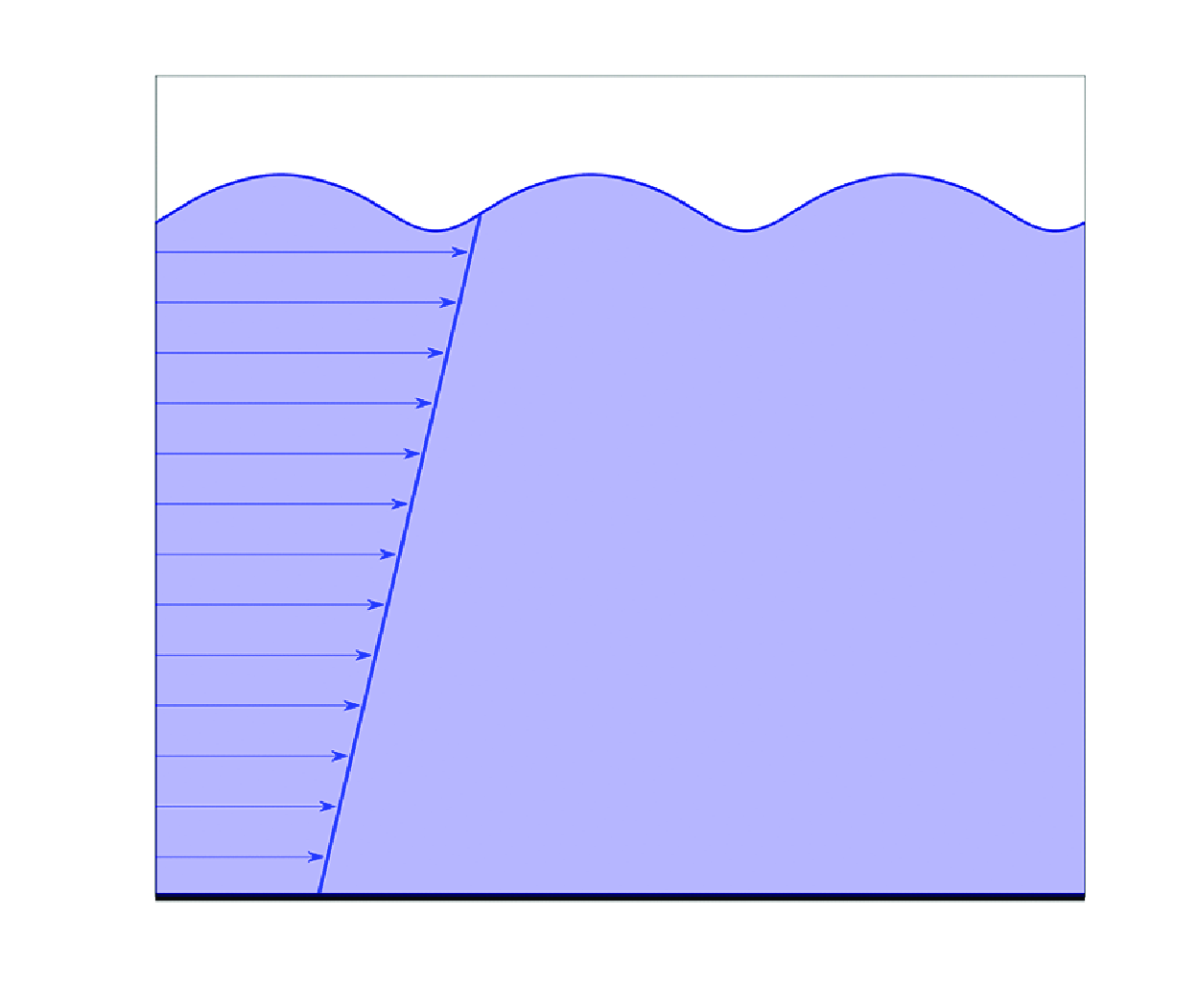
The unperturbed flow is a weakly nonlinear capillary wave train travelling steadily at the free surface of a vertically sheared current of constant vorticity (see figure 1). The fluid is assumed incompressible and inviscid.
In the fixed frame, the underlying current velocity is
 $u_0(y)=U_0+\varOmega y$
, where
 $\varOmega$
is the shear (the current intensity) and
 $U_0$
the current velocity at the free surface
 $y=0$
. The waves are stationary on a stream. Note that the vorticity is
 $-\varOmega$
. Downstream propagation corresponds to negative vorticity, whereas upstream propagation corresponds to positive vorticity.
Being primarily interested in the effect of the vorticity, we choose a reference frame moving with
 $U_0$
(see figure 1). In the moving frame, the fluid velocity is
 \begin{align} {\textbf {u}}(x,y)=(\varOmega y + \phi _x, \phi _y), \end{align}
where
 $(\phi _x,\phi _y)$
is the wave-induced velocity.
Sketches of waves on a shear current in the moving reference frame. Downstream propagation (a). Upstream propagation (b).

The waves are potential due to the Kelvin theorem, which states that vorticity is conserved for a two-dimensional flow of an incompressible and inviscid fluid with external forces derived from a potential. There is no loss of generality if the study is restricted to carrier waves with positive phase speeds, so long as both positive and negative values of
 $\varOmega$
are considered.
The governing equations are the Laplace equation (2.2) with the kinematic and dynamic boundary conditions (2.3)–(2.4) and the bottom condition (2.5):
 \begin{equation} \Delta \phi (x,y,t)=0, \quad -h \lt y \lt \zeta (x,t), \end{equation}
where
 $\zeta (x,t)$
is the surface elevation,
 \begin{align}&\qquad\qquad\qquad \zeta _t+\zeta _x(\phi _x+\varOmega y)-\phi _y=0, \quad y=\zeta (x,t), \end{align}
 \begin{align}& \phi _t+\frac {1}{2}(\nabla \phi )^2+\varOmega \zeta \phi _x -\varOmega \psi -\frac {T}{\rho _w}\frac {\zeta _{xx}}{(1+\zeta _x^2)^{3/2}}=-\frac {P_a}{\rho _w}, \quad y=\zeta (x,t), \end{align}
where
 $\psi$
is the stream function and
 $\rho _w$
the water density. The surface tension
 $T$
is assumed constant.
Without loss of generality, the atmospheric pressure,
 $P_a$
, is set equal to zero:
 \begin{equation} \phi _y=0, \quad y=-h. \end{equation}
Following Thomas, Kharif & Manna (Reference Thomas, Kharif and Manna2012) and Hsu et al. (Reference Hsu, Kharif, Abid and Chen2018), the stream function
 $\psi$
can be removed by differentiating (2.4) with respect to
 $x$
and using the Cauchy–Riemann relations. (Here
 $f(z)=\phi (x,y)+i\psi (x,y)$
with
 $z=x+iy$
where
 $\phi$
is harmonic and
 $\psi =H(\phi )$
its Hilbert transform. Consequently,
 $f$
is holomorphic and satisfies the Cauchy–Riemann relations.) The dynamic boundary condition becomes for weakly nonlinear water waves
 \begin{align} \phi _{tx}&+\phi _{ty}\zeta _x+\phi _x(\phi _{xx}+\phi _{xy}\zeta _x)+\phi _y(\phi _{xy}+\phi _{yy}\zeta _x)+\varOmega \zeta (\phi _{xx}+\phi _{xy}\zeta _x)+\varOmega \phi _y\nonumber \\ &-\frac {T}{\rho _w}\left(\zeta _{xxx}-\frac {3}{2}\zeta _x^2\zeta _{xxx}-3\zeta _{xx}^2\zeta _x\right)=0,\quad y=\zeta (x,t). \end{align}
Equation (2.6) corresponds to that of Hsu et al. (Reference Hsu, Kharif, Abid and Chen2018) for
 $g=0$
.
Hsu et al. (Reference Hsu, Kharif, Abid and Chen2018) used the method of multiple scales to derive the spatio-temporal evolution of the complex envelope,
 $a(\xi ,\tau )$
, of the free surface elevation
 $\zeta (x,t)$
:
 \begin{equation} \zeta (x,t)=\frac {1}{2}\left \lbrace \epsilon a(\xi ,\tau )\exp (i(kx-\omega t))+\text{c.c.} \right \rbrace + \mathcal{O}(\epsilon ^2), \end{equation}
where
 $\xi =\epsilon (x-c_g t)$
,
 $\tau =\epsilon ^2 t$
,
 $c_g$
,
 $k$
and
 $\omega$
are the group velocity, wavenumber and frequency of the carrier wave and
 $\epsilon$
a small parameter.
2.1. Expression of dispersive and nonlinear coefficients
To obtain the dispersive and nonlinear coefficients
 $L$
and
 $N$
of the vor-NLS equation for pure capillary wave trains, we used the expressions we derived for gravity–capillary waves in finite depth and in the presence of vorticity (see equation (2.31) of Hsu et al. (Reference Hsu, Kharif, Abid and Chen2018)) when
 $\kappa$
goes to infinity. The limit of the dispersive coefficient is obtained easily whereas the limit of the nonlinear coefficient needs to be handled carefully because two terms go to infinity. Fortunately, these two infinite terms cancel each other as is shown in the Appendix.
The NLS equation governing the evolution of the complex envelope of a packet of capillary waves on finite depth in the presence of constant vorticity (vor-NLS) is
 \begin{equation} ia_{\tau }+L a_{\xi \xi }+N|a|^2 a=0, \end{equation}
with
 \begin{align} L = \frac {\omega }{k^2(2+X)^3\sigma ^2} & \big[3(1+X)(1+X+X^2)\sigma ^2 -6(1+X)^2\mu \sigma (\sigma ^2-1) \nonumber \\& +\mu ^2(\sigma ^2-1) \big((1+X)^2+(3+2X)\sigma ^2 \big) \big] \end{align}
and
 \begin{align} N&=-\frac {\omega k^2}{8\sigma ^2} \left [\sigma ^2\frac {5+3X}{2+X}-\frac {P_0+P_1X+P_2X^2+P_3X^3+X^4}{(3-\sigma ^2+3X)(2+X)} +2\sigma (2+X) \right. \nonumber \\[5pt]& \quad \left.\left ( \frac {(1+X)^2-\sigma ^2}{\big(1-\sigma ^2\big)\mu +3\sigma (1+X)} +\frac {1-\sigma ^2}{\mu (\big(1-\sigma ^2\big)+X(2+X))+3\sigma (1+X)} \right )\right ], \end{align}
with
 $\mu =kh$
,
 $\sigma =\tanh {\mu }$
,
 $X=\sigma \varOmega /\omega$
and
 $P_0=21-10\sigma ^2+\sigma ^4$
,
 $P_1=42+2\sigma ^2-4\sigma ^4$
,
 $P_2=30+12\sigma ^2$
,
 $P_3=9+5\sigma ^2.$
Note that
 $|X|$
can be considered as a Strouhal number, which is the ratio between the characteristic frequency of the vorticity and that of the capillary waves.
The coefficients
 $L$
and
 $N$
given by (2.9) and (2.10) correspond to those of Hsu et al. (Reference Hsu, Kharif, Abid and Chen2018) for
 $\kappa =k^2 T/(\rho _w g) \rightarrow \infty$
and
 $\varOmega \neq 0$
and to those of Djordjevic & Redekopp (Reference Djordjevic and Redekopp1977) in finite depth for
 $\kappa \rightarrow \infty$
and
 $\varOmega =0$
.
The linear dispersion relation of capillary waves in the presence of constant vorticity is
 \begin{equation} \omega ^2+\sigma \varOmega \omega -\sigma \frac {k^3 T}{\rho _w}=0. \end{equation}
From (2.11) it is easy to show that
 $X\gt -1$
.
As emphasised above, we consider a carrier wave propagating from left to right of frequency
 $\omega$
, phase velocity
 $c_p$
and group velocity
 $c_g$
whose expressions are
 \begin{align}&\qquad\qquad\qquad\qquad\, \omega =-\frac {\sigma \varOmega }{2}+\sqrt {\left(\frac {\sigma \varOmega }{2}\right)^2+\sigma \frac {k^3 T}{\rho _w}},\\[-8pt]\nonumber \end{align}
 \begin{align}&\qquad\qquad\qquad\qquad c_p=-\frac {\sigma \varOmega }{2k}+\sqrt {\left(\frac {\sigma \varOmega }{2k}\right)^2+\sigma \frac {k T}{\rho _w}},\\[-8pt]\nonumber \end{align}
 \begin{align}& c_g=-\frac {\varOmega h}{2}\big(1-\sigma ^2\big)+\frac {\big(1-\sigma ^2\big)(\varOmega ^2h\sigma /2+\mu k^2T/\rho _w)+3\sigma k^2T/\rho _w}{\sqrt {(\varOmega \sigma )^2+4\sigma k^3 T/\rho _w}}. \end{align}
2.2. The Wilton ripple phenomenon and resonant triads
The nonlinear coefficient
 $N$
presents two singularities that one should avoid, either
 \begin{equation} 3-\sigma ^2+3X=0 \end{equation}
or
 \begin{equation} \mu (\big(1-\sigma ^2\big)+X(2+X))+3\sigma (1+X)=0. \end{equation}
Equation (2.15) corresponds to the reduction of the second-harmonic resonance condition of gravity–capillary waves propagating at the free surface of an underlying current of constant vorticity when
 $g$
goes to zero (
 $\kappa$
goes to
 $\infty$
). This resonance which is also called the Wilton ripple phenomenon occurs when both the fundamental mode and the second harmonic have the same phase velocity, that is, when the phase velocity presents a minimum value. Note that in the absence of positive vorticity (
 $\varOmega \lt 0$
) there is no minimum of phase velocity for pure capillary waves. Martin & Matioc (Reference Martin and Matioc2013) proved rigorously the existence of Wilton ripples on finite depth for gravity–capillary water waves with constant positive and negative values of the vorticity. The fact that the phenomenon of Wilton ripples for pure capillary waves occurs only for waves propagating from left to right on a current of positive vorticity is a consequence of their lemma 2.5. Using a different approach to investigate the Wilton ripple phenomenon of pure capillary waves our result agrees with that of Martin & Matioc (Reference Martin and Matioc2013). Note that their study focused on integer values of the wavenumber. The phase velocity
 $c_p$
reaches a minimal value when
 $\varOmega \lt 0$
(positive vorticity) and
 $k=k_m$
given in deep water by
 \begin{equation} k_m=\left (\frac {2\rho _w}{T}\varOmega ^2 \right )^{1/3}. \end{equation}
The wavenumber
 $k$
satisfying
 $c_p(k)=c_p(2k)$
is
 \begin{equation} k=\left (\frac {3\rho _w}{4T} \varOmega ^2 \right )^{1/3}. \end{equation}
The second-harmonic resonance corresponds to the following degenerate resonant triad:
 \begin{align}&\, 2k_1-k_2=0,\\[-10pt]\nonumber \end{align}
 \begin{align}& 2\omega _1-\omega _2=0, \end{align}
where
 \begin{align}& \omega _1=-\frac {\varOmega }{2}+\sqrt {\left(\frac {\varOmega }{2}\right)^2 + \frac {T}{\rho _w} k^3},\\[-6pt]\nonumber \end{align}
 \begin{align}& \omega _2=-\frac {\varOmega }{2}+\sqrt {\left(\frac {\varOmega }{2}\right)^2 + \frac {8T}{\rho _w} k^3}, \end{align}
with
 $k$
given by (2.18).
Injecting the expression of
 $k$
in (2.21) and (2.22), we obtain
 $\omega _1=-3\varOmega /2$
and
 $\omega _2=-3\varOmega$
.
Constantin & Kartashova (Reference Constantin and Kartashova2009) showed that only positive vorticity (
 $\varOmega \lt 0$
) can trigger the occurrence of three-wave resonant interactions of capillary water waves on an underlying current of constant vorticity. As in Martin & Matioc (Reference Martin and Matioc2013) they considered integer values of the wavenumber. Later on, using the methods of Constantin & Kartashova (Reference Constantin and Kartashova2009), Martin (Reference Martin2017) investigated three-wave resonances in deep water to extend their results to gravity–capillary waves. He demonstrated that three-wave resonances of gravity–capillary waves occur only for positive values of the vorticity.
We have shown that the Wilton ripple phenomenon exists in infinite depth for pure capillary waves travelling on a current of constant positive vorticity. To a given fixed value of the vorticity,
 $-\varOmega$
, corresponds a resonant real-valued wavenumber given by (2.18); and conversely, to a given fixed real-valued resonant wavenumber,
 $k$
, corresponds a value of the shear
 $\varOmega =-\sqrt {4Tk^3/(3\rho _w)}$
. Fixing
 $k=1$
gives the minimal value of the vorticity found by Constantin & Kartashova (Reference Constantin and Kartashova2009). Note that within the framework of capillary water waves, the vorticity must be strong to trigger the second-harmonic resonance.
The wavenumber given by (2.18) does not satisfy equation (2.15) unless
 $\sigma =1$
that does not mean that there are no second-harmonic resonances in finite depth within the framework of pure capillary waves.
The second singularity corresponds to the reduction of the short-wave/long-wave resonance of gravity–capillary waves propagating at the free surface of an underlying current of constant vorticity when
 $g$
goes to zero. Note that this singularity disappears in the nonlinear coefficient
 $N$
when
 $\sigma =1$
, that is, in deep water. Nevertheless, this does not mean that there are no resonant triad interactions in deep water.
Equation (2.16) has two real-valued negative roots: one is less than
 $-1$
and is ruled out because
 $X\gt -1$
and the other belongs to
 $(-1,0)$
when
 $\mu$
ranges from zero to infinity. It is useful to note that whatever the depth, there exists a singular value of
 $X$
for
 $-1\lt X\lt 0$
. Constantin & Kartashova (Reference Constantin and Kartashova2009) demonstrated that in deep water, capillary waves on a current of positive vorticity (
 $\varOmega \lt 0$
) may give rise to resonant triads.
We found in finite depth triads of capillary waves satisfying the following resonance conditions:
 \begin{align}&\,\, k_1-k_2+k_3=0, \end{align}
 \begin{align}& \omega _1-\omega _2+\omega _3=0, \end{align}
with
 \begin{equation} \omega _i=-\frac {\sigma \varOmega }{2}+\sqrt {\left(\frac {\sigma \varOmega }{2}\right)^2+\sigma \frac {k_i^3 T}{\rho _w}}, \quad i=1,2,3. \end{equation}
To illustrate this feature of capillary waves on a current of constant positive vorticity in finite depth, three examples are shown in figure 2 which gives pairs of capillary waves of wavenumbers
 $(k_1,k_2)$
that excite a third wave of wavenumber
 $k_3$
. To a given value of
 $k_1$
corresponds a value of
 $k_2$
and consequently a value of
 $k_3$
. The three curves present a minimum for the wavenumber
 $k_2$
.
We can conclude that (2.16) corresponds to resonant triads of capillary waves in finite depth with positive constant vorticity. At any depth, there exists a forbidden positive vorticity value corresponding to a resonant triad.
Resonant triad in finite depth: a pair of wavenumbers
 $(k_1, k_2)$
exciting a third wavenumber
 $k_3=k_2-k_1$
. Here
 $\mu =1$
(black solid line),
 $\mu =0.5$
(red solid line),
 $\mu =0.3$
(blue solid line), with
 $\varOmega =-1 \,{\textrm s}^{-1}$
and wavenumbers in
 ${\textrm m}^{-1}$
.

3. Stability of weakly nonlinear capillary waves on arbitrary depth with constant vorticity
The three-wave interactions are most frequently considered the most likely dominant wave–wave interaction among pure capillary waves. However, Shats, Punzmann & Xia (Reference Shats, Punzmann and Xia2010) showed experimentally that the nonlinear four-wave interaction due to modulational instability can be dominant. To shed light on the physical processes governing the formation of steep wave events they considered parametrically excited capillary waves. The new and unexpected finding of their experiments on pure capillary waves was that the dominant wave interaction in the formation of rogue waves is due to modulational instability which is an inseparable feature of the NLS equation that has been used intensively to explain the occurrence of rogue waves. These experiments show the relevance of the study of modulational instability of capillary water waves. Furthermore, the impact of a two-dimensional underlying shear current on these wave–wave interactions is an important issue.
Using a Hamiltonian approach, Zakharov (Reference Zakharov1968) derived in the context of gravity waves on deep water the famous NLS equation and showed that Stokes wave trains are unstable to modulational long-wave perturbations. For a detailed history on the modulational instability the reader may refer to the review paper of Zakharov & Ostrovsky (Reference Zakharov and Ostrovsky2009).
The NLS equation (2.8) admits the Stokes wave solution
 \begin{equation} a=a_0\exp \big(iNa_0^2 \tau \big), \end{equation}
where
 $a$
is the complex amplitude of the Stokes wave with
 $a_0$
real which is the modulus of the complex envelope.
Let us consider an infinitesimal disturbance of this solution so that the perturbed solution is written as follows:
 \begin{equation} a^{\prime}=a_0 \big(1+\delta _a\big) \exp \big(iNa_0^2 \tau \big) \exp (i\delta _w). \end{equation}
Substituting the expression (3.2) of the perturbed solution in the NLS equation (2.8), linearising and separating between real and imaginary parts leads to a system of linear coupled partial differential equations with constant coefficients. Consequently, this system admits solutions of the following forms:
 \begin{align} \delta _a&=(\delta _a)_0 \exp \left(i\left(p\xi -\Gamma \tau \right)\right), \end{align}
 \begin{align} \delta _w&=(\delta _w)_0 \exp \left(i\left(p\xi -\Gamma \tau \right)\right), \end{align}
where the real
 $p$
is the perturbation wavenumber.
The necessary and sufficient condition for the existence of a non-trivial solution is
 \begin{equation} \varGamma ^2=p^2\big(L^2p^2-2NLa_0^2\big). \end{equation}
The Stokes wave solution is stable when
 $L^2p^2-2NLa_0^2 \geqslant 0$
and unstable when
 $L^2p^2-2NLa_0^2 \lt 0$
.
The growth rate of instability is
 \begin{equation} \varGamma _i=p\big(2NLa_0^2-L^2p^2\big)^{1/2}. \end{equation}
The maximal growth rate of instability is
 \begin{equation} \varGamma _{imax}=\sqrt {\frac {N}{L}}\sqrt {NL} a_0^2, \end{equation}
for
 $p=\sqrt {({N}/{L})} a_0$
.
Note that instability occurs when
 $LN\gt 0$
.
For
 $\varOmega =0$
the rate of growth of the modulational instability of pure capillary waves on finite depth is
 \begin{equation} \varGamma _i=\frac {\omega }{8k^2}\sqrt {3a_0^2k^4p^2-9p^4}, \end{equation}
which can be found in Chen & Saffman (Reference Chen and Saffman1985) and Hsu et al. (Reference Hsu, Kharif, Abid and Chen2018). The maximum growth rate is
 $\omega (a_0k)^2/16$
, corresponding to the wavenumber
 $p_{{max}}=a_0k^2/\sqrt {6}$
.
We introduce dimensionless coefficients
 $\tilde {L}=k^2 L/\omega$
and
 $\tilde {N}=N/(\omega k^2)$
so that the dispersive and nonlinear coefficients of the NLS equation are functions of
 $\mu =kh$
and
 $X=\sigma \varOmega /\omega$
.
The dimensionless growth rate of instability reads
 \begin{equation} \frac {\varGamma _i}{\omega (a_0 k)^2}=\tilde {p}\big(2\tilde {N}\tilde {L}-\tilde {L}^2\tilde {p}^2\big)^{1/2}, \end{equation}
with
 $\tilde {p}=p/(a_0 k^2)$
and its maximal value is
 \begin{equation} \frac {\varGamma _{imax}}{\omega (a_0 k)^2}=\sqrt {\frac {\tilde {N}}{\tilde {L}}}\sqrt {\tilde {N}\tilde {L}}, \end{equation}
for
 $\tilde {p} = \sqrt {\tilde {N}/\tilde {L}}$
.
Dimensionless growth rate of instability as a function of the dimensionless perturbation wavenumber for
 $kh=0.30$
and
 $X=-0.40$
(orange solid line),
 $X=0$
(blue solid line),
 $X=0.40$
(green solid line).

The dimensionless bandwidth of instability is
 \begin{equation} \Delta \tilde {p}=\sqrt {2\frac {\tilde {N}}{\tilde {L}}}, \quad \frac {\Delta p}{k}=\Delta \tilde {p} \, a_0k. \end{equation}
The analytic expression of the dimensionless maximal growth rate of instability in deep water reads
 \begin{equation} \frac {\varGamma _{imax}}{\omega (a_0 k)^2}=\frac {3+14X+23X^2+11X^3-3X^4}{24(X+1)(3X+2)}. \end{equation}
For weak vorticity, (3.12) becomes
 \begin{equation} \frac {\varGamma _{imax}}{\omega (a_0 k)^2}=\frac {1}{16}\left(1+\frac {13}{6}X+\frac {3}{4}X^2\right)+\mathcal{O}(X^3). \end{equation}
In figures 3
and 4 is plotted the dimensionless growth rate of instability given by (3.9) as a function of the dimensionless perturbation wavenumber
 $\tilde {p}$
for several values of the depth and vorticity. The dimensionless growth rate of instability increases as the dimensionless shear increases and as the dimensionless vorticity decreases for a given value of the depth. This feature can be observed whatever the depth. For negative dimensionless vorticity, the dimensionless growth rate of instability increases as the depth decreases. This feature is still present in shallow water for positive vorticity. The bandwidth of instability increases as the depth decreases.
Figure 5 shows the dimensionless maximal growth rate of instability as a function of the dimensionless depth,
 $\mu =kh$
, for several values of the dimensionless vorticity. We observe that it starts to increase significantly while
 $\mu \lt 2$
. In finite and infinite depths, positive (negative) dimensionless vorticity increases (reduces) the dimensionless growth rate of instability. In shallow water, this feature persists only for weak dimensionless vorticity.
Dimensionless growth rate of instability as a function of the dimensionless perturbation wavenumber for
 $kh=1$
and
 $X=-0.40$
(orange solid line),
 $X=0$
(blue solid line),
 $X=0.40$
(green solid line).

In figure 6 is plotted the dimensionless maximal growth rate of instability as a function of the vorticity for several values of the dimensionless depth. For about
 $X \lt 3$
the dimensionless maximal growth rate of instability increases as the depth decreases, whereas for about
 $X \gt 3$
it increases as the depth increases.
Dimensionless maximal growth rate of instability as a function of the dimensionless depth,
 $\mu =kh$
: (a)
 $X=-0.10$
(orange solid line),
 $X=0$
(blue solid line),
 $X=0.10$
(green solid line); (b)
 $X=1$
(orange solid line),
 $X=1.5$
(blue solid line),
 $X=2$
(green solid line).

Dimensionless maximal growth rate of instability as a function of the vorticity for several dimensionless depths:
 $kh=0.3$
(blue solid line),
 $kh=0.5$
(orange solid line),
 $kh=1$
(green solid line),
 $kh=\infty$
(red solid line). Here
 $\varGamma _{imax0\infty }=\varGamma _{imax}(\varOmega =0,kh=\infty)$
.

Within the framework of irrotational flow (
 $X=0$
), Tiron & Choi (Reference Tiron and Choi2012) investigated the stability of the exact deep-water capillary wave solution, derived by Crapper (Reference Crapper1957), to two-dimensional infinitesimal disturbances. In figure 7 is plotted the dimensionless growth rate as a function of the dimensionless wavenumber of the modulational perturbation for several values of the wave steepness of the carrier wave. The symbols correspond to the results of Tiron & Choi (Reference Tiron and Choi2012) whereas the solid line corresponds to the results obtained with the vor-NLS equation. A quite good agreement between the two approaches is obtained when
 $a_0k \leqslant 0.69$
. Note that the maximal wave steepness of Crapper’s capillary waves is
 $a_0k \approx 2.29$
.
Dimensionless growth rate as a function of the dimensionless perturbation wavenumber in deep water with
 $X=0$
. Circles,
 $a_0k=0.25$
; asterisks,
 $a_0k=0.47$
; diamonds,
 $a_0k=0.69$
; squares,
 $a_0k=1.03$
; stars,
 $a_0k=1.16$
. The symbols correspond to the results of Tiron & Choi (Reference Tiron and Choi2012) and the solid line corresponds to those of the vor-NLS equation.

3.1. Effect of viscosity and forcing
The rate of decay of the amplitude of linear waves due to bulk viscosity is
 $2\nu k^2$
, where
 $\nu$
is the kinematic viscosity and
 $k$
the wavenumber. In the following we consider the modulational instability of capillary waves in the presence of dissipation due to viscosity and some forcing due for instance to wind. Note that this problem has been investigated by Kharif et al. (Reference Kharif, Kraenkel, Manna and Thomas2010) for pure gravity waves in deep water. The latter authors used the Miles mechanism to model wind effect.
Equation (2.8) becomes
 \begin{equation} ia_{\tau }+La_{\xi \xi }+N|a|^2 a=i(\varDelta -2\nu k^2)a, \end{equation}
where
 $\varDelta \gt 0$
corresponds to a forcing term.
When
 $\varDelta =0$
, (3.14) is similar to the NLS equation derived rigorously by Dias, Dyachenko & Zakharov (Reference Dias, Dyachenko and Zakharov2008) within the framework of weakly damped water waves (see their equation (40)).
Equation (3.14) admits the following solution:
 \begin{equation} a_s=a_0\exp ({K\!\tau} ) \exp \left (\frac {iN}{2K}a_0^2\big(e^{2K\!\tau }-1\big) \right ), \end{equation}
where
 $K=\varDelta -2\nu k^2$
.
Note that
 $a_s$
is spatially constant.
We superimpose to this solution a small disturbance:
 \begin{equation} a(\xi ,\tau )=a_s(1+\epsilon a^{\prime}(\xi , \tau )), \end{equation}
with
 $\epsilon \ll 1$
.
Substituting (3.16) into (3.14) and keeping only terms of order
 $\epsilon$
and separating the real and imaginary parts of
 $a^{\prime}(\xi ,\tau )=a^{\prime}_r(\xi ,\tau )+ia^{\prime}_i(\xi ,\tau )$
gives
 \begin{align}& a^{\prime}_{i\tau }-La^{\prime}_{r\xi \xi }-2N a_0^2 \exp (2K\!\tau ) a^{\prime}_r=0, \end{align}
 \begin{align}&\qquad\qquad\quad a^{\prime}_{r\tau }+La^{\prime}_{i\xi \xi }=0. \end{align}
Set
 $a^{\prime}_r(\xi ,\tau )=\mathrm{Re}(a^{\prime}_{r0}(\tau )\exp ( ip\xi ))$
and
 $a^{\prime}_i(\xi ,\tau )=\mathrm{Im}(a^{\prime}_{i0}(\tau )\exp (ip\xi ))$
, where
 $p$
is the wavenumber of the perturbation. Then,
 \begin{align}& \frac {{\textrm d}a^{\prime}_{i0}}{{\textrm d}\tau }+\big(Lp^2-2N a_0^2 \exp (2K\!\tau )\big)a^{\prime}_{r0}=0, \end{align}
 \begin{align}&\qquad\qquad\quad \frac {{\textrm d}a^{\prime}_{r0}}{{\textrm d}\tau }-Lp^2a^{\prime}_{i0}=0. \end{align}
Combining the two previous equations gives
 \begin{equation} \frac {{d}^2a^{\prime}_{r0}}{{\textrm d}\tau ^2}+L^2p^4\left (1-\frac {2N}{Lp^2} a_0^2 \exp (2K\!\tau ) \right )a^{\prime}_{r0}=0. \end{equation}
One may distinguish two cases according to whether
 $K$
is negative or positive.
-
(i) Let
 $K$
be negative. This case was analysed by Segur, Henderson & Carter (Reference Segur, Henderson and Carter2005) and Kharif et al. (Reference Kharif, Kraenkel, Manna and Thomas2010). In the presence of damping, the modulational instability is stabilised by viscous dissipation. However, note that the modulational instability may grow, but its growth is limited and starts to stabilise after a time
$\tau =- ({1}/{2K})\ln ({2Na_0^2}/{Lp^2})$
corresponding to the change of sign of the coefficient of
$a^{\prime}_{r0}$
of (3.21). Note that the bandwidth of instability shrinks as the amplitude of the carrier wave diminishes, resulting in stabilisation of unstable modes. The most unstable perturbation starts stabilisation at
$\tau =\ln 2/(4\nu k^2)$
. Let us consider a carrier wave of wavelength
$\lambda =0.005 \, {\textrm m}$
in deep water. For
$X=0$
, stabilising of the most unstable perturbation will start at
$\tau \approx 7 \tau _0$
, where
$\tau _0$
is the dimensional period of the carrier wave. For
$X=0.4$
and
$X=-0.4$
, we found that the most unstable perturbation stabilises at
$\tau \approx 6 \tau _0$
and
$\tau \approx 9 \tau _0$
, respectively. These critical times are more or less confirmed by numerical simulations of dimensionless equation (3.24) (see figure 8) without forcing.
-
(ii) Let
$K$
be positive. This case was discussed by Kharif et al. (Reference Kharif, Kraenkel, Manna and Thomas2010) who considered gravity wave trains on the surface of water acted upon by wind and under the influence of viscosity. Herein, a similar situation is considered within the framework of pure capillary wave trains. In this case, the modulational perturbations are initially oscillating for
$0 \lt \tau \lt ({1}/{2K})\ln ( {2Na_0^2}/{Lp^2})$
and then start to grow exponentially for
$\tau \gt ({1}/{2K})\ln ( {2Na_0^2}/{Lp^2})$
. The bandwidth of instability increases as the amplitude of the carrier wave increases. Consequently, stable modes may become unstable. Let
$p$
be a perturbation wavenumber corresponding to a stable state. There is a critical value of the carrier wave amplitude,
$a_0$
, for which the bandwidth instability is equal to
$p$
. For carrier wave amplitude larger than this critical value, the perturbation becomes unstable. The critical value is given by
$\varGamma _i=0$
, that is to say,(3.22)The modulational instability will start to grow as soon as the carrier wave amplitude reaches the critical value. When the carrier wave amplitude is set equal to
\begin{equation} a_{0c}^2=\frac {Lp^2}{2N}. \end{equation}
$a_{0c}$
, the instability starts at
$\tau =0$
.


Let us consider the case without vorticity (
 $X=0$
) in deep water. The dispersive and nonlinear coefficients of the vor-NLS equation are
 $L=3\omega /(8k^2)$
and
 $\omega k^2/16$
. The critical wave steepness of the carrier wave is
 \begin{align} a_{0c}k=\sqrt {3}\,p/k .\end{align}
This critical value is more or less confirmed by numerical simulations of dimensionless equation (3.24) (see figure 9
a) with forcing,
 $\tilde {K}=(\tilde {\varDelta }-2/R_e)$
.
For
 $(X,p/k)=(0.4, 0.72)$
and
 $(X,p/k)=(-0.4, 0.59)$
we found, in deep water,
 $a_{0c}k \approx 1$
and
 $1.5$
, respectively (see figure 9
b,c).
To complete the linear stability analysis, we consider the nonlinear evolution of unstable and stable modes. To do this, we use (3.14) written in dimensionless form with respect to the reference length
 $1/k$
and reference time
 $1/\omega$
, where
 $k$
and
 $\omega$
are the wavenumber and frequency of the carrier wave, respectively:
 \begin{equation} i\tilde {a}_{\tilde {\tau }}+\tilde {L}\tilde {a}_{\tilde {\xi } \tilde {\xi }}+\tilde {N}|\tilde {a}|^2 \tilde {a}=i\left(\tilde {\varDelta }-\frac {2}{R_e}\right)\tilde {a}, \end{equation}
where
 $R_e=\omega /(k^2 \nu )$
.
Within the framework of numerical simulations of the vor-NLS equation, figure 8 shows, in the presence of viscous dissipation only and for several values of the vorticity, the temporal evolution of the amplitude of the carrier wave,
 $a_0$
, and those of the most unstable sidebands,
 $a_{-1}$
and
 $a_{+1}$
, whose curves overlap. At the beginning of the nonlinear interaction, the modulational instability is growing due to a transfer of energy from the carrier wave to the sidebands and then stabilises under the effect of the dissipation (see figure 8
a,b). The case corresponding to figure 8(c) presents a different behaviour because the initial rate of growth of the instability and the rate of damping are of the same order, preventing the instability from developing.
Figure 9 shows, in the presence of forcing assumed to be a constant, the temporal evolution of the amplitude of the carrier wave,
 $a_0$
, and those of the initially stable sidebands,
 $a_{-1}$
and
 $a_{+1}$
, for several values of the vorticity. At the beginning, numerical simulations show that the perturbations are oscillating and then are growing.
Temporal evolution of the dimensionless amplitudes of the carrier wave (solid blue line) and most unstable sideband modes (solid red line) in the presence of viscous dissipation in deep water: (a)
 $X=0$
,
 $R_e \approx 240$
; (b)
 $X=0.4$
,
 $R_e \approx 202$
; (c)
 $X=-0.4$
,
 $R_e \approx 308$
. Herein,
 $\omega =1$
.

Temporal evolution of the dimensionless amplitudes of the carrier wave (solid blue line) and stable sideband modes (solid red line) in the presence of weak forcing in deep water: (a)
 $X=0$
,
 $p/k=0.7$
; (b)
 $X=0.4$
,
 $p/k=0.72$
; (c)
 $X=-0.4$
,
 $p/k=0.59$
;
 $\tilde {K}=3/10\,000$
. Herein,
 $\omega =1$
.

4. Capillary solitary waves on deep water in the presence of constant vorticity
Equation (2.8) admits as solution the envelope soliton given by the following expression:
 \begin{equation} a(\xi ,\tau )=\pm a_0 \textrm{sech} \left (a_0\left(\frac {N}{2L}\right)^{1/2} \xi \right ) \exp (iNa_0^2 \tau /2). \end{equation}
The corresponding surface elevation of a weakly nonlinear wave train of envelope given by (4.1) is
 \begin{equation} \zeta =\pm \frac {1}{2}\epsilon a_0 \,\textrm{sech} \left (\sqrt {\frac {N}{2L}}\, a_0\epsilon (x-c_g t)\right ) \exp \left (ikx-i\left(\omega -\frac {N}{2}\epsilon ^2a_0^2\right)t\right ) + \text{c.c.}, \end{equation}
where
 $k$
and
 $\omega$
are the carrier wavenumber and carrier frequency and
 $\text{c.c.}$
is the complex conjugation.
Near the minimum of phase velocity of linear gravity–capillary waves, the phase velocity and the group velocity are nearly equal. As stated by Longuet-Higgins (Reference Longuet-Higgins1993) in any dispersive medium supporting an envelope soliton and whose linear dispersion has an extremum we can expect that steady solitary waves with decaying oscillatory tails bifurcate from linear periodic waves. These waves are called generalised solitary waves to distinguish them from those which are flat at
 $x=\pm \infty$
. For a review on this problem, the reader is referred to Dias & Kharif (Reference Dias and Kharif1999). It is noteworthy to emphasise that a pure periodic capillary wave train can bifurcate into generalised solitary waves only in the presence of positive vorticity as mentioned in § 2. Bifurcation cannot occur for negative vorticity because there is no phase velocity minimum.
Following Akylas (Reference Akylas1993) and Abid et al. (Reference Abid, Kharif, Hsu and Chen2019) we consider a train of periodic pure capillary waves on deep water bifurcating into a solitary wave with a decaying oscillatory tail in the presence of positive vorticity (
 $\varOmega \lt 0$
). Note that Akylas (Reference Akylas1993) and Abid et al. (Reference Abid, Kharif, Hsu and Chen2019) considered gravity–capillary waves.
We use
 $T/(\rho _w c^2)$
and
 $T/(\rho _w c^3)$
as unit of length and unit of time, where
 $c$
is the phase velocity of the envelope soliton. In this way
 $c$
is the reference phase velocity scale. Note that this normalisation is equivalent to setting
 $T=1$
,
 $\rho _w=1$
and
 $c=1$
.
Within the framework of the new normalisation, the condition for the envelope soliton to be a solitary is
 \begin{equation} \omega (k,\varOmega )-\frac {1}{2}Na_0^2\epsilon ^2=k, \quad \frac {\partial \omega }{\partial k}=1. \end{equation}
Critical values of the parameters are obtained by setting
 $\epsilon =0$
in (4.3):
 \begin{equation} k_0=\omega (k_0,\varOmega _0), \quad \frac {\partial \omega }{\partial k}(k_0,\varOmega _0)=1. \end{equation}
Solving these two equations gives
 \begin{equation} k_0=\frac {1}{2}, \quad \varOmega _0=-\frac {1}{4}, \quad \omega _0=\frac {1}{2}. \end{equation}
The carrier wavenumber
 $k$
and the shear
 $\varOmega$
are expanded about (
 $k_0, \varOmega _0$
) as follows:
 \begin{align}&\,\,\, k=k_0+k_1 \epsilon ^2 + \mathcal{O}(\epsilon ^3), \end{align}
 \begin{align}& \varOmega =\varOmega _0+\varOmega _1 \epsilon ^2 + \mathcal{O}(\epsilon ^3). \end{align}
Expanding
 $\omega (k,\varOmega )$
about (
 $k_0, \varOmega _0$
) and using
 \begin{align} k=\omega (k,\varOmega )-\frac {1}{2}N\epsilon ^2 a_0^2, \end{align}
with
 $\partial \omega /\partial k(k_0,\varOmega _0)=1$
, gives
 \begin{align}&\,\, \varOmega _1=\frac {1}{2}\frac {N(k_0,\varOmega _0)}{\dfrac {\partial \omega }{\partial \varOmega }(k_0,\varOmega _0)} a_0^2,\\[-10pt]\nonumber \end{align}
 \begin{align}& k_1=-\frac {\dfrac {\partial ^2\omega }{\partial k \partial \varOmega }(k_0,\varOmega _0)}{2L(k_0,\varOmega _0)} \varOmega _1. \end{align}
Let
 $\delta \varOmega$
be the difference between
 $\varOmega$
and the critical value
 $\varOmega _0$
:
 \begin{align} \delta \varOmega =\varOmega _1 \epsilon ^2 + \mathcal{O}(\epsilon ^3). \end{align}
The square of the amplitude of the generalised solitary wave is
 \begin{equation} a_0^2 \epsilon ^2=2\frac {\dfrac {\partial \omega }{\partial \varOmega }(k_0,\varOmega _0)}{N(k_0,\varOmega _0)} \delta \varOmega \end{equation}
and
 \begin{equation} k=k_0-\frac {\dfrac {\partial ^2 \omega }{\partial k \partial \varOmega }(k_0,\varOmega _0)}{2L(k_0,\varOmega _0)} \delta \varOmega. \end{equation}
Substituting the critical values given by (4.5) into (4.12) and (4.13) gives
 \begin{align}& a_0^2\epsilon ^2=-\frac {32^2}{3} \delta \varOmega , \quad \delta \varOmega \lt 0, \end{align}
 \begin{align}&\,\, k=k_0-\frac {3}{16} \delta \varOmega , \quad \delta \varOmega \lt 0. \end{align}
Consequently, the profile of the generalised solitary wave is
 \begin{equation} \zeta (x,t)=\pm \frac {32}{\sqrt {3}} \sqrt {-\delta \varOmega }\, \textrm{sech}\left (\sqrt {-\delta \varOmega } (x-t) \right ) \cos \left (k(x-t)\right ). \end{equation}
The profile of the generalised solitary wave is known once the bifurcation parameter
 $\delta \varOmega$
is fixed. At
 $\varOmega =\varOmega _0$
the train of linear periodic capillary waves bifurcates into a solitary wave whose profile is given by (4.16). The
 $(+)$
sign corresponds to a generalised solitary wave of elevation, whereas the
 $(-)$
sign corresponds to a generalised solitary wave of depression.
The envelope soliton is unstable to transverse perturbations (see § 5). Consequently, capillary solitary waves with decaying oscillatory tails are expected to be unstable, too.
Within the framework of irrotational flow, Ifrim & Tataru (Reference Ifrim and Tataru2020) proved rigorously that there are no capillary solitary waves in deep water with a free surface asymptotically flat at infinity. We have shown that capillary solitary waves with decaying oscillatory tails in the presence of constant positive vorticity may exist in deep water. Within the framework of rotational flows, we have shown that generalised capillary solitary waves may exist. In figures 10 and 11 are plotted the dimensionless profiles of generalised capillary solitary waves in deep water for two values of the bifurcation parameter
 $\delta \varOmega$
. The profiles become flatter when
 $|\delta \varOmega |$
increases. This feature could suggest the existence of capillary solitary waves being flat in the far field at the free surface of rotational flows of positive vorticity in deep water.
Dimensionless profiles of generalised capillary solitary waves of elevation (a) and depression (b) in deep water for
 $\delta \varOmega =-0.01$
.

Dimensionless profiles of generalised capillary solitary waves of elevation (a) and depression (b) in deep water for
 $\delta \varOmega =-0.05$
.

5. Transverse instability of the capillary envelope soliton and capillary Stokes wave in deep water with constant vorticity
Within the framework of deep water, Ellingsen (Reference Ellingsen2016) showed that a wave of weak amplitude can propagate at an angle on a vertically sheared current without introducing additional vorticity, if the vorticity is also weak. He also emphasised that this claim can be applied to linear waves propagating in finite depth (Ellingsen Reference Ellingsen2014). Consequently, results presented in the following two subsections concern capillary waves travelling on a shear current of weak vorticity.
In the two following subsections, we consider the stability of the capillary envelope soliton and capillary Stokes waves to transverse perturbations. Note that the vorticity of the underlying current is now perturbed by the infinitesimal periodic vorticity due to the perturbation, while in one-dimensional propagation the perturbation is potential and does not affect the shear. Nevertheless, the phase average of the vorticity is
 $-\varOmega$
.
5.1. Capillary envelope soliton
In two dimensions the NLS equation in deep water reads
 \begin{equation} ia_{\tau }+L a_{\xi \xi }+M a_{\eta \eta }+N|a|^2 a=0, \end{equation}
with
 \begin{align}&\qquad L=\frac {3\omega }{k^2} \left (\frac {(1+X)(1+X+X^2)}{(2+X)^3} \right ),\\[-10pt]\nonumber \end{align}
 \begin{align}& N=\frac {\omega k^2}{24} \left (\frac {3+14X+23X^2+11X^3-3X^4}{(X+1)(3X+2)} \right ),\\[-10pt]\nonumber \end{align}
 \begin{align}&\qquad\qquad M=\frac {3T}{2\rho _w} \left (\frac {k}{\omega (2+X)} \right ). \end{align}
Here in
 $X=\varOmega /\omega$
.
Equation (5.1) admits as solution the two-dimensional envelope soliton,
 $\bar {a}(\xi ,\tau )$
, given by (4.1). We consider the stability of this solution to infinitesimal disturbances:
 \begin{equation} a(\xi ,\eta , \tau )=\bar {a}(\xi ,\tau )+a^{\prime}(\xi ,\eta ,\tau )\exp \big(iNa_0^2\tau /2\big). \end{equation}
The stability analysis is similar to that used by Abid et al. (Reference Abid, Kharif, Hsu and Chen2019) for gravity–capillary envelope soliton, except that now the coefficients of the NLS equation correspond to pure capillary envelope soliton. Linearisation of (5.1) about
 $\bar {a}$
with
 $a^{\prime}=u+iv$
gives
 \begin{align}& v_{\tau }=Lu_{\xi \xi }+Mu_{\eta \eta }+\Big(3NA^2-Na_0^2/2\Big)u,\\[-10pt]\nonumber \end{align}
 \begin{align}& u_{\tau }=-Lv_{\xi \xi }-Mv_{\eta \eta }-\Big(NA^2-Na_0^2/2\Big)v, \end{align}
where
 \begin{align} A=a_0\textrm{sech} \left (a_0\left(\frac {N}{2L}\right)^{1/2} \xi \right ). \end{align}
The system (5.6)–(5.7) of linear partial differential equations with constant coefficients admits solutions of the following form:
 \begin{align}& u=\hat {u}(\xi )\exp (\textit{iq}\eta +\Gamma \tau ),\\[-10pt]\nonumber \end{align}
 \begin{align}& v=\hat {v}(\xi )\exp (\textit{iq}\eta +\Gamma \tau ). \end{align}
Substitution of (5.9) and (5.10) into (5.6) and (5.7) gives
 \begin{align}& \varGamma \hat {v}=L\frac {{d}^2\hat {u}}{{\textrm d}\xi ^2} -Mq^2 \hat {u} +\Big(3NA^2-Na_0^2/2\Big)\hat {u},\\[-10pt]\nonumber \end{align}
 \begin{align}& \varGamma \hat {u}=-L\frac {{d}^2\hat {v}}{{\textrm d}\xi ^2} +Mq^2 \hat {v} -\Big(NA^2-Na_0^2/2\Big)\hat {v}. \end{align}
The eigenfunction
 $\hat {v}$
can be eliminated:
 \begin{equation} \varGamma ^2 \hat {u}=-\big(D_0-Mq^2\big)\big(D_1-Mq^2\big)\hat {u}, \end{equation}
with
 \begin{align} D_0&=L\frac {{d}^2}{{\textrm d}\xi ^2}+NA^2-Na_0^2/2,\\[-10pt]\nonumber \end{align}
 \begin{align} D_1&=L\frac {{d}^2}{{\textrm d}\xi ^2}+3NA^2-Na_0^2/2. \end{align}
The eigenfunction
 $\hat {u} \rightarrow 0$
as
 $\xi \rightarrow \infty$
(the eigenfunctions are local in
 $\xi$
). Note that the non-local states corresponding to the continuum spectrum are stable or marginally stable (Saffman & Yuen Reference Saffman and Yuen1978; Rypdal & Rasmussen Reference Rypdal and Rasmussen1989). Zakharov & Rubenchik (Reference Zakharov and Rubenchik1974) investigated analytically the transverse instability of envelope solitons.
The numerical method used to solve (5.13) is outlined in Appendix A of Abid et al. (Reference Abid, Kharif, Hsu and Chen2019).
Without loss of generality, we set
 $T=1$
,
 $\rho _w=1$
and
 $k=1$
as in Saffman & Yuen (Reference Saffman and Yuen1985) and Tiron & Choi (Reference Tiron and Choi2012). For the sake of clarity, the same symbols are used for the coefficients of the NLS equation. For comparison, we consider the analytic expression of the instability growth rate derived by Rypdal & Rasmussen (Reference Rypdal and Rasmussen1989) and Abid et al. (Reference Abid, Kharif, Hsu and Chen2019), given in dimensionless form by
 \begin{align}& \varGamma ^2=\frac {32}{\pi ^2}MN q^2\left(1-\frac {M}{3N} q^2\right),\\[-10pt]\nonumber \end{align}
 \begin{align}&\qquad\quad \varGamma _{max}^2=\frac {24}{\pi ^2}N^2, \end{align}
with
 \begin{align} q_{max}=\sqrt {\frac {3N}{2M}.} \end{align}
The capillary envelope soliton is unstable to infinitesimal transverse perturbations of wavenumber
 $q$
satisfying
 $q^2 \lt 3N/M$
. Figure 12 shows the square of the dimensionless growth rate as a function of the square of the dimensionless transverse wavenumber for different values of the vorticity. The numerical and analytical results are in excellent agreement. The dimensionless growth rate and instability bandwidth increase as the dimensionless vorticity decreases. Note that in deep water
 \begin{align} \varOmega ^2=\frac {Tk^3}{\rho _w} \frac {X^2}{1+X} \quad \textrm{with} \ X\gt -1, \end{align}
and in dimensionless form
 \begin{align} \varOmega ^2=\frac {X^2}{1+X}. \end{align}
Square of the dimensionless growth rate of the transverse unstable mode of capillary envelope soliton in deep water as a function of the square of the dimensionless wavenumber for
 $X=-0.1$
(stars),
 $X=0$
(solid line),
 $X=0.1$
(circles). The dashed lines correspond to the analytical expression given by (5.16).

5.2. Capillary Stokes waves
Equation (5.1) admits as solution the Stokes wave envelope given by (3.1). This solution is unstable to perturbations of longitudinal and transverse wavenumbers
 $p$
and
 $q$
if
 \begin{equation} Lp^2+Mq^2\lt 2Na_0^2. \end{equation}
Using the linear dispersion (2.11) the coefficient
 $M$
is rewritten as follows:
 \begin{equation} M=\frac {3\omega }{2k^2}\frac {1+X}{2+X}. \end{equation}
In a more explicit form, condition (5.21) reads
 \begin{equation} \frac {3(1+X)(1+X+X^2)}{(2+X)^3}\,p^2+\frac {3(1+X)}{2(2+X)}\,q^2\lt \frac {3+14X+23X^2+11X^3-3X^4}{12(1+X)(2+3X)}\,a_0^2k^4. \end{equation}
The instability condition
 $p^2+2q^2\lt k^4 a_0^2/3$
, established by Chen & Saffman (Reference Chen and Saffman1985), is recovered for
 $X=0$
.
The square of growth rate of instability is
 \begin{equation} \varGamma _i^2=\big(Lp^2+Mq^2\big)\big(2Na_0^2-Lp^2-Mq^2\big). \end{equation}
Substituting the expressions of
 $L$
,
 $M$
and
 $N$
into (5.24), we obtain in dimensionless form
 \begin{align} \frac {\varGamma _i^2}{\omega ^2}&=\frac {3(1+X)}{2+X}\left (\frac {1+X+X^2}{(2+X)^2}\frac {p^2}{k^2}+\frac {q^2}{2k^2}\right )\nonumber \\ & \quad \times \left (\frac {3+14X+23X^2+11X^3-3X^4}{12(1+X)(2+X)}a_0^2k^2 - \frac {3(1+X)}{2+X}\left (\frac {1+X+X^2}{(2+X)^2}\frac {p^2}{k^2}+\frac {q^2}{2k^2}\right )\right ). \end{align}
For
 $X=0$
we recover the growth rate of instability of Chen & Saffman (Reference Chen and Saffman1985) given by
 \begin{equation} \varGamma _i=\frac {1}{8}\left(3a_0^2k^3\big(p^2+2q^2\big)-\frac {9}{k}\big(p^2+2q^2\big)^2 \right)^{1/2}. \end{equation}
Note that Chen & Saffman (Reference Chen and Saffman1985) used the relation
 $\omega ^2=k^3$
.
Infinite-depth stability diagram in the
 $(p/k,q/k)$
plane for
 $a_0k=0.1$
and three values of the vorticity. Blue:
 $X=0$
; orange:
 $X=-0.1$
; green:
 $X=0.1$
. Dots correspond to the maximal growth rate of instability.

Plots for (a)
 $kh=1$
and (b)
 $kh=0.5$
. Blue:
 $X=0$
; orange:
 $X=-0.1$
; green:
 $X=0.1$
. Dots correspond to the maximal growth rate of instability.

Dimensionless maximal growth rate of oblique instability as a function of the dimensionless depth,
 $\mu =kh$
:
 $X=-0.10$
(orange solid line),
 $X=0$
(blue solid line),
 $X=0.10$
(green solid line).

The boundary of the stability diagram in the
 $(p/k,q/k)$
plane is given by the following ellipse equation:
 \begin{equation} \frac {(1+X+X^2)}{(2+X)^2}\left(\frac {p}{k}\right)^2+\frac {1}{2}\left(\frac {q}{k}\right)^2=\frac {3+14X+23X^2+11X^3-3X^4}{36(1+X)^2}a_0^2 k^2. \end{equation}
Within the framework of deep water, figure 13 shows the stability diagram in the
 $(p/k,q/k)$
plane for three values of the dimensionless vorticity. The domain of instability increases as the vorticity decreases. Dots plotted in the figure, located on the
 $p$
axis, correspond to the dimensionless maximal growth rate of modulational instability. Consequently, the dominant modulational instability of weakly nonlinear capillary waves on deep water is two-dimensional. The wavelength of the dominant modulational instability increases as the vorticity decreases. For
 $\varOmega =0$
we found
 $p/k=0.0416$
which is very close to the value obtained by Chen & Saffman (Reference Chen and Saffman1985) in their table 1.
Figure 14 shows the stability diagram in the
 $(p/k,q/k)$
plane in finite depth for
 $kh=0.5$
and
 $kh=1$
and three values of vorticity. The most unstable perturbation is three-dimensional in contrast to two-dimensional perturbations, which are dominant instabilities in deep water. Note that within the framework of gravity waves McLean (Reference McLean1982a
,Reference McLean
b
) showed that the most unstable perturbation is two-dimensional in deep water whereas it is three-dimensional in finite depth.
In figure 15 is plotted the dimensionless maximal growth rate as a function of the dispersive parameter
 $kh$
: the dimensionless maximal growth rate decreases as
 $kh$
increases.
6. Conclusion
A NLS equation for pure capillary waves on arbitrary depth with a shear current of constant vorticity has been derived, which completes the previous works of Thomas et al. (Reference Thomas, Kharif and Manna2012) and Hsu et al. (Reference Hsu, Kharif, Abid and Chen2018) on gravity waves and gravity–capillary waves, respectively.
We have shown that the Wilton ripple phenomenon exists in infinite depth for pure capillary waves propagating on a current of constant positive vorticity and that the second singularity of the nonlinear coefficient of the vor-NLS equation corresponds to resonant triads of capillary waves in finite depth with positive vorticity.
The influence of the vorticity on the modulational instability of weakly nonlinear capillary waves on arbitrary depth has been investigated in detail. We found that the dimensionless growth rate of modulational instability increases as the dimensionless vorticity decreases whatever the dispersive parameter,
 $kh$
, where
 $k$
is the carrier wavenumber and
 $h$
the depth. The dimensionless maximal growth rate is strongly amplified for shallow water depths. The dimensionless bandwidth of instability increases as the dimensionless vorticity decreases.
To measure the effect of bulk viscosity on the modulational instability of pure capillary waves travelling on a current of constant vorticity, we have considered the damped vor-NLS equation. The linear stability analysis reduces to a Sturm–Liouville problem. We found that the most unstable perturbation stabilises faster for negative vorticity and later for positive vorticity. This was confirmed by numerical simulations of the damped vor-NLS equation in deep water. In the presence of a forcing term, we have used the forced vor-NLS equation. We found that a stable perturbation will become unstable as soon as the carrier wave amplitude reaches a critical value, which depends on the vorticity and the wavenumber of the perturbation. Furthermore, a stability analysis of weakly nonlinear capillary waves, in deep water and finite depth, to transverse perturbations has shown that the dominant modulational instability is two-dimensional in deep water whereas the dominant instability is three-dimensional in finite depth.
Within the framework of rotational flows of positive vorticity, we have shown, near the minimum of phase velocity of linear capillary waves on deep water, that generalised capillary solitary waves bifurcate from linear periodic capillary waves.
We investigated the linear stability of the envelope soliton of pure capillary waves to transverse perturbation in deep water. We found that the dimensionless growth rate and instability bandwidth increase as the dimensionless vorticity decreases.
Funding
This research received funding from the Centre National d’Études Spatiales (CNES), under grant CNES OTP 60115, 2023-2026, for the project CROSSEAS.
Declaration of interests
The authors report no conflict of interest.
Data availability statement
The data that support the findings of this study are available upon request.
Author contributions
C.K.: Formal analysis; Investigation; Project administration; Methodology; Validation; Writing. M.A.: Formal analysis; Investigation; Project administration; Software; Validation; Visualisation; Writing; Data curation. Y.-Y.C.: Formal analysis; Project administration. H.-C.H.: Formal analysis; Project administration.
Appendix
The expression of the nonlinear coefficient given by Hsu et al. (Reference Hsu, Kharif, Abid and Chen2018) is rewritten as follows:
 \begin{align} &N=-\frac {\omega k^2}{8\sigma ^2(1+X)(2+X)}\left [\sigma ^2(1+X)\left(8+6X-3(1+X)\frac {\kappa }{1+\kappa }\right) \right . \nonumber \\ &\quad -2\big(1-\sigma ^2\big)\big[(1+X)^2-\sigma ^2\big](1+\kappa ) +\frac {1+X}{\sigma ^2-\kappa (3-\sigma ^2+3 X)}N_1 \nonumber \\ &\quad +\frac {2\rho \big(1-\sigma ^2\big)+2(1+X)(2+X)}{\rho ^2+\mu \rho \dfrac {X}{\sigma }-\dfrac {\mu (1+X)}{\sigma (1+\kappa )}}\left (\left(\rho +\mu \frac {X}{\sigma }\right)((1+X)^2-\sigma ^2)+(1+X)(2+X)\right ) \nonumber \\ &\quad -\left . \frac {2(1+X)^2(2+X)^2}{\rho ^2+\mu \rho \dfrac {X}{\sigma }-\dfrac {\mu (1+X)}{\sigma (1+\kappa )}}\frac {\kappa }{1+\kappa } +2\rho \big(1-\sigma ^2\big)\frac {\left(\rho +\mu \dfrac {X}{\sigma }\right)\big((1+X)^2-\sigma ^2\big)}{\rho ^2+\mu \rho \dfrac {X}{\sigma }-\dfrac {\mu (1+X)}{\sigma (1+\kappa )}} \kappa \right ] \end{align}
with
 \begin{equation} \rho =\frac {\big(1-\sigma ^2\big)\mu +(1+X)\left(\sigma +\dfrac {2 \sigma \kappa }{1+\kappa }\right)}{\sigma (2+X)} \end{equation}
and
 \begin{align} N_1&=9-10\sigma ^2+\sigma ^4+ \big(18-4\sigma ^2-4\sigma ^4\big)X+\big(15+3\sigma ^2\big)X^2 +\big(6+2\sigma ^2\big)X^3+X^4 \nonumber \\ & \quad +\kappa \left [ 21-10\sigma ^2+\sigma ^4+\big(42+2\sigma ^2-4\sigma ^4\big)X\right .\nonumber \\ & \quad +\left .\big(30+12\sigma ^2\big)X^2+\big(9+5\sigma ^2\big)X^3+X^4\right ]. \end{align}
The nonlinear coefficient
 $N$
contains two terms proportional to
 $\kappa$
, the second and last terms in the large brackets. For
 $\kappa \gg 1$
the last term goes to
 \begin{equation} 2\big(1-\sigma ^2\big)\big((1+X)^2-\sigma ^2\big)\kappa \end{equation}
which cancels with the second term proportional to
 $\kappa$
. When
 $\kappa$
goes to infinity we obtain
 \begin{align} N&=-\frac {\omega k^2}{8 \sigma ^2}\left (\sigma ^2 \frac {5+3X}{2+X}-\frac {P_0+P_1X+P_2X^2+P_3X^3+X^4}{(3-\sigma ^2+3X)(2+X)}\right . \nonumber \\ &\quad +\left. \frac {2((1+X)^2-\sigma ^2)}{\rho _{\infty }} + \frac {2\big(1-\sigma ^2\big)}{\rho _{\infty }+\mu X/\sigma }\right ) \end{align}
with
 \begin{align} \rho _{\infty }=\frac {\big(1-\sigma ^2\big)\mu +3\sigma (1+X)}{\sigma (2+X)} \end{align}
which is the limit of
 $\rho$
when
 $\kappa$
goes to infinity. Injecting the expression of
 $\rho _{\infty }$
in (A5) gives (2.10).



