





1. Introduction
In plasmas where the collisional mean free path, $\lambda$ , is much longer than the electron gyroradius, $\rho$
 , heat is more easily conducted along the magnetic field lines than across them. The ratio of the classical heat conductivities perpendicular and parallel to the magnetic field is of the order of

and is extremely small in plasmas of interest in fusion research and astrophysics. For this reason, the confining quality of a magnetic field is very sensitive to the question of whether the field lines trace out magnetic surfaces. If they do not, e.g. if the magnetic field lines are chaotic, the dominant heat conduction along the field can significantly enhance the energy losses from the plasma.
There is a large body of literature discussing the extent of this enhancement and the underlying physical mechanisms in chaotic magnetic fields, see, e.g., Rechester & Rosenbluth (Reference Rechester and Rosenbluth1978), Kadomtsev & Pogutse (Reference Kadomtsev and Pogutse1979), Krommes, Oberman & Kleva (Reference Krommes, Oberman and Kleva1983) and Myra et al. (Reference Myra, Catto, Mynick and Duvall1993). In these works, scalings for the effective cross-field diffusion coefficient are derived in terms of local diffusion coefficients and the statistical properties of the magnetic field lines, such as Kolmogorov or correlation lengths.
Such information is meaningful insofar as these properties are approximately constant over the region under consideration. However, chaotic magnetic fields often contain an astonishing amount of structure, such as remnant flux surfaces, magnetic islands and partial transport barriers, which impart a similar structure, or variability, on the transport. For instance, the temperature is almost constant across a magnetic island if $\kappa _\| \gg \kappa _\perp$ and the island is sufficiently wide (Fitzpatrick Reference Fitzpatrick1995), and the temperature gradient is relatively large in the vicinity of an intact flux surface or partial barrier (Hudson & Breslau Reference Hudson and Breslau2008). In other words, if the magnetic field is not completely chaotic, then the transport exhibits strong spatial variation that is not accounted for in the traditional theory of transport in chaotic fields.
Figure 1 illustrates this point, showing a Poincaré plot of field lines in an incompletely chaotic magnetic field, upon which isotherms from a heat conduction equation [see (1.2) with $\epsilon = 10^{-8}$ ] are superimposed in the left half of the figure. The distance between the isotherms is highly variable, and it is clear that the net transport cannot be described by anything like a constant ‘effective’ heat conductivity, such as that of Rechester and Rosenbluth. The latter may be appropriate in the limit of a strongly chaotic field, which is however rarely realised in practice.
A Poincaré puncture plot of a partially chaotic magnetic field and, in the left panel, isotherms of a solution of the anisotropic heat conduction equation (1.2).

Our aim is to understand the relation between magnetic-field geometry and transport. Following Hudson & Breslau (Reference Hudson and Breslau2008), we consider the simplest problem of anistotropic heat conduction in a magnetic field,

where

denotes the heat flux. Here $\boldsymbol {\nabla }_\| T = \boldsymbol {bb} \boldsymbol {\cdot }\boldsymbol {\nabla } T$ and $\boldsymbol {\nabla }_\perp T = \boldsymbol {\nabla } T - \boldsymbol {\nabla }_\| T$
 , with $\boldsymbol {b} = \boldsymbol {B}/B$
 denoting the unit vector along the magnetic field, ${\bf B}$
 . This elliptic partial differential equation requires boundary conditions, which we shall take to be


where $S_0$ and $S_\infty$
 are surfaces bounding the domain $\varOmega$
 in which the heat conduction equation is solved. These surfaces are, thus, isothermals, and our primary problem consists of determining the other isothermals and deriving bounds on the net heat flux across the domain, defined by

where ${{\rm d}}\boldsymbol {S} = \boldsymbol {n} \,{{\rm d}}S$ is the surface element multiplied by the unit normal vector $\boldsymbol {n}$
 , pointing outward.
We shall assume that one of the boundary surfaces, $S_0$ say, is a magnetic surface, so that $\boldsymbol {b} \boldsymbol {\cdot } \boldsymbol {n} = 0$
 everywhere on $S_0$
 . This is, for instance, the case of actual interest in a tokamak or stellarator with a so-called ergodic divertor, in which case $S_0$
 could represent one of the intact magnetic surfaces and $S_\infty$
 a surface further out in the plasma edge.
In classical transport theory (Braginskii Reference Braginskii1965; Helander & Sigmar Reference Helander and Sigmar2002), the conductivities $\kappa _\|$ and $\kappa _\perp$
 depend on the temperature and the magnetic-field strength. However, these dependencies do not qualitatively affect the nature of the problem, particularly not in the limit in which the ratio $\epsilon = \kappa _\perp / \kappa _\|$
 is very small, which is our main concern. In the next few sections, we therefore neglect this complication and instead take $\epsilon$
 to be constant. We also neglect components of the classical heat flux other than those included in (1.3). In principle, one should also include the diamagnetic heat flux, which can be important. Its divergence is, however, relatively small if the magnetic field strength is almost constant. In the electron channel, there is also frictional heating as well as a component of the heat flux that is proportional to the relative velocity between the electron and ion fluids, but these terms in the energy equation are unimportant if the plasma current is sufficiently small. In low-collisionality plasmas, energy transport caused by wave–particle resonances can be more important than that due to chaotic field lines, but such transport is also ignored here.
2. Variational principle
The problem (1.2) is equivalent to finding the global minimum of the functional

over all differentiable trial functions $T_{\rm trial}(\boldsymbol {r})$ satisfying the boundary conditions. These trial functions need not be particularly smooth and $\boldsymbol {\nabla } T_{\rm trial}$
 is, for instance, allowed to be discontinuous, but should be square integrable. This quadratic form measures the total dissipation, which is minimised by the temperature distribution, $T(\boldsymbol {r})$
 , satisfying the differential equation (1.2). To see this, it is helpful to write the heat flux in matrix form,

and note that the conductivity matrix is symmetric, $\kappa _{ij} = \kappa _{ji}$ , so that the first-order variation of

becomes

if $\delta T(\boldsymbol {r})$ vanishes on the boundary. It is now clear that the differential equation (1.2) is equivalent to the variational principle $\delta D[T] = 0$
 , where the temperature is to be held constant on the boundaries. The functional $D$
 has no maximum, and it follows that any minimum is attained by a solution to (1.2). That the stationary point is indeed a minimum follows from the fact that the second variation $\delta ^{2} D[\delta T,\delta T]$
 is positive for all $\delta T \ne 0$
 independently of $T$
 .
This minimum is related to the net heat flux by

as follows from

3. Net heat flux
The variational property of $D[T]$ and the relation (2.5) are useful for deriving upper and lower bounds on the net transport. A convenient dimensionless measure of the latter is

Here $L$ denotes an average distance between $S_0$
 and $S_\infty$
 , which we define as

where $A_0$ and $A_\infty$
 denote the areas of the boundaries and $V$
 the volume of the region between them.
3.1. Lower bound
A lower bound is easily obtained by noting that the solution $T$ to (1.2) satisfies

where the integral on the right-hand side necessarily exceeds its minimum taken over all functions satisfying the boundary conditions,

Equality is realised by the (unique) harmonic function, $\nabla ^{2} T = 0$ , that equals $T_0$
 on $S_0$
 and $T_\infty$
 on $S_\infty$
 . If we define a dimensionless constant $K$
 characterising the geometry of the domain by

then it can be concluded from (2.5), (3.1) and (3.3) that the net transport is bounded from below by

This result is not surprising: it merely says that the net transport will at least be that expected from isotropic heat conduction with the conductivity $\kappa _\perp$ .
3.2. Upper bound
A more interesting question is to what extent the transport is enhanced by parallel heat conduction. An upper bound on this enhancement can be obtained from the fact that the total dissipation, (2.1), associated with the solution of (1.2) is smaller than, or equal to, that from any trial function $T_{\rm trial}$ ,

Of course, in order to make this upper bound as ‘tight’ as possible, the trial function should be chosen optimally. In the case of interest here, where the boundary surface $S_0$ is tangential to the magnetic field, the normal component of the field is small in the vicinity of this boundary. Indeed, if the magnetic field is continuously differentiable, then for some length $\ell _0 > 0$
 the normal component of the magnetic field satisfies

where $z$ denotes the distance from the boundary $S_0$
 . For the argument that follows, it is sufficient that this inequality be satisfied in a small neighbourhood of $S_0$
 .
A useful choice of trial function is (see figure 2)

so that


and thus

is bounded by

where the volume of the boundary layer is $A_0 \delta$ plus a small term of order $\delta ^{2}$
 , which we ignore.
The trial function (3.9).

The optimal choice of $\delta = \ell _0 (3 \epsilon )^{1/2}$ now gives

Recalling (2.5), (3.1) and (3.6), we thus conclude

Within a factor of order unity that depends the geometry of the domain, the lower bound is realised if the magnetic field is entirely regular, and we hypothesise that the scaling with $\epsilon$ of the upper bound applies in a strongly chaotic field, i.e. we propose that the upper bound cannot be improved except by lowering the numerical coefficient.
4. Transport barriers
In the previous section, nothing was assumed about the magnetic field except that it should be tangential to one of the boundaries. The bounds (3.15) hold irrespective of whether the magnetic field in the interior of the domain $\varOmega$ traces out nested flux surfaces, forms magnetic islands or has chaotic field lines.
4.1. One flux surface
If some good flux surfaces within $\varOmega$ do exist, the upper bound can, however, be improved. To see how this can be done, suppose that one such surface, $S_1$
 , lies somewhere between $S_0$
 and $S_\infty$
 . Let $A_1$
 be the area of this surface, and introduce a coordinate $z$
 such that $z=z_0=0$
 on $S_0$
 , $z=z_1$
 on $S_1$
 , and $|\boldsymbol {\nabla } z| = 1$
 in the vicinity of both $S_0$
 and $S_1$
 . The magnetic field then satisfies $\boldsymbol {b} \boldsymbol {\cdot }\boldsymbol {\nabla } z = 0$
 on $S_0$
 and $S_1$
 , and there are numbers $\ell _0$
 and $\ell _1$
 such that

for $i \in \{0,1\}$ . For the following trial function (figure 3)

the gradients satisfy the following inequalities


for $0 \le z \le \delta _0$ , and analogous inequalities for $-\delta _1 \le z-z_1 \le \delta _1$
 ,


The trial function (4.2).

Our variational form (2.1) is thus bounded from above by

where $A_1$ denotes the area of $S_1$
 . This expression is minimised by choosing $\delta _j = \ell _j (3 \epsilon )^{1/2}$
 and

The result then becomes

which is smaller than (3.14), in fact three times smaller if $\ell _0 = \ell _1$ and $A_0 = A_1$
 .
4.2. Several flux surfaces
It is straightforward to generalise this result to the case of $n>1$ intact flux surfaces, situated at $z = z_i$
 , having areas $A_i$
 , and in whose vicinity $|\boldsymbol {\nabla } z | = 1$
 and

for $1 \le i \le n$ . An appropriate trial function is

where we set $T_{n+1} = T_\infty$ and $\delta _i = \ell _i \sqrt {3\epsilon }$
 . Note the qualitative similarity between this trial function and the numerical solution of the heat conduction equation obtained by Hudson & Breslau (Reference Hudson and Breslau2008). With this choice of $T_{\rm trial}$
 , we obtain

which is minimised by requiring

This equation gives

for $1 \le i \le n-1$ , which implies

and, finally, leads to

In particular, if all $\ell _i$ and all $A_i$
 are the same, then this result is equal to our earlier result (3.14) divided by $2n+1$
 . Thus, if there are many intact surfaces within the domain $\varOmega$
 , then the upper bound on the heat flux is much smaller than the basic estimate (3.15). If one of the surfaces has a large ratio $\ell _i / A_i$
 , then this surface effectively acts as a bottleneck and the overall transport becomes particularly small.
4.3. Imperfect flux surfaces
Fully intact magnetic flux surfaces thus impede the transport considerably, but this is true also for a wider class of surfaces known as partial barriers in the literature on dynamical systems (Meiss Reference Meiss1992). Magnetic field lines pass through partial barriers, unlike flux surfaces, but they do so slowly in some sense.Footnote 1 If $S_i$ is a surface with normal vector $\boldsymbol {n}$
 and area $A_i$
 , we shall declare it to be an imperfect flux surface if the number $R_i$
 defined by

is much smaller than unity. Note the similarity to the quadratic-flux-minimising (QFM) surfaces of Dewar, Hudson & Price (Reference Dewar, Hudson and Price1994) and Hudson & Dewar (Reference Hudson and Dewar2009).Footnote 2 Moreover, we assume that this surface is optimally positioned in the sense that the quadratic flux through neighbouring surfaces is larger than $R_i A_i$ and satisfies

for some number $\lambda _i$ if $|z-z_i| < \delta _i$
 . If the trial function is chosen in the same way (4.11) as before, then

where the right-hand side is minimised by choosing

and then becomes equal to

In other words, if we write

then we have

a result strongly reminiscent of (4.12). Hence, we conclude that if the domain $\varOmega$ is permeated by a number of surfaces $S_i$
 , some of which are ordinary flux surfaces and the others imperfect flux surfaces, then the dissipation is bounded from above by (4.12) where the numbers $l_i$
 are defined by (4.10) for the ordinary flux surfaces and by (4.22) for the imperfect ones. As is clear from this equation, an imperfect flux surface impedes the transport roughly much as a full flux surface does if the quadratic flux through it is small enough, $R_i \le \epsilon$
 .
4.4. Bounds on the net transport
All the results in this section can be summarised as follows. When ordinary and imperfect flux surfaces are present, then the normalised heat flux (3.1) is subject to the following bounds:

where the numbers $\ell _i$ are defined by (4.10) and (4.22).
5. A continuous set of surfaces
We may go one step further and construct the optimal upper bound on the net heat flux given a continuous set of isotherms. Suppose we are able to guess the approximate geometry of all the isotherms by inspecting the geometry of the magnetic field, i.e. we know that the temperature is approximately constant on surfaces of constant $z(\boldsymbol {r}) \in [0,1]$ , some known function of space, but we do not know the function $T(z)$
 . It is then possible to construct the ‘optimal’ such function in the sense of the variational principle, by minimising $D[T]$
 subject to the constraint that $T$
 depend only on $z$
 . If we introduce two other coordinates $(x,y)$
 and the Jacobian $\sqrt {g} = 1/(\boldsymbol {\nabla } x \times \boldsymbol {\nabla } y) \boldsymbol {\cdot } \boldsymbol {\nabla } z > 0$
 , then

where

The Euler–Lagrange equation for the function $T(z)$ that minimises (5.1) is

and implies (Hudson Reference Hudson2009)

where $C$ is an integration constant, which is determined by the boundary conditions,

The optimal trial function is, thus, given by

Substituting this result in (5.1) gives

and it follows from (2.5) that

From our variational principle, we thus conclude that the total dissipation is given by this formula if the temperature is constant on surfaces of constant $z$ and is otherwise bounded by it from above. Our dimensionless measure of the total heat flux (3.1) thus satisfies

6. Parallel temperature variation
The result (3.14) can be used to derive an upper limit on the temperature variation along the magnetic field. The bound is most effective in subdomains $\varPhi$ of $\varOmega$
 aligned with the magnetic field, usually known as ‘flux tubes’ in the plasma physics literature. A flux tube is a region whose boundary can be written as ${\partial } \varPhi = F_a \cup S \cup F_b$
 , where the magnetic field is tangential to the ‘side surface’ $S$
 and perpendicular to the ‘end faces’ $F_a$
 and $F_b$
 . (It is assumed that the magnetic field does not vanish anywhere.) Because of the divergence-free nature of magnetic fields, the latter are connected by magnetic field lines, i.e. from each point on $F_a$
 there is a magnetic field line to a point on $F_b$
 , and vice versa.
Suppose that the temperature difference between the coldest point on $F_a$ and the hottest point on $F_b$
 exceeds $\Delta T > 0$
 . The total dissipation in the flux tube $\varPhi$
 is certainly less than that in the entire domain $\varOmega$
 ,

and can be bounded from below by neglecting perpendicular heat conduction

If $l$ denotes the arc length along the field and $dS$
 the area element perpendicular to it,

where the last integral is bounded from below by

where $L_\|$ is the length of the of the longest field line within the flux tube. If we denote the area of its smallest cross section by $a$
 , we thus have

which we combine with (3.14) and (6.1) to establish

It follows from this inequality that the temperature variation along a flux tube approaches zero as $\epsilon \rightarrow 0$ .
7. Numerical results
We consider a magnetic field given by the vector potential

where $(\rho,\theta,\zeta )$ are ‘toroidal’ coordinates, with $\rho$
 being the radial or action coordinate, $\theta$
 being the poloidal angle or position coordinate and $\zeta$
 being the toroidal angle or time coordinate; and where the field-line Hamiltonian is given by

where $\chi _0(\rho )$ and $\chi _{m,n}(\rho )$
 are commonly referred to as the integrable Hamiltonian and the perturbation.
Any toroidal magnetic field that is nearly integrable can be written in such a form. A transformation to straight field-line coordinates, $\boldsymbol {x}(\rho,\theta,\zeta )$ for which $\chi = \chi (\rho )$
 , for the integrable part of the nearly integrable magnetic field might be first required. A construction of a nearby integrable field for a given non-integrable field is given by Hudson & Dewar (Reference Hudson and Dewar1998).
The reconnected flux inside magnetic islands, the existence of flux surfaces, the flux through cantori, and the fractal structure of phase space are completely determined by the field-line Hamiltonian. The ‘average’ or ‘background’ rotational transform profile is given by

The actual rotational transform profile will be influenced by the perturbations. For irregular ‘chaotic’ field lines, the rotational transform may not be defined because $\Delta \theta /\Delta \zeta$ , where $\Delta \theta$
 is the increment in the poloidal angle along a field line, may not converge even as $\Delta \zeta \rightarrow \infty$
 . The geometry of flux surfaces etc. is determined by the coordinate transformation, $\boldsymbol {x}(\rho,\theta,\zeta )$
 .
In this article, we are primarily concerned with understanding how the non-integrabilty of the magnetic field influences transport. For the geometry, for convenience, we consider a doubly periodic Cartesian slab, $\boldsymbol {x}(\rho,\theta,\zeta ) = \theta \boldsymbol {i} + \zeta \boldsymbol {j} + \rho \boldsymbol {k}$ , with $\rho \in [0,1]$
 . We set the rotational transform profile to vary between $\text{$\iota\!\!$-}{(1)}=0$
 and $\text{$\iota\!\!$-}{(1)}=1$
 by choosing $\chi _0(\rho ) = \rho ^{2} / 2$
 .
For each $\chi _{m,n}(\rho ) \ne 0$ , there will be an $\text{$\iota\!\!$-}=n/m$
 island. For each pair of $n/m$
 and $n'/m'$
 islands, there will be a smaller $(n+n')/(m+m')$
 island, and so on ad infinitum. If the islands are sufficiently large, then large regions of extended irregular trajectories (chaos) will emerge.
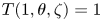
Throughout this section, we choose our domain to be bounded by $\rho =0$ and $\rho =1$
 and impose boundary conditions $T(0,\theta,\zeta )=0$
 and $T(1,\theta,\zeta )=1$
 .
7.1. Transport with one intact flux surface
In this section, we verify the lower (§ 3.1) and upper (§ 4.1) bounds on the transport in the presence of one intact flux surface. We will assume both of the bounding surfaces, $S_0$ and $S_{\infty }$
 , to be magnetic surfaces and the inequality (4.10) to be satisfied in the neighbourhood of each surface. In this case, the upper bound on the transport can be further reduced by assuming a trial function of the form,

where $z_1$ is the location of the interior flux surface.
The diffusion is minimised by $\delta _j = \ell _j (3 \epsilon )^{1/2}$ and


resulting in the upper bound,

To numerically test these bounds, we consider a model Hamiltonian which possesses magnetic surfaces at $\rho = 0$ , $\rho = 0.5$
 and $\rho = 1$
 ,

with $n/m = [1/10,1/5,3/10,2/5,3/5,7/10,4/5,9/10]$ . We take our boundaries to be at $\rho = 0$
 and $\rho = 1$
 and have an internal flux surface at $\rho = 0.5$
 . Thus, we can associate $\rho$
 with the coordinate $z$
 appearing in the trial function. We adjust the level of the perturbation amplitude, $\mathcal {E}$
 , to investigate the effect on the transport as it approaches the upper bound.
We can compute the length scales, $\ell _j$ , for the radial component of the field, which satisfy the inequality,

The maximum of the function

is numerically computed to be $f_{{\rm max}} \approx 54.7163$ such that

In the neighbourhood of $\rho = 0$ , $|B_{\rho }|/B \lesssim 0.5\mathcal {E} \rho f_{{\rm max}}$
 giving a length scale of $\ell _0 = 2/(\mathcal {E} f_{{\rm max}})$
 . Similarly, the length scales at $\rho = 0.5$
 and $\rho = 1$
 are given by $\ell _1 = 2 \sqrt {5}/(\mathcal {E} f_{{\rm max}})$
 and $\ell _{\infty } = 2 \sqrt {2}/(\mathcal {E} f_{{\rm max}})$
 .
We compute the numerical solution to the anisotropic diffusion equation (1.2)–(1.3) using a Fourier Galerkin discretisation in $\theta$ and $\zeta$
 and a fourth-order finite-difference radial discretisation. The resulting sparse linear system is solved with the PETSc library using the MUMPS package (Amestoy et al. Reference Amestoy, Duff, Koster and L'Excellent2001, Reference Amestoy, Buttari, L'Excellent and Mary2019) to compute the $LU$
 -factorisation. In figure 4 we present Poincaré sections of our model field at $\zeta = 0$
 in addition to the computed isotherms with $\epsilon = 10^{-6}$
 . At smaller values of the perturbation amplitude, we see the remnants of island chains in addition to barriers and chaotic regions. The isotherms conform to the structure of the separatrices of the island chains. We note that, as the perturbation amplitude is increased, the magnetic field becomes visually chaotic and the temperature gradient becomes localised near the magnetic surfaces, but away from these the isotherms display a remarkable degree of structure. For a moderately large perturbation amplitude, $\mathcal {E} = 0.1$
 , the field appears to be strongly stochasticised. Nonetheless, there remain several isotherms which conform to the remnants of secondary island structures near the barriers. Only in the case of the largest perturbation amplitude, $\mathcal {E} = 0.5$
 , do the pressure gradients become extremely localised near the boundaries. As the trial functions involve complete flattening of the temperature gradient over large regions, we expect to approach the upper transport bound only for sufficiently small $\epsilon$
 and sufficiently large $\mathcal {E}$
 , so that the field is strongly stochastic with dominantly parallel diffusion.
Numerical solutions of the anisotropic diffusion equation with $\epsilon = 10^{-6}$ are overplotted on the Poincaré section of the model magnetic field (7.1) with the displayed values of $\mathcal {E}$
 : (a) $\mathcal {E} = 0.01$
 , (b) $\mathcal {E} = 0.05$
 , (c) $\mathcal {E} = 0.1$
 and (d) $\mathcal {E} = 0.5$
 . For each plot, 50 equally spaced isotherms are displayed (red). The following resolution parameters were used: $m \leq 20$
 , $|n|\leq 20$
 , $N_{\rho }=250$
 ($\mathcal {E} = 0.01$
 ); $m \leq 20$
 , $|n|\leq 20$
 , $N_{\rho }=250$
 ($\mathcal {E} = 0.05$
 ); $m \leq 30$
 , $|n|\leq 30$
 , $N_{\rho }=600$
 ($\mathcal {E} = 0.1$
 ); $m \leq 5$
 , $|n| \leq 5$
 , $N_{\rho } = 10^{5}$
 ($\mathcal {E} = 0.5$
 ). Here $m$
 is the poloidal mode number, $n$
 is the toroidal mode number and $N_{\rho }$
 is the number of radial grid points.

In figure 5 we compare the numerical value of the diffusion with the upper and lower bounds for $\epsilon = 10^{-6}$ , $10^{-7}$
 and $10^{-8}$
 and several values of the perturbation amplitude $\mathcal {E}$
 . The lower bound is computed using the minimiser of the isotropic diffusion integral, $D_{{\rm lower}}[\tilde {T}] = ({\kappa _{\perp }}/{2}) \int _{\varOmega } |\boldsymbol {\nabla } \tilde {T}|^{2} \,{{\rm d}}V$
 , which yields $T_{{\rm lower}} = \rho (T_{\infty }-T_{0})$
 . For the smallest perturbation amplitude, the total diffusion is within an order of magnitude of the lower bound. As $\epsilon$
 decreases, parallel diffusion becomes more dominant, and the difference between $D$
 and $D_{{\rm lower}}$
 increases marginally. Only for the largest perturbation amplitude ($\mathcal {E} =0.5$
 ) does the total diffusion come within an order of magnitude of the upper bound. There are several factors controlling the difference between $D$
 and $D_{{\rm upper}}$
 . Given the finite value of $\kappa _{\perp }$
 , there remains a small temperature gradient between the interfaces. The diffusion is further reduced from the upper bound due to the sinusoidal variation of the radial field. Finally, there is a further slight reduction in the diffusion due to the small angular dependence of the isotherms.


In figure 6 we choose a specific value of the perturbation amplitude, $\mathcal {E} =0.5$ , and compare the numerical solution ($\epsilon = 10^{-6}$
 ) for the temperature profile averaged over $\theta$
 and $\zeta$
 to the trial function (7.4). We note that the numerical temperature profile is somewhat smoother than the trial function. Nonetheless, several of the features are captured, including the value of the temperature between the interfaces and the location of the strong gradient. We remark that the trial function coincides with the physical temperature profile only for very large perturbation amplitudes ($\mathcal {E} = 0.5$
 ), as significant poloidal and toroidal variation of the isotherms remain at $\mathcal {E} = 0.1$
 in addition to a widening of the temperature gradient length scale in comparison with the predicted $\delta _j$
 .
The numerical solution of the temperature profile (blue) averaged over $\theta$ and $\zeta$
 is compared with the trial function (red). The heat diffusion equation is solved with $\epsilon = 10^{-6}$
 for the magnetic field (7.1) with perturbation amplitude $\mathcal {E} = 0.5$
 . (a) The overall temperature profile, which exhibits strong variation in thin boundary layers at $\rho = 0$
 , $\rho = 0.5$
 and $\rho = 1$
 . These are magnified in (b)–(d).

7.2. Transport with continuously nested isotherms
In this section, we build upon the ideas presented above in § 5 and illustrate the construction of accurate trial functions for the temperature when a continuous family of isotherms can be approximated. The representation of the magnetic field and the boundary conditions are the same as that described in § 7. For the magnetic perturbation, we choose $\chi _{m,n}(\rho ) = \epsilon _{m,n} \rho ^{2} (\rho - 1 )^{2}$ , with $\epsilon _{2,1} = 3 \epsilon$
 , $\epsilon _{3,1} = \epsilon _{3,2} = \epsilon$
 and $\epsilon _{4,1}= \epsilon _{4,3} = \epsilon /2$
 for $\epsilon =-0.005$
 . These perturbations vanish on the boundary, and $\rho =0$
 and $\rho =1$
 are flux surfaces. A Poincaré plot of this field is shown in figure 7. In this section, we take $\epsilon =\kappa _\perp /\kappa _\parallel =10^{-7}$
 .
(a) Poincaré plot of the magnetic field shown in $(\rho,\theta )$ coordinates, the isotherms of the exact solution shown as black lines (left half only), and the selected QFM surfaces shown as blue lines (right half only). (b) Poincaré plot of the same magnetic field shown in $(\psi,\theta _s)$
 coordinates, and the isotherms of the numerically computed temperature shown as black lines (left half only). To a good approximation, the isotherms coincide with surfaces $\psi =const.$


We consider three trial functions that are constructed by first constructing a continuous set of surfaces, which are assumed to approximate isotherms and which we call trial isotherms, and which may be labelled by an arbitrary surface label, $\psi$ . For the first of the trial functions, we take the temperature profile to be given by the solution to the isothermal transport case. For the latter two of the trial functions, given the geometry of the trial isotherms, we solve (5.3) for the temperature profile. The accuracy of these trial functions is evaluated by constructing the ‘exact solution’ numerically.
Given that the boundaries of the domain are themselves assumed to be isotherms, the simplest construction of a family of trial isotherms is obtained by suitably interpolating between the boundaries. A particularly relevant interpolation is provided by the contours of the harmonic function $\nabla ^{2}T_{\rm iso}=0$ that equals $T_0$
 on $S_0$
 and $T_\infty$
 on $S_\infty$
 , as this corresponds to the isotropic diffusion case as discussed in § 3.1. Thus, for our first family of trial isotherms, we take the isotherms of the solution that is obtained when the enhanced parallel transport is ignored, which is obtained when $\epsilon =\kappa _\perp /\kappa _\parallel =1$
 . For the simple geometry considered here, this solution is $T_{\rm iso}(\rho,\theta,\zeta )=\rho$
 , which has contours $\rho =const$
 . Substituting this function directly into the diffusion integral (that is, without changing the geometry of the isotherms and without changing the temperature profile), we obtain $D[T_{\rm iso}]=213.178$
 .
For the second trial function we assume that the isotherms remain coincident with those of the isothermal solution (in this case, surfaces $\rho =const.$ ), but we now solve (5.3) with $\epsilon =\kappa _\perp /\kappa _\parallel =10^{-7}$
 to obtain the temperature profile. Inserting the trial function for the temperature thus obtained, which we call $\tilde T_{\rm iso}$
 , into the diffusion integral we obtain $D[\tilde T_{\rm iso}]=89.5803$
 .
More accurate trial functions can be obtained if, by some means, more accurate approximations to the isotherms can be constructed. Given that, as $\kappa _\parallel$ becomes larger (or as $\kappa _\perp$
 becomes smaller), it is the spatial structure of the magnetic field that primarily determines transport. It becomes increasingly plausible that we can set more accurate (i.e. lower) upper bounds on transport across non-integrable magnetic fields by identifying structures that are invariant or almost-invariant under the magnetic field-line flow, such as KAM surfaces and cantori.
A practical numerical approach for constructing invariant and almost invariant surfaces is provided by the construction of (weighted) QFM surfaces (Dewar et al. Reference Dewar, Hudson and Price1994; Hudson & Suzuki Reference Hudson and Suzuki2014). An algorithm for constructing these surfaces is described in Appendix A. A set of QFM surfaces, defined by their periodicities $\boldsymbol {p}/\boldsymbol {q}=\{ 0/ 1$ , $1/ 10$
 , $1/ 9$
 , $1/ 8$
 , $2/ 15$
 , $1/ 7$
 , $3/ 20$
 , $2/ 13$
 , $3/ 19$
 , $1/ 6$
 , $3/ 17$
 , $2/ 11$
 , $3/ 16$
 , $1/ 5$
 , $3/ 14$
 , $2/ 9$
 , $3/ 13$
 , $1/ 4$
 , $3/ 11$
 , $5/ 18$
 , $2/ 7$
 , $5/ 17$
 , $3/ 10$
 , $4/ 13$
 , $1/ 3$
 , $4/ 11$
 , $3/ 8$
 , $5/ 13$
 , $2/ 5$
 , $5/ 12$
 , $3/ 7$
 , $7/ 16$
 , $4/ 9$
 , $5/ 11$
 , $1/ 2$
 , $6/ 11$
 , $5/ 9$
 , $9/ 16$
 , $4/ 7$
 , $7/ 12$
 , $3/ 5$
 , $8/ 13$
 , $5/ 8$
 , $7/ 11$
 , $2/ 3$
 , $7/ 10$
 , $12/ 17$
 , $5/ 7$
 , $8/ 11$
 , $3/ 4$
 , $7/ 9$
 , $11/ 14$
 , $4/ 5$
 , $9/ 11$
 , $5/ 6$
 , $11/ 13$
 , $6/ 7$
 , $13/ 15$
 , $7/ 8$
 , $8/ 9$
 , $9/ 10$
 , $1/ 1 ) \}$
 , are shown as the blue curves in the left figure in figure 7. (How these periodicities were chosen is described further in the following.)) These surfaces are taken as coordinate surfaces to construct the coordinate mapping $\boldsymbol {x}(\psi,\theta _s,\zeta )$
 , where $\psi$
 labels the enclosed toroidal flux and $\theta _s$
 is a straight pseudo-field-line angle. An interpolation between the surfaces provides a continuous coordinate framework for non-integrable magnetic fields, which reduces to straight-field-line coordinates where flux surfaces exist. Much of the field-line dynamics that remains invariant after perturbation can be incorporated into the coordinates, and we call these coordinates chaotic coordinates (Hudson & Suzuki Reference Hudson and Suzuki2014). The Poincaré plot of the same magnetic field as shown in the left plot of figure 7 is shown in chaotic coordinates in the right plot of figure 7.
We take as our third family of trial isotherms to be the QFM surfaces and their radial interpolates, where the temperature profile is given by the solving (5.3). For the trial function, $T=T_{\boldsymbol {p}/\boldsymbol {q}}$ , thus obtained, the diffusion is $D[T_{\boldsymbol {p}/\boldsymbol {q}}] = 24.8809$
 .
We may compute the exact solution using a mixed finite-difference Fourier representation for the temperature, $T(\rho _i,\theta,\zeta )=\sum _{m=0}^{M}\sum _{n=-N}^{N}T_{m,n,i} \cos (m\theta -n\zeta )$ including Fourier modes up and including $M=10$
 and $N=10$
 with a second-order finite-difference approximation for the radial derivatives and $256$
 radial grid points, and minimise $D[T]$
 with respect to the $T_{m,n,i}$
 . The numerically constructed temperature, $T_e$
 , which for convenience we consider to be the exact solution, is shown as the black curves in the right-hand figure in figure 7. Note that, visually, the isotherms coincide with coordinate surfaces to a very good approximation. With the accurate approximation of the exact temperature, $T_e$
 , obtained numerically, the diffusion is $D[T_e]=22.8721$
 .
We can compare the values of $D[T_{\rm iso}]$ , $D[\tilde T_{\rm iso}]$
 and $D[T_{\boldsymbol {p}/\boldsymbol {q}}]$
 to $D[T_{e}]$
 . We see that $(D[T_{\rm iso}]-D[\tilde T_{\rm iso}])/(D[T_{\rm iso}]-D[T_e])\approx 0.65$
 , which means that $65\,\%$
 of the total possible reduction of the diffusion integral (starting from the isothermal solution) is achieved merely by solving for the isothermal solution to obtain a family of trial isotherms and then solving (5.3) for the temperature profile. (Note that solving for the isothermal solution is a much simpler numerical task than solving for the exact solution, because the isothermal solution only depends on the geometry of the boundary and not on the magnetic field itself.) For the trial function based on the QFM surfaces and their interpolates, and solving (5.3), we obtain $(D[T_{\rm iso}]-D[T_{\boldsymbol {p}/\boldsymbol {q}}])/(D[T_{\rm iso}]-D[T_e])\approx 0.99$
 . Based on this, the trial function based on chaotic coordinates and solving (5.3) yields an improvement of $99\,\%$
 in the sense that over $99\,\%$
 of the total possible reduction of the diffusion integral resulting from including the strong parallel transport has been achieved. It is much faster to construct QFM surfaces than to solve the anisotropic diffusion equation numerically.
The selection of the QFM surfaces requires some explanation. QFM surfaces are characterised by their periodicity, and we may distinguish the following cases.
(i) For $(p,q)$
 that are low-order rationals, e.g. $p/q=1/2, 1/3, \ldots,$ because the low-order islands are typically larger than the high-order islands and because the $(p,q)$ QFM surface pass through the $(p,q)$ island, we may expect that low-order $(p,q)$ QFM surfaces are isotherms because the temperature tends to flatten inside the larger islands.
(ii) For $(p,q)$
that are high-order rationals that approximate a strongly irrational number, then the QFM surface is an excellent approximation to the KAM surface if it exists, or if it does not the QFM surface effectively ‘fills in the gaps’ in the cantorus. In both cases, because complete barriers and partial barriers to magnetic field-line transport are likely to be isotherms, then these QFM surfaces are likely to be isotherms too.(iii) A particularly interesting case is when $p/q$
is a high-order rational that approximates a low-order rational, e.g. $p/q=101/200$. In this case, the QFM surface lies just outside of the low-order island separatrix, and whether this QFM surface is an isotherm depends on how large the low-order island is and on $\kappa _\perp$.


The question thus arises: which QFM surfaces are most likely to coincide with isotherms? The answer partly depends on the structure of the non-integrable magnetic field, namely whether the magnetic field is completely integrable, nearly integrable or strongly chaotic, and also on how much the parallel transport dominates the perpendicular. A practical algorithm, used in this study, is provided by constructing successively sophisticated trial functions and evaluating the diffusion integral. If the diffusion integral decreases, then the trial function is a more accurate approximation of the true solution.
We start from a trial function, $T_{\boldsymbol {p}/\boldsymbol {q}}$ , built on a family of trial isotherms constructed by an interpolation of a selection of a few, low-order QFM surfaces (in this example we may begin with the $\boldsymbol {p}/\boldsymbol {q} = \{0/1, 1/2, 1/1\}$
 set of QFM surfaces) and solve for the temperature profile given in (5.3), and then compute $D[T_{\boldsymbol {p}/\boldsymbol {q}}]$
 . Next, we construct a refined trial function by augmenting the previous selection of QFM surfaces by, typically, adding mediants, to obtain $(p_{i}+p_{i+1})/(q_{i}+q_{i+1})$
 , to obtain, for example, the set of $\boldsymbol {p}/\boldsymbol {q} = \{0/1, 1/2, 1/2, 2/3, 1/1\}$
 QFM surfaces, recompute the interpolation to construct the family of trial isotherms, re-solve (5.3) and then recompute the diffusion. Adding more and higher-order QFM surfaces effectively adds more of the fractal structure of the magnetic field to the trial function. If the diffusion integral for the refined trial function decreases, then a better (lower) upper bound on transport has been obtained and the refined trial function is a better approximation to the exact solution. Additional mediants can be included, one at a time if need be, until the diffusion integral no longer decreases, and this may occur when the scale length of the QFM surfaces is smaller than the scale length of the true solution, which is in part set by $\epsilon =\kappa _\perp /\kappa _\parallel$
 . In this fashion, we may systematically improve our estimate for the global temperature solution, and in so doing identify the most important barriers to anisotropic transport for non-zero $\epsilon$
 in non-integrable magnetic fields. There are other potential algorithms for identifying the most suitable QFM surfaces to be used as trial isotherms, and we shall explore these ideas in future work.
8. Discussion
Magnetic fields with chaotic field lines can possess a surprising degree of structure, which is not readily visible in a Poincaré puncture plot but becomes apparent when one for instance considers anisotropic transport processes. In such situations, traditional estimates (Rechester & Rosenbluth Reference Rechester and Rosenbluth1978; Kadomtsev & Pogutse Reference Kadomtsev and Pogutse1979; Krommes et al. Reference Krommes, Oberman and Kleva1983) of the ‘effective’ diffusion coefficient are unreliable and one must instead take the detailed geometry of the magnetic field into consideration. KAM surfaces, and remnants thereof, act as barriers to the diffusion, and their effect can be quantified through rigorous upper and lower bounds on the net transport. A more restrictive upper bound can be found whenever the isothermal surfaces can be guessed to good accuracy. Such surfaces can be constructed in natural by using ‘chaotic coordinates’, which also find wide application in other parts of plasma physics and in Hamiltonian dynamical systems.
Acknowledgements
One of the authors (PH) would like to acknowledge the hospitality of the Department of Astrophysical Sciences of Princeton University and PPPL, where much of this work was performed. It was supported by a grant from the Simons Foundation/SFARI (560651, AB). This work was supported in part by DOE Contract No. DEAC02–76CH03073.
Editor Peter Catto thanks the referees for their advice in evaluating this article.
Declaration of interests
The author report no conflict of interest.
Appendix A. Area-constrained extremising curves and QFM surfaces
Here we present an algorithm for constructing rational, $p/q$ , QFM surfaces. The calculation is performed in toroidal coordinates, $\boldsymbol {x}(\rho,\theta,\zeta )$
 . After a selection of QFM surfaces have been constructed, the QFM surfaces can themselves be used as coordinate surfaces. We seek periodic curves, ${{\mathcal {C}}}$
 , that are stationary points of the constrained-area action integral (Hudson & Suzuki Reference Hudson and Suzuki2014),

where $\alpha \in [0,2{\rm \pi} /q]$ is given and $\nu$
 is a Lagrange multiplier. Note that

is the ‘area’ under the $\theta (\zeta )$ curve, and dividing by $2{\rm \pi} q$
 and subtracting $p{\rm \pi}$
 is done for convenience. The parameter $\alpha$
 will later be used as a field-line label. An arbitrary periodic trial curve is described by


where the periodicity of the curve is defined by the integers $p$ and $q$
 , and the independent degrees of freedom that describe the curve geometry are the quantities $\rho ^{c}_n$
 , $\rho ^{s}_n$
 , $\theta ^{c}_n$
 , and $\theta ^{s}_n$
 for $n=0, 1, \ldots, N$
 , where $N$
 is the chosen Fourier resolution. Note that $\rho (\zeta +2{\rm \pi} q)=\rho (\zeta )$
 and $\theta (\zeta +2{\rm \pi} q)=\theta (\zeta )+2{\rm \pi} p$
 . The vector potential can be written $\boldsymbol {A} = A_\rho \boldsymbol {\nabla } \rho + A_\theta \boldsymbol {\nabla } \theta + A_\zeta \boldsymbol {\nabla } \zeta$
 . (Note that in the following, the vector potential itself is not actually required.)
Allowing for variations $\delta \rho (\zeta )$ and $\delta \theta (\zeta )$
 in the trial curve, and $\delta \nu$
 in the Lagrange multiplier, the variation in ${{\mathcal {S}}}$
 is

where


where $B^{\rho } = \boldsymbol {B}\boldsymbol {\cdot }\boldsymbol {\nabla } \rho$ , $B^{\theta } = \boldsymbol {B}\boldsymbol {\cdot }\boldsymbol {\nabla } \theta$
 and $B^{\zeta } = \boldsymbol {B}\boldsymbol {\cdot }\boldsymbol {\nabla } \zeta$
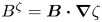 , $\sqrt g$
 is the coordinate Jacobian, and $\dot \rho$
 and $\dot \theta$
 are the (total) derivatives of $\rho (\zeta )$
 and $\theta (\zeta )$
 , respectively.
We can find extrema by identifying zeros of the gradient,


together with (A8). For systems with shear, it is possible to invert (A6) to obtain $\rho =\rho (\dot \theta,\theta,\zeta )$ , and the result can be used to eliminate $\rho (\zeta )$
 as an independent degree of freedom; however, doing so complicates the algorithm. A straight ‘pseudo-field-line’ angle is constructed along each extremal curve, $\theta _s = \alpha + p \zeta / q$
 . By varying $\alpha \in [0,2{\rm \pi} /q]$
 , we may construct a family of periodic curves that together comprise the QFM surface.
Each QFM surface can be labelled by the enclosed toroidal flux,

where ${{\mathcal {S}}}$ is the surface on the $\zeta =0$
 plane bounded by $\theta =0$
 , $\theta =2{\rm \pi}$
 , $\rho =0$
 and the QFM surface. A Fourier decomposition of $\rho (\psi,\theta _s,\zeta )$
 and $\lambda (\psi,\theta _s,\zeta ) \equiv \theta - \theta _s$
 can be computed, and a continuous coordinate system can, thus, be constructed by an interpolation of the Fourier harmonics of $\rho (\psi,\theta _s,\zeta )$
 and $\lambda (\psi,\theta _s,\zeta )$
 in terms of toroidal flux.


 Open access

