


1. Introduction
In the Southern Ocean, heavy snow accumulation can depress sea ice below the water level, leading to flooding and the formation of brine-saturated slush layers (Fichefet and Maqueda, Reference Fichefet and Maqueda1999; Massom and others, Reference Massom, Eicken, Haas, Jeffries, Drinkwater and Allison2001). As these slush layers freeze, saline snow-ice forms at the base of the snowpack (Takizawa, Reference Takizawa1985; Jeffries and others, Reference Jeffries, Krouse, Hurst-cushing and Maksym2001; Maksym and Markus, Reference Maksym and Markus2008; Komarov and others, Reference Komarov2025). Even in cold winter temperatures, these layers can contain concentrated liquid brine, which influences the thermodynamic and electromagnetic properties of the snow (Crocker, Reference Crocker1984; Drinkwater and Crocker, Reference Drinkwater and Crocker1988; Barber and others, Reference Barber, Reddan and LeDrew1995; Barber and others, Reference Barber, Iacozza and Walker2003; Geldsetzer and others, Reference Geldsetzer, Langlois and Yackel2009; Stroeve and others, Reference Stroeve, Nandan, Willatt, Dadic, Rostosky and Schneebeli2022).
However, the migration of saline water through snow is a complex process controlled by multiple factors, including air temperature, volume and salinity of liquid, initial snow properties and stratigraphy, which vary depending on weather conditions during and after snow accumulation (Sturm and others, Reference Sturm, Morris and Massom1998; Sturm and Massom, Reference Sturm and Massom2009; Komarov and Sturm, Reference Komarov and Sturm2023). Metamorphic processes within the snowpack can transform existing layers, resulting in snow compaction and the development of coarse-grained layers composed of large faceted and depth hoar crystals near the snow–ice interface. In comparison to the fine-grained wind-slab layers, such coarse-grained layers have different pore sizes and shapes that influence capillary action and liquid retention capacity (Coléou and others, Reference Coléou, Xu, Lesaffre and Brzoska1999; Yamaguchi and others, Reference Yamaguchi, Katsushima, Sato and Kumakura2010; Lombardo and others, Reference Lombardo, Fees, Kaestner, van Herwijnen, Schweizer and Lehmann2025). When a coarse-grained layer is overlain by a fine-grained wind slab (WS), this could lead to the development of a capillary barrier at their interface and preferential pooling of the liquid.
This study expands on previous findings (Komarov and others, Reference Komarov2025) that investigated the effects of snow microstructure on liquid capillary wicking and runoff under semi-controlled conditions and demonstrated that snow grain type and density have a pronounced effect on the height of liquid wicking, runoff volume, snow compaction rates and salt concentrations. In coarse-grained samples, capillary forces and liquid retention capacities were weaker compared to fine-grained snow and, as a consequence, wicking height was smaller. Separation of the initial brine-saturated slush layer after freezing into two sublayers (snow-ice and brine-wetted layer) was observed in all samples regardless of snow type.
In the current study, we examine how variations in liquid volume and salinity influence its wicking in snow. The present manuscript builds upon the same experimental infrastructure and methodology, adding a second layer of inquiry focused on liquid volume and salinity. Furthermore, this study explores the role of snow stratigraphy in brine migration, snow-ice formation and brine distribution. Previous research on freshwater infiltration suggests that distinct snow layers can act as capillary barriers, leading to the formation of lenses, percolation columns and basal ice layers (Colbeck, Reference Colbeck1974; Avanzi and others, Reference Avanzi, Hirashima, Yamaguchi, Katsushima and De Michele2016; Wever and others, Reference Wever2020). However, the effect of snow stratification on the upward migration of saline liquid remains poorly understood.
This study aims to determine how the volume and salinity of infiltrating seawater, along with the structural characteristics of the snowpack, influence saline water and brine wicking and redistribution within the snow cover.
2. Materials and methods
We selected several types of natural snow (Fig. 1 and Table 1), each characterized by distinctly different grain sizes and shapes: wind-packed rounded grains, faceted crystals (FC) and melt-form clustered rounded grains (Fierz and others, Reference Fierz2009). Hereinafter, we refer to these types as WS, FC and melt-freeze clusters (MF), respectively. Snow crystals from these three snow types were collected along a transect at the study site and then filtered through 1-, 2- and 5-mm sieves. We used a magnifying glass and a gridded crystal card to characterize the snow types.
Map of the snow ‘farm’ of (a) the main experiment (volume and salinity) and (b) the side experiment (snow stratigraphy). Samples A-D1 and A-D2 in plastic tubes, wicked 50 and 100 mL of 53.4 ppt brine, respectively. Samples A-D3 wicked 50 mL of 30.1 ppt liquid. Green squares A–D4 represent brine-free reference snow samples. A1–A4—soft wind slab; B1–B4—hard wind slab; C1–C4—faceted crystals; D1–D4—melt-freeze clusters (see Table 1). Samples E1–E3 had different stratigraphy, and each one wicked 100 mL of 53.4 ppt brine. Examples of samples from (c) the main experiment and (d) the side experiment.

1 Long description
Four parts labeled a, b, c and d. Part s a and b are grid-based schematics showing the spatial layout of snow sample positions and their assigned experimental conditions. Part a is titled as the main experiment and contains two rows of samples. The first row is labeled WS1 and contains samples A1, A2, A3 and A4. The second row is labeled WS2 and contains samples B1, B2, B3 and B4. To the right of part a, part b shares the same grid structure and contains two rows. The first row is labeled FC with samples C1, C2, C3 and C4. The second row is labeled MF with samples D1, D2, D3 and D4. A vertical label on the far right reads, location of temperature logger. Both parts a and b share the same column-level volume and salinity labels printed above the grid. The four columns carry the following values from left to right: Vol 50 ml and Sal 53.4 ppt, then Vol 100 ml and Sal 53.4 ppt, then Vol 50 ml and Sal 30.1 ppt, then Vol 0 ml and Sal 0 ppt. Samples in the first three columns of each row are shown as brine samples. Samples in the fourth column of each row, which are A4, B4, C4 and D4, are shown as brine-free reference samples. Part b is the side experiment and shows three columns each labeled with Vol 100 ml and Sal 53.4 ppt. The single row contains samples E1, E2 and E3. Below the grid, the three column positions are labeled WS slash MF, WS slash FC and WS slash MF slash WS. Part c is a photograph showing a plastic tube labeled A1 embedded in a white material. Pink liquid is visible at the lower portion of the tube, with measurement markings on its side. Part d is a photograph showing a flat rectangular sample labeled E3, with a ruler placed alongside it showing measurements up to approximately 13 centimeters. Pink liquid is visible at the base of the sample.
Type, grain size and initial average densities of snow samples. CV is coefficient of variation.

Table 1 Long description
Four snow sample groups list indexes, snow type, grain size in millimeters, snow density in kilograms per cubic meter, standard deviation in kilograms per cubic meter, and CV. Indexes A1 to A4 are Wind Slab Soft, WS1, with grain size 0.2 to 0.5, density 370, standard deviation 6, and CV 0.02. Indexes B1 to B4 are Wind Slab Hard, WS2, with grain size 0.2 to 0.5, density 430, standard deviation 12, and CV 0.03. Indexes C1 to C4 are Faceted Crystals, FC, with grain size 0.5 to 2, density 305, standard deviation 6, and CV 0.02. Indexes D1 to D4 are Melt Freeze Clusters, MF, with grain size 0.2 to 5, density 465, standard deviation 18.5, and CV 0.04.
To study the effect of liquid volume and salinity on its wicking and runoff, the filtered snow was then used to fill 20-cm-high transparent plastic tubes with a diameter of 8 cm to produce homogeneous samples. Altogether, 16 tubes were filled with sampled snow: the first 8 tubes were filled with WS snow of small rounded grains, the next 4 with FC and the last 4 with MF. Snow was manually compressed using a round plastic plate with an 8-cm diameter and a flat bottom surface to achieve desired the densities typical of snow types found in sea-ice environments (Sturm and Massom, Reference Sturm and Massom2009). All samples were placed at the field site and left for 2 days under subzero temperatures to produce sintered snow samples. The transparent tubes enabled us to observe changes in brine migration daily. Samples were weighed and numbered, and the snow density of each sample was calculated. The bulk density, standard deviation and coefficient of variation (CV) were calculated (Table 1).
Each sample was placed in a previously prepared snow ‘farm’, a container built of snow to protect the samples from melting, wind and rapid changes in air temperature. Each row of the farm hosted four tubes. In the farm, samples were placed into plastic trays filled with a liquid solution of known concentration (30.1 and 53.4 ppt) and volume (50 and 100 mL) (Fig. 1a). When the solution was added to the samples, the farm’s bottom surface temperature was −7°C and the input liquid temperature was −1°C. An exception was made for samples A-D4, which were left brine-free as reference samples. This approach enabled comparison of the compaction rates between the samples with and without brine. To trace liquid migration through the snow, we added Rhodamine WT dye (Mallett and others, Reference Mallett2024) to the initial solution.
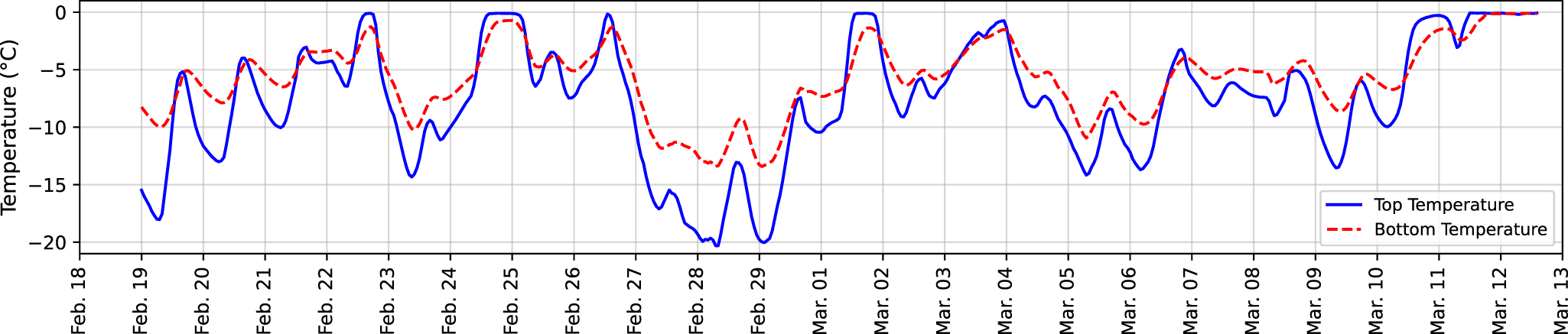
Identically to Komarov and others (Reference Komarov2025), the salinity of initial liquid, melted snow and brine runoff was measured with the Orion Star 212A conductivity meter (0.01 ppt resolution; ±0.5% accuracy) calibrated at three points with liquid solutions of 1413, 12.88 and 99.99 mS cm−1. To measure the temperature inside the farm, we combined manual (Testo 720, accuracy ± 0.5°C) and automatic (Campbell Scientific CR1000/T109, accuracy ± 0.06%) temperature sensors. The bottom sensor was placed 0.5 cm above the ground surface and measured the temperature at the very bottom of the C4 cell (Fig. 1a). The upper logger was installed at a height of 20 cm within the same cell. We also acquired hourly data from the nearby Winnipeg airport weather station to characterize the variability in air temperature, precipitation and wind speed during the field experiment. The samples were continuously monitored for 23 days, from 19 February to 12 March 2024 and followed the same protocol as Komarov and others (Reference Komarov2025).
A supplementary experiment was conducted to assess the effect of snow stratigraphy on brine wicking and runoff (Fig. 1b). From the same filtered snow, we produced snow samples with three different snow layerings: (i) WS overlying melt-freeze layers (E1), (ii) WS overlying faceted crystals (E2) and (iii) alternating WS and melt-freeze thin layers (E3). The samples had a rectangular shape with a 10 × 10 cm (100 cm2) base and a height of 13–15 cm. To each sample, we added 100 mL of 53.4 ppt brine and continuously monitored brine wicking for 20 days, from 21 February to 11 March 2024. The volume of liquid was twice larger than in samples A-D1 and A-D3 from the main experiment, where we added liquid to the samples in plastic tubes with a base area of 50 cm2. In other words, these samples received 1 mL of liquid per 1 cm2 of base area. As before, we measured the snow height, wicking height and changes in snow stratigraphy. However, we measured snow density, salinity and snow water equivalent only twice: before adding liquid and on the last day of the experiment.
3. Results
3.1. Weather conditions
The daily averaged air temperature measured at Winnipeg Airport exhibited considerable variability, ranging from − 21.2°C to +2.5°C during the experiment (19 February to 12 March). The mean air temperature throughout the experiment was −8.1°C. At the bottom of the experimental ‘farm’, the average temperature was −5.7°C, which was 2°C warmer than at the top. The minimum recorded temperature was −13.5°C at the bottom and −20°C at the top (Fig. 2), while the maximum temperature at the bottom remained just below freezing at −0.1°C. However, at the top, the temperature exceeded freezing at +0.02°C on the final day of the experiment. Although a temperature gradient was present within the samples, it was less than 0.1°C cm−1 and was not strong enough to cause kinetic growth and thus impact the snow stratigraphy. It remained below zero at both levels until the last day of the experiment. The snow did not reach temperatures above zero, as after each measurement the farm was carefully covered with an insulating layer on the top and all four sides to prevent any melting during the short-term thaw periods in February and early March. This allowed us to avoid surface melting of the samples. The absence of surface melt was further confirmed by destructive sampling, performed semi-daily during the main experiment (Komarov and others, Reference Komarov2025). No traces of liquid water percolation were observed in the upper sections of the samples until 12 March.
The temperature at the top and the bottom of the C4 cell (see Fig. 1) measured at 15-min intervals (Campbell Scientific CR1000/T109 temperature logger).

When saline water and brine were added to the samples, the entire volume was wicked by snow within few minutes and reached a height of nearly 2.5 cm, developing a layer of saturated slush. During the night, when the temperature dropped, this slush layer froze, and hard, dense snow-ice layer developed within few hours after we added liquid at the base. However, we did not measure this process in detail, as the subsequent measurements were made the next day, when the snow-ice layer was already present and a brine-wetted layer developed above it. Compared to solid snow-ice, this brine-wetted layer (Takizawa, Reference Takizawa1985) retained a snow-like structure and was significantly less dense (∼38%; 520 kg m−3 vs. 840 kg m−3) and less saturated compared to slush or snow ice (Komarov and others, Reference Komarov2025). We believe this second layer developed due to additional wicking of concentrated brine rejected from the freezing slush and growing snow-ice layer. This process is discussed in more detail in Komarov and others (Reference Komarov2025). After freezing, this hard, dense snow-ice layer at the bottom of the snowpack remained until the end of the experiment, while brine migration continued.
3.2. The impact of liquid volume
The temporal evolution of saline layers after adding different volumes of liquid is shown in Fig. 3. Numerical data are provided in Supplementary Appendix 1. The average thickness of the snow-ice layer across all four snow types, after adding 50 and 100 mL of 53.4 ppt brine, was 3.2 and 4.5 cm, respectively, reflecting a 40% increase. The thickness of the brine-wetted layer was 3.2 and 3.3 cm, showing only a 4% increase (less than the accuracy of the measurements). The total thickness of the brine-affected layers was 6.4 and 7.8 cm, corresponding to a 22% increase (Fig. 3). Thus, while the liquid volume was doubled, the resulting difference in the thickness of the brine-affected layers was much smaller. Furthermore, the change in snow-ice thickness was notably larger than that of the brine-wetted layers, which remained almost unchanged regardless of the brine volume.
Variations in the thickness of snow-ice, brine-wetted and fresh snow layers across the four snow types during the 23 days of the experiment are shown after adding 50 mL (solid line) and 100 mL (dotted line) of 53.4 ppt brine. The black triangle on the x-axis represents the date of brine runoff after adding 50 mL, while the black circle marks the date of brine runoff after adding 100 mL.

Figure 3 Long description
A showing the title, WS1 53.4 ppt: 50 ml vs 100 ml. The horizontal axis shows dates from Feb. 19 to Mar. 12. The vertical axis label is Snow Height (cm), ranging from 0.0 to 20.0. Two upper lines run near 20.0 at Feb. 19 and decline to about 16.0 to 17.0 by Mar. 12, with one line drawn solid and one line drawn dotted. A stacked filled area rises from about 2.0 to 3.0 at Feb. 19 to about 6.0 to 7.0 by late February, then stays near about 6.0 to 7.0 through Mar. 12. A lower dotted line within the filled region rises from about 3.0 at Feb. 19 to about 6.0 by around Mar. 01, then stays near about 5.0 to 6.0 through Mar. 12. A second dotted line above the filled region rises from about 4.0 at Feb. 19 to about 9.0 to 10.0 by late February, then stays near about 9.0 through Mar. 12. Two markers appear on the x axis: a filled circle at Feb. 24 and a triangle at Feb. 28. B showing the title, WS2 53.4 ppt: 50 ml vs 100 ml. The horizontal axis shows dates from Feb. 19 to Mar. 12. The vertical axis label is Snow Height (cm), ranging from 0.0 to 20.0. Two upper lines start near 20.0 at Feb. 19 and decline, with one line drawn solid and one line drawn dotted. By Mar. 12, the solid line is near about 15.0 and the dotted line is near about 13.0. A stacked filled area rises from about 2.0 to 3.0 at Feb. 19 to about 8.0 to 9.0 by around Feb. 26, then stays near about 8.0 to 9.0 through Mar. 12. A lower dotted line within the filled region rises from about 4.0 at Feb. 19 to about 6.0 by around Mar. 07, then is near about 5.0 to 6.0 through Mar. 12. A second dotted line above the filled region rises from about 4.0 at Feb. 19 to about 10.0 by around Feb. 24, then drops to about 2.0 to 3.0 by around Feb. 26. Two markers appear on the x axis: a filled circle at Feb. 24 and a triangle at Mar. 11. C showing the title, FC 53.4 ppt: 50 ml vs 100 ml. The horizontal axis shows dates from Feb. 19 to Mar. 12. The vertical axis label is Snow Height (cm), ranging from 0.0 to 20.0. Two upper lines start near 20.0 at Feb. 19 and decline, with one line drawn solid and one line drawn dotted. By Mar. 12, the solid line is near about 14.0 and the dotted line is near about 12.5. A stacked filled area rises from about 2.0 at Feb. 19 to about 6.0 to 7.0 by early March, then stays near about 6.0 to 7.0 until Mar. 11 and drops to about 3.0 by Mar. 12. A lower dotted line within the filled region stays near about 3.0 to 4.0 from Feb. 19 through early March, then rises to about 6.0 by around Mar. 11 and drops to about 3.0 by Mar. 12. A second dotted line above the filled region rises from about 5.0 at Feb. 19 to about 8.0 by around Feb. 22, then stays near about 8.0 through Mar. 11 and rises to about 9.0 by Mar. 12. Two markers appear on the x axis: a filled circle at Feb. 24 and a triangle at Feb. 28. D showing the title, MF 53.4 ppt: 50 ml vs 100 ml. The horizontal axis shows dates from Feb. 19 to Mar. 12. The vertical axis label is Snow Height (cm), ranging from 0.0 to 20.0. Two upper lines start near 20.0 at Feb. 19 and decline, with one line drawn solid and one line drawn dotted. By Mar. 12, the solid line is near about 14.0 and the dotted line is near about 12.5. A stacked filled area rises from about 4.0 at Feb. 19 to about 7.5 to 8.0 by around Feb. 26, then stays near about 7.5 to 8.0 through Mar. 12. A lower dotted line within the filled region rises from about 4.0 at Feb. 19 to about 6.0 by around Mar. 07, then drops to about 3.0 by Mar. 12. A second dotted line above the filled region rises from about 6.0 at Feb. 19 to about 8.0 by around Feb. 21, then stays near about 8.0 through Mar. 09 and rises to about 9.0 by Mar. 12. Two markers appear on the x axis: a filled circle at Feb. 24 and a triangle at Feb. 28.
Simultaneously, a distinct difference was observed in the thickness of the snow layer above the brine-affected layers and in the total thickness of the snow sample. In samples with a smaller volume of brine, the thickness of the fresh snow layer was, on average, 30% greater compared to samples with a larger brine volume (11.4 cm vs. 8.7 cm). The total height of the snow sample with the larger brine volume was, on average, 7% smaller than that of the sample with less brine (16.5 cm vs. 17.7 cm), indicating that snow compaction was more pronounced in samples with more brine (Fig. 3).
The influence of brine volume on the thickness of the snow-ice and brine-wetted layers was, however, dependent on snow type (Fig. 3), which is consistent with previous findings (Komarov and others, Reference Komarov2025). In the WS1 and WS2 samples, the volume of added brine had a stronger effect on the thickness of the brine-wetted layers, compared with the larger-grained FC and MF samples, but had similar impacts on the thickness of the snow-ice layer. Doubling the brine volume had an overall larger impact on the height of the brine-affected (dotted line vs. solid line in Fig. 3) layers for the WSs (26–33%) than for the FC (18%) and MF (13%).
Analysis of brine runoff revealed that in samples with a larger volume of brine, runoff occurred earlier than in samples with less brine. This difference ranged from 2 days (FC, MF) to 5 days (WS1) and up to 14 days (WS2). Brine runoff from samples with 100 mL of brine was observed almost simultaneously across all snow types (on days 6–8 of the experiment). However, for samples with 50 mL of liquid, runoff began earlier in FC and MF samples (day 8) compared to WS1 (day 11) and WS2 (day 22). Our observations further indicate that the volume of runoff depends on the liquid volume added. For samples with 50 mL of brine, the volume of brine runoff was on average 50% smaller compared to samples with 100 mL, regardless of the snow type. The salinity of brine runoff from samples with a larger volume of brine was on average 20% higher compared to those with a smaller volume, likely due to earlier brine runoff from the larger-volume samples.
The brine runoff concentration was lower than that of the initial brine, indicating dilution by the melting snow within the snow-ice and brine-wetted layers. Additionally, it was observed that the snow salinity at the end of the experiment (after brine runoff) was higher in the snow-ice layer compared to the brine-wetted layer, regardless of snow type or brine volume (10–15 ppt vs. 5–7 ppt). However, more detailed experiments are needed to investigate this aspect further.
3.3. The impact of liquid salinity
The temporal evolution of saline layers after adding liquid of different salinity is shown in Fig. 4. Numerical data are provided in Supplementary Appendices 1 and 3. The average thickness of the snow-ice layer across all samples (averaged over the four snow types) after adding 50 mL of 30.1 and 53.4 ppt liquid was 2.6 and 3.2 cm, respectively, reflecting a 20% increase for the higher salinity content. The thickness of the brine-wetted layer was 2.7 cm for 30.1 ppt liquid and 3.2 cm for 53.4 ppt brine, showing a 17% increase. The total thickness of the brine-affected layers was therefore 5.4 and 6.4 cm, respectively, showing an 18% increase. These results suggest the difference in brine salinity does not play a large role in the thickness of the brine-affected layers (Fig. 4; Supplementary Appendices 1 and 2).
Variations in the thickness of snow-ice, brine-wetted, and fresh snow layers across the four snow types during the 23 days of the experiment are shown after adding 50 mL of 30.1 ppt (solid line) and 53.4 ppt (dotted line) liquid. The black triangle on the x-axis indicates the date of brine runoff after adding 30.1 ppt liquid, while the black circle represents the date of brine runoff after adding 53.4 ppt brine.

Figure 4 Long description
The multi-line graphs compare snow height changes over time for four snow types: WS1, WS2, FC and MF, with two salinity conditions, 30.1 parts per thousand and 53.4 parts per thousand. The x-axis represents dates from Feb. 19 to Mar. 12 and the y-axis represents snow height in centimeters, ranging from 0 to 20. In each graph, the solid line represents 30.1 parts per thousand and the dotted line represents 53.4 parts per thousand. The shaded area indicates the cumulative snow height. A black circle marks the date of brine runoff for 53.4 parts per thousand. For WS1, snow height starts at approximately 20 centimeters and decreases to around 17 centimeters by Mar. 12, with a notable decline after Mar. 9. WS2 shows a similar trend, with snow height decreasing from about 20 centimeters to 17 centimeters. In FC, the snow height also starts at 20 centimeters, dropping to 17 centimeters, with a significant decline after Mar. 9. MF follows the same pattern, with snow height reducing from 20 centimeters to 17 centimeters. Overall, the graphs illustrate that higher salinity (53.4 parts per thousand) results in a slightly greater reduction in snow height across all snow types, with the most significant changes occurring after Mar. 9.
The difference in the thickness of the fresh snow layer above the brine-affected layers and the total thickness of the snow sample was analyzed. The thickness of the snow layer in samples with more concentrated brine was, on average, 18% greater than in samples with less concentrated brine (13.5 cm vs. 11.4 cm). The total height of snow samples with more concentrated brine was, on average, 6% smaller than that of samples with less concentrated brine (17.7 cm vs. 18.9 cm), indicating that internal snow melt and densification were more pronounced in samples with higher brine concentration.
A distinct difference in the thickness of the snow-ice and brine-wetted layers was observed between samples composed of different snow types. In WS1 and WS2 samples, the salinity of added brine had a pronounced effect on the thickness of the brine-affected layers. In contrast, this effect was much smaller in the larger-grained FC and MF samples.
Specifically, the average thickness of the snow-ice layer in WS1 and WS2 samples was 31−32% greater after adding 50 mL of 53.4 ppt brine compared with the same volume of 30.1 ppt liquid. The thickness of the brine-wetted layer was 18% greater in WS1 and 33% greater in WS2. The total thickness of the brine-affected layers was 26% and 32% greater for WS1 and WS2, respectively.
In contrast, for FC and MF samples, the average thickness of the snow-ice layer was only 3% and 16% greater, respectively, after adding 50 mL of 53.4 ppt brine compared to the same volume of 30.1 ppt liquid. The thickness of the brine-wetted layer was 6% greater in FC and 11% greater in MF with the more concentrated brine. The total thickness of the brine-affected layers was 5% and 13% greater for FC and MF, respectively, compared to 26−32% in WS1 and WS2. Additionally, the total height of the snow sample was 6−7% smaller in samples with more concentrated brine.
Analysis of brine runoff revealed that in samples with higher brine salinity, runoff occurred earlier than in those with lower brine concentrations. Brine runoff in samples composed of WS1 occurred 12 days earlier, and in MF samples, it occurred 14 days earlier than in the lower-salinity samples. In WS2 samples, brine runoff occurred on day 22 (11 March) after adding concentrated brine, but it did not occur in samples with the less concentrated brine. In FC samples, runoff occurred on day 8 (26 February) regardless of brine concentration. The amount of brine runoff and the salinity content of the runoff are dependent on the salinity of the brine added. For example, the brine runoff volume was 10 times larger in the WS1 samples, 55 mL vs. 5 mL. In the WS2 samples, on the other hand, only 5 mL of runoff was observed when 50 mL of 53.4 ppt brine was added, while no runoff occurred in the samples with lower brine concentration by the end of the experiment. In FC and MF samples, higher brine salinity resulted in 50% and 70% larger runoff volumes compared to the low-salinity samples, respectively. As expected, the brine runoff salinity was higher in the samples that experienced earlier runoff. At the end of the experiment, the salinity of snow layers was similar across all snow types, with snow-ice layers containing 10 ppt and brine-wetted layers containing 2−3 ppt. However, further experiments are required for a more detailed investigation of these effects.
3.4. The impact of snow stratigraphy
Snow stratigraphy had a distinct impact on brine wicking and distribution within the snow layers (Fig. 5, Supplementary Appendix 2). In the first sample E1, snow sample was composed of large-grained MF snow (bottom 7 cm) and small-grained WS snow (top 6 cm); approximately 80% of the brine was wicked into the snow, while the remaining 20% remained in the tray and eventually froze during the first night after adding liquid. The height of the brine-saturated snow layer was 2.8 cm on the first day of the experiment.
Brine wicking in three snow samples with different snow stratigraphy. Note: The development of a capillary barrier and the formation of a snow-ice layer in samples E2 and E3 (e.g. at the MF–WS and FC–WS interfaces). The bright pink in E1 represents brine runoff. For more details, see Supplementary Appendices 1 and 2.

Figure 5 Long description
Brine wicking in three snow samples labeled E1, E2 and E3 over a period of 20 days, with corresponding photos of each sample. Each row represents a different sample, with E1 at the top, E2 in the middle and E3 at the bottom. For each sample, there are eight vertical bar graphs corresponding to different days: Day 1, Day 2, Day 4, Day 6, Day 9, Day 11, Day 14, Day 17 and Day 20. The y-axis is labeled from 0 to 15, indicating the height in centimeters. Each bar is divided into sections labeled WS and MF for E1, WS and FC for E2 and WS, MF and FC for E3, representing different snow layers. The pink shading indicates the presence of brine. The photos on the right show the physical appearance of each sample with a ruler for scale, highlighting the brine distribution. E1 shows a clear separation between WS and MF layers, E2 shows a distinct WS and FC interface and E3 displays a more complex stratigraphy with multiple layers. The progression of brine wicking is visually represented by the increasing pink area over time in each sample.
By day 2, the volume of brine in the tray slightly increased, while the brine-saturated slush layer at the bottom of the snow sample froze and two sublayers were formed: a snow-ice layer at the bottom (0–2 cm) and a brine-wetted layer (2–3.1 cm) above it. Further changes in the snow layers were primarily due to an increase in the thickness of the snow-ice layer, while the brine-wetted layer thickness remained nearly unchanged. The total thickness of the sample decreased from 14 to 12.5 cm.
Notably, saline layers were confined to the bottom MF layer and did not reach the overlying WS layer, despite the presence of excess brine in the tray. This was due to the larger grain size and pore spaces in the MF layer, which reduced its capillary ability to wick brine upward. The total thickness of the brine-affected layers was 5.5 cm, less than the full depth of the MF layer.
The second sample (E2) consisted of FC grains at the bottom (0–3 cm) and WS snow at the top (3–12 cm). Unlike sample E1, the FC snow in E2 wicked up the entire initial volume of brine, forming a snow-ice layer at 0–1.8 cm and a brine-wetted layer above it (1.8–3.2 cm). These layers affected both the FC snow and the lower portion of the overlying WS layer. Over time, upward brine migration continued, creating a distinct stratigraphy compared to E1. As the brine-wetted layer expanded into the WS layer, a capillary barrier formed near the FC–WS interface due to differences in snow microstructure. Brine continued to wick into the WS layer, where finer grains and smaller pores enhanced capillary action. This led to the pooling of brine and subsequent formation of a snow-ice layer at the base of the WS layer, followed by a secondary brine-wetted layer above it (see Fig. 5).
By day 2, this process had produced a four-layer structure: two fully saturated (slush/snow-ice) layers and two brine-wetted layers (one set in the FC layer and another in the WS layer) with the brine-affected zone reaching 6.5 cm in thickness. Under subzero temperatures, brine continued to wick upward, and by day 6 (26 February), the four layers had merged into a two-layer structure consisting of a snow-ice layer (0–3.8 cm) and an overlying brine-wetted layer (3.8–7.2 cm). The entire FC layer and the lower portion of the WS layer had transformed into snow-ice. Brine runoff was first observed on day 17 (8 March).
By the end of the experiment, the total sample thickness had decreased from 12 to 9 cm, while the brine-affected layers reached a total thickness of 8.5 cm. These results indicate substantial snow compaction driven by brine wicking and phase changes.
The third sample consisted of five layers, composed of WS and MF snow types. The bottom layer was WS snow (0–3 cm), covered by 2 cm of MF snow, followed by another 2 cm of WS snow. The segment between 7 and 9 cm was MF, and the remaining 5 cm consisted of WS grains, bringing the total thickness to 14 cm. To this layered structure, 100 mL of brine was added, and it was fully soaked by the snow. A 3-cm brine-saturated layer formed. On day 2 (22 February), this layer split into two sublayers: snow-ice at the bottom (3.5 cm) and brine-wetted snow above it (1 cm). By day 6 (26 February), brine had affected three out of the five initial snow layers, with brine wicking up to a height of 6.5 cm. Additionally, a thin brine-saturated layer (0.5 cm) began to form within the brine-wetted horizon, between the first layer of MF and the WS layer above it. This snow-ice layer remained in the snowpack until the end of the experiment, with its thickness increasing from 0.5 to 1 cm. By the end of the experiment, the total thickness of the sample had decreased from 14 to 11.3 cm, while the total height of the brine-wetted layer increased to 7 cm.
4. Discussion
The observed differences in brine wicking height among four snow types, following the addition of liquid at two different volumes (50 and 100 mL) and salinities (30.1 and 53.4 ppt), demonstrate how these factors influence brine movement, as well as the formation of snow-ice and brine-wetted layers after flooding and slush freezing. Brine runoff volume, timing, and salinity are influenced by the initial characteristics of the brine, with variations observed between different snow types. These results confirm previous findings on brine migration through snow (Mallett and others, Reference Mallett2024; Komarov and others, Reference Komarov2025) and extend them by assessing the impact of brine properties on its upward migration through snow samples composed of different grain types. Additionally, results indicate that initial snow layering can lead to brine and saline water preferential pooling and formation of snow-ice crusts at interfaces between layers with distinctly different properties, such as MF and WS types (Fig. 5). Available data on snow temperature, saline water and brine volume, and snow density enable the calculation of the brine volume fraction using the Richards equation (e.g. Wever and others, Reference Wever2020), if needed. However, due to the supplementary nature of this letter, this calculation was not performed. The uncertainty in the results is mainly related to measurement accuracy, as most measurements were performed manually. For example, the height of brine wicking was not completely homogeneous even within a single sample, with slightly higher levels (0.5–0.7 cm) sometimes observed on one side of the sample compared to the other. We therefore calculated the mean layer height for each snow sample by averaging four measurements taken at the four sides of each sample.
Our findings are essential for understanding the processes related to sea-ice flooding and brine migration through snow, which can occur in both the Arctic and Antarctic. They can contribute to the development of new algorithms and improve the accuracy of sea-ice modeling and remote-sensing retrievals. This is particularly relevant for measurement techniques based on the interaction between microwave electromagnetic signals and the snowpack. The presence of liquid water in snow-ice and brine-wetted layers, along with variations in snow type and density, significantly affects radar signal scattering and backscatter (e.g. Barber and others, Reference Barber1998; Tonboe and others, Reference Tonboe, Pedersen and Haas2010; Stroeve and others, Reference Stroeve, Nandan, Willatt, Dadic, Rostosky and Schneebeli2022). This can introduce uncertainties in remote-sensing data interpretation. Moreover, the presence of snow-ice crusts above or within the brine-wetted layer, as observed in our experiments, may lead to overestimations of snow-ice thickness and its contribution to the total sea-ice mass balance during flooding events.
A better understanding of brine wicking, snow-ice formation, and brine-wetted layers is also critical for improving snow modeling algorithms used in climate models (Krinner and others, Reference Krinner2018; Santolaria-Otín and Zolina, Reference Santolaria-Otín and Zolina2020; Zsoter and others, Reference Zsoter, Arduini, Prudhomme, Stephens and Cloke2022). Accurately representing snow microstructure, including porosity and stratification, is essential for snow models such as SNOWPACK (Bartelt and Lehning, Reference Bartelt and Lehning2002) and Crocus (Vionnet and others, Reference Vionnet2012), particularly in relation to capillary barriers and ice lens formation (Wever and others, Reference Wever2020). Variations in snow stratigraphy can create capillary barriers that restrict brine migration, leading to localized saline ice lenses or brine-wetted layers with distinct thermal and hydraulic properties. These features influence the mass and energy balance of the snow-sea-ice system by altering thermal conductivity, liquid water retention and refreezing dynamics. Failure to account for these effects in models can introduce errors in predicting the thermodynamic evolution of snow-covered sea ice, highlighting the need for refined parameterizations. Beyond its physical implications, brine wicking height and its dependence on factors such as snow stratigraphy, brine volume and salinity are also relevant for assessing the biological productivity of microorganisms, including algae, bacteria and viruses, which inhabit brine channels (Boetius and others, Reference Boetius, Anesio, Deming, Mikucki and Rapp2015; Lund-Hansen and others, Reference Lund-Hansen2024). These organisms, adapted to high salinity, low temperatures and limited light, play a crucial role in nutrient cycling, organic matter decomposition and polar marine food webs.
Despite recent findings, sea-ice flooding and the development of snow-ice and brine-wetted layers remain understudied. Further research is needed on the spatial variability of flooding and the microstructural evolution of snow-ice and brine-wetted layers during and after flooding events. Two primary flooding mechanisms have been identified: infiltration through ice cracks and migration through brine channels and pores (Maksym, Reference Maksym2001). If flooding occurs through cracks, large volumes of seawater infiltrate the snow cover along narrow, linear pathways, spreading laterally at the snow–ice interface and wicking upward due to capillary forces. The extent of this spread likely depends on snow microstructure, temperature and the volume and salinity of the seawater. Once this liquid water freezes, it forms snow-ice and a brine-wetted layer at the base of the snowpack.
In contrast, if flooding occurs through brine channels and pores in the ice without physical disruption of the ice structure, the upward migration of brine is likely to be more gradual compared to flooding through cracks, and potentially more homogeneous, covering larger areas of sea ice (e.g. Maksym, Reference Maksym2001). In this scenario, we believe the flooding would be relatively slow, with new portions freezing progressively as they migrate upward. However, under cold conditions, sea ice can become impermeable to seawater, even when negative freeboard occurs. This variability must be considered when discussing the spatiotemporal evolution of sea ice and snow cover on sea ice, such as for assessing subscale variability in satellite retrievals and modeling results, where spatial resolutions often span tens of kilometers.
Therefore, we observed varying brine migration patterns across different snow layers, leading to uneven brine wicking and the formation of snow-ice lenses at the capillary barriers within the snowpack.
5. Conclusion
This study highlights that larger liquid volumes and higher salinities are associated with greater wicking heights and accelerated runoff. While variations in salinity contribute to these processes, their influence is smaller than that of liquid volume. Additionally, snow stratigraphy plays a critical role in shaping liquid migration patterns, thereby affecting the physical and thermodynamic properties of snowpacks.
Saline water and brine wicking did not increase proportionally with liquid volume or salinity, indicating a nonlinear response. Doubling the liquid volume resulted in an average increase in wicking height of only 22%, and nearly doubling salinity led to an 18% increase. Fine-grained snow, such as WS, exhibited a much stronger wicking response than coarse-grained snow, suggesting that snow microstructure is a key control (see Komarov and others, Reference Komarov2025). The snow-ice and brine-wetted layers contributed differently to the total wicking height, with the snow-ice layer showing a greater increase in thickness in response to added liquid volume. Increased salinity led to similar growth in both layers. These results demonstrate that both snow type and liquid characteristics influence the extent of its migration and the structural evolution of the snowpack during flooding.
It was also observed that the presence of snow layers with contrasting properties prior to flooding can create capillary barriers, leading to the formation of snow-ice lenses embedded within less saturated brine-wetted snow. These structural features may affect the thermal and mass balance of sea ice, introduce vertical inhomogeneities, alter permeability to liquid water and solar radiation, and influence microwave interactions that are essential for sea-ice dynamics, remote-sensing retrievals and climate modeling.
Supplementary material
The supplementary material for this article can be found at https://doi.org/10.1017/jog.2026.10207.
Acknowledgements
This work was supported by the Canada 150 Research Chair in Climate Sea Ice Coupling research grant (Grant #50296) awarded to J.S. It was also funded by the European Space Agency (ESA) Sea Ice Mass Balance Assessment: Southern Ocean (SO-SIMBA) research grant.
Author contributions
A.K. conceived the protocols, designed the experiment, led the field study, and performed the lab work and data analysis. J.S. funded the research. A.K. and J.S. contributed to the interpretation and conceptualization of the lab study and provided feedback. All authors contributed to the final manuscript.
Competing interests
The authors declare that there are no conflicts of interest regarding the publication of this paper.




 Open access

