1 Introduction
The evaporation of liquid drops, in the form of dew, rain or mist generated by breaking waves, must be accounted for accurately in the heat and mass balance of climate models. Evaporation is also important for industrial processes such as spray drying or ink jet printing. As a result, the evaporation of drop has attracted a great deal of attention over the past few years (for recent reviews see Cazabat & Guena Reference Cazabat and Guena2010; Erbil Reference Erbil2012; Larson Reference Larson2014).
The two situations most studied are (i) the ‘coffee-stain’ problem in which a drop is deposited on a rough substrate to which its contact line remains anchored during evaporation (Deegan et al. Reference Deegan, Bakajin, Dupont, Huber, Nagel and Witten1997, Reference Deegan, Bakajin, Dupont, Huber, Nagel and Witten2000) and (ii) drops of completely wetting liquids deposited on perfectly smooth surfaces (Cachile, Bénichou & Cazabat Reference Cachile, Bénichou and Cazabat2002a ; Cachile et al. Reference Cachile, Bénichou, Poulard and Cazabat2002b ; Poulard et al. Reference Poulard, Guéna, Cazabat, Boudaoud and Ben Amar2005; Shahidzadeh-Bonn et al. Reference Shahidzadeh-Bonn, Rafai, Azouni and Bonn2006). The latter problem, studied here, has attracted a great deal of attention since it is unclear why a completely wetting liquid exhibits a non-zero contact angle during evaporation (Elbaum, Lipson & Wettlaufer Reference Elbaum, Lipson and Wettlaufer1995; Bonn & Meunier Reference Bonn and Meunier1997). This problem is difficult because it involves diverging viscous stresses and evaporation rates, which need to be regularised to predict the motion (Bonn et al. Reference Bonn, Eggers, Indekeu, Meunier and Rolley2009; Eggers & Pismen Reference Eggers and Pismen2010). In doing so, the shape of the drop is a priori unknown and has to be calculated; however, this requires the prediction of the speed of the moving contact line, which is due to a complicated interplay between pinning, thermal activation and viscous dissipation (Snoeijer & Andreotti Reference Snoeijer and Andreotti2013; Perrin et al. Reference Perrin, Lhermerout, Davitt, Rolley and Andreotti2016). In addition, numerous secondary effects can arise from evaporation such as buoyant convection (Shahidzadeh-Bonn et al. Reference Shahidzadeh-Bonn, Rafai, Azouni and Bonn2006), Kelvin effects: curvature dependence of the equilibrium vapour pressure (Janeček et al. Reference Janeček, Andreotti, Pražák, Bárta and Nikolayev2013; Rednikov & Colinet Reference Rednikov and Colinet2013), or non-uniform temperatures. The latter may lead to Marangoni flows: surface flows driven by surface tension gradients (Hu & Larson Reference Hu and Larson2006).
Here we study the relative effect of evaporation and spreading systematically by placing completely wetting drops of alkanes (pentane (
 $\text{C}_{5}\text{H}_{12}$
) to nonane (
 $\text{C}_{9}\text{H}_{20}$
)), whose volatility varies by two orders of magnitude, on a clean glass surface (see figure 1
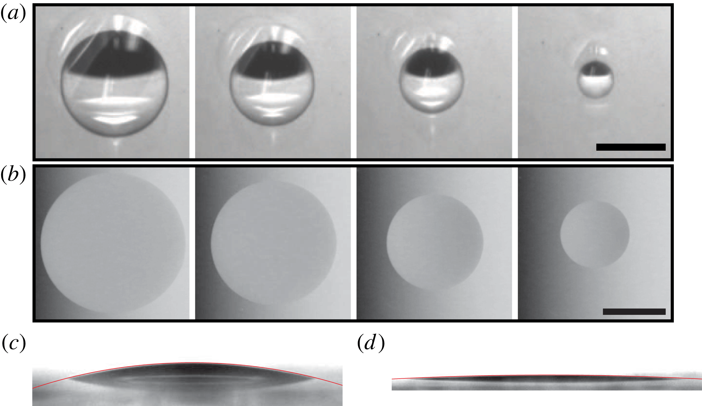
a,b). The perfectly circular drop shape indicates that contact line pinning is not important. Our drops are sufficiently small, so that convection in the gas phase is negligible, and the evaporation rate is limited by vapour diffusion into the surrounding gas phase. Moreover, our drops are very thin, which limits temperature gradients, especially for alkanes that do not evaporate too fast.
Top (a,b) and side (c,d) view of evaporating and spreading drops on clean glass surfaces. (a) Pentane drop, scale bar 5 mm,
 $\text{d}t=6~\text{s}$
. (b) Heptane drop, scale bar 2 mm,
 $\text{d}t=10~\text{s}$
. (c) Peptane drop,
 $R=1.4~\text{mm}$
. (d) Heptane drop,
 $R=2.6~\text{mm}$
, the images include the drop’s reflection on the solid surface, the red line is a spherical cap fit.

Previous studies have found that the contact angle of such a completely wetting but evaporating drop can be non-zero (Bourges-Monnier & Shanahan Reference Bourges-Monnier and Shanahan1995; Cachile et al.
Reference Cachile, Bénichou and Cazabat2002a
,Reference Cachile, Bénichou, Poulard and Cazabat
b
; Poulard et al.
Reference Poulard, Guéna, Cazabat, Boudaoud and Ben Amar2005; Shahidzadeh-Bonn et al.
Reference Shahidzadeh-Bonn, Rafai, Azouni and Bonn2006; Lee et al.
Reference Lee, Cheah, Copleston, Starov and Sefiane2008). The interpretation of such a non-zero contact angle for a completely wetting liquid, which we denote by
 $\unicode[STIX]{x1D703}_{ev}$
, is difficult, since it represents a fundamentally non-equilibrium situation. The presence of stress and evaporative singularities at the contact line, which need to be regularised on a microscopic scale, make the problem inherently multi-scale. A crude regularisation as proposed by Poulard et al. (Reference Poulard, Guéna, Cazabat, Boudaoud and Ben Amar2005) allows us to understand the formation of such an angle but its exact expression has remained a subject of debate (Eggers & Pismen Reference Eggers and Pismen2010; Morris Reference Morris2014). The recent paper by Saxton et al. (Reference Saxton, Whiteley, Vella and Oliver2016) only considers partially wetting liquids (while ignoring pinning of the contact line). The time dependence of the drop radius is also intriguing. Since the fluid is wetting it starts to spread, but at some point, the evaporation starts to dominate, the drop retracts and
 $R$
eventually vanishes at a time
 $t_{0}$
.
In this article, using the framework proposed by Eggers & Pismen (Reference Eggers and Pismen2010), later developed by Morris (Reference Morris2014) we propose a simple parameter free model to describe the spreading dynamics and contact angle of evaporating drops of completely wetting liquids and make a direct comparison with experiments.
2 Experimental set-up
Experiments were performed at room temperature
 $T\approx 21\,^{\circ }\text{C}$
by gently depositing a drop on a float glass surface using a microsyringe, and recording either its weight or shape using a precision balance and a drop shape analyser (Kruss Easydrop, see figure 1
c,d). The alkanes used were ultra pure, from Sigma-Aldrich, the substrate were glass microscope slides (Menzel Gläser, 1 mm thick), cleaned with either sulfochromic acid or piranha solution. The experiments were repeated between 4 and 9 times for each alkane and found to be reproducible to within the error bars presented here. The equilibrium vapour pressure
 $P_{sat}$
of the different alkanes varies over two orders of magnitude, while keeping almost the same density
 $\unicode[STIX]{x1D70C}$
, surface tension
 $\unicode[STIX]{x1D6FE}$
and viscosity
 $\unicode[STIX]{x1D702}$
. The volume of the drops was approximately
 $1~\unicode[STIX]{x03BC}\text{l}$
. The largest radius these drops attained was about 2.5 mm, somewhat larger than the capillary length (1.6–1.8 mm). Although gravity was not completely negligible for these drops, the spherical cap profile remained a good approximation and we used it for simplicity (see appendix A and figure 1
c,d). The drop volume
 $V$
and apparent contact angle
 $\unicode[STIX]{x1D703}$
were then calculated from its measured height
 $h$
and radius
 $R$
. Because some drops are extremely thin, although
 $R$
is measured precisely,
 $h$
is only a few pixels large which results in substantial experimental uncertainties on
 $V$
and
 $\unicode[STIX]{x1D703}$
.
3 Result and discussion
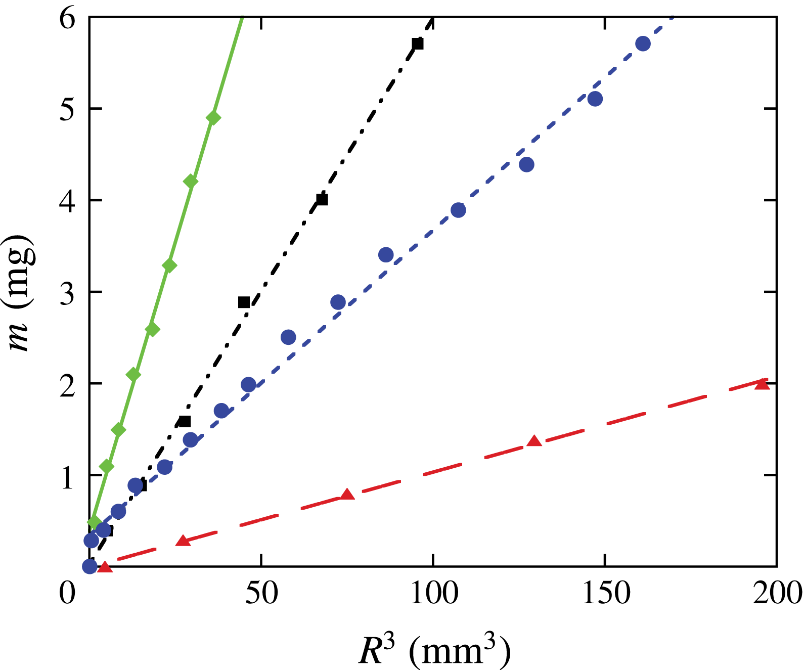
Mass of the drop versus radius cubed; straight lines indicate a constant contact angle. Pentane (C5): green diamonds; hexane (C6): black squares; heptane (C7): blue circles; octane (C8): red triangles.

Figure 2 shows the mass
 $m$
of various alkane drops as a function of their radius cubed as they evaporate, giving a straight line. For a thin drop,
 $\unicode[STIX]{x1D703}=4m/(\unicode[STIX]{x03C0}\unicode[STIX]{x1D70C}R^{3})$
, so that the slope in figure 2 directly corresponds to the contact angle, which is seen to depend strongly on the chain length of the alkane, despite their similar interfacial properties. The macroscopic contact angle is thus controlled by evaporation rather than the wetting properties; due to their low surface tension in equilibrium the contact angle of all alkanes on the substrate is zero.
Turning to the drop dynamics, the simplest assumption is that to leading order the drop dynamics is unaffected by evaporation, which enters through the total mass balance only. Thus drop motion is described by Tanner’s law (Bonn et al.
Reference Bonn, Eggers, Indekeu, Meunier and Rolley2009):
 $R\sim V^{3/10}(\unicode[STIX]{x1D6FE}t/\unicode[STIX]{x1D702})^{1/10}$
, but the total mass flux is proportional to the drop radius (Deegan et al.
Reference Deegan, Bakajin, Dupont, Huber, Nagel and Witten2000):
 $$\begin{eqnarray}\dot{V}=-4\unicode[STIX]{x1D6FD}R,\end{eqnarray}$$
with
 $\unicode[STIX]{x1D6FD}$
the evaporation parameter. Solving the resulting differential equation for
 $V$
, and substituting back into Tanner’s law to find
 $R$
, we find
 $$\begin{eqnarray}R\propto [t_{0}^{11/10}-t^{11/10}]^{3/7}t^{1/10}.\end{eqnarray}$$
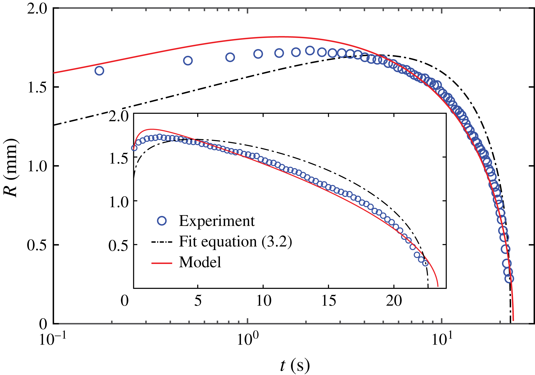
Figure 3 shows (3.2) as the dot-dashed line, with both a prefactor and
 $t_{0}$
as adjustable parameters. Clearly, this simple theory is unable to describe the drop dynamics satisfactorily, demonstrating that evaporation must be included into the description of the contact line dynamics itself, rather than including it phenomenologically.
Spreading and evaporation of a
 $0.32~\unicode[STIX]{x03BC}\text{l}$
heptane drop with a best fit of (3.2) as the dot-dashed line (prefactor
 $=$
0.36,
 $t_{0}=22.6$
), and our model as the red solid curve. Inset: same data on a linear scale.

To do better, one needs to solve the viscous flow problem in the drop coupled to the evaporation which is limited by the diffusion of the vapour. For thin isothermal drops, the flow is simplified through the lubrication approximation and the flow profile is parabolic. The evolution of the drop shape is given by mass conservation (in axisymmetric coordinates),
 $$\begin{eqnarray}\frac{\unicode[STIX]{x2202}h}{\unicode[STIX]{x2202}t}+\frac{1}{r}\frac{\unicode[STIX]{x2202}}{\unicode[STIX]{x2202}r}\left(\frac{h^{3}r}{3\unicode[STIX]{x1D702}}\frac{\unicode[STIX]{x2202}p}{\unicode[STIX]{x2202}r}\right)=-j_{ev},\quad j_{ev}=-\frac{D}{\unicode[STIX]{x1D70C}}\frac{\unicode[STIX]{x2202}\unicode[STIX]{x1D70C}_{v}}{\unicode[STIX]{x2202}z},\end{eqnarray}$$
 $p$
is the pressure driving the flow and
 $j_{ev}$
the local volume flux induced by the diffusion limited evaporation (
 $\unicode[STIX]{x1D70C}_{v}$
is the vapour density and
 $D$
is the diffusion coefficient of the vapour in air).
At the macroscopic scale, the pressure is simply the Laplace pressure and the vapour concentration is given by Laplace’s equation
 $\unicode[STIX]{x1D6FB}^{2}\unicode[STIX]{x1D70C}_{v}=0$
with boundary condition
 $\unicode[STIX]{x1D70C}_{v}=\unicode[STIX]{x1D70C}_{sat}$
, the saturation vapour density at the drop surface and
 $\unicode[STIX]{x1D70C}_{v}=\unicode[STIX]{x1D70C}_{\infty }$
far from the drop (
 $\unicode[STIX]{x1D70C}_{\infty }=0$
for alkanes). Approximating the thin drop as a disc allows us to compute the vapour field
 $\unicode[STIX]{x1D70C}_{v}$
, the volume flux
 $j_{ev}=2\unicode[STIX]{x1D6FD}/(\unicode[STIX]{x03C0}\sqrt{R^{2}-r^{2}})$
(Jackson Reference Jackson1975) and the evaporation parameter
 $\unicode[STIX]{x1D6FD}=D(\unicode[STIX]{x1D70C}_{sat}-\unicode[STIX]{x1D70C}_{\infty })/\unicode[STIX]{x1D70C}$
(Cazabat & Guena Reference Cazabat and Guena2010). However, this macroscopic description suffers from the usual viscous stress divergence at the contact line, also present without evaporation (Bonn et al.
Reference Bonn, Eggers, Indekeu, Meunier and Rolley2009; Eggers & Fontelos Reference Eggers and Fontelos2015). In addition,
 $j_{ev}$
is also singular at
 $r=R$
(the divergence persists for spherical caps with low contact angle (Deegan et al.
Reference Deegan, Bakajin, Dupont, Huber, Nagel and Witten2000)). To deal with the problem one has to introduce microscopic effects to regularise the singularities.
A first attempt was made by Poulard et al. (Reference Poulard, Guéna, Cazabat, Boudaoud and Ben Amar2005) using scaling arguments. They introduce the distance from the contact line where van der Waals forces balance capillary forces and assume that the evaporation rate saturates below this scale. The resulting model being based on scaling arguments, Poulard et al. (Reference Poulard, Guéna, Cazabat, Boudaoud and Ben Amar2005) did not perform a direct comparison with experiments. Nonetheless, their model predicts power laws for
 $R(t)$
during the retraction stage that agree with the ones observed experimentally.
More recently, Eggers & Pismen (Reference Eggers and Pismen2010) introduced van der Waals forces self-consistently in the coupled problem through a disjoining pressure term
 $\unicode[STIX]{x1D6F1}=A/(6\unicode[STIX]{x03C0}h^{3})=\unicode[STIX]{x1D6FE}a^{2}/h^{3}$
(
 $A$
is the Hamaker constant, and
 $a$
is a microscopic length). A consequence is that far from the drop, (attractive) van der Waals interactions compete with evaporation to condensate a microscopic prewetting film whose thickness
 $h_{f}$
is given by a balance of evaporative to disjoining pressure
 $h_{f}^{3}=\unicode[STIX]{x1D6FE}a^{2}/(\unicode[STIX]{x1D70C}R_{s}T\ln (\unicode[STIX]{x1D70C}_{\infty }/\unicode[STIX]{x1D70C}_{sat}))$
with
 $R_{s}$
the specific gas constant. In addition, Eggers & Pismen (Reference Eggers and Pismen2010) included the Kelvin effect which takes the local curvature of the drop into account. They showed that taking these effects into account regularises the evaporative singularity as it inhibits evaporation. Equation (3.3) then becomes:
 $$\begin{eqnarray}\left.\begin{array}{@{}c@{}}{\displaystyle \frac{\unicode[STIX]{x2202}h}{\unicode[STIX]{x2202}t}}+{\displaystyle \frac{\unicode[STIX]{x1D6FE}}{\unicode[STIX]{x1D702}r}}{\displaystyle \frac{\unicode[STIX]{x2202}}{\unicode[STIX]{x2202}r}}\left[{\displaystyle \frac{h^{3}r}{3}}{\displaystyle \frac{\unicode[STIX]{x2202}}{\unicode[STIX]{x2202}r}}\left({\displaystyle \frac{\unicode[STIX]{x2202}^{2}h}{\unicode[STIX]{x2202}r^{2}}}+{\displaystyle \frac{1}{r}}{\displaystyle \frac{\unicode[STIX]{x2202}h}{\unicode[STIX]{x2202}r}}+{\displaystyle \frac{a^{2}}{h^{3}}}\right)\right]=-j_{ev},\\ j_{ev}={\displaystyle \frac{\unicode[STIX]{x1D6FD}}{r}}{\displaystyle \frac{\unicode[STIX]{x2202}}{\unicode[STIX]{x2202}r}}\left[\displaystyle \int _{0}^{\infty }{\mathcal{K}}(r,r^{\prime }){\displaystyle \frac{\unicode[STIX]{x2202}}{\unicode[STIX]{x2202}r^{\prime }}}\left({\displaystyle \frac{h_{f}}{h}}\right)^{3}\,\text{d}r^{\prime }\right].\end{array}\right\}\end{eqnarray}$$
The kernel is given by
 $$\begin{eqnarray}{\mathcal{K}}(r,r^{\prime })=\frac{2}{\unicode[STIX]{x03C0}}\left\{\begin{array}{@{}ll@{}}r[\mathit{K}(r^{\prime }/r)-\mathit{E}(r^{\prime }/r)],\quad & r^{\prime }<r\\ r^{\prime }[\mathit{K}(r/r^{\prime })-\mathit{E}(r/r^{\prime })],\quad & r^{\prime }>r,\end{array}\right.\end{eqnarray}$$
where
 $\mathit{K}$
and
 $\mathit{E}$
are the complete elliptic integrals.
In the quasi-static limit, which means that when considering evaporation, the time derivative in (3.4) is neglected, Morris (Reference Morris2014) shows that the contact region can be described analytically in the case of vanishing
 $\mathscr{L}$
. This allows for the exact computation of the cutoff length introduced by hand by Poulard et al. (Reference Poulard, Guéna, Cazabat, Boudaoud and Ben Amar2005) and the determination of the evaporative angle (Morris Reference Morris2014, see appendix B for the derivation of the closed form solution presented below). The result is
 $$\begin{eqnarray}\unicode[STIX]{x1D703}_{ev}=k\left(\frac{\unicode[STIX]{x1D702}\unicode[STIX]{x1D6FD}}{\unicode[STIX]{x1D6FE}a^{1/2}R^{1/2}}\right)^{1/3},\end{eqnarray}$$
where
 $k$
can be assumed constant and is given by
 $$\begin{eqnarray}\left.\begin{array}{@{}c@{}}k=1.47758{\displaystyle \frac{2^{1/6}}{\unicode[STIX]{x03C0}^{1/3}}}\mathit{W}\left({\displaystyle \frac{4}{\mathscr{L}^{3/2}}}\right)^{1/6},\\ \mathscr{L}={\displaystyle \frac{2^{2/3}\unicode[STIX]{x1D70C}_{sat}^{4/3}(\unicode[STIX]{x1D702}\unicode[STIX]{x1D6FD})^{16/9}}{\unicode[STIX]{x03C0}^{4/9}a^{26/9}R^{2/9}\unicode[STIX]{x1D6FE}^{4/9}(R_{s}T\unicode[STIX]{x1D70C}\left(\unicode[STIX]{x1D70C}_{sat}-\unicode[STIX]{x1D70C}_{\infty }\right))^{4/3}}},\end{array}\right\}\end{eqnarray}$$
were
 $\mathit{W}$
denotes the Lambert
 $W$
function (see appendix B and table 2 for values of
 $\mathscr{L}$
and
 $k$
).
Motion is such that the apparent contact angle
 $\unicode[STIX]{x1D703}$
is driven toward
 $\unicode[STIX]{x1D703}_{ev}$
according to the Cox–Voinov law (Eggers & Fontelos Reference Eggers and Fontelos2015):
 $$\begin{eqnarray}{\dot{R}}=\frac{\unicode[STIX]{x1D6FE}}{9B\unicode[STIX]{x1D702}}\left[\left(\frac{4V}{\unicode[STIX]{x03C0}R^{3}}\right)^{3}-\unicode[STIX]{x1D703}_{ev}^{3}\right],\end{eqnarray}$$
where
 $B$
is the usual logarithmic molecular cutoff also present without evaporation (see appendix B).
Equations (3.1), (3.6), (3.8) derived here are the same as the scaling analysis proposed in Poulard et al. (Reference Poulard, Guéna, Cazabat, Boudaoud and Ben Amar2005); however, because of the nature of their analysis, they were unable to calculate the prefactors and the discussion remained qualitative. Here we have done the full analysis; the evaporative cutoff is calculated by including the effect of disjoining pressure self-consistently (Morris Reference Morris2014).
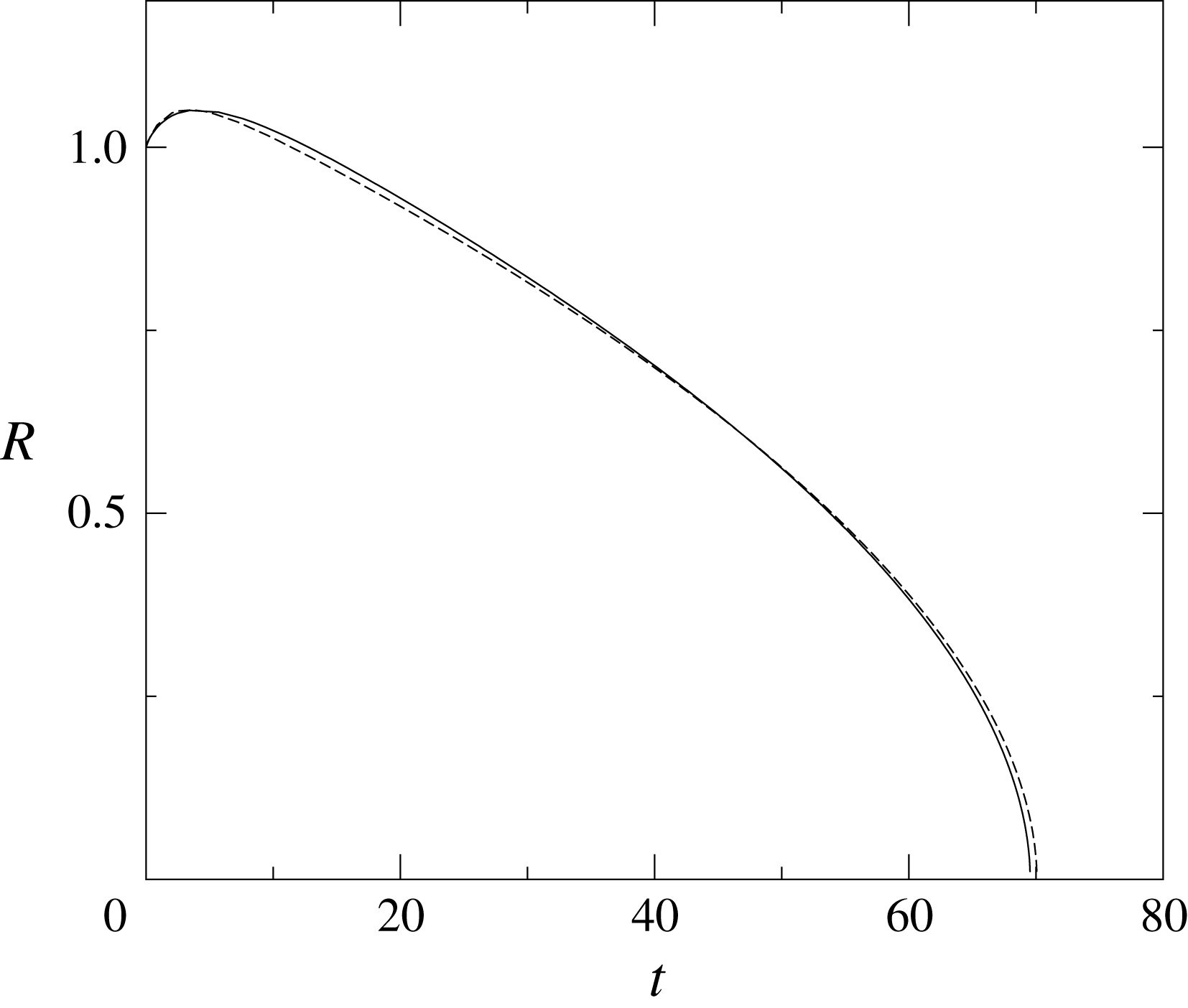
We have simulated the complete equations of motion (3.4), (3.5) with parameters that lie in the quasi-static regime and compared it to the model (3.1), (3.6), (3.8) in figure 4 (lengths are rescaled with the initial drop radius
 $R_{0}$
and time with
 $R_{0}\unicode[STIX]{x1D702}/\unicode[STIX]{x1D6FE}$
). The model shows a very good agreement with the simulation with a fitted value
 $k_{\mathit{fit}}=1.9$
close to the one predicted by (3.7)
 $k=1.69$
(see appendix B).
Dimensionless radius as a function of the dimensionless time for an evaporating drop, with
 $V_{0}=1$
,
 $\unicode[STIX]{x1D6FD}=5\times 10^{-3}$
,
 $a=10^{-3}$
and
 $h_{f}=10^{-4}$
. The solid line is the simulation and the dashed line is theory with
 $k$
fitted to
 $k_{\mathit{fit}}=1.9$
, a value close to the one predicted by the model
 $k=1.69$
(
 $B\approx 2.1$
with these parameters).

Now, comparing the model to experimental data, we first measure the evaporation parameter
 $\unicode[STIX]{x1D6FD}$
independently by fitting (3.1) to the data.
 $\dot{V}$
being noisy for very thin droplets, the uncertainty on
 $\unicode[STIX]{x1D6FD}$
is substantial and we adjust the value used in the model within this uncertainty. We then estimate
 $a\approx 4~\mathring{A}$
using Lifshitz theory (Israelachvili Reference Israelachvili2011),
 $B$
in (3.8) is calculated from (B 6) and varies between 5.38 and 6.03 (table 2). The range being narrow we use the mean value 5.6 for all our experimental comparisons. Similarly we calculate the parameter
 $k$
in (3.6) from (3.7). It varies between 1.42 and 1.69 (table 2) and we use an intermediate value of 1.62 for all our experiments.
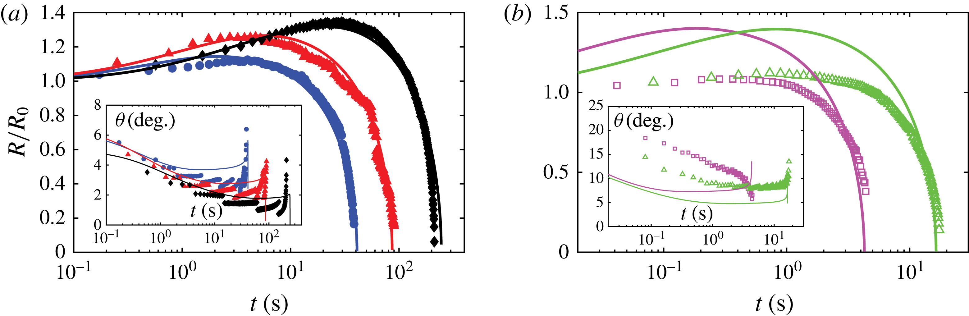
Figures 3 and 5 compare
 $R(t)$
from the model with the experimental data for various alkanes. We find excellent agreement for slowly evaporating alkanes: heptane to nonane, without any free parameters, cf. figure 5(a). In addition, within the experimental accuracy, the macroscopic contact angle
 $\unicode[STIX]{x1D703}(t)$
is also well described by these equations, and approaches a constant steady-state value at late times (inset figure 5
a). For pentane and hexane, for which evaporation is very rapid, the drop hardly spreads and the contact line recedes quickly (figure 5
b). During the short spreading time,
 $\unicode[STIX]{x1D703}$
decreases significantly (inset of figure 5
b); this means that
 $\unicode[STIX]{x2202}h/\unicode[STIX]{x2202}t$
is not small, and the quasi-static assumption used in the model is not valid. Moreover, the cooling due to evaporation increases with the evaporation rate
 $\unicode[STIX]{x1D6FD}$
and neglecting the temperature gradient and resulting Marangoni flows becomes incorrect (see appendix A for a critical discussion of the model’s assumptions). As a result, the model is only able to reproduce this dynamics qualitatively, as it overestimates the spreading motion at short times.
Dimensionless radius of spreading and evaporating alkane drops. Inset: measured contact angle for the same data set, the uncertainties are not reported here for clarity (see figure 6). (a) Blue circles: heptane; red triangles: octane; black diamonds: nonane. (b) Pink open squares: pentane; green open triangles: hexane.

As for the contact angle, the breakdown of the quasi-static and isothermal assumptions means that the measured angle does not necessarily converge to
 $\unicode[STIX]{x1D703}_{ev}$
given by (3.6). Nevertheless, the experimental contact angle
 $\unicode[STIX]{x1D703}$
reaches a steady-state value close to
 $\unicode[STIX]{x1D703}_{ev}$
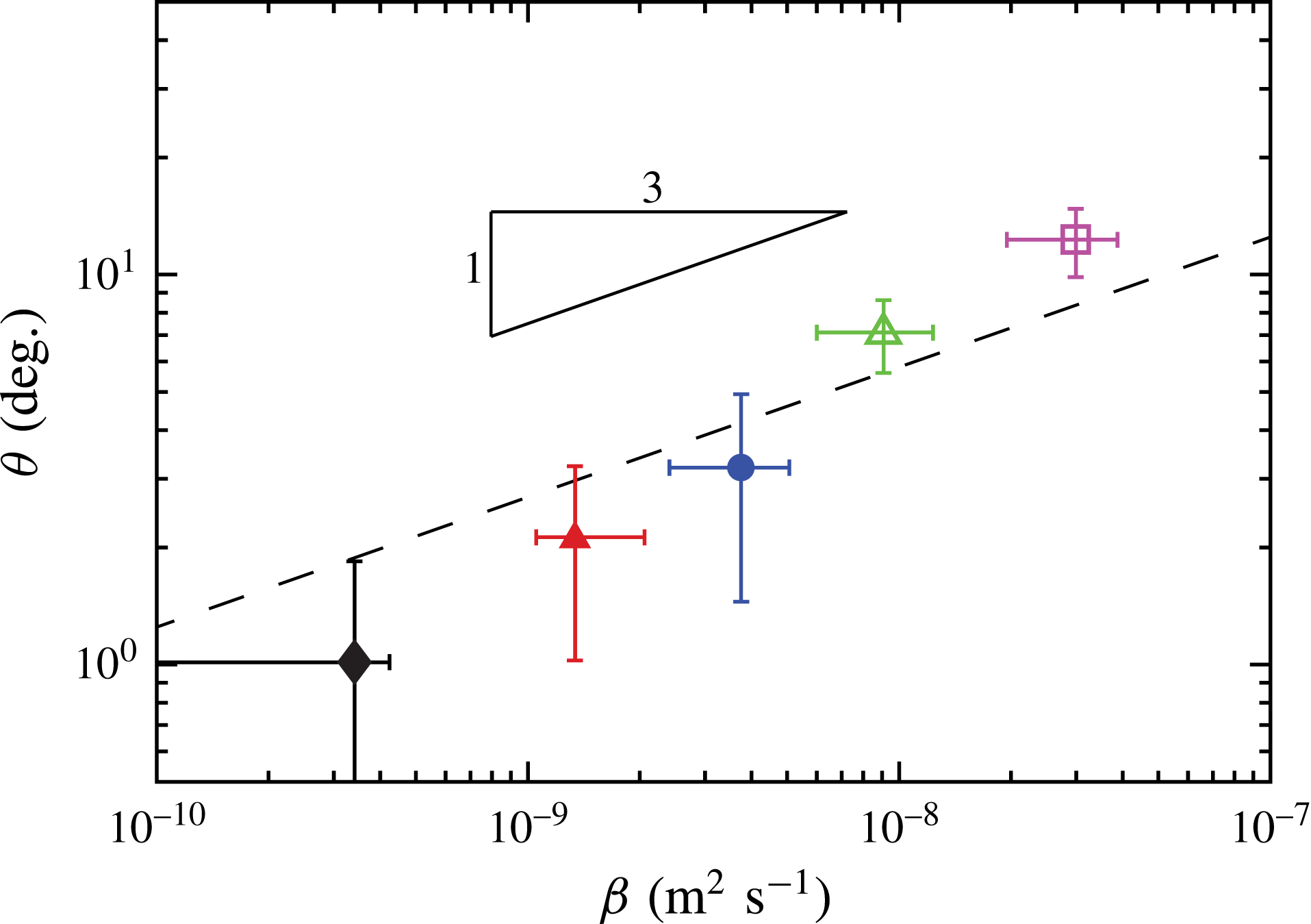
. We plot this value as a function of
 $\unicode[STIX]{x1D6FD}$
for the different alkanes in figure 6. Within the experimental uncertainties (that become significant when the drop is very thin) one retrieves the
 $1/3$
rd power law predicted by (3.6) with the correct prefactor.
Contact angle at late times
 $\unicode[STIX]{x1D703}$
as a function of the evaporation parameter
 $\unicode[STIX]{x1D6FD}$
. The dashed line is equation (3.6), neglecting the small variations in the parameters for alkanes:
 $\unicode[STIX]{x1D703}_{ev}(\mathit{rad})=46.88\unicode[STIX]{x1D6FD}^{1/3}$
.

4 Conclusion
In summary, we studied the dynamics of perfectly wetting, volatile fluids on a solid substrate for a wide range of evaporation rates. Taking into account the spreading dynamics and using a consistent description of evaporation near the contact line, we were able to obtain a quantitative agreement between our parameter free model and experiments during both spreading and retraction phases for slowly evaporating alkanes. For very volatile liquids, the agreement is only qualitative as temperature gradients and dynamic effects, neglected in the model, become significant.
Acknowledgement
This work received a financial grant from the ‘French Agence Nationale de la Recherche’; project ANR-13-BS09-0026.
Appendix A.
We make a number of approximations in our model to keep it tractable: we assume gravity and inertia to be negligible, the system to be isothermal (and thus without any Marangoni flows), the drop movement to be quasi-static and the transport of vapour to be purely diffusive (neglecting convection and kinetic effects). We will now discuss the validity of these assumptions using the dimensionless groups as proposed in Larson (Reference Larson2014).
A.1 Diffusive vapour transport
Because the experiments are carried out in a box to limit air flows around the drop, the only source of convection in our experiment is the natural convection due to the buoyancy of the alkane vapour in the air. The Grashof number
 $Gr$
, which balances buoyancy with viscous forces, controls the strength of this natural convection. Assuming the gas to be ideal and the vapour concentration to be the saturation concentration, we have
 $$\begin{eqnarray}Gr=\frac{(\unicode[STIX]{x1D70C}_{sat}-\unicode[STIX]{x1D70C}_{\infty })gR^{3}}{\unicode[STIX]{x1D70C}_{air}\unicode[STIX]{x1D708}_{air}^{2}},\end{eqnarray}$$
where
 $\unicode[STIX]{x1D70C}_{air}$
is the air density and
 $\unicode[STIX]{x1D708}_{air}$
the air kinematic viscosity.
Kelly-Zion et al. (Reference Kelly-Zion, Pursell, Vaidya and Batra2011) studied the effect of natural convection in evaporating sessile drops with pinned contact line. They found the empirical relationship
 $$\begin{eqnarray}\dot{V}=-4\unicode[STIX]{x1D6FD}R(1+0.310Gr^{0.216}),\end{eqnarray}$$
which differs significantly from the purely diffusive case if
 $0.310Gr^{0.216}>1$
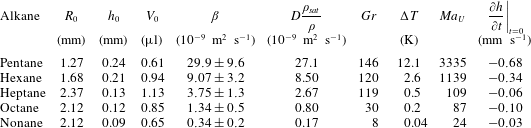
. We show in table 1 the Grashof number corresponding to our experiments (using
 $R_{0}$
for the drop radius). According to Kelly-Zion et al. (Reference Kelly-Zion, Pursell, Vaidya and Batra2011), the maximum convective contribution we can expect (as
 $R$
decreases after the spreading phase) ranges between 0.5 and 0.9 times the diffusive contribution, which is neither dominant nor negligible. Nonetheless our
 $\dot{V}=f(R)$
data are fairly linear, but with a coefficient
 $\unicode[STIX]{x1D6FD}$
somewhat higher than
 $D\unicode[STIX]{x1D70C}_{sat}/\unicode[STIX]{x1D70C}$
, the value expected in the purely diffusive case (see table 1,
 $\unicode[STIX]{x1D70C}_{\infty }=0$
for alkanes). Although this is difficult to quantify given our experimental uncertainties, there might be a little bit of convection in some of our experiments. Though this is not the reason why the model fails to describe the dynamics for short alkanes. For hexane and pentane the discrepancies are small and replacing (3.1) by (A 2) does not improve the model significantly. Thus we keep the pure diffusion approximation in our model, but we use the measured
 $\unicode[STIX]{x1D6FD}$
directly instead of using the predicted value
 $D\unicode[STIX]{x1D70C}_{sat}/\unicode[STIX]{x1D70C}$
.
Parameters used to assess the validity of our assumptions; the experimental values corresponds to the experiment presented in figure 5,
 $D$
values at
 $T=22^{\circ }$
come from Berezhnoi & Semenov (Reference Berezhnoi and Semenov1997), Beverley, Clint & Fletcher (Reference Beverley, Clint and Fletcher1999),
 $P_{sat}$
values from Carruth & Kobayashi (Reference Carruth and Kobayashi1973) and Beverley et al. (Reference Beverley, Clint and Fletcher1999).

If the diffusion of the vapour in the ambient gas is very fast, for instance under reduced pressure or if the ambient gas is pure vapour, then the evaporation can become affected by kinetic effects: the transfer of molecules from the liquid to the vapour at the interface (given by the Hertz–Knudsen relation). This effect reduces the concentration of vapour at the liquid–vapour interface and thus the overall evaporation rate. However, scaling arguments (Cazabat & Guena Reference Cazabat and Guena2010; Larson Reference Larson2014) and numerical simulations (Semenov et al. Reference Semenov, Starov, Rubio and Velarde2012) have shown that this effect is negligible for common liquids in ambient air, except for microscopic droplets. Moreover, pure diffusion predicts our measured evaporation rate satisfactorily so we neglect interfacial kinetic effects.
A.2 Temperature effects
The possible temperature gradients in the drop come from the heat loss due to latent heat of evaporation whose average rate is
 $\unicode[STIX]{x1D70C}\dot{V}\unicode[STIX]{x0394}H_{vap}/\unicode[STIX]{x03C0}R^{2}$
, with
 $\unicode[STIX]{x0394}H_{vap}$
the heat of vaporisation per unit mass. This flux must be balanced by steady-state heat conduction from the substrate of the order of
 $k_{l}\unicode[STIX]{x0394}T/h$
with
 $k_{l}$
the liquid thermal conductivity. Equating the two allows us to evaluate the temperature difference between the top and bottom of the drop:
 $$\begin{eqnarray}\unicode[STIX]{x0394}T\sim \frac{4\unicode[STIX]{x1D70C}\unicode[STIX]{x1D6FD}\unicode[STIX]{x0394}H_{vap}h}{\unicode[STIX]{x03C0}k_{l}R}.\end{eqnarray}$$
For alkanes
 $\unicode[STIX]{x0394}H_{vap}\approx 3.5\times 10^{5}~\text{J}~\text{kg}^{-1}$
and
 $k_{l}\approx 0.13~\text{W}~\text{m}^{-1}~\text{K}^{-1}$
,
 $\unicode[STIX]{x0394}T$
is thus directly proportional to
 $\unicode[STIX]{x1D6FD}$
times the drop aspect ratio
 $h/R$
. As the drop aspect ratio is larger for drops which evaporates faster, we immediately see they have the largest temperature gradient.
This simple estimate assumes good substrate conduction relative to the droplet. Although
 $k_{l}$
is ten times smaller than the glass thermal conductivity, because our substrates are quite thick compared to our drops (1 mm) their effect on the temperature field might not be completely negligible. Moreover, our drops have low contact angles such that the evaporation rate (and thus local heat loss) is much stronger at their edge. Equation (A 3) is thus only a rough estimate as both of these effect generates much more complex temperature fields and can even reverse the temperature gradient (Dunn et al.
Reference Dunn, Wilson, Duffy and Sefiane2009; Larson Reference Larson2014).
These temperature gradients induce a Marangoni flow (and to a lesser extent buoyancy-driven flows) whose speed is of the order of
 $-(\text{d}\unicode[STIX]{x1D6FE}/\text{d}T)\unicode[STIX]{x0394}Th/(R\unicode[STIX]{x1D702})$
. The ratio of this speed to the mean speed from evaporation
 $R/t_{0}$
defines an alternative Marangoni number
 $$\begin{eqnarray}Ma_{U}=-\frac{\text{d}\unicode[STIX]{x1D6FE}}{\text{d}T}\frac{\unicode[STIX]{x0394}Tht_{0}}{\unicode[STIX]{x1D702}R^{2}}.\end{eqnarray}$$
We evaluate both
 $\unicode[STIX]{x0394}T$
and
 $Ma_{U}$
for our drops in table 1 using the initial values
 $h_{0}$
,
 $R_{0}$
for the drop shape and our measured value of
 $\unicode[STIX]{x1D6FD}$
(for alkanes
 $\text{d}\unicode[STIX]{x1D6FE}/\text{d}T\approx -10^{-4}~\text{N}~\text{m}^{-1}$
). The temperature difference is very large for pentane drops, still significant for hexane drops and much lower for the other alkanes. The Marangoni numbers is thus much higher for pentane and hexane. As pointed by Larson (Reference Larson2014), even with good substrate conduction and hemispherical drops this analysis is qualitative, for instance the full numerical analysis in Savino & Fico (Reference Savino and Fico2004) gives values 30 times lower. So even though
 $Ma_{U}>1$
for heptane, octane and nonane drops, the good agreement with our theory suggests negligible Marangoni flows. Indeed, with the additional effects due to the substrate and low contact angle, a factor 100 between our crude assumption and reality is plausible. For pentane and hexane drops however, the Marangoni flows are probably dominant. Computing the usual Marangoni number
 $Ma=Ma_{U}(R^{2}/\unicode[STIX]{x1D6FC}_{l}t_{0})$
, with
 $\unicode[STIX]{x1D6FC}_{l}\sim 10^{-7}~\text{m}^{2}~\text{s}^{-1}$
the thermal diffusivity, yields similar results;
 $Ma\sim 10^{3}{-}10^{4}$
for pentane and hexane, well above the planar Bénard–Marangoni instability threshold (
 $Ma_{c}\sim 10^{2}$
) which suggests convection rolls in the drop.
Thus our neglect of the Marangoni stress in the lubrication analysis partly explains the discrepancy between model and experiment for the spreading dynamics and evaporative angle.
A.3 Quasi-steadiness
To evaluate the quasi-static assumption we calculate characteristic time scales of our drops and compare them to the evaporation duration
 $t_{0}$
. The characteristic time for heat equilibration inside the drop is
 $t_{heat}\sim h_{0}^{2}/\unicode[STIX]{x1D6FC}_{l}$
. Because the initial drop height
 $h_{0}$
decreases with the chain length (see table 1), so does
 $t_{heat}$
, which varies between
 $0.08\lesssim t_{heat}~(\text{s})\lesssim 0.5$
. The drying time
 $t_{0}$
, however increases with the chain length
 $5\lesssim t_{0}~(\text{s})\lesssim 200$
. Since
 $t_{0}\gg t_{heat}$
, we can neglect the time dependence of the temperature in the drop. Similarly the characteristic time for the velocity inside the drop to reach a steady state is
 $t_{mom}\sim h_{0}^{2}\unicode[STIX]{x1D70C}/\unicode[STIX]{x1D702}$
. It also decreases with the chain length of the alkane and varies between
 $0.01\lesssim t_{mom}~(\text{s})\lesssim 0.15$
. Again, since the drying time
 $t_{0}$
is much larger, the quasi-static approach is in general valid. However, the most unfavourable cases are pentane and hexane. For these fast evaporating alkane the spreading motion is very fast, and the reversal of the contact line occurs at
 $t_{R_{max}}\sim 0.5~\text{s}$
. During the spreading motion the system has not yet had time to reach a steady state. If we evaluate
 $\unicode[STIX]{x2202}h/\unicode[STIX]{x2202}t$
experimentally from the first two recorded frames (when the drop is completely detached from the pipette) we find a significantly higher value for pentane and hexane (see table 1) which consequently may not be negligible.
A.4 Inertia and gravity
Because ours drops are very thin, we use the lubrication approximation which neglects inertia. The lubrication approximation is valid when the Reynolds number is much smaller than the (large) aspect ratio, i.e. when
 $\unicode[STIX]{x1D70C}{\dot{R}}h^{2}/(\unicode[STIX]{x1D702}R)\ll 1$
. For all our drops this is verified as
 $10^{-7}<\unicode[STIX]{x1D70C}{\dot{R}}h^{2}/(\unicode[STIX]{x1D702}R)<10^{-1}$
, the worst case being the initial fast spreading of pentane.
The volume of our drops is very small (
 ${\sim}1~\unicode[STIX]{x03BC}\text{l}$
); however because they are very thin they can have radii of the order of the capillary length
 $\ell _{c}=\sqrt{\unicode[STIX]{x1D6FE}/(\unicode[STIX]{x1D70C}g)}$
so that it is not very clear whether gravity is completely negligible. To test for its influence, we compared the spherical cap profile to the numerical solution of the Young–Laplace equation. For our pentane and hexane drops, there is no appreciable difference, while for heptane, octane and nonane there is a subtle flattening which is however too small to be detected experimentally, explaining the good spherical cap fit seen in figure 1(d). To check if this small difference impairs our measurement, we have compared the contact angles and volumes obtained with the spherical cap assumption to the one obtained with the small slope approximation of the Young–Laplace equation (Allen Reference Allen2003)
 $$\begin{eqnarray}\unicode[STIX]{x1D703}_{ss}=\frac{h}{R}\frac{Bo\text{I}_{1}(Bo)}{\text{I}_{0}(Bo)-1}=\frac{V}{\unicode[STIX]{x03C0}R^{3}}\frac{Bo^{2}\text{I}_{1}(Bo)}{Bo\text{I}_{0}(Bo)-2\text{I}_{1}(Bo)},\end{eqnarray}$$
where
 $Bo=R/\ell _{c}$
and
 $\text{I}_{n}$
represent the modified Bessel function of the first kind. For pentane and hexane the two methods provided the same results, while for heptane, octane and nonane
 $\unicode[STIX]{x1D703}$
is approximately 10 % higher with the small slope approximation. These differences are quite small, much smaller than the experimental uncertainties, thus confirming that the spherical cap assumption is a good approximation for our drops.
For even larger drops our model could be adapted to include gravity. The evaporative flux (eventually modified to include buoyant convection) and the Cox–Voinov law are still valid in the gravity dominated regime, although with an adjusted prefactor
 $B$
(Alizadeh Pahlavan et al.
Reference Alizadeh Pahlavan, Cueto-Felgueroso, McKinley and Juanes2015). One could thus use (3.1), (3.8) with the apparent angle term
 $4V/(\unicode[STIX]{x03C0}R^{3})$
replaced by (A 5). The corner analysis done by Morris (Reference Morris2014) to derive the evaporative angle would also still be mostly valid, one just needs to change the asymptotic matching condition with the main drop to get the evaporative angle for pancakes.
Appendix B.
With a local analysis of the coupled equations (3.4) in the vicinity of the contact line and in the quasi-static limit, Morris (Reference Morris2014) predicted the macroscopic contact angle of the drop
 $\unicode[STIX]{x1D703}_{ev}$
in the asymptotic limit
 $\mathscr{L}\rightarrow 0$
(Morris (Reference Morris2014, equation (6.3))):
 $$\begin{eqnarray}\unicode[STIX]{x1D703}_{ev}=1.47758\left(\frac{2\sqrt{2}}{\unicode[STIX]{x03C0}}\frac{\unicode[STIX]{x1D702}\unicode[STIX]{x1D6FD}}{\unicode[STIX]{x1D6FE}a^{1/2}R^{1/2}}\right)^{1/3}\ell _{1}^{1/4}.\end{eqnarray}$$
Here
 $\mathscr{L}$
is the Laplace parameter, which is a dimensionless surface tension controlling the coupled problem (defined in (3.7)) and
 $\{\ell _{1},h_{1}\}$
are the dimensionless location and height at which the capillary and disjoining pressures balance in the wetting film, respectively. These lengths are given by (see Morris (Reference Morris2014, equation (5.10))):
 $$\begin{eqnarray}\mathscr{L}\ell _{1}h_{1}^{4}=1\quad \text{and}\quad \ell _{1}=\left({\textstyle \frac{3}{2}}\ln h_{1}\right)^{2/3}.\end{eqnarray}$$
Eliminating
 $\ell _{1}$
from (B 2) we arrive at:
 $$\begin{eqnarray}\frac{4}{\mathscr{L}^{3/2}}=\frac{4}{\mathscr{L}^{3/2}h_{1}^{6}}\exp \left(\frac{4}{\mathscr{L}^{3/2}h_{1}^{6}}\right),\end{eqnarray}$$
which can be solved in terms of the Lambert W function, and we obtain:
 $$\begin{eqnarray}h_{1}=\left(\frac{4}{\mathscr{L}^{3/2}\text{W}\left(4/\mathscr{L}^{3/2}\right)}\right)^{1/6},\quad \ell _{1}=\left(\frac{\text{W}(4/\mathscr{L}^{3/2})}{4}\right)^{2/3}.\end{eqnarray}$$
Replacing (B 4) in (B 1), we obtain the final closed form equation for the evaporative contact angle: equation (3.7).
We show in table 2 the values obtained for
 $\mathscr{L}$
and
 $k$
using (3.7) with the measured value of
 $\unicode[STIX]{x1D6FD}$
and
 $R_{0}$
. Since
 $R$
varies during an experiment,
 $\mathscr{L}$
and thus
 $k$
are not strictly constant, yet their variations are small so we neglect them. For instance
 $1.9\times 10^{-3}<\mathscr{L}<3.0\times 10^{-3}$
and
 $1.60<k<1.62$
for the octane drop of figure 5 (the minimum recorded drop radius is 0.3 mm).
 $\mathscr{L}$
ranges between
 $3\times 10^{-4}$
for nonane and
 $8\times 10^{-2}$
for pentane, which gives
 $k\approx 1.55$
(see table 2).
The prefactor
 $k$
for the simulations is also obtained with (3.7) using the corresponding value of
 $\mathscr{L}$
which is computed from the linearised prewetting film thickness
 $h_{f}^{3}=\unicode[STIX]{x1D70C}_{sat}\unicode[STIX]{x1D6FE}a^{2}/(R_{s}T\unicode[STIX]{x1D70C}(\unicode[STIX]{x1D70C}_{sat}-\unicode[STIX]{x1D70C}_{\infty }))$
used in the simulation (Eggers & Pismen Reference Eggers and Pismen2010). Using dimensionless variables (length rescaled with
 $R_{0}$
and time with
 $R_{0}\unicode[STIX]{x1D702}/\unicode[STIX]{x1D6FE}$
) we get:
 $$\begin{eqnarray}\mathscr{L}=\frac{2^{2/3}\unicode[STIX]{x1D6FD}^{16/9}h_{f}^{4}}{\unicode[STIX]{x03C0}^{4/9}a^{50/9}R^{2/9}}.\end{eqnarray}$$
Strictly speaking the linearisation is not correct far from the drop when
 $\unicode[STIX]{x1D70C}_{\infty }=0$
, but still holds locally close to the contact line (Morris Reference Morris2014). The prefactor for figure 4,
 $k=1.69$
is very close to experimental ones shown in table 2 despite the very different values of the parameters.
Equations (3.6) and (3.7) predict the experimental steady-state contact angle quantitatively, except for pentane and hexane (see figure 5
b), for which a discrepancy larger than the uncertainties starts to appear. As discussed above some of the model’s assumption break down for these drops, the isothermal assumption is incorrect and the quasi-static assumption becomes doubtful. We can also notice that
 $\mathscr{L}$
is much larger such that the limit
 $\mathscr{L}\rightarrow 0$
might not be reached.
Parameters deduced from the model for figure 5.

As in all moving contact line problems, the viscous stress in the vicinity of the contact line must be regularised in order to predict the drop radius as a function of time
 $R(t)$
. This is usually done by introducing a cutoff length, which results in a logarithmic prefactor
 $B$
in the equation of motion in the contact line (de Gennes Reference de Gennes1985; Bonn et al.
Reference Bonn, Eggers, Indekeu, Meunier and Rolley2009). In the very beginning of our experiment, spreading is dominant and the drop moves over a prewetting film. We thus use the cutoff length derived for spreading drops without evaporation (Bonn et al.
Reference Bonn, Eggers, Indekeu, Meunier and Rolley2009; Eggers & Fontelos Reference Eggers and Fontelos2015):
 $$\begin{eqnarray}B=\ln \left(\frac{R}{1.38e^{2}a}\left(\frac{\unicode[STIX]{x1D702}{\dot{R}}}{\unicode[STIX]{x1D6FE}}\right)^{2/3}\right)\end{eqnarray}$$
and consider it constant throughout the experiment for simplicity (although it was not derived for an evaporating receding contact line). Table 2 shows the values of
 $B$
we obtain using the initial values of the experimental parameters.