1 Introduction
Ice-covered waterbodies show complex circulation patterns characterised by buoyancy-driven processes during late Winter/early Spring season (Farmer Reference Farmer1975; Forrest et al.
Reference Forrest, Laval, Pieters and Lim2013; Rizk, Kirillin & Leppäranta Reference Rizk, Kirillin and Leppäranta2014; Salonen et al.
Reference Salonen, Pulkkanen, Salmi and Griffiths2014; Kirillin et al.
Reference Kirillin, Forrest, Graves, Fischer, Engelhardt and Laval2015; Bouffard et al.
Reference Bouffard, Zdorovennov, Zdorovennova, Pasche, Wüest and Terzhevik2016; Yang et al.
Reference Yang, Young, Brown and Wells2017). Over this period, the primary forcing mechanism of such systems is the radiative buoyancy flux,
 $\unicode[STIX]{x1D6F7}_{r}$
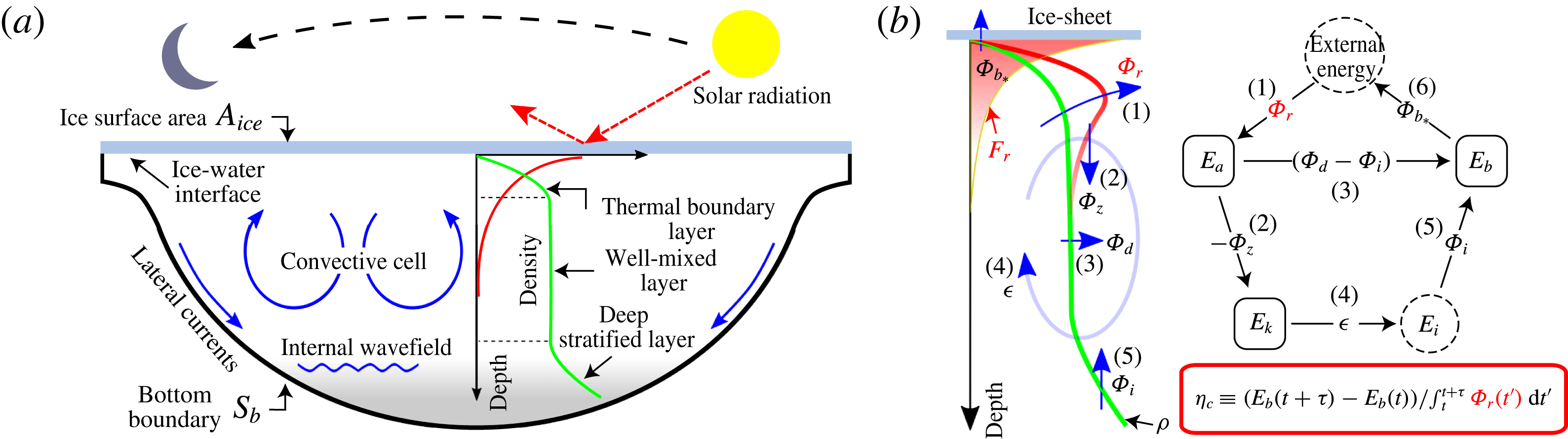
, controlled by solar radiation (daylight) able to penetrate across the ice sheet and heat upper waters. The combination of the radiative heating and the ice boundary on the top of the waterbody imprints a unique signature in the vertical temperature distribution (figure 1
a). The average water temperature profile is characterised by a stable thermal boundary layer (TBL) with temperatures increasing from
 $0\,^{\circ }\text{C}$
at the ice–water interface towards the interior and can extend from tens of centimetres to a couple of metres (Mironov et al.
Reference Mironov, Terzhevik, Kirillin, Jonas, Malm and Farmer2002). The TBL is usually joined to a well-mixed layer, resulting from radiatively driven convection (RDC), and whose thickness can take the remaining water column or end at a depth where deep stratification might be found, with temperatures below or near the maximum water density,
 $T_{md}$
(see figure 1(a) and Farmer Reference Farmer1975; Kirillin et al.
Reference Kirillin, Leppäranta, Terzhevik, Granin, Bernhardt, Engelhardt, Efremova, Golosov, Palshin, Sherstyankin, Zdorovennova and Zdorovennov2012; Bouffard et al.
Reference Bouffard, Zdorovennova, Bogdanov, Efremova, Lavanchy, Palshin, Terzhevik, Råman Vinnå, Volkov, Wüest, Zdorovennov and Ulloa2018). In this thermal scenario, increases in water temperature lead to rises in water density; the above makes
 $\unicode[STIX]{x1D6F7}_{r}$
an effective driver in ice-covered waters.
(a) Schematic of an ice-covered enclosed water basin forced by solar radiation. Green line denotes the vertical density distribution,
 $\unicode[STIX]{x1D70C}$
, of a Boussinesq fluid, so its temperature profile follows a similar shape. Red curve denotes the vertical distribution of radiative-induced density flux,
 $F_{r}$
, while blue curves schematise flow motions including convective cells, lateral currents and internal wave fields. (b) Characterisation of the energetics involved in the mechanical energy budget (developed in § 2) along with the diagram of the energy pathway of the radiatively forced Boussinesq fluid contained in an ice-covered basin. (1) The radiative buoyancy flux
 $\unicode[STIX]{x1D6F7}_{r}$
increases density in the upper water column driving convection that triggers the (2) buoyancy flux
 $\unicode[STIX]{x1D6F7}_{z}$
, enhancing thus (3) the diapycnal mixing
 $\unicode[STIX]{x1D6F7}_{d}$
and (4) the kinetic energy dissipation rate
 $\unicode[STIX]{x1D716}$
. All these processes affect the background stratification and, as a consequence, (5) the laminar mixing rate
 $\unicode[STIX]{x1D6F7}_{i}$
and (6) the ice–water buoyancy flux
 $\unicode[STIX]{x1D6F7}_{b_{\ast }}$
(extended description in § 2.2). Red box highlights the cumulative mixing efficiency,
 $\unicode[STIX]{x1D702}_{c}$
, introduced in § 3.1.

Despite the relevance of
 $\unicode[STIX]{x1D6F7}_{r}$
as a fundamental driver in ice-covered waterbodies, there is a lack of understanding of its role in the mechanical energy budget of such systems. Indeed, few studies have accounted for
 $\unicode[STIX]{x1D6F7}_{r}$
in the kinetic energy balance to investigate entrainment driven by RDC in ice-covered waterbodies (Farmer Reference Farmer1975; Mironov et al.
Reference Mironov, Terzhevik, Kirillin, Jonas, Malm and Farmer2002; Jonas et al.
Reference Jonas, Terzhevik, Mironov and Wüest2003). Yet, the mixing efficiency in these systems and its relation with
 $\unicode[STIX]{x1D6F7}_{r}$
are still unknown. Addressing this twofold problem is critical to quantify the energy available to drive motion and enhance mixing. The present work provides a better understanding of the role of
 $\unicode[STIX]{x1D6F7}_{r}$
in the mechanical energy and the mixing of radiatively heated ice-covered freshwater basins. To do so, we formulate a mechanical energy budget and the mixing efficiency for such systems, illustrating its applicability to ice-covered lakes. We consider a hypothetical ice-covered basin containing a Boussinesq fluid that is forced by an unsteady, periodic and volumetric radiative buoyancy flux,
 $\unicode[STIX]{x1D6F7}_{r}$
. The above simplification enables a clear physical interpretation of how
 $\unicode[STIX]{x1D6F7}_{r}$
works in the investigated system.
In § 2, we focus on the pathway of
 $\unicode[STIX]{x1D6F7}_{r}$
in the rate of change of mechanical energy
 $E_{M}$
,
 $$\begin{eqnarray}{\dot{E}}_{M}\equiv {\dot{E}}_{k}+{\dot{E}}_{p},\end{eqnarray}$$
the sum of the kinetic energy,
 $E_{k}$
, and the gravitational potential energy,
 $E_{p}$
, where
 $\dot{\unicode[STIX]{x1D709}}$
represents the time derivative of the function
 $\unicode[STIX]{x1D709}$
. In particular, we examine the role of
 $\unicode[STIX]{x1D6F7}_{r}$
in the rate of change of
 $E_{p}$
. To do so,
 $E_{p}$
is partitioned as the sum of the background potential energy,
 $E_{b}$
, and the available potential energy,
 $E_{a}$
(Winters et al.
Reference Winters, Lombard, Riley and D’Asaro1995).
 $E_{b}$
is the minimum potential energy assuming that the entire domain is adiabatically sorted into a stable density distribution, while
 $E_{a}$
is the amount of potential energy able to drive motion and mechanical energy exchanges in the system. Hence, the energy controlling the under-ice flow is the ‘available mechanical energy’,
 $E_{AM}\equiv E_{k}+E_{a}$
(Tailleux Reference Tailleux2009). In this framework, we explicitly derive
 ${\dot{E}}_{a}$
in terms of
 $\unicode[STIX]{x1D6F7}_{r}$
. The framework reveals that
 $\unicode[STIX]{x1D6F7}_{r}$
is the only energy source that competes against dissipation to sustain
 $E_{AM}$
in an ice-covered enclosed waterbody.
In § 3, we formulate the mixing efficiency,
 $\unicode[STIX]{x1D702}$
, based on the most general definition (e.g., Manins & Turner Reference Manins and Turner1978; Gregg et al.
Reference Gregg, D’Asaro, Riley and Kunze2018),
 $$\begin{eqnarray}\text{Mixing efficiency}\equiv \frac{\text{Change in background potential energy due to mixing}}{\text{Energy input}}.\end{eqnarray}$$
Here, it is assumed that the radiative energy working through the water column during the daytime is the only source of energy in the ice-covered basin (figure 1
a). We adopt the ‘cumulative’ definition of
 $\unicode[STIX]{x1D702}$
(Peltier & Caulfield Reference Peltier and Caulfield2003),
 $\unicode[STIX]{x1D702}_{c}$
, to quantify the net mixing efficiency over a relevant time scale. To ground this formulation, we suggest a methodology for computing
 $\unicode[STIX]{x1D702}_{c}$
based on field observations. In § 4, we illustrate the applicability and constraints of this methodology, using observations of the meaningful physical variables in an ice-covered lake. We also provide a first estimation of
 $\unicode[STIX]{x1D702}_{c}$
in a natural system.
We discuss our findings in terms of reported mixing efficiency rates that span from
 $1/6$
in shear-driven stratified flows (e.g., Peltier & Caulfield Reference Peltier and Caulfield2003; Wüest & Lorke Reference Wüest and Lorke2003), near or higher than
 $1/2$
in buoyancy-driven flows (Wells & Sherman Reference Wells and Sherman2001; Hughes, Gayen & Griffiths Reference Hughes, Gayen and Griffiths2013; Davies Wykes & Dalziel Reference Davies Wykes and Dalziel2014; Davies Wykes, Hughes & Dalziel Reference Davies Wykes, Hughes and Dalziel2015), to extreme mixing regimes associated with the ocean overturning circulation (e.g., Barkan, Winters & Llewellyn Smith Reference Barkan, Winters and Llewellyn Smith2013; Gayen, Griffiths & Hughes Reference Gayen, Griffiths and Hughes2014; Vreugdenhil, Gayen & Griffiths Reference Vreugdenhil, Gayen and Griffiths2016; Sohail, Gayen & Hogg Reference Sohail, Gayen and Hogg2018) where predicted rates are close to 1.
2 Mechanical energy budget
We consider an incompressible Boussinesq fluid, with kinematic viscosity
 $\unicode[STIX]{x1D708}$
and molecular mass diffusivity
 $\unicode[STIX]{x1D705}$
contained in an enclosed ice-covered rotating basin of volume
 $V$
bound by a solid (no-slip) surface
 $S=A_{ice}+S_{b}$
, where
 $A_{ice}$
and
 $S_{b}$
denote the ice-surface and bottom boundary, respectively (figure 1
a). Here,
 $A_{ice}$
is the only boundary allowing diffusive fluxes across it. The equations of motion can then be expressed as follows
 $$\begin{eqnarray}\unicode[STIX]{x1D735}\boldsymbol{\cdot }\boldsymbol{v}=0,\quad \dot{\unicode[STIX]{x1D70C}}=-\unicode[STIX]{x1D735}(\boldsymbol{v}\unicode[STIX]{x1D70C}-\unicode[STIX]{x1D705}\unicode[STIX]{x1D735}\unicode[STIX]{x1D70C})+\unicode[STIX]{x1D735}F_{r},\end{eqnarray}$$
 $$\begin{eqnarray}\dot{\boldsymbol{v}}=-\unicode[STIX]{x1D735}(p/\unicode[STIX]{x1D70C}_{0}+\boldsymbol{v}^{2}/2)+(\unicode[STIX]{x1D70C}/\unicode[STIX]{x1D70C}_{0})\boldsymbol{g}-f\hat{\boldsymbol{k}}\times \boldsymbol{v}+\unicode[STIX]{x1D735}(\unicode[STIX]{x1D708}\unicode[STIX]{x1D735}\boldsymbol{v}),\end{eqnarray}$$
 $\boldsymbol{v}=u\hat{\boldsymbol{i}}+v\hat{\boldsymbol{j}}+w\hat{\boldsymbol{k}}$
is the velocity vector and
 $z=\boldsymbol{x}\boldsymbol{\cdot }\hat{\boldsymbol{k}}$
is the vertical axis positive upward with origin at the ice–water interface. We define the time- and spatial-dependent radiative-induced density flux
 $F_{r}=F_{r}(\boldsymbol{x},t)$
that works on the fluid. Thus,
 $\unicode[STIX]{x1D735}F_{r}$
defines the divergence of the flux
 $F_{r}$
that affects the density distribution,
 $\unicode[STIX]{x1D70C}$
, by changes in the temperature field. A general description of the equation of state for Boussinesq fluids and its effect on
 $F_{r}$
is provided in the appendix A. The remaining terms in (2.1) have the conventional meanings.
2.1 Energetics of a radiatively forced ice-covered waterbody
Mass and momentum budgets in (2.1) allow a simple derivation of the mechanical energy budget,
 ${\dot{E}}_{M}$
, that involves the rate of change of
 $E_{k}$
and
 $E_{p}$
. Here, we examine the energy quantities per unit mass,
 $\unicode[STIX]{x1D70C}_{0}V$
, adopting the standard
 $\unicode[STIX]{x1D6F7}$
-notation to denote energetics in
 ${\dot{E}}_{M}$
(Winters et al.
Reference Winters, Lombard, Riley and D’Asaro1995, among others). To derive the kinetic energy budget,
 ${\dot{E}}_{k}$
, we multiply (2.1c
) by the velocity field
 $\boldsymbol{v}$
. Then, using continuity,
 $\unicode[STIX]{x1D735}\boldsymbol{\cdot }\boldsymbol{v}=0$
, and the boundary conditions on
 $S$
, the rate of change of
 $E_{k}\equiv (1/2)\langle \boldsymbol{v}^{2}\rangle _{V}$
in
 $V$
is reduced to
 $$\begin{eqnarray}{\dot{E}}_{k}=-\underbrace{\frac{g}{\unicode[STIX]{x1D70C}_{0}}\langle \unicode[STIX]{x1D70C}w\rangle _{V}}_{\unicode[STIX]{x1D6F7}_{z}}-\underbrace{\unicode[STIX]{x1D708}\langle |\unicode[STIX]{x1D735}u|^{2}+|\unicode[STIX]{x1D735}v|^{2}+|\unicode[STIX]{x1D735}w|^{2}\rangle _{V}}_{\unicode[STIX]{x1D716}},\end{eqnarray}$$
where the rate of work across
 $S$
is null.
 $\unicode[STIX]{x1D6F7}_{z}$
is the volume-averaged,
 $\langle \cdot \rangle _{V}$
, reversible buoyancy flux, and
 $\unicode[STIX]{x1D716}$
is the volume-averaged kinetic energy dissipation rate. Similarly, we multiply the mass transport equation (2.1a,b
) by ‘
 $gz$
’ and integrate over
 $V$
to derive the rate of change of potential energy
 $E_{p}\equiv (g/(\unicode[STIX]{x1D70C}_{0}V_{S}))\langle z\unicode[STIX]{x1D70C}\rangle _{V}$
in
 $V$
,
 $$\begin{eqnarray}{\dot{E}}_{p}=\unicode[STIX]{x1D6F7}_{z}+\underbrace{\frac{\unicode[STIX]{x1D705}g}{\unicode[STIX]{x1D70C}_{0}V}\oint _{S}z\unicode[STIX]{x1D735}\unicode[STIX]{x1D70C}\boldsymbol{\cdot }\hat{\boldsymbol{n}}\,\text{d}S}_{\unicode[STIX]{x1D6F7}_{b}}+\underbrace{-\frac{\unicode[STIX]{x1D705}g}{\unicode[STIX]{x1D70C}_{0}}\left\langle \frac{\text{d}\unicode[STIX]{x1D70C}}{\text{d}z}\right\rangle _{V}}_{\unicode[STIX]{x1D6F7}_{i}}+\underbrace{\frac{g}{\unicode[STIX]{x1D70C}_{0}}\langle z\unicode[STIX]{x1D735}F_{r}\rangle _{V}}_{\unicode[STIX]{x1D6F7}_{r}},\end{eqnarray}$$
where
 $\hat{\boldsymbol{n}}$
is the outward normal vector to the surface
 $S$
,
 $\unicode[STIX]{x1D6F7}_{b}$
is the rate of diffusive buoyancy flux across the surface
 $S$
,
 $\unicode[STIX]{x1D6F7}_{i}$
is the rate at which
 $E_{p}$
increases due to vertical mass redistribution resulting from molecular diffusion (conversion rate from internal energy,
 $E_{i}$
, to
 $E_{p}$
), and
 $\unicode[STIX]{x1D6F7}_{r}$
is the conversion rate from the radiative heating to
 $E_{p}$
. Understanding the role and contribution of
 $\unicode[STIX]{x1D6F7}_{r}$
in
 ${\dot{E}}_{M}$
is the main focus of § 2. The potential energy can be decomposed as a background and an available component,
 $E_{p}=E_{b}+E_{a}$
. The background potential energy,
 $E_{b}\equiv (g/(\unicode[STIX]{x1D70C}_{0}V_{S}))\langle z_{\ast }\unicode[STIX]{x1D70C}\rangle _{V}$
, is defined in terms of the global reference position
 $z_{\ast }(\boldsymbol{x},t)$
(Winters et al.
Reference Winters, Lombard, Riley and D’Asaro1995) that characterises the height to which each fluid parcel is allocated to reach its stable position in the volume
 $V$
. The evolution equation of
 $E_{b}$
in
 $V$
is given by
 $$\begin{eqnarray}{\dot{E}}_{b}=\underbrace{\frac{\unicode[STIX]{x1D705}g}{\unicode[STIX]{x1D70C}_{0}V_{S}}\oint _{S}z_{\ast }\unicode[STIX]{x1D735}\unicode[STIX]{x1D70C}\boldsymbol{\cdot }\hat{\boldsymbol{n}}\,\text{d}S}_{\unicode[STIX]{x1D6F7}_{b_{\ast }}}+\underbrace{-\frac{\unicode[STIX]{x1D705}g}{\unicode[STIX]{x1D70C}_{0}}\left\langle \frac{\text{d}z_{\ast }}{\text{d}\unicode[STIX]{x1D70C}}|\unicode[STIX]{x1D735}\unicode[STIX]{x1D70C}|^{2}\right\rangle _{V}}_{\unicode[STIX]{x1D6F7}_{d}},\end{eqnarray}$$
where
 $\unicode[STIX]{x1D6F7}_{b_{\ast }}$
is the rate of change of
 $E_{b}$
due to diffusive buoyancy fluxes across
 $A_{ice}$
, and
 $\unicode[STIX]{x1D6F7}_{d}$
is the rate of change of
 $E_{b}$
resulting from irreversible mixing of the density field in
 $V$
. The evolution equation for
 $E_{a}$
results from subtracting (2.4) from (2.3),
 $$\begin{eqnarray}{\dot{E}}_{a}=\unicode[STIX]{x1D6F7}_{r}+\unicode[STIX]{x1D6F7}_{z}+(\unicode[STIX]{x1D6F7}_{b}-\unicode[STIX]{x1D6F7}_{b_{\ast }})-(\unicode[STIX]{x1D6F7}_{d}-\unicode[STIX]{x1D6F7}_{i}).\end{eqnarray}$$
We stress that the surface buoyancy flux
 $\unicode[STIX]{x1D6F7}_{b}$
is defined null across
 $S_{b}$
but might differ from zero across the ice-surface boundary
 $A_{ice}$
, at
 $z=z_{ice}$
. Thus
 $$\begin{eqnarray}\unicode[STIX]{x1D6F7}_{b}=\frac{\unicode[STIX]{x1D705}g}{\unicode[STIX]{x1D70C}_{0}V}\oint _{A_{ice}}z\frac{\unicode[STIX]{x2202}\unicode[STIX]{x1D70C}}{\unicode[STIX]{x2202}z}\,\text{d}S=\frac{\unicode[STIX]{x1D705}gA_{ice}z_{ice}}{\unicode[STIX]{x1D70C}_{0}V}\left\langle \frac{\unicode[STIX]{x2202}\unicode[STIX]{x1D70C}}{\unicode[STIX]{x2202}z}\right\rangle _{A_{ice}}.\end{eqnarray}$$
Similarly, the surface buoyancy flux associated with the evolution of
 $E_{b}$
at the level
 $z_{\ast }$
is determined by
 $$\begin{eqnarray}\unicode[STIX]{x1D6F7}_{b_{\ast }}=\frac{\unicode[STIX]{x1D705}g}{\unicode[STIX]{x1D70C}_{0}V}\oint _{A_{ice}}z_{\ast }\frac{\unicode[STIX]{x2202}\unicode[STIX]{x1D70C}}{\unicode[STIX]{x2202}z}\,\text{d}S=\frac{\unicode[STIX]{x1D705}gA_{ice}z_{\ast }(z_{ice})}{\unicode[STIX]{x1D70C}_{0}V}\left\langle \frac{\unicode[STIX]{x2202}\unicode[STIX]{x1D70C}}{\unicode[STIX]{x2202}z}\right\rangle _{A_{ice}}.\end{eqnarray}$$
Thus, we can express the net surface buoyancy flux,
 $(\unicode[STIX]{x1D6F7}_{b}-\unicode[STIX]{x1D6F7}_{b_{\ast }})$
, across the ice boundary working on the rate of change of
 $E_{a}$
, as
 $$\begin{eqnarray}\unicode[STIX]{x1D6F7}_{b}-\unicode[STIX]{x1D6F7}_{b_{\ast }}=[z_{ice}-z_{\ast }(z_{ice})]\frac{\unicode[STIX]{x1D705}gA_{ice}}{\unicode[STIX]{x1D70C}_{0}V}\left\langle \frac{\unicode[STIX]{x2202}\unicode[STIX]{x1D70C}}{\unicode[STIX]{x2202}z}\right\rangle _{A_{ice}}.\end{eqnarray}$$
However, since fluid parcels in the vicinity of the ice–water interface become lighter and strongly stable as
 $z\rightarrow z_{ice}$
, the reference height of a fluid parcel of density
 $\unicode[STIX]{x1D70C}(z\approx z_{ice})$
is
 $z_{\ast }(z\approx z_{ice})=z_{ice}$
. This fundamental thermodynamic characteristic that the ice–water boundary imposes to the fluid stability leads to the following equality:
 $$\begin{eqnarray}\unicode[STIX]{x1D6F7}_{b_{\ast }}|_{A_{ice}}=\unicode[STIX]{x1D6F7}_{b}|_{A_{ice}}.\end{eqnarray}$$
Hence, by (2.9), the net surface buoyancy flux (2.8) is null and therefore plays no role in
 ${\dot{E}}_{a}$
(2.5). Notice that
 $(\unicode[STIX]{x2202}\unicode[STIX]{x1D70C}/\unicode[STIX]{x2202}z)|_{z=z_{ice}}\leqslant 0$
, so
 $\unicode[STIX]{x1D6F7}_{b_{\ast }}|_{z=z_{ice}}=\unicode[STIX]{x1D6F7}_{b}|_{z=z_{ice}}\leqslant 0$
is a negative flux that decreases both
 $E_{p}$
and
 $E_{b}$
equally.
2.2 The pathway of
 $\unicode[STIX]{x1D6F7}_{r}$
in the mechanical energy budget

The evolution equation for the mechanical energy results by merging (2.2) and (2.3),
 $$\begin{eqnarray}{\dot{E}}_{M}={\dot{E}}_{k}+{\dot{E}}_{p}=-\unicode[STIX]{x1D716}+\unicode[STIX]{x1D6F7}_{b}+\unicode[STIX]{x1D6F7}_{i}+\unicode[STIX]{x1D6F7}_{r}.\end{eqnarray}$$
Replacing
 $\unicode[STIX]{x1D6F7}_{b}=\unicode[STIX]{x1D6F7}_{b_{\ast }}={\dot{E}}_{b}-\unicode[STIX]{x1D6F7}_{d}$
into (2.10), we obtain the evolution equation for the available mechanical energy,
 $E_{AM}$
,
 $$\begin{eqnarray}{\dot{E}}_{AM}\equiv {\dot{E}}_{k}+{\dot{E}}_{a}={\dot{E}}_{M}-{\dot{E}}_{b}=-\unicode[STIX]{x1D716}-(\unicode[STIX]{x1D6F7}_{d}-\unicode[STIX]{x1D6F7}_{i})+\unicode[STIX]{x1D6F7}_{r}.\end{eqnarray}$$
The energy budget in (2.11) retains the elemental energetics governing the loss and gain of available mechanical energy in the system. From (2.11), we distinguish that
 $\unicode[STIX]{x1D716}$
represents the net decay rate of
 $E_{k}$
, while
 $(\unicode[STIX]{x1D6F7}_{d}-\unicode[STIX]{x1D6F7}_{i})-\unicode[STIX]{x1D6F7}_{r}$
represents the net rate of change (either decay or gain) of
 $E_{a}$
in the system. Thus, the evolution of
 $E_{a}$
results from the competition between its decay rate, controlled by the action of irreversible mixing,
 $\unicode[STIX]{x1D6F7}_{d}-\unicode[STIX]{x1D6F7}_{i}$
, and its increment, resulting from the conversion of radiative to potential energy,
 $\unicode[STIX]{x1D6F7}_{r}$
. If
 $\unicode[STIX]{x1D6F7}_{r}$
becomes null, then
 $E_{AM}$
will decay in time. Therefore, it is inferred that
 $\unicode[STIX]{x1D6F7}_{r}$
is the fundamental generator of
 $E_{a}$
and the implicit driver for
 $E_{k}$
.
The pathway of radiative energy flux,
 $\unicode[STIX]{x1D6F7}_{r}$
, into the mechanical energetics in an ice-covered enclosed waterbody is illustrated in figure 1(b). The energy pathway is described by six main processes. (1) During the daytime,
 $\unicode[STIX]{x1D6F7}_{r}$
works over upper waters driving localised increments of temperature and density leading to unstable density distributions and a gain of
 $E_{a}$
. (2) Part of
 $E_{a}$
is transformed to buoyancy flux
 $\unicode[STIX]{x1D6F7}_{z}$
via mechanical convection that tries to restore the system to a stable density distribution. In this process,
 $\unicode[STIX]{x1D6F7}_{z}$
is transformed into
 $E_{k}$
, energising the vertical and horizontal transport. (3) Simultaneously, diapycnal mixing
 $\unicode[STIX]{x1D6F7}_{d}$
transfers
 $E_{a}$
towards
 $E_{b}$
, and this process is enhanced once convection starts stirring the well-mixed layer and deep stratified regions. (4) Convection also enhances the rate of decay of kinetic energy,
 $\unicode[STIX]{x1D716}$
, by friction which is transformed into internal energy. (5)
 $E_{p}$
increases at the expense of the internal energy contained in the stratified fluid at a rate of
 $\unicode[STIX]{x1D6F7}_{i}$
. (6) Finally, the system loses
 $E_{b}$
via the surface buoyancy flux at a rate of
 $\unicode[STIX]{x1D6F7}_{b_{\ast }}$
controlled by the density gradient in the TBL. Thus, the energy pathway in our system can be understood as a spiral cycle characterised by the gain of
 $E_{AM}$
(which, as a consequence, enhances the rate of increment of
 $E_{b}$
) as long as the radiative buoyancy flux,
 $\unicode[STIX]{x1D6F7}_{r}$
, works on the fluid. At night,
 $\unicode[STIX]{x1D6F7}_{r}=0$
and
 $E_{AM}$
starts decaying until the beginning of the next daytime.
We do not examine the internal energy reservoir nor its link with
 ${\dot{E}}_{M}$
. For an extensive analysis of the internal energy decomposition, we refer to Tailleux (Reference Tailleux2009). Additionally, although we do not develop a radiative energy balance, it is assumed that
 $\unicode[STIX]{x1D6F7}_{r}$
results from the net component of the radiative energy that reaches the volume
 $V$
. The radiative balance (including downward/upward fluxes) on ice-covered lakes is addressed by Kirillin et al. (Reference Kirillin, Leppäranta, Terzhevik, Granin, Bernhardt, Engelhardt, Efremova, Golosov, Palshin, Sherstyankin, Zdorovennova and Zdorovennov2012) and Bouffard et al. (Reference Bouffard, Zdorovennov, Zdorovennova, Pasche, Wüest and Terzhevik2016).
3 Mixing efficiency
We now turn our focus to characterising the mixing efficiency in the system described in figure 1, based on (1.2). We might be tempted to adopt the classic definition of instantaneous mixing efficiency (Peltier & Caulfield Reference Peltier and Caulfield2003) in our system,
 $$\begin{eqnarray}\unicode[STIX]{x1D702}\equiv \frac{\unicode[STIX]{x1D6F7}_{d}-\unicode[STIX]{x1D6F7}_{i}}{(\unicode[STIX]{x1D6F7}_{d}-\unicode[STIX]{x1D6F7}_{i})+\unicode[STIX]{x1D716}}.\end{eqnarray}$$
However, in the system analysed here, the only source of external energy is the radiative energy,
 $E_{r}$
, that works on the volume via the radiative buoyancy flux,
 $\unicode[STIX]{x1D6F7}_{r}$
. Hence, during the daytime, the instantaneous mixing efficiency is defined as
 $$\begin{eqnarray}\unicode[STIX]{x1D702}\equiv \frac{\unicode[STIX]{x1D6F7}_{d}-\unicode[STIX]{x1D6F7}_{i}}{\unicode[STIX]{x1D6F7}_{r}},\end{eqnarray}$$
which compares the rate of irreversible mixing to the rate of radiative energy injected into the volume
 $V$
subject to mixing. Yet, the definition (3.2) is only valid when
 $\unicode[STIX]{x1D6F7}_{r}\neq 0$
(daytime phase), and not when
 $\unicode[STIX]{x1D6F7}_{r}=0$
(night-time phase).
Mixing efficiency can be further examined in a specific energy regime. If the rate of radiative energy supplied to the system is balanced by the sum of the rate of decay of kinetic energy and the rate of mixing, the available mechanical energy budget in (2.11) can reach a steady state regime that leads to
 $$\begin{eqnarray}{\dot{E}}_{AM}=-\unicode[STIX]{x1D716}-(\unicode[STIX]{x1D6F7}_{d}-\unicode[STIX]{x1D6F7}_{i})+\unicode[STIX]{x1D6F7}_{r}=0.\end{eqnarray}$$
In the steady energy regime (3.3), expressions (3.1) and (3.2) become equivalent since
 $\unicode[STIX]{x1D6F7}_{r}=(\unicode[STIX]{x1D6F7}_{d}-\unicode[STIX]{x1D6F7}_{i})+\unicode[STIX]{x1D716}$
. Dividing (3.3) by
 $\unicode[STIX]{x1D6F7}_{r}$
, yields
 $$\begin{eqnarray}\unicode[STIX]{x1D702}=1-\frac{\unicode[STIX]{x1D716}}{\unicode[STIX]{x1D6F7}_{r}}.\end{eqnarray}$$
However, given the unsteady but periodic nature of
 $\unicode[STIX]{x1D6F7}_{r}$
, the equilibrium state in (3.3) might be unrealistic in ice-covered lakes. Therefore, the mixing efficiency requires a more robust formulation that is able to incorporate the effect of time-dependent radiative forcing over the relevant time scale. To achieve a more robust formulation of the mixing efficiency, a time-integrated definition is used.
3.1 Cumulative mixing efficiency
We define the ‘cumulative mixing efficiency’ (e.g., Manins & Turner Reference Manins and Turner1978; Peltier & Caulfield Reference Peltier and Caulfield2003; Davies Wykes & Dalziel Reference Davies Wykes and Dalziel2014) as
 $$\begin{eqnarray}\unicode[STIX]{x1D702}_{c}\equiv \frac{\displaystyle \int _{t}^{t+\unicode[STIX]{x1D70F}}\dot{E_{b}}\,\text{d}t^{\prime }}{\displaystyle \int _{t}^{t+\unicode[STIX]{x1D70F}}\unicode[STIX]{x1D6F7}_{r}(t^{\prime })\,\text{d}t^{\prime }}\equiv \frac{\unicode[STIX]{x0394}E_{b,\unicode[STIX]{x1D70F}}}{E_{r,\unicode[STIX]{x1D70F}}},\end{eqnarray}$$
where
 $\unicode[STIX]{x0394}E_{b,\unicode[STIX]{x1D70F}}=E_{b}(t+\unicode[STIX]{x1D70F})-E_{b}(t)$
corresponds to the change of
 $E_{b}$
over a time scale
 $\unicode[STIX]{x1D70F}$
, while
 $E_{r,\unicode[STIX]{x1D70F}}$
is the radiative energy injected into the bulk via radiative buoyancy flux,
 $\unicode[STIX]{x1D6F7}_{r}$
, during
 $\unicode[STIX]{x1D70F}$
. Notice that (3.5) will not be equal to the average of (3.4) over the time scale
 $\unicode[STIX]{x1D70F}$
unless the system is in steady state.
The ratio
 $\unicode[STIX]{x1D702}_{c}$
is straightforward to compute if the whole density field and radiative flux are known. Numerical experiments provide a robust approach for examining both
 $\unicode[STIX]{x1D702}$
and
 $\unicode[STIX]{x1D702}_{c}$
in ice-covered flows forced by
 $\unicode[STIX]{x1D6F7}_{r}$
. However, considering the standard methodologies used to obtain in situ observations, the ‘cumulative’ formulation fits better to estimate the rate of mixing in natural systems.
3.2 Cumulative mixing efficiency based on vertically integrated observations
We formulate a simple, handy methodology to estimate
 $\unicode[STIX]{x1D702}_{c}$
based on in situ observations of density
 $\unicode[STIX]{x1D70C}$
(obtained from casts of temperature,
 $T$
, and conductivity,
 $C$
, as a function of depth), solar irradiance at the ice–water interface,
 $H_{0}$
, and light distribution across the water column in a basin of volume
 $V$
. For simplicity, we consider that
 $H_{0}$
is uniformly distributed over the ice–water interface of area
 $A_{ice}$
and that the hypsometric curve is known,
 ${\mathcal{A}}(z)$
, which characterises the horizontal area of the waterbody as a function of depth
 $z$
. Notice that
 ${\mathcal{A}}(z=z_{ice})=A_{ice}$
.
Let us assume we measure
 $N_{p}$
vertical density profiles,
 $\unicode[STIX]{x1D70C}^{j}$
(
 $j=1,\ldots ,N_{p}$
), throughout
 $V$
. Furthermore, consider that each profile spans from
 $z_{ice}$
to
 $z_{bot}^{(j)}$
, where
 $z_{bot}^{(j)}$
might be different for each profile
 $j$
. The cumulative mixing efficiency can be estimated using the following steps.
(i) Sort all the density profiles
$\unicode[STIX]{x1D70C}^{j}$
to obtain a unique stable density distribution
$\unicode[STIX]{x1D70C}_{\ast }$
increasing monotonically with depth from the top
$z_{ice}$
to the deepest bottom
$D$
.(ii) Interpolate
$\unicode[STIX]{x1D70C}_{\ast }$
into an equally spaced reference state
$z_{\ast }$
that allocates fluid parcels at a stable position. This procedure establishes a one-to-one function between
$z_{\ast }$
and
$\unicode[STIX]{x1D70C}_{\ast }$
.(iii) Estimate
$E_{b}$
(
$\text{J}~\text{kg}^{-1}$
) based on
$\unicode[STIX]{x1D70C}_{\ast }(z_{\ast },t)$
and the hypsometric curve
${\mathcal{A}}(z_{\ast })$
, (3.6)$$\begin{eqnarray}\langle E_{b}\rangle _{N_{p}}\approx \frac{g}{\unicode[STIX]{x1D70C}_{0}V}\int _{D}^{z_{ice}}z_{\ast }(t)\unicode[STIX]{x1D70C}_{\ast }(z_{\ast },t){\mathcal{A}}(z_{\ast })\,\text{d}z_{\ast }.\end{eqnarray}$$
(iv) Estimate the solar irradiance flux at the ice–water interface,
$H_{0}(t)$
(
$\text{W}~\text{m}^{-2}$
), and the light distribution over the water column. From the light distribution, estimate a bulk e-folding decay depth scale,
$\unicode[STIX]{x1D706}$
. Then, the radiative-induced density flux,
$F_{r}(z,t)$
(
$\text{kg}~\text{m}^{-2}~\text{s}^{-1}$
), can be modelled as (3.7)where$$\begin{eqnarray}F_{r}(z,t)\approx F_{0}(z,t)\text{e}^{z/\unicode[STIX]{x1D706}},\end{eqnarray}$$
$F_{0}=(\unicode[STIX]{x1D6FC}_{T}/c_{p})H_{0}(t)$
, while
$\unicode[STIX]{x1D6FC}_{T}$
and
$c_{p}$
are the thermal expansion coefficient and the heat capacity of water, respectively. Note that the procedure is not restricted to an exponential decrease of light but rather applies to any vertical light absorption distribution.(v) Estimate the radiative buoyancy flux (
$\text{W}~\text{kg}^{-1}$
): (3.8)$$\begin{eqnarray}\unicode[STIX]{x1D6F7}_{r}(t)\approx \frac{g}{\unicode[STIX]{x1D70C}_{0}}\frac{1}{D}\int _{D}^{z_{ice}}z\frac{\text{d}F_{r}}{\text{d}z}\,\text{d}z.\end{eqnarray}$$
(vi) Estimate the time-integrated radiative energy over a period
$\unicode[STIX]{x1D70F}$
,
$E_{r,\unicode[STIX]{x1D70F}}$
(
$\text{J}~\text{kg}^{-1}$
) defined in (3.5).(vii) The cumulative mixing efficiency over a period
$\unicode[STIX]{x1D70F}$
is estimated using (iii) and (vi): (3.9)$$\begin{eqnarray}\unicode[STIX]{x1D702}_{c}\approx \frac{\langle E_{b}(t+\unicode[STIX]{x1D70F})\rangle _{N_{p}}-\langle E_{b}(t)\rangle _{N_{p}}}{E_{r,\unicode[STIX]{x1D70F}}}.\end{eqnarray}$$





It must be stressed that
 $\unicode[STIX]{x1D702}_{c}$
relies on a volumetric integration. In effect,
 $\unicode[STIX]{x1D702}_{c}$
will depend on the radiative flux strength and its vertical distribution, the background stratification (density/temperature structure), but also on the basin topography. Basin topography can boost the formation of cross-shore buoyancy gradients and consequently induce horizontal flows. Still, if there is little horizontal variability in the density field and the density at the lowest measured point used to estimate
 $\langle E_{b}\rangle _{N_{p}}$
is larger than the highest density in the unstable layer near the ice interface, then the introduced field-based method and the theoretical formulation in § 3.1 would be equivalent. In contrast, undersampling in a system with strong horizontal variability can lead to sub- or overestimation of the global mixing efficiency rate (Davies Wykes et al.
Reference Davies Wykes, Hughes and Dalziel2015). Thus, the better the spatial resolution of the observations, the more robust the estimation of
 $\unicode[STIX]{x1D702}_{c}$
is, assuming that the system is closed and/or neglects other forcing mechanisms.
This paper does not aim to give practical information about techniques required for surveying under ice-covered waterbodies. A detailed analysis of under-ice measurements and the errors resulting from sampling is presented by Bouffard et al. (Reference Bouffard, Zdorovennova, Bogdanov, Efremova, Lavanchy, Palshin, Terzhevik, Råman Vinnå, Volkov, Wüest, Zdorovennov and Ulloa2018).
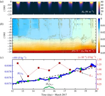
Observations in the ice-covered Lake Onego (Russia) from 12th to 20th of March 2017. (a) Solar irradiance
 $H_{0}$
in the water column, (b) density field,
 $\unicode[STIX]{x1D70C}(z,t)$
, relative to the density at the ice–water interface,
 $\unicode[STIX]{x1D70C}_{0}$
. (c) Background potential energy
 $\langle E_{b}\rangle _{Np}$
(blue line, left vertical axis), linear fitting (black dashed line, left vertical axis), diurnally averaged
 $\langle E_{b}\rangle _{N_{p}}$
(green circles, left vertical axis) and radiative energy,
 $E_{r,\unicode[STIX]{x1D70F}}$
(red squares, right vertical axis).

4 Application: observations in an ice-covered lake
The methodology developed in § 3.2 is applied to estimate
 $\unicode[STIX]{x1D702}_{c}$
using recent in situ, high-resolution observations from Lake Onego (Russia) during late Winter 2017 (Bouffard et al.
Reference Bouffard, Zdorovennova, Bogdanov, Efremova, Lavanchy, Palshin, Terzhevik, Råman Vinnå, Volkov, Wüest, Zdorovennov and Ulloa2018). Here we consider the simplest scenario of one monitoring spot. Observations of under-ice solar irradiance, light, and density distribution over the water column allowed estimating the evolution of radiative buoyancy flux,
 $\unicode[STIX]{x1D6F7}_{r}$
, using (3.8) and the background potential energy,
 $E_{b}$
, using (3.6). During this time, light penetrated between 1 and 1.5 m deep and the solar irradiance,
 $H_{0}$
, at the ice–water interface reached up to
 $100~\text{W}~\text{m}^{-2}$
(figure 2
a). The vertical density distribution (figure 2
b) is well-characterised by vertical signature schematised in figure 1. It has a stable upper thermally controlled boundary layer (
 ${<}1$
m) joined to a well-mixed layer attributed to radiatively driven convection (
 ${\sim}10$
m), which in turn is lower bound by a weakly stratified layer. Temperatures spanned from 0 to
 $1.5\,^{\circ }\text{C}$
(from top to bottom), and conductivity showed low and constant magnitudes (
 $27.00\pm 0.07~\unicode[STIX]{x03BC}\text{S}~\text{cm}^{-1}$
,
 ${\approx}0.02$
PSU) over the measuring period.
Figure 2(c) shows the temporal evolution of the estimated background potential energy
 $\langle E_{b}\rangle _{N_{p}}$
(blue line linked to left vertical axis in units
 $+101~\text{J}~\text{kg}^{-1}$
). It is characterised by an average increment of
 $8\times 10^{-5}~\text{J}~\text{kg}^{-1}~\text{day}^{-1}$
(dashed line) and diurnally averaged values,
 $\langle E_{b}\rangle _{N_{p},\unicode[STIX]{x1D70F}}$
, in green circles. Also, red squares denote the diurnally integrated radiative buoyancy flux,
 $E_{r,\unicode[STIX]{x1D70F}}$
(right vertical axis in units
 $\times 10^{-4}~\text{J}~\text{kg}^{-1}$
). The cumulative mixing efficiency over the observed period,
 $\unicode[STIX]{x1D70F}=8$
days, was estimated as in (3.9), obtaining a value of
 $\unicode[STIX]{x1D702}_{c}\approx 0.65$
. We also estimated
 $\unicode[STIX]{x1D702}_{c}$
at diurnal scale,
 $\unicode[STIX]{x1D70F}=1$
day, finding a median of 0.74 and a standard deviation of 0.19. Despite this difference, we emphasise that both values of
 $\unicode[STIX]{x1D702}_{c}$
are higher than the mixing efficiency broadly reported in stratified shear flows (Peltier & Caulfield Reference Peltier and Caulfield2003; Wüest & Lorke Reference Wüest and Lorke2003; Gregg et al.
Reference Gregg, D’Asaro, Riley and Kunze2018), while the eight-days-based value of
 $\unicode[STIX]{x1D702}_{c}$
(as well as the its median value) is remarkably close to those values found in buoyancy-driven mixing (e.g., Hughes et al.
Reference Hughes, Gayen and Griffiths2013; Davies Wykes & Dalziel Reference Davies Wykes and Dalziel2014; Sohail et al.
Reference Sohail, Gayen and Hogg2018). Indeed, our results are consistent with the theoretical findings of Davies Wykes et al. (Reference Davies Wykes, Hughes and Dalziel2015), who showed that in buoyancy-driven mixing
 $\unicode[STIX]{x1D702}_{c}$
can be higher than
 $1/2$
if there is stratification below the mixed layer. Longer time series and denser monitoring in smaller ice-covered lakes may be able to provide statistically more accurate estimations of
 $\unicode[STIX]{x1D702}_{c}$
in the future.
5 Concluding remarks
This paper introduces a framework to examine the mechanical energy budget and the mixing efficiency of radiatively forced, ice-covered Boussinesq flows. The theoretical formulation relies on the following assumptions.
(i) The fluid is confined to an ice-covered enclosed basin, meaning there is no advective exchange across boundaries. The model can be expanded to include (advective/diffusive) boundary fluxes in mechanical energy components. For instance, the bottom boundary could be forced by geothermal fluxes (Kirillin et al. Reference Kirillin, Leppäranta, Terzhevik, Granin, Bernhardt, Engelhardt, Efremova, Golosov, Palshin, Sherstyankin, Zdorovennova and Zdorovennov2012; Rizk et al. Reference Rizk, Kirillin and Leppäranta2014).
(ii) The Boussinesq density increases with temperature so
$\unicode[STIX]{x1D70C}\leqslant \unicode[STIX]{x1D70C}_{max}$
(freshwater basin). However, the presence of fully mixed water constituents (e.g., salinity) does not change the theoretical framework. Different equations of state (see appendix A) can be investigated via numerical approaches (ongoing work).(iii) Radiative forcing is parametrised by a monochromatic light attenuation depth scale,
$\unicode[STIX]{x1D706}$
. More sophisticated models considering the light-spectrum distribution can be readily adopted (Mironov et al.
Reference Mironov, Terzhevik, Kirillin, Jonas, Malm and Farmer2002; Bouffard et al.
Reference Bouffard, Zdorovennova, Bogdanov, Efremova, Lavanchy, Palshin, Terzhevik, Råman Vinnå, Volkov, Wüest, Zdorovennov and Ulloa2018) and would change the
$z$
-dependent function in
$F_{r}$
(3.7).


This work has three key outcomes.
(i) In § 2, we show that the radiative buoyancy flux,
$\unicode[STIX]{x1D6F7}_{r}$
, is a source of available mechanical energy and the fundamental driver in an ice-covered enclosed waterbody.(ii) In § 3, we formulate the cumulative mixing efficiency
$\unicode[STIX]{x1D702}_{c}$
to quantify the change in background potential energy from the supplied radiative energy at relevant time scales. We further suggest a handy field-based methodology to estimate
$\unicode[STIX]{x1D702}_{c}$
providing its scope.(iii) Results in § 4 illustrate a practical application of our framework and present a first estimation of the cumulative mixing efficiency in an ice-covered lake,
$\unicode[STIX]{x1D702}_{c}\approx 0.65$
. This value indicates that RDC in ice-covered lakes might be attributed to strong mixing regimes.


Still, similar to shear-driven mixing, depending on the integration time scale,
 $\unicode[STIX]{x1D70F}$
, and the turbulence age (Mashayek et al.
Reference Mashayek, Salehipour, Bouffard, Caulfield, Ferrari, Nikurashin, Peltier and Smyth2017),
 $\unicode[STIX]{x1D702}_{c}$
might vary over the course of the ice-covered season. The potential variability of
 $\unicode[STIX]{x1D702}_{c}$
is fostered by the fact that the background temperature/density distributions is changing in time. This change is particularly critical in the well-mixed layer whose temperature tends to
 $T_{md}\approx 4\,^{\circ }\text{C}$
. In this scenario, we might expect a drop of
 $\unicode[STIX]{x1D702}_{c}$
because of two reasons. First, the thermal expansion coefficient,
 $\unicode[STIX]{x1D6FC}_{T}\equiv \unicode[STIX]{x1D70C}_{0}^{-1}\unicode[STIX]{x2202}\unicode[STIX]{x1D70C}/\unicode[STIX]{x2202}T$
(see appendix A), decays as
 $T\rightarrow T_{md}$
, implying that the radiative-buoyancy-induced flux,
 $F_{r}$
, becomes weaker in magnitude as
 $T\rightarrow T_{md}$
. Secondly, the water column below the TBL tends to become fully mixed (e.g., Kirillin et al.
Reference Kirillin, Leppäranta, Terzhevik, Granin, Bernhardt, Engelhardt, Efremova, Golosov, Palshin, Sherstyankin, Zdorovennova and Zdorovennov2012; Salonen et al.
Reference Salonen, Pulkkanen, Salmi and Griffiths2014). Then, using the same theoretical arguments by Davies Wykes et al. (Reference Davies Wykes, Hughes and Dalziel2015),
 $\unicode[STIX]{x1D702}_{c}$
would tend to
 $1/2$
. Certainly, further studies are required for a deeper exploration of mixing regimes in ice-covered systems.
Despite the similarities between the RDC and the classical Rayleigh–Bénard convection (Hughes et al.
Reference Hughes, Gayen and Griffiths2013) and Rayleigh–Taylor instability (Davies Wykes & Dalziel Reference Davies Wykes and Dalziel2014), the magnitude of
 $\unicode[STIX]{x1D702}_{c}$
, the forcing mechanism (figures 1
b and 2
a), and the signature of density profiles shown in figure 2(b), suggest that RDC might be controlled by Rayleigh–Taylor like instabilities, especially in zones far from the basin lateral boundaries. In real systems, however, the basin topography can set cross-shore buoyancy gradients and so drive downslope flow (Kirillin et al.
Reference Kirillin, Forrest, Graves, Fischer, Engelhardt and Laval2015), similarly to those induced by night-time cooling in ice-free systems (Wells & Sherman Reference Wells and Sherman2001). Moreover, in large lakes, Coriolis force can affect cross-shore flows establishing, for instance, geostrophic circulations and localised gyres (Forrest et al.
Reference Forrest, Laval, Pieters and Lim2013; Rizk et al.
Reference Rizk, Kirillin and Leppäranta2014). In the aforementioned scenario,
 $\unicode[STIX]{x1D702}_{c}$
might show similar values to those reported in studies associated with the ocean overturning circulation (Barkan et al.
Reference Barkan, Winters and Llewellyn Smith2013; Vreugdenhil et al.
Reference Vreugdenhil, Gayen and Griffiths2016; Sohail et al.
Reference Sohail, Gayen and Hogg2018). The energy distribution and the global
 $\unicode[STIX]{x1D702}_{c}$
require to be systematically examined in the various mentioned scenarios. As suggested by Gregg et al. (Reference Gregg, D’Asaro, Riley and Kunze2018) regarding the ocean’s mixing problem, future works should further consider parametrisations based on relevant turbulence intensity parameters such as the Rayleigh number, the Reynolds buoyancy number, and the gradient Richardson number.
Quantifying the energetics and mixing in ice-covered waters is not only relevant for inferring the distribution of water constituents, but also for establishing the evolution of the ice cover (Kirillin et al.
Reference Kirillin, Leppäranta, Terzhevik, Granin, Bernhardt, Engelhardt, Efremova, Golosov, Palshin, Sherstyankin, Zdorovennova and Zdorovennov2012). MacKay et al. (Reference MacKay, Verseghy, Fortin and Rennie2017) and Yang et al. (Reference Yang, Young, Brown and Wells2017) suggested that strong vertical mixing can enhance the surface buoyancy flux,
 $\unicode[STIX]{x1D6F7}_{b}$
, across the ice–water interface and thus potentially influence the ice break. In this work, we show that
 $\unicode[STIX]{x1D6F7}_{b}$
relies on the TBL structure under the ice, which in turn depends on the radiative-buoyancy-induced flux,
 $F_{r}$
, and the temperature of the adjacent well-mixed layer (see figure 1
b). In particular, we notice that the optical properties of waters can significantly affect the light distribution and hence
 $F_{r}$
. In effect, for a same solar irradiance flux reaching the ice–water interface,
 $H_{0}$
, dark colour waters (such as Boreal lakes) tend to concentrate more heat in the very top of the water column than clear waters (such as pristine Alpine lakes). The above fact implies that not only the radiative buoyancy flux,
 $\unicode[STIX]{x1D6F7}_{r}$
, but also
 $\unicode[STIX]{x1D6F7}_{b}$
, can be modified depending on the water colour and the light distribution (Bouffard et al.
Reference Bouffard, Zdorovennova, Bogdanov, Efremova, Lavanchy, Palshin, Terzhevik, Råman Vinnå, Volkov, Wüest, Zdorovennov and Ulloa2018). Investigating the impact of the optical properties of water on
 $\unicode[STIX]{x1D6F7}_{b}$
and
 $\unicode[STIX]{x1D6F7}_{r}$
, and overall on mixing, might provide valuable information for determining the lifespan and sensibility of the ice cover in waterbodies.
Finally, we argue that the isolated conditions of ice-covered lakes make these systems particularly suitable for connecting lab and numerical studies to field scale. This work provides a framework to continue the exploration of physical processes in ice-covered waterbodies.
Acknowledgements
The in situ data used here were collected during a multidisciplinary research project supported by FEEL Foundation and are published by Bouffard et al. (Reference Bouffard, Zdorovennova, Bogdanov, Efremova, Lavanchy, Palshin, Terzhevik, Råman Vinnå, Volkov, Wüest, Zdorovennov and Ulloa2018). We thank the scientific and technical support from NWPI and KRC (Russ. Acad. Sci.). Finally, we are grateful for the support of three reviewers who contributed with outstanding observations and suggestions.
Appendix A. Equation of state and its impact on
$F_{r}$
and
$\unicode[STIX]{x1D6F7}_{r}$


The radiative-induced density flux,
 $F_{r}$
, that forces the mass transport equation (2.1a,b
), depends on the radiative heating distribution across the water column and the thermal expansion coefficient,
 $\unicode[STIX]{x1D6FC}_{T}$
. The last parameter sets the equation of state (EoS) of the fluid. In the case of a Boussinesq fluid (here, freshwater), a nonlinear EoS can be parametrised as follows:
 $$\begin{eqnarray}\unicode[STIX]{x1D70C}\equiv \unicode[STIX]{x1D70C}_{0}{\mathcal{P}}_{n}(T,\boldsymbol{x},t)\quad \text{and}\quad \unicode[STIX]{x1D6FC}_{T}\equiv \unicode[STIX]{x1D70C}_{0}^{-1}\unicode[STIX]{x2202}\unicode[STIX]{x1D70C}/\unicode[STIX]{x2202}T=\unicode[STIX]{x2202}{\mathcal{P}}_{n}/\unicode[STIX]{x2202}T={\mathcal{G}}_{n-1}(T,\boldsymbol{x},t),\end{eqnarray}$$
where
 ${\mathcal{P}}_{n}$
is a dimensionless polynomial of order
 $n$
,
 $T$
is the temperature field,
 $\unicode[STIX]{x1D6FC}_{T}$
is the general thermal expansion coefficient characterised by a temperature-dependent polynomial of order
 $n-1$
,
 ${\mathcal{G}}_{n-1}$
. Then,
 $F_{r}$
can be expressed as
 $$\begin{eqnarray}F_{r}=\unicode[STIX]{x1D6FC}_{T}(T,\boldsymbol{x},t)\frac{H_{0}(t)}{c_{p}}\text{e}^{z/\unicode[STIX]{x1D706}}=F_{0}(T,\boldsymbol{x},t)\text{e}^{z/\unicode[STIX]{x1D706}},\end{eqnarray}$$
where
 $H_{0}(t)\text{e}^{z/\unicode[STIX]{x1D706}}$
is the temporal and vertical radiative heating distribution and
 $c_{p}$
is the heat capacity of water. Thus, the radiative buoyancy flux per unit mass is given by
 $\unicode[STIX]{x1D6F7}_{r}\equiv g\unicode[STIX]{x1D70C}_{0}^{-1}\langle z\unicode[STIX]{x1D735}F_{r}\rangle _{V}$
, where
 $\unicode[STIX]{x1D735}$
is the divergence.
In the case of waters found between
 $0\,^{\circ }\text{C}\leqslant T<2\,^{\circ }\text{C}$
, a linear EoS captures reasonably well the relation between temperature and density. In this scenario,
 $\unicode[STIX]{x1D6FC}_{T}$
is a positive constant. Therefore,
 $F_{r}$
can be expressed as
 $F_{r}(z,t)=(\unicode[STIX]{x1D6FC}_{T}/c_{p})H_{0}(t)\text{e}^{z/\unicode[STIX]{x1D706}}$
, and the radiative buoyancy flux is reduced to
 $\unicode[STIX]{x1D6F7}_{r}\equiv g\unicode[STIX]{x1D70C}_{0}^{-1}\langle (\unicode[STIX]{x1D6FC}_{T}/c_{p})(H_{0}(t)/\unicode[STIX]{x1D706})z\text{e}^{z/\unicode[STIX]{x1D706}}\rangle _{V}$
. However, a quadratic EoS can describe fairly well the range of temperature
 $0\,^{\circ }\text{C}\leqslant T\leqslant 4\,^{\circ }\text{C}$
. In this case,
 $\unicode[STIX]{x1D6FC}_{T}$
is characterised by a linear function of the temperature, and reaches a minimum at the temperature of maximum density.