1 Introduction
Turbulent flows are ubiquitous in the environment, where the accurate prediction of turbulent transport of momentum, heat, water vapour and other passive scalars has practical importance for diverse applications such as renewable energy (Calaf, Meneveau & Meyers Reference Calaf, Meneveau and Meyers2010; Calaf, Parlange & Meneveau Reference Calaf, Parlange and Meneveau2011), urban meteorology (Cheng & Castro Reference Cheng and Castro2002; Coceal et al.
Reference Coceal, Dobre, Thomas and Belcher2007; Philips, Rossi & Iaccarino Reference Philips, Rossi and Iaccarino2013; Anderson, Li & Bou-Zeid Reference Anderson, Li and Bou-Zeid2015; Giometto et al.
Reference Giometto, Christen, Meneveau, Fang, Krafczyk and Parlange2016, Reference Giometto, Christen, Egli, Schmid, Tooke, Coops and Parlange2017), transport within vegetation canopies (Chester, Meneveau & Parlange Reference Chester, Meneveau and Parlange2007; Chamecki, Meneveau & Parlange Reference Chamecki, Meneveau and Parlange2009; Finnigan, Shaw & Patton Reference Finnigan, Shaw and Patton2009; Bailey & Stoll Reference Bailey and Stoll2013), flow over complex landscapes (Bou-Zeid, Meneveau & Parlange Reference Bou-Zeid, Meneveau and Parlange2005; Anderson & Meneveau Reference Anderson and Meneveau2011; Anderson & Chamecki Reference Anderson and Chamecki2014) and evapotranspiration (Penman Reference Penman1948; Brutsaert & Stricker Reference Brutsaert and Stricker1979; Parlange, Eichinger & Albertson Reference Parlange, Eichinger and Albertson1995). These flows are notable for their ‘asymptotic’ inertial conditions, where turbulence is produced by mechanical shear (i.e.
 $Re_{\unicode[STIX]{x1D70F}}=u_{\unicode[STIX]{x1D70F}}z_{i}/\unicode[STIX]{x1D708}\sim O(10^{7})$
, where
 $u_{\unicode[STIX]{x1D70F}}$
is the shear velocity,
 $z_{i}$
is the flow depth and
 $\unicode[STIX]{x1D708}$
is the kinematic viscosity) and buoyancy (low Richardson number), and influenced by Coriolis accelerations (low Rossby number). One key challenge in atmospheric science and related disciplines is developing accurate models to represent the effects of turbulent transport in weather, climate and hydrological prediction models. The main scaling hypothesis that has served as a cornerstone of atmospheric boundary layer research for over half a century is Monin–Obukhov (MO) similarity theory (Obukhov Reference Obukhov1946; Monin & Obukhov Reference Monin and Obukhov1954), developed for an atmospheric surface layer (or ASL, the lowest 10–15 % of the atmospheric boundary layer) over flat, horizontally homogeneous terrain. MO similarity introduces a correction to the logarithmic law of the wall to account for the effects of thermal stratification. Under the MO hypothesis, the wall-normal distance
 $z$
, the friction velocity
 $u_{\unicode[STIX]{x1D70F}}$
, the buoyancy parameter
 $g/\unicode[STIX]{x1D6E9}_{0}$
and the kinematic surface heat flux
 $Q_{0}=\overline{w^{\prime }\unicode[STIX]{x1D703}^{\prime }}$
are taken to be the relevant scales in the dimensional analysis (where
 $\unicode[STIX]{x1D703}$
is potential temperature,
 $\unicode[STIX]{x1D6E9}_{0}$
is a reference potential temperature and
 $g$
is acceleration due to gravity.) Upon applying the Buckingham
 $\unicode[STIX]{x03A0}$
theorem, one can show that a statistical quantity of interest normalized by the MO scales (
 $\unicode[STIX]{x1D719}$
) is predicted to depend on only the MO stability parameter (
 $\unicode[STIX]{x1D701}=z/L$
), where
 $$\begin{eqnarray}L=\frac{-u_{\unicode[STIX]{x1D70F}}^{3}\unicode[STIX]{x1D6E9}_{0}}{\unicode[STIX]{x1D705}gQ_{0}}\end{eqnarray}$$
is the Obukhov length and
 $\unicode[STIX]{x1D705}$
is the von Kármán constant. Use of MO similarity is widespread in the atmospheric and hydrologic sciences and related disciplines, where it is used to estimate turbulent fluxes of quantities that cannot be measured directly by eddy covariance (Baldocchi, Hincks & Meyers Reference Baldocchi, Hincks and Meyers1988; Cline Reference Cline1997; Moncrieff et al.
Reference Moncrieff, Valentini, Greco, Guenther and Ciccioli1997), to parametrize turbulent fluxes in numerical weather, climate and hydrological forecasting models (e.g. Deardorff Reference Deardorff1972b
; Louis Reference Louis1979), and to impose the lower boundary condition in large eddy simulations of the atmospheric boundary layer (e.g. Deardorff Reference Deardorff1972a
; Moeng Reference Moeng1984; Kumar et al.
Reference Kumar, Kleissl, Meneveau and Parlange2006). In this article we shall denote the streamwise, spanwise and wall-normal coordinates as
 $\boldsymbol{x}=\{x,y,z\}$
, with velocity components
 $\boldsymbol{u}=\{u,v,w\}$
. Resolved-scale quantities from the large eddy simulations (LES) we shall consider in this work will be denoted with a tilde, e.g.
 $\widetilde{\boldsymbol{u}}=\{\widetilde{u},\widetilde{v},\widetilde{w}\}$
. We furthermore shall use the Reynolds averaging convention, where a total resolved-scale variable is decomposed into ensemble mean and fluctuating parts, e.g.
 $\widetilde{a}=A+\widetilde{a}^{\prime }$
.
The framework provided by MO similarity has been highly successful for predicting the statistics of many turbulent quantities, including the dimensionless mean wind shear
 $\unicode[STIX]{x1D719}_{m}$
and temperature gradient
 $\unicode[STIX]{x1D719}_{h}$
(Businger et al.
Reference Businger, Wyngaard, Izumi and Bradley1971; Högström Reference Högström1988), velocity and temperature spectra under stable conditions (Kaimal et al.
Reference Kaimal, Wyngaard, Izumi and Coté1972; Kaimal & Finnigan Reference Kaimal and Finnigan1994), the vertical velocity spectrum under unstable conditions (Kaimal et al.
Reference Kaimal, Wyngaard, Izumi and Coté1972) and the vertical velocity and temperature variances under unstable and stable conditions (Kaimal & Finnigan Reference Kaimal and Finnigan1994). (Some quantities such as the variances and spectra of the horizontal velocity components are known not to be MO-similar; e.g. see Kaimal et al. (Reference Kaimal, Wyngaard, Izumi and Coté1972) and Panofsky et al. (Reference Panofsky, Tennekes, Lenschow and Wyngaard1977).) However, over the past several decades an alternative view of wall turbulence has emerged that has cast the discussion of turbulent transport in terms of organized (or coherent) structures, which are persistent in space and time and can be responsible for a significant fraction (50 % or more) of the momentum flux and turbulent kinetic energy close to the wall (Corino & Brodkey Reference Corino and Brodkey1969; Wallace, Eckelmann & Brodkey Reference Wallace, Eckelmann and Brodkey1972; Willmarth & Lu Reference Willmarth and Lu1972; Guala, Hommema & Adrian Reference Guala, Hommema and Adrian2006; Balakumar & Adrian Reference Balakumar and Adrian2007; Wallace Reference Wallace2016). These structures are significant, as their spatial extent far exceeds the depth of the flow,
 $z_{i}$
. This evolution in perspective has been influenced by findings in the fundamental wall turbulence community.
In order to meaningfully compare atmospheric boundary layer (ABL) turbulence with canonical smooth-wall turbulent boundary layers, brief remarks are needed on the vertical structure of both flows. The ABL, which exhibits asymptotically large
 $Re_{\unicode[STIX]{x1D70F}}$
, is comprised of a shear-dominated inner (or surface) layer (
 $0\lesssim z/z_{i}\lesssim 0.1$
) and a buoyancy- and Coriolis-influenced inertial layer (
 $z/z_{i}\gtrsim 0.1$
). In contrast, canonical smooth-wall turbulent boundary layers are comprised of a viscous-dominated inner layer, which resides beneath the outer (logarithmic) layer (the presence of outer-layer structures is predicated upon
 $Re_{\unicode[STIX]{x1D70F}}$
, where preceding studies have reported
 $Re_{\unicode[STIX]{x1D70F}}\gtrsim 2000$
as a threshold for the formation of large-scale outer-layer motions; (Hutchins & Marusic Reference Hutchins and Marusic2007a
)). The viscous-dominated inner layer is occupied by an inner cycle (Kline et al.
Reference Kline, Reynolds, Schraub and Runstadler1967; Bandyopadhyay & Hussain Reference Bandyopadhyay and Hussain1984; Schoppa & Hussain Reference Schoppa and Hussain2002; Del Alamo et al.
Reference Del Alamo, Jiménez, Zandonade and Moser2004), which has now been well studied with experimental measurement and numerical simulation. The extent to which the inner and outer layer are coupled is, itself, the topic of ongoing inquiry.
Autogeneration processes within the inner layer, in which hairpin vortices (Theodorsen Reference Theodorsen1952; Head & Bandyopadhyay Reference Head and Bandyopadhyay1981; Adrian Reference Adrian2007) eject low-momentum fluid vertically (
 $u^{\prime }<0$
,
 $w^{\prime }>0$
), thereby initiating the formation of successive hairpins encapsulating zones of relatively low-momentum fluid, has been well studied (Meinhart & Adrian Reference Meinhart and Adrian1995). On the other hand, large-scale structures in the logarithmic or outer layer can influence small-scale turbulence in the inner layer through sweeps of high-momentum fluid toward the wall (
 $u^{\prime }>0$
,
 $w^{\prime }<0$
) Studies over the past several decades (Kovasznay, Kibens & Blackwelder Reference Kovasznay, Kibens and Blackwelder1970; Brown & Thomas Reference Brown and Thomas1977; Nakagawa & Nezu Reference Nakagawa and Nezu1981; Murlis, Tsai & Bradshaw Reference Murlis, Tsai and Bradshaw1982; McLean Reference McLean1990; Wark & Nagib Reference Wark and Nagib1991; Adrian, Meinhart & Tomkins Reference Adrian, Meinhart and Tomkins2000; Ganapathisubramani, Longmire & Marusic Reference Ganapathisubramani, Longmire and Marusic2003; Tomkins & Adrian Reference Tomkins and Adrian2003; Del Alamo et al.
Reference Del Alamo, Jiménez, Zandonade and Moser2004) have focused on these so-called large-scale motions (LSMs), elongated regions of high- and low-momentum fluid present in the logarithmic layer at high Reynolds numbers that extend approximately
 $O(z_{i})$
in the streamwise direction. LSMs are attributed to packets of hairpin vortices that occur in streamwise succession, have similar propagation speeds, and increase in size in the streamwise direction (e.g. Adrian Reference Adrian2007).
More recently, studies have also identified so-called very-large-scale motions (VLSM), elongated regions in the logarithmic layer that extend
 $O(10\,z_{i})$
in the streamwise direction (Kim & Adrian Reference Kim and Adrian1999; Guala et al.
Reference Guala, Hommema and Adrian2006; Balakumar & Adrian Reference Balakumar and Adrian2007; Hutchins & Marusic Reference Hutchins and Marusic2007a
; Marusic & Hutchins Reference Marusic and Hutchins2008) and occur due to streamwise coalescence of hairpin vortex packets. VLSMs can be detected from the outer peak in the premultiplied streamwise velocity spectra (Kim & Adrian Reference Kim and Adrian1999). They may exhibit spanwise meandering in the instantaneous velocity field (Hutchins & Marusic Reference Hutchins and Marusic2007a
), and have a significant influence on the near-wall cycle through modulation of small-scale turbulent fluctuations (Mathis, Hutchins & Marusic Reference Mathis, Hutchins and Marusic2009a
; Chung & McKeon Reference Chung and McKeon2010). The initial identification of VLSMs and subsequent studies in turbulent channel flow (Del Alamo et al.
Reference Del Alamo, Jiménez, Zandonade and Moser2004; Chung & McKeon Reference Chung and McKeon2010), pipe flow (Guala et al.
Reference Guala, Hommema and Adrian2006; Wu, Baltzer & Adrian Reference Wu, Baltzer and Adrian2012) and boundary layers (Tomkins & Adrian Reference Tomkins and Adrian2003; Hambleton, Hutchins & Marusic Reference Hambleton, Hutchins and Marusic2006; Hutchins & Marusic Reference Hutchins and Marusic2007a
,Reference Hutchins and Marusic
b
; Lee & Sung Reference Lee and Sung2011) did not occur until recently due to limitations in the Reynolds numbers attainable in laboratory studies and direct numerical simulations (Marusic et al.
Reference Marusic, McKeon, Monkewitz, Nagib, Smits and Sreenivasan2010b
). VLSMs have also been observed in the near-neutrally stratified atmospheric surface layer (Kunkel & Marusic Reference Kunkel and Marusic2006; Hutchins & Marusic Reference Hutchins and Marusic2007a
; Guala & McKeon Reference Guala and McKeon2011; Hutchins et al.
Reference Hutchins, Chauhan, Marusic, Monty and Klewicki2012; Fang & Porté-Agel Reference Fang and Porté-Agel2015; Jacob & Anderson Reference Jacob and Anderson2017) at high Reynolds number (
 $\mathit{Re}\sim O(10^{7}{-}10^{8})$
). A comprehensive discussion of these structures can be found in several review articles in the literature (Cantwell Reference Cantwell1981; Robinson Reference Robinson1991; Panton Reference Panton2001; Adrian Reference Adrian2007; Marusic et al.
Reference Marusic, McKeon, Monkewitz, Nagib, Smits and Sreenivasan2010b
; Jiménez Reference Jiménez2018). This article is directed towards the study of LSMs and VLSMs in inertia-dominated (high
 $Re_{\unicode[STIX]{x1D70F}}$
), rotating (low Rossby number,
 $Ro$
), unstably stratified (low Richardson number,
 $Ri$
) ABL turbulence. This general combination of parameters encompasses a wide variety of important geophysical flows, although herein we choose cases replicating turbulence in terrestrial planetary boundary layers.
Both LSMs and VLSMs have received an increasing amount of attention in recent studies of turbulence in smooth-walled channels, boundary layers and pipes due to the observation that they modulate the amplitude (Mathis et al. Reference Mathis, Hutchins and Marusic2009a ,Reference Mathis, Monty, Hutchins and Marusic b ; Marusic, Mathis & Hutchins Reference Marusic, Mathis and Hutchins2010a ) and frequency (Ganapathisubramani et al. Reference Ganapathisubramani, Hutchins, Monty, Chung and Marusic2012; Baars et al. Reference Baars, Talluru, Hutchins and Marusic2015; Baars, Hutchins & Marusic Reference Baars, Hutchins and Marusic2016, Reference Baars, Hutchins and Marusic2017; Pathikonda & Christensen Reference Pathikonda and Christensen2017; Awasthi & Anderson Reference Awasthi and Anderson2018) of small-scale turbulent fluctuations. This observation has led to the development of a simple predictive model for flow statistics in the inner layer (Marusic et al. Reference Marusic, Mathis and Hutchins2010a ; Mathis, Hutchins & Marusic Reference Mathis, Hutchins and Marusic2011), requiring as the only input the large-scale velocity signal from the outer region. Other studies have demonstrated that this amplitude modulation phenomenon is not restricted to turbulent shear flows over smooth walls, but also occurs in rough-wall turbulent flows (Anderson Reference Anderson2016; Squire et al. Reference Squire, Baars, Hutchins and Marusic2016; Pathikonda & Christensen Reference Pathikonda and Christensen2017; Awasthi & Anderson Reference Awasthi and Anderson2018). Further motivation for investigating LSMs and VLSMs has come from recent studies in wall turbulence (Marusic & Kunkel Reference Marusic and Kunkel2003; Hultmark et al. Reference Hultmark, Vallikivi, Bailey and Smits2012; Marusic et al. Reference Marusic, Monty, Hultmark and Smits2013) that have provided evidence that that the profile of streamwise turbulent fluctuations in the inertial region can be described by a universal scaling law of the form
 $$\begin{eqnarray}\frac{\overline{u^{\prime 2}}}{u_{\unicode[STIX]{x1D70F}}^{2}}=B_{1}-A_{1}\ln (z/z_{i}),\end{eqnarray}$$
based on predictions from the attached eddy hypothesis (Townsend Reference Townsend1976; Perry & Chong Reference Perry and Chong1982; Perry, Henbest & Chong Reference Perry, Henbest and Chong1986). Although the data support a universal value of
 $A_{1}\approx 1.25$
(Marusic & Kunkel Reference Marusic and Kunkel2003; Smits, McKeon & Marusic Reference Smits, McKeon and Marusic2011; Hultmark et al.
Reference Hultmark, Vallikivi, Bailey and Smits2012; Marusic et al.
Reference Marusic, Monty, Hultmark and Smits2013),
 $B_{1}$
has been found to be dependent on flow conditions and geometry (e.g. Marusic et al.
Reference Marusic, Monty, Hultmark and Smits2013; Meneveau & Marusic Reference Meneveau and Marusic2013). Recently Banerjee & Katul (Reference Banerjee and Katul2013) used a spectral budget model to connect
 $B_{1}$
to the largest scales of motion in a wall-bounded flow suggesting that VLSMs are responsible for the non-universal behaviour of
 $B_{1}$
and thus contribute to the mean profile of
 $\overline{u^{\prime 2}}$
. In the atmospheric boundary layer, the corresponding hypothesis is that the failure of the horizontal velocity variances and spectra to follow MO similarity (Kaimal et al.
Reference Kaimal, Wyngaard, Izumi and Coté1972; Panofsky et al.
Reference Panofsky, Tennekes, Lenschow and Wyngaard1977) is due to the presence of VLSMs (e.g. Banerjee et al.
Reference Banerjee, Katul, Salesky and Chamecki2015). While much of the aforementioned work has been devoted to understanding the extent to which LSMs and VLSMs modulate flow statistics in the viscous sublayer of flows over smooth walls, the focus of the present work is on how large-scale coherent structures in the outer layer modulate small-scale turbulence in the roughness sublayer in unstably stratified wall turbulence over aerodynamically rough surfaces.
1.1 Effects of unstable stratification
Because turbulence statistics and coherent structures both undergo significant changes as a fluid becomes unstably stratified, it is unclear whether previous results on modulation phenomena and inner–outer interactions in neutrally stratified turbulent shear flows can be extended to the unstably stratified case. Buoyancy has significant effects on many properties of turbulence, including the integral scales (Kaimal et al.
Reference Kaimal, Wyngaard, Izumi and Coté1972; Sullivan et al.
Reference Sullivan, Horst, Lenschow, Moeng and Weil2003; Salesky, Katul & Chamecki Reference Salesky, Katul and Chamecki2013), the turbulent kinetic energy (TKE) budget and the partitioning of TKE between its components (
 $\overline{u^{\prime 2}}$
,
 $\overline{v^{\prime 2}}$
and
 $\overline{w^{\prime 2}}$
) (Wyngaard & Coté Reference Wyngaard and Coté1971; Frenzen & Vogel Reference Frenzen and Vogel1992, Reference Frenzen and Vogel2001; Salesky, Chamecki & Bou-Zeid Reference Salesky, Chamecki and Bou-Zeid2017), the velocity and temperature spectra (Kaimal et al.
Reference Kaimal, Wyngaard, Izumi and Coté1972; Kaimal & Finnigan Reference Kaimal and Finnigan1994) and the structure functions (Chamecki et al.
Reference Chamecki, Dias, Salesky and Pan2017).
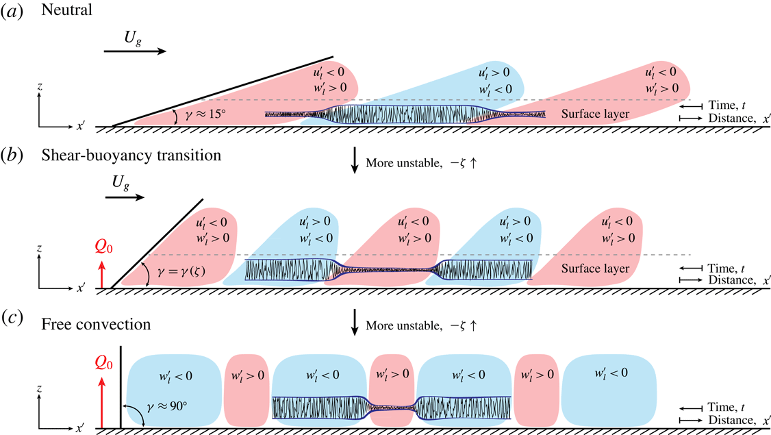
In addition to changes in mean properties of turbulence, significant changes in coherent structures also occur due to buoyancy. In neutrally stratified flows, the inclination angle of structures in the logarithmic region (interpreted as the inclination of hairpin vortex packets from the horizontal, Brown & Thomas Reference Brown and Thomas1977) is typically found to be
 $\unicode[STIX]{x1D6FE}=15^{\circ }$
(Carper & Porté-Agel Reference Carper and Porté-Agel2004; Marusic & Heuer Reference Marusic and Heuer2007) and invariant with respect to Reynolds number (Marusic & Heuer Reference Marusic and Heuer2007). The inclination angle has been investigated through two-point correlations of streamwise velocity, or cross-correlations between streamwise velocity and surface shear stress (with lags in the streamwise and wall-normal directions) (e.g. Kovasznay et al.
Reference Kovasznay, Kibens and Blackwelder1970; Brown & Thomas Reference Brown and Thomas1977; Rajagopalan & Antonia Reference Rajagopalan and Antonia1979; Boppe & Neu Reference Boppe and Neu1995; Christensen & Adrian Reference Christensen and Adrian2001; Carper & Porté-Agel Reference Carper and Porté-Agel2004; Ganapathisubramani et al.
Reference Ganapathisubramani, Hutchins, Hambleton, Longmire and Marusic2005; Marusic & Heuer Reference Marusic and Heuer2007; Morris et al.
Reference Morris, Stolpa, Slaboch and Klewicki2007; Hutchins et al.
Reference Hutchins, Chauhan, Marusic, Monty and Klewicki2012). The structure inclination angle emerges as a parameter in some wall models for LES (Piomelli et al.
Reference Piomelli, Ferziger, Moin and Kim1989; Marusic, Kunkel & Porté-Agel Reference Marusic, Kunkel and Porté-Agel2001) which have been found to have superior performance over models where the inclination angle is neglected (Piomelli et al.
Reference Piomelli, Ferziger, Moin and Kim1989; Piomelli & Balaras Reference Piomelli and Balaras2002). Furthermore,
 $\unicode[STIX]{x1D6FE}$
also appears as a parameter in a predictive model for streamwise velocity statistics in the near-wall region (Marusic et al.
Reference Marusic, Mathis and Hutchins2010a
; Mathis et al.
Reference Mathis, Hutchins and Marusic2011). As the atmosphere becomes increasingly unstable (increasing
 $-\unicode[STIX]{x1D701}$
), the inclination angle increases to
 $50^{\circ }$
or more (Hommema & Adrian Reference Hommema and Adrian2003; Carper & Porté-Agel Reference Carper and Porté-Agel2004; Chauhan et al.
Reference Chauhan, Hutchins, Monty and Marusic2013). This steepening is physically consistent with the underlying mechanism in which turbulent buoyant plumes change the momentum balance of the flow and induce a greater vertical transport. Moreover, since LSMs – presumed to be the ‘building blocks’ of which VLSMs are composed – are responsible for modulating near-wall dynamics, changes in their structural characteristics must have direct implications for amplitude modulation. In more direct terms, assume for discussion that each LSM has a height
 $z_{i}$
with inclination,
 $\unicode[STIX]{x1D6FE}$
. A cursory estimate for their length can then be deduced via
 $L_{1}=z_{i}/\tan (\unicode[STIX]{x1D6FE})\approx 3z_{i}$
. Individual LSMs generally undergo a quasi-streamwise coalescence (Kim & Adrian Reference Kim and Adrian1999; Balakumar & Adrian Reference Balakumar and Adrian2007; Dennis & Nickels Reference Dennis and Nickels2011a
,Reference Dennis and Nickels
b
), resulting in spatially meandering very-large-scale motions (VLSM) (Hutchins & Marusic Reference Hutchins and Marusic2007a
) with streamwise extent,
 $L_{2}/z_{i}\approx 21$
. The existence of VLSMs has been well documented in pipes (Lee & Sung Reference Lee and Sung2011; Hellström, Ganapathisubramania & Smits Reference Hellström, Ganapathisubramania and Smits2015), channels (Fang & Porté-Agel Reference Fang and Porté-Agel2015; Jacob & Anderson Reference Jacob and Anderson2017) and boundary layers (Ganapathisubramani et al.
Reference Ganapathisubramani, Longmire and Marusic2003; Wu & Christensen Reference Wu and Christensen2007, Reference Wu and Christensen2010).
Using LES results, Salesky et al. (Reference Salesky, Chamecki and Bou-Zeid2017) demonstrated that the root-mean-square (r.m.s.) horizontal resolved-scale vorticity in the ASL decreases with increasing bulk stability parameter
 $-z_{i}/L$
(where
 $z_{i}$
is the convective boundary-layer depth, i.e. the outer length scale), whereas the r.m.s. vertical resolved-scale vorticity increases with
 $-z_{i}/L$
(their figure 11). These prior observations suggest that surface layer structures become more steeply inclined with increasing
 $-\unicode[STIX]{x1D701}$
with hairpin vortex packets occurring under weakly convective conditions and vertical buoyant thermals (
 $\unicode[STIX]{x1D6FE}\approx 90^{\circ }$
) occurring in free convection. Visual evidence of hairpin vortex packets becoming inclined with increasing
 $-\unicode[STIX]{x1D701}$
was provided by Hommema & Adrian (Reference Hommema and Adrian2003) through smoke visualizations in the convective atmospheric surface layer.
Significant topological changes also occur in large-scale turbulent structures as the convective boundary layer (CBL) becomes increasingly unstable. When surface heat fluxes are small and mean shear is large (small values of
 $-z_{i}/L$
), updrafts in the convective boundary layer tend to organize into quasi-two-dimensional linear structures (often termed horizontal convective rolls, or HCRs) that are aligned within
 $10^{\circ }$
–
 $20^{\circ }$
of the geostrophic wind direction (supporting results can be found in § 3.2) (e.g. LeMone Reference LeMone1973, Reference LeMone1976; Moeng & Sullivan Reference Moeng and Sullivan1994; Weckwerth et al.
Reference Weckwerth, Wilson, Wakimoto and Crook1997; Weckwerth, Horst & Wilson Reference Weckwerth, Horst and Wilson1999; Khanna & Brasseur Reference Khanna and Brasseur1998; Young et al.
Reference Young, Kristovich, Hjelmfelt and Foster2002; Salesky et al.
Reference Salesky, Chamecki and Bou-Zeid2017). However, when surface heat fluxes are large, but mean wind shear is weak (large
 $-z_{i}/L$
), updrafts tend to organize into open cells (Agee, Chen & Dowell Reference Agee, Chen and Dowell1973; Atkinson & Zhang Reference Atkinson and Zhang1996; Salesky et al.
Reference Salesky, Chamecki and Bou-Zeid2017), similar to turbulent Rayleigh–Bénard convection in laboratory flows. The transition from horizontal convective rolls to open cells was investigated with LES by Salesky et al. (Reference Salesky, Chamecki and Bou-Zeid2017), who found that although the transition occurs gradually over a range of
 $-z_{i}/L$
, the most significant changes in large-scale structures occur from near-neutral conditions up to about
 $-z_{i}/L=15{-}20$
. This article is motivated by the overarching question: if LSMs are present for increasingly unstable conditions – albeit, with varied spatial characteristics across the range of
 $-z_{i}/L$
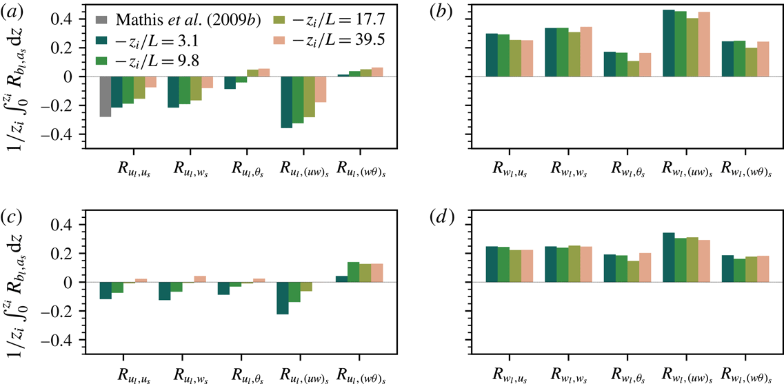
– should the conceptual arguments of amplitude modulation remain valid? Results demonstrate that inner-layer modulation by LSMs aloft continues to occur. However, modulation by large-scale streamwise velocity decreases monotonically with increasing
 $-z_{i}/L$
, whereas modulation by large-scale vertical velocity remains significant as long as there is sufficient scale separation between the inner and outer peaks in the spectrograms.
1.2 Amplitude modulation
In the present article, we shall employ the ‘decoupling procedure’ proposed by Mathis et al. (Reference Mathis, Hutchins and Marusic2009a ) for quantifying the extent to which amplitude modulation (AM) occurs. The decoupling procedure, which is based on the Hilbert transform, will be reviewed briefly below. We contend that evidence of AM based on this procedure serves as an indication that other measures of correlation (e.g. based on the wavelet transform, Baars et al. Reference Baars, Talluru, Hutchins and Marusic2015, Reference Baars, Hutchins and Marusic2017; Pathikonda & Christensen Reference Pathikonda and Christensen2017; Awasthi & Anderson Reference Awasthi and Anderson2018) would also indicate the presence of modulation of small-scale turbulence. We also calculated the AM coefficients using the method of Baars et al. (Reference Baars, Talluru, Hutchins and Marusic2015) based on the continuous wavelet transform. While some small quantitative differences in the two methods exist (e.g. Baars et al. Reference Baars, Talluru, Hutchins and Marusic2015; Awasthi & Anderson Reference Awasthi and Anderson2018), the qualitative results and overall conclusions are similar.
Consider two variables that are each a function of wall-normal distance and time, i.e.
 $a=a(z;t)$
and
 $b=b(z_{ref};t)$
, where we wish to determine the amplitude modulation of small-scale
 $a$
(at height
 $z$
) by large-scale
 $b$
(at some reference height
 $z_{ref}$
). First, the variables
 $a$
and
 $b$
are low-pass filtered to determine their respective large-scale components, e.g.
 $a_{l}(z;t)=G_{z_{i}}\star a(z;t)$
where
 $(\star )$
denotes convolution and
 $G_{z_{i}}$
is a filter function. We here employ a sharp spectral filter at cutoff scale
 $z_{i}$
, where
 $z_{i}$
again denotes the outer length scale (here the convective boundary-layer depth
 $z_{i}$
). Prior works have demonstrated that AM coefficients are not particularly sensitive to the choice of cutoff length scale employed, provided that the filter length corresponds with the spectral plateau separating the inner and outer peaks. The small-scale component of each variable is then calculated via
 $a_{s}(z;t)=a(z;t)-a_{l}(z;t)$
. Next, we compute the Hilbert transform of the small-scale
 $a$
:
 $$\begin{eqnarray}{\mathcal{A}}_{s}(t)={\mathcal{H}}\{a_{s}(t)\}=\frac{1}{\unicode[STIX]{x03C0}}{\mathcal{P}}\int _{-\infty }^{+\infty }\frac{a_{s}(\unicode[STIX]{x1D70F})}{t-\unicode[STIX]{x1D70F}}\,\text{d}\unicode[STIX]{x1D70F},\end{eqnarray}$$
where
 ${\mathcal{H}}$
denotes the Hilbert transform operator and
 ${\mathcal{P}}$
is the Cauchy principal value.
A few brief remarks regarding the Hilbert transform operator are appropriate here. From (1.3), one can see that
 ${\mathcal{A}}_{s}(t)$
is the convolution of the small-scale signal
 $a_{s}(t)$
with the quantity
 $(1/\unicode[STIX]{x03C0}t)$
, i.e.
 ${\mathcal{A}}_{s}(t)=a_{s}(t)\ast (1/\unicode[STIX]{x03C0}t)$
. From the Fourier convolution theorem, one can show (Mathis et al.
Reference Mathis, Hutchins and Marusic2009a
) that the Hilbert transformed signal
 ${\mathcal{A}}_{s}(t)$
is equal to the original signal
 $a_{s}(t)$
with Fourier components shifted
 $-\unicode[STIX]{x03C0}/2$
for positive frequencies and
 $+\unicode[STIX]{x03C0}/2$
for negative frequencies. (For a more in-depth discussion of the Hilbert transform, the reader is referred to Bendat & Piersol (Reference Bendat and Piersol2010). Use of the Hilbert transform to detect amplitude modulation in an idealized signal is presented in Mathis et al. (Reference Mathis, Hutchins and Marusic2009a
).) Thus
 $a_{s}(t)$
and
 ${\mathcal{A}}_{s}(t)$
form a harmonic conjugate pair and can be used to define the complex analytic signal
 $$\begin{eqnarray}{\mathcal{Z}}(t)=a_{s}(t)+\text{i}{\mathcal{A}}_{s}(t)=A(t)\text{e}^{\text{i}\unicode[STIX]{x1D719}(t)},\end{eqnarray}$$
which can be expressed in terms of an amplitude
 $A(t)$
and a phase
 $\unicode[STIX]{x1D719}(t)$
. From (1.4), one can see that the Hilbert transform is useful for extracting instantaneous amplitude and phase information from a temporal signal (e.g. Sreenivasan Reference Sreenivasan1985; Hristov, Friehe & Miller Reference Hristov, Friehe and Miller1998; Tardu Reference Tardu2008; Mathis et al.
Reference Mathis, Hutchins and Marusic2009a
). The envelope of the small-scale variable
 $a_{s}$
is given by the modulus of the complex analytic signal:
 $$\begin{eqnarray}E(a_{s})=A(t)=\sqrt{a_{s}^{2}(t)+{\mathcal{A}}_{s}^{2}(t)}\end{eqnarray}$$
(e.g. Mathis et al.
Reference Mathis, Hutchins and Marusic2009a
, and references therein). The envelope of
 $a_{s}$
is then low-pass filtered to determine its large-scale component, i.e.
 $E_{l}(a_{s})=G_{z_{i}}\star E(a_{s})$
. Finally, the AM coefficient is given by the correlation coefficient between the large-scale component of
 $b$
and the filtered envelope of small-scale
 $a$
:
 $$\begin{eqnarray}R_{b_{l},a_{s}}(z,z_{ref};z_{i}/L)=\frac{\overline{b_{l}^{\prime }(z_{ref};t+\unicode[STIX]{x1D6FF}\unicode[STIX]{x1D70F}(z;z_{ref}))E_{l}^{\prime }(a_{s}(z;t))}}{\sqrt{\overline{b_{l}^{\prime 2}(z_{ref};t+\unicode[STIX]{x1D6FF}\unicode[STIX]{x1D70F}(z;z_{ref}))}}\sqrt{\overline{E_{l}^{\prime 2}(a_{s}(z;t))}}}.\end{eqnarray}$$
Here
 $\unicode[STIX]{x1D6FF}\unicode[STIX]{x1D70F}(z;z_{ref})$
is an advective lag used to account for the structure inclination angle when calculating the two-point AM coefficient. It is defined as
 $$\begin{eqnarray}\unicode[STIX]{x1D6FF}\unicode[STIX]{x1D70F}(z;z_{ref})=\frac{z_{ref}-z}{U_{c}\tan \unicode[STIX]{x1D6FE}},\end{eqnarray}$$
where
 $z_{ref}$
is the reference height for the two-point AM coefficient,
 $U_{c}$
is a suitable convection velocity and
 $\unicode[STIX]{x1D6FE}$
is the inclination angle of structures in the atmospheric surface layer (Anderson et al.
Reference Anderson, Li and Bou-Zeid2015). It follows from inspection of (1.6) that for computation of the single-point correlation,
 $z_{ref}=z$
and
 $\unicode[STIX]{x1D6FF}\unicode[STIX]{x1D70F}(z;z_{ref})=0$
. In addition to dependence on height
 $z$
and reference height
 $z_{ref}$
, we shall demonstrate below that in the convective boundary layer the AM coefficient also depends on the global stability parameter
 $z_{i}/L$
. In the present work, we shall consider both single-point AM coefficients (i.e.
 $R_{b_{l},a_{s}}(z,z;z_{i}/L)$
) to determine how large-scale motions amplitude modulate small-scale turbulence at the same wall-normal location, as well as two-point AM coefficients (i.e.
 $R_{b_{l},a_{s}}(z,z_{ref};z_{i}/L)$
) to determine how small-scale turbulence is amplitude modulated by large-scale motions higher or lower in the CBL. In the following sections we will consider amplitude modulation of small-scale quantities by both large-scale streamwise velocity
 $u_{l}$
and vertical velocity
 $w_{l}$
.
Note that inclusion of Coriolis forcing during integration of the grid-filtered (i.e. large eddy simulation) momentum transport equations induces a veering of the mean wind direction with height relative to the Cartesian coordinate system of the computational grid (e.g. Salesky et al. Reference Salesky, Chamecki and Bou-Zeid2017, their figure 2(c)). This is typical of low Rossby number flows such as planetary boundary layers, and is thus needed during simulation to capture salient features of the flow. Before calculating statistics (e.g. two-point correlations and AM coefficients) using time series data from the virtual tower (discussed in § 2.2), we aligned the horizontal velocity components with the mean wind direction at each height (e.g. Kaimal & Finnigan Reference Kaimal and Finnigan1994, p. 236). This was done by first calculating the mean wind angle
 $$\begin{eqnarray}\unicode[STIX]{x1D6FC}(z)=\tan ^{-1}\left(\frac{V_{1}(z)}{U_{1}(z)}\right),\end{eqnarray}$$
where
 $U_{1}$
and
 $V_{1}$
are the mean velocity components in the Cartesian (
 $x$
–
 $y$
) coordinate system of the LES computational grid. The rotated components of the velocity vector (
 $\widetilde{u}_{2}$
and
 $\widetilde{v}_{2}$
) are related to the unrotated components via
 $$\begin{eqnarray}\left[\begin{array}{@{}c@{}}\widetilde{u}_{2}(z;t)\\ \widetilde{v}_{2}(z;t)\end{array}\right]=\left[\begin{array}{@{}cc@{}}\cos \unicode[STIX]{x1D6FC}(z) & \sin \unicode[STIX]{x1D6FC}(z)\\ -\sin \unicode[STIX]{x1D6FC}(z) & \cos \unicode[STIX]{x1D6FC}(z)\end{array}\right]\left[\begin{array}{@{}c@{}}\widetilde{u}_{1}(z;t)\\ \widetilde{v}_{1}(z;t)\end{array}\right].\end{eqnarray}$$
This coordinate rotation ensures that our present analysis can be compared with prior studies in neutrally stratified wall turbulence (i.e. channels, pipes and boundary layers).
1.3 This article
The objectives of the present article are to investigate the extent to which the amplitude modulation of small-scale turbulence occurs in turbulent shear flows over rough walls with unstable stratification, and to ascertain how this modulation changes as the topology of turbulent coherent structures changes with increasing instability. We shall focus on dry, barotropic convective atmospheric boundary layers and perform a suite of large eddy simulations spanning a range of stabilities (
 $-z_{i}/L$
) from weakly to highly convective. Amplitude modulation of small-scale variables (
 $u_{s}$
,
 $w_{s}$
, and
 $\unicode[STIX]{x1D703}_{s}$
) as well as instantaneous fluxes (e.g.
 $(uw)_{s}$
and
 $(w\unicode[STIX]{x1D703})_{s}$
) by both large-scale streamwise (
 $u_{l}$
) and vertical velocity (
 $w_{l}$
) will be considered following the decoupling procedure of Mathis et al. (Reference Mathis, Hutchins and Marusic2009a
) that is outlined in § 1.2. Note that the tilde denoting resolved-scale quantities from LES results shall be omitted for convenience of notation unless strictly necessary. Although amplitude modulation in the CBL has not been investigated previously in this manner, amplitude modulation of turbulent fluxes has been observed in the updrafts of horizontal convective rolls from aircraft data (LeMone Reference LeMone1976), indicating that AM due to large-scale vertical velocity may play an important role for turbulent transport in the CBL. We note that establishing an explicit causal link between VLSMs and small-scale fluctuations is beyond the scope of the present work. Rather, our goal is to characterize the extent to which the topology of coherent structures in the CBL and modulation phenomena change with stability in the convective atmospheric boundary layer.
This article is organized as follows: an overview of the large eddy simulation code used in the present work and the ensemble of simulations analysed is given in § 2. In § 3, we present our results, including mean profiles in § 3.1, visualizations of instantaneous quantities in § 3.2, spectrograms in § 3.3, two-point correlation maps in § 3.4 and amplitude modulation coefficients in § 3.5. Section 4 presents brief conclusive remarks. For completeness, we also assessed the influence of the LES computational mesh resolution. We report no discernible influence of grid resolution, which is consistent with prior studies of AM in neutrally stratified channel flows (Anderson Reference Anderson2016; Awasthi & Anderson Reference Awasthi and Anderson2018), but it is nonetheless relevant to show that convective conditions do not introduce grid resolution sensitivity issues. These results are shown in the Appendix.
2 Large eddy simulation and cases
2.1 Large eddy simulation code
The large eddy simulation code employed in the present work, described in Albertson & Parlange (Reference Albertson and Parlange1999) and Kumar et al. (Reference Kumar, Kleissl, Meneveau and Parlange2006), solves the three-dimensional filtered momentum and potential temperature equations written in rotational form. A mixed spatial discretization is used, where horizontal derivatives are calculated pseudospectrally, and second-order centred finite differences are used for the vertical derivatives. The fully explicitly second-order Adams–Bashforth method is used for time integration. Nonlinear terms are fully dealiased, following the
 $3/2$
rule (Canuto et al.
Reference Canuto, Hussaini, Quarteroni and Thomas2012). The Lagrangian scale-dependent dynamic (LASD) subgrid-scale (SGS) model (Bou-Zeid et al.
Reference Bou-Zeid, Meneveau and Parlange2005) is used for momentum, where the dynamic procedure (Germano et al.
Reference Germano, Piomelli, Moin and Cabot1991) is implemented by averaging over Lagrangian trajectories of fluid parcels (Meneveau, Lund & Cabot Reference Meneveau, Lund and Cabot1996) to determine the optimal value of the Smagorinsky coefficient. The SGS heat flux is modelled using a constant SGS Prandtl number model:
 $q_{j}^{sgs}=-\unicode[STIX]{x1D708}_{sgs}/\mathit{Pr}_{sgs}\unicode[STIX]{x2202}\widetilde{\unicode[STIX]{x1D703}}/\unicode[STIX]{x2202}x_{j}$
where
 $\unicode[STIX]{x1D708}_{sgs}=(c_{s}\unicode[STIX]{x1D6E5})^{2}|\widetilde{S}|$
is the SGS eddy viscosity,
 $\unicode[STIX]{x1D6E5}=(\unicode[STIX]{x1D6E5}_{x}\unicode[STIX]{x1D6E5}_{y}\unicode[STIX]{x1D6E5}_{z})^{1/3}$
is the LES filter width,
 $|\widetilde{S}|=(\widetilde{S}_{ij}\widetilde{S}_{ij})^{1/2}$
is the magnitude of the resolved-scale strain rate tensor and
 $c_{s}$
is the dynamic Smagorinsky coefficient obtained from the LASD model for momentum. The SGS Prandtl number is set to
 $\mathit{Pr}_{sgs}=0.4$
(Kang & Meneveau Reference Kang and Meneveau2002; Kleissl et al.
Reference Kleissl, Kumar, Meneveau and Parlange2006).
The wall model is based on imposing Monin–Obukhov similarity in a local sense (Kumar et al.
Reference Kumar, Kleissl, Meneveau and Parlange2006), with filtering at scale
 $2\unicode[STIX]{x1D6E5}$
, which has been shown to better reproduce the mean surface stress (Bou-Zeid et al.
Reference Bou-Zeid, Meneveau and Parlange2005). The upper boundary condition is stress free with no flow through the upper boundary (
 $\unicode[STIX]{x2202}(\cdot )/\unicode[STIX]{x2202}x=\unicode[STIX]{x2202}(\cdot )/\unicode[STIX]{x2202}y=\widetilde{w}=0|_{z=L_{z}}$
, where
 $L_{z}$
is the domain height), and a sponge layer is used in the upper 25 % of the domain following the method of Nieuwstadt et al. (Reference Nieuwstadt, Mason, Moeng and Schumann1993) to prevent the reflection of gravity waves from the upper boundary. The LES algorithm is parallelized in vertical slabs using message passing interface (MPI).
2.2 Cases
Simulations were conducted on an
 $\{L_{x},L_{y},L_{z}\}=\{12~\text{km},12~\text{km},2~\text{km}\}$
domain. In order to maximize the generality of this work, simulations were conducted at two resolutions with
 $N_{x}N_{y}N_{z}=160^{3}$
and
 $N_{x}N_{y}N_{z}=256^{3}$
grid points. The relatively low-resolution cases feature spatial discretization of
 $\unicode[STIX]{x1D6E5}_{x}=\unicode[STIX]{x1D6E5}_{y}=75$
m and
 $\unicode[STIX]{x1D6E5}_{z}=12.5$
m, while the relatively high-resolution cases feature
 $\unicode[STIX]{x1D6E5}_{x}=\unicode[STIX]{x1D6E5}_{y}=46.875$
m and
 $\unicode[STIX]{x1D6E5}_{z}=7.8125$
m. The selected resolutions are less than the highest resolution environmental LES completed in recent times (Wilczek, Stevens & Meneveau Reference Wilczek, Stevens and Meneveau2015), but were nonetheless adequate for the purposes of this study. Note also that the Appendix presents resolution sensitivity testing in the context of the inner–outer correlation, where the results exhibit no discernible dependence upon resolution (this has been widely reported in similar studies, for example Anderson (Reference Anderson2016), Awasthi & Anderson (Reference Awasthi and Anderson2018)). Although previous studies have indicated that VLSMs can reach
 $20z_{i}$
in streamwise extent (e.g. Kim & Adrian Reference Kim and Adrian1999; Hutchins & Marusic Reference Hutchins and Marusic2007a
; Fang & Porté-Agel Reference Fang and Porté-Agel2015), we observe that the outer peak in the spectrograms shifts inward as unstable stratification increases (see § 3.3), allowing us to relax the requirement for the very large streamwise domain sizes (e.g.
 $O(100z_{i})$
, Fang & Porté-Agel Reference Fang and Porté-Agel2015) that are required in the neutrally stratified case. Furthermore, rotation has also been shown to decrease the streamwise extent of VLSMs (R. Stoll, University of Utah, personal communication). Due to the combined effects of buoyancy and rotation in our LES (the Coriolis force is discussed below), we are able to fully capture the outer peak in the spectrograms (see § 3.3) with horizontal domain sizes of
 $L_{x}/z_{i}=L_{y}/z_{i}=10$
–12. Because others have simulated VLSMs in neutrally stratified atmospheric boundary layers (
 $-z_{i}/L=0$
) (Fang & Porté-Agel Reference Fang and Porté-Agel2015; Jacob & Anderson Reference Jacob and Anderson2017), there is no need for us to repeat these simulations here.
The time step was set to
 $\unicode[STIX]{x1D6E5}_{t}=0.05$
s for the
 $160^{3}$
simulations and to
 $\unicode[STIX]{x1D6E5}_{t}=0.03$
s for the
 $256^{3}$
simulations. Grid convergence for CBL simulations on this domain was examined by Salesky et al. (Reference Salesky, Chamecki and Bou-Zeid2017), who found that first- and second-order moments were well converged on the
 $256^{3}$
grid (for
 $\unicode[STIX]{x1D6E5}=25.8$
m, where
 $\unicode[STIX]{x1D6E5}=(\unicode[STIX]{x1D6E5}_{x}\unicode[STIX]{x1D6E5}_{y}\unicode[STIX]{x1D6E5}_{z})^{1/3}$
), and there was not a significant difference between mean vertical profiles on the
 $160^{3}$
grid (
 $\unicode[STIX]{x1D6E5}=41.3$
m) and the
 $256^{3}$
grid. We shall present instantaneous flow visualization, correlation maps and spectrograms from simulations on the
 $256^{3}$
grid, and statistics related to amplitude modulation on the
 $160^{3}$
grid. The long time integration required to converge AM coefficients, which is of the order of 120 large eddy turnover times (
 $T_{\ell }=z_{i}/w_{\star }$
, where
 $w_{\star }=(g\,Q_{0}\,z_{i}/\unicode[STIX]{x1D6E9}_{0})^{1/3}$
is the Deardorff convective velocity scale) precludes performing the entire suite of simulations on the
 $256^{3}$
grid.
Simulations were forced by a mean pressure gradient expressed in terms of a constant geostrophic wind
 $U_{g}=-(1/\unicode[STIX]{x1D70C}f)(\unicode[STIX]{x2202}P/\unicode[STIX]{x2202}y)$
that ranged between 1.0 and
 $15.0~\text{m}~\text{s}^{-1}$
(in each case the
 $v$
-component of geostrophic wind,
 $V_{g}=(1/\unicode[STIX]{x1D70C}f)(\unicode[STIX]{x2202}P/\unicode[STIX]{x2202}x)$
was set to zero). A constant kinematic surface heat flux
 $Q_{0}$
was imposed in each case, ranging between 0.03 and
 $0.24~\text{K}~\text{m}~\text{s}^{-1}$
. By varying both
 $U_{g}$
and
 $Q_{0}$
, we are able to obtain an ensemble of simulations spanning weakly convective (small
 $-z_{i}/L$
) to highly convective (large
 $-z_{i}/L$
) conditions. The Coriolis parameter was set to
 $f=1.0\times 10^{-4}~\text{s}^{-1}$
, corresponding to a latitude of
 $\unicode[STIX]{x1D711}=43.3^{\circ }$
N. In the present work, we do not consider the Rossby number dependence of modulation phenomena; rather our focus is on how these interactions vary with stability in canonical convective atmospheric boundary layers in mid-latitudes. The aerodynamic roughness length was set to
 $z_{0}=0.10$
m, and the initial CBL depth was set to
 $z_{i}=1000~\text{m}$
. Note that an order of magnitude estimate of the ratio of
 $z_{0}$
to roughness element height
 $h$
can be taken as
 $z_{0}/h=0.1$
(e.g. Raupach, Antonia & Rajagopalan Reference Raupach, Antonia and Rajagopalan1991). Thus the ratio
 $z_{i}/h=0.1z_{i}/z_{0}\sim O(10^{3})$
, which is well within the range that outer similarity can be considered valid (Raupach et al.
Reference Raupach, Antonia and Rajagopalan1991; Jiménez Reference Jiménez2004; Flack, Schultz & Shapiro Reference Flack, Schultz and Shapiro2005; Volino, Schultz & Flack Reference Volino, Schultz and Flack2007; Wu & Christensen Reference Wu and Christensen2010). The present results therefore are not sensitive to the value of
 $z_{0}$
employed. The initial temperature profile was imposed using the three-layer profile described in Sullivan & Patton (Reference Sullivan and Patton2011), i.e.
 $$\begin{eqnarray}\unicode[STIX]{x1D6E9}(z)=\left\{\begin{array}{@{}ll@{}}300~\text{K},\quad & z\leqslant 1000~\text{m}\\ 300~\text{K}+(z-1000~\text{m})\unicode[STIX]{x1D6E4}_{1},\quad & 1000~\text{m}\leqslant z<1100~\text{m}\\ 308~\text{K}+(z-1100~\text{m})\unicode[STIX]{x1D6E4}_{2},\quad & z\geqslant 1100~\text{m},\end{array}\right.\end{eqnarray}$$
where
 $\unicode[STIX]{x1D6E4}_{1}=0.08~\text{K}~\text{m}^{-1}$
and
 $\unicode[STIX]{x1D6E4}_{1}=0.003~\text{K}~\text{m}^{-1}$
. Simulations were run for 5 h of dimensional time, that is 360 000 steps for LES on the
 $160^{3}$
grid and 600 000 steps for LES on the
 $256^{3}$
grid. The large eddy turnover time (
 $T_{\ell }=z_{i}/w_{\star }$
) varied from 1025 s under weakly convective conditions to 582 s under highly convective conditions. Simulations required approximately 3650 core hours of computational time for each
 $160^{3}$
ensemble member and 25 000 core hours for each
 $256^{3}$
simulation.
Previous studies conducted on neutrally stratified flows have found that averaging over
 $5\times 10^{3}$
to
 $1\times 10^{4}$
large eddy turnover times (defined as
 $T_{\ell }=z_{i}/U_{0}$
in the neutral case) is required in order to converge statistics related to amplitude modulation (e.g. Hutchins et al.
Reference Hutchins, Nickels, Marusic and Chong2009). Although the required averaging time is much less restrictive for the unstably stratified flows we consider here (since buoyancy enhances turbulent mixing), we found that averaging over
 ${\sim}120T_{\ell }$
is necessary in order to converge statistics related to amplitude modulation. For simulations on the
 $160^{3}$
grid, an ensemble of
 $N_{e}=10$
members was run for each set of forcings (
 $U_{g}$
and
 $Q_{0}$
) by varying the random seed used to generate perturbations that are used to initialize turbulence fields. Averaging was conducted both in time (over the last 4 h of each simulation) as well as over all of the 10 ensemble members. This was done rather than averaging solely in time, since CBLs are inherently non-stationary; that is, the CBL will grow in time due to entrainment for a fixed surface heat flux. Several additional simulations were run with a single ensemble member (
 $N_{e}=1$
) at
 $160^{3}$
resolution in order to estimate the surface structure inclination angle for additional values of
 $\unicode[STIX]{x1D701}$
; these are also displayed in table 2. In order to assess the influence of horizontal domain size on the calculated values of AM coefficients, we also ran an additional ensemble of
 $N_{e}=10$
simulations on a
 $N_{x}N_{y}N_{z}=80^{2}\times 160$
grid and
 $\{L_{x},L_{y},L_{z}\}=\{6~\text{km},6~\text{km},2~\text{km}\}$
domain for
 $U_{g}=15~\text{m}~\text{s}^{-1}$
and
 $Q_{0}=0.07~\text{K}~\text{m}~\text{s}^{-1}$
. We found that vertical profiles of the AM coefficients were nearly identical between the two domains (not shown), demonstrating that the present results are not an artefact of limited horizontal domain size.
In addition to examining flow visualizations of instantaneous three-dimensional fields in the following sections, we shall also utilize LES output from a virtual tower where we output resolved-scale velocity
 $\widetilde{u}_{i}$
and potential temperature
 $\widetilde{\unicode[STIX]{x1D703}}$
for all heights and times at a single location in the centre of the computational domain, i.e.
 $(x_{0}=L_{x}/2,y_{0}=L_{y}/2,z;t)$
. These data will be used to calculate the AM coefficients as defined in § 1.2, the wavelet spectra, and the structure inclination angles.
Mean vertical profiles for simulations on a
 $256^{3}$
grid. (a) Horizontal velocity
 $U_{h}=(U^{2}+V^{2})^{1/2}$
, (b) potential temperature
 $\unicode[STIX]{x1D6E9}$
, (c) total (resolved
 $+$
SGS) heat flux, (d) horizontal velocity variance
 $\unicode[STIX]{x1D70E}_{h}=(\unicode[STIX]{x1D70E}_{u}^{2}+\unicode[STIX]{x1D70E}_{v}^{2})^{1/2}$
, (e) vertical velocity variance
 $\unicode[STIX]{x1D70E}_{w}^{2}$
, (f) resolved vertical velocity skewness. Note that quantities in (c–e) are normalized using the mixed-layer velocity (
 $w_{\star }$
) and temperature (
 $\unicode[STIX]{x1D703}_{\star }$
) scales.

3 Results
3.1 Reynolds-averaged vertical profiles
In order to characterize the mean vertical structure of the CBL for different stability states, Reynolds-averaged mean vertical profiles from the
 $256^{3}$
simulations are displayed in figure 1. The mean horizontal velocity (
 $U_{h}$
) can be found in figure 1(a), the mean temperature in (b), the total (resolved
 $+$
SGS) heat flux in (c), the horizontal velocity variance in (d), the vertical velocity variance in (e) and the resolved vertical velocity skewness in (f). In (c–e), quantities are normalized with the convective velocity scale
 $w_{\star }$
and temperature scale
 $\unicode[STIX]{x1D703}_{\star }=Q_{0}/w_{\star }$
. One can see that the mean horizontal velocity ranges from approximately 1 to
 $12~\text{m}~\text{s}^{-1}$
throughout most of the depth of the CBL and the mean temperature from approximately 301 to 305 K, depending on the values of the forcings (
 $U_{g}$
and
 $Q_{0}$
) imposed. The normalized surface heat flux (c) is similar throughout the depth of the CBL for all simulations considered, except that some differences are found near the inversion (where more weakly convective CBLs attain larger negative values in the heat flux). Our results are consistent with previous LES studies (Conzemius & Fedorovich Reference Conzemius and Fedorovich2006) that have demonstrated that the entrainment flux ratio
 $A_{R}=-\overline{w^{\prime }\unicode[STIX]{x1D703}^{\prime }}_{z_{i}}/\overline{w^{\prime }\unicode[STIX]{x1D703}^{\prime }}_{0}\approx 0.2$
in shear-free convective boundary layers, but is larger in sheared convective boundary layers where the additional TKE due to shear production is available to drive entrainment.
As found in previous studies (e.g. Salesky et al.
Reference Salesky, Chamecki and Bou-Zeid2017), a monotonic decrease in horizontal velocity variance (
 $\unicode[STIX]{x1D70E}_{h}^{2}/w_{\star }^{2}$
) is observed with increasing
 $-z_{i}/L$
. However, the vertical velocity variance (
 $\unicode[STIX]{x1D70E}_{w}^{2}/w_{\star }^{2}$
) does not exhibit similar monotonic behaviour. One can see from figure 1(e) that a region of large
 $\unicode[STIX]{x1D70E}_{w}^{2}/w_{\star }^{2}$
occurs near the ground for the weakly convective cases (small
 $-z_{i}/L$
), in addition to the maximum that occurs near
 $z/z_{i}=0.3$
–0.4. This low-level increase of
 $\unicode[STIX]{x1D70E}_{w}^{2}/w_{\star }^{2}$
near the ground has been observed in other studies of the sheared convective boundary layer (Sykes & Henn Reference Sykes and Henn1989; Dosio et al.
Reference Dosio, Vilà-Guerau de Arellano, Holtslag and Builtjes2003; Salesky et al.
Reference Salesky, Chamecki and Bou-Zeid2017) where it has been attributed to pressure redistribution of
 $\unicode[STIX]{x1D70E}_{u}^{2}$
(created by shear production near the ground) into
 $\unicode[STIX]{x1D70E}_{v}^{2}$
and
 $\unicode[STIX]{x1D70E}_{w}^{2}$
. From the plot of vertical velocity skewness in figure 1(f), one can see that the vertical velocity in all of the CBLs considered has significant positive skewness, which corresponds physically to narrow, intense updrafts and wider but weaker downdrafts. The skewness of
 $w$
increases monotonically (for
 $z/z_{i}\leqslant 0.6$
) with decreasing
 $-z_{i}/L$
. The implications of this interplay of buoyancy and shear for amplitude modulation as
 $-z_{i}/L$
increases will be discussed below.
3.2 Instantaneous quantities
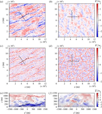
In order to characterize how LSMs in the CBL modulate small-scale turbulence, it is instructive to first consider how structures in the instantaneous velocity field change with bulk stability. Although qualitative in nature, such visualizations provide rich insights on how the structural attributes of LSMs change with stratification. Figure 2 depicts instantaneous snapshots of the velocity field from a weakly (
 $-z_{i}/L=3.1$
, (a,c,e)) and a highly (
 $-z_{i}/L=1082$
, (b,d,f)) convective CBL simulation on the
 $256^{3}$
grid. Snapshots of the instantaneous streamwise velocity
 $\widetilde{u}^{\prime }/w_{\star }$
are displayed in the
 $x$
–
 $y$
plane in figure 2(a) and (b) and the instantaneous vertical velocity is displayed in figure 2(c) and (d), both plotted for
 $z/z_{i}=0.1$
. The elevation of the
 $x$
–
 $y$
slices plotted in figure 2(a–d) is denoted by a horizontal grey line in (e,f). In (e,f), the streamwise velocity is plotted in the
 $x^{\prime }$
–
 $z$
plane, where the
 $x^{\prime }$
–
 $y^{\prime }$
axis can be found overlaid on (a–d). The local
 $x^{\prime }$
–
 $y^{\prime }$
coordinate system is added to highlight an LSM, which is rotated counterclockwise relative to the
 $x$
-axis by virtue of the Coriolis force.
Instantaneous velocity field from
 $256^{3}$
simulations. Results are plotted for a weakly convective CBL (
 $-z_{i}/L=3.1$
) in (a,c,e) and a highly convective CBL (
 $-z_{i}/L=1082$
) in (b,d,f). In (a,b), instantaneous streamwise velocity (
 $\widetilde{u}^{\prime }/w_{\star }$
) is displayed in the
 $x$
–
 $y$
plane, for
 $z/z_{i}=0.10$
. In (c,d), instantaneous vertical velocity (
 $\widetilde{w}^{\prime }/w_{\star }$
) is displayed in the
 $x$
–
 $y$
plane, for
 $z/z_{i}=0.10$
(where the
 $x^{\prime }$
–
 $y^{\prime }$
coordinate system is displayed in (a–d)). In (e,f) instantaneous streamwise velocity is displayed in the
 $x^{\prime }$
–
 $z$
plane with instantaneous
 $u$
–
 $w$
velocity vectors overlaid. The grey horizontal lines in (e,f) denote
 $z/z_{i}=0.10$
, and the solid black lines in (e) denote the structure inclination angle
 $\unicode[STIX]{x1D6FE}=17.7^{\circ }$
.

One can see that for weakly convective conditions, the streamwise velocity field in figure 2(a) is organized into high- and low-momentum streaks, which are typically aligned
 $10^{\circ }$
–
 $20^{\circ }$
to the left of the geostrophic wind in the Northern Hemisphere (LeMone Reference LeMone1973; Brown Reference Brown1980). Corresponding updrafts and downdrafts in the vertical velocity field, sometimes termed horizontal convective rolls (or HCRs) are visible in figure 2(c). In figure 2(e), we display the streamwise velocity (here the velocity component aligned with the roll axis) in the
 $x^{\prime }$
–
 $z$
plane, where the
 $x^{\prime }$
–
 $y^{\prime }$
axis is rotated
 $32^{\circ }$
counterclockwise from the
 $x$
–
 $y$
axis. Also displayed in (e) are inclined lines that indicate the characteristic inclination angle of surface-layer structures,
 $\unicode[STIX]{x1D6FE}=17.7^{\circ }$
, as calculated from the two-point correlation of streamwise velocity
 $R_{uu}(\unicode[STIX]{x0394}x,\unicode[STIX]{x0394}z)$
(discussed below in § 3.4). In (e), a low-momentum region in the streamwise velocity field is evident; ejections of low-momentum fluid occur in this region (as can be seen from the velocity vectors overlaid on the plot). Under weakly convective conditions the organization of the atmospheric surface layer is similar to what is found in the logarithmic region of a canonical wall-bounded turbulent shear flow, except that the low-momentum zones are rotated counterclockwise relative to the geostrophic wind and warm (
 $\unicode[STIX]{x1D703}^{\prime }>0$
) fluid concentrates in the low momentum zones (e.g. see figure 4 of Salesky et al. (Reference Salesky, Chamecki and Bou-Zeid2017)).
Under highly convective conditions (
 $-z_{i}/L=1082$
, (b,d,f)), the CBL exhibits significantly different organization. Here the vertical velocity field organizes into open cells (similar to turbulent Rayleigh–Bénard convection), as can be seen in figure 2(d). The horizontal velocity field in figure 2(b) is comprised of ‘patches’ of high- and low-momentum fluid due to convergence and divergence into updrafts and downdrafts. In contrast to the slightly inclined surface-layer structures seen for weakly convective conditions in figure 2(e), here the structures are much more inclined (indeed, nearly vertical) since the vertical velocity field is dominated by updrafts and downdrafts. Thus as the CBL becomes increasingly convective, the vertical velocity field transitions from horizontal convective rolls to open cells (see Salesky et al.
Reference Salesky, Chamecki and Bou-Zeid2017, for a further discussion). With this, the VLSMs in the streamwise velocity field vanish and are replaced with high- and low-momentum patches, and the inclination angle of surface-layer structures increases from the
 ${\sim}15^{\circ }$
found in neutrally stratified wall turbulence to nearly vertical (Hommema & Adrian Reference Hommema and Adrian2003; Carper & Porté-Agel Reference Carper and Porté-Agel2004; Chauhan et al.
Reference Chauhan, Hutchins, Monty and Marusic2013). Nonetheless, the concept that the large-scale flow is composed of ‘building block’ structures persists across stability regimes. At the near-neutral and near-free convective limits, these ‘building blocks’ resemble LSMs, and convective cells, respectively. In this sense, one may expect that a large-scale amplitude modulation should be preserved across stability regimes, but that the identity of the modulator will transition from the large-scale streamwise velocity
 $u_{l}$
to the large-scale vertical velocity
 $w_{l}$
. Spectrograms are convenient for describing the distribution of spectral density across wavelength and depth, and the following section demonstrates how the flow attains a vertically dominant state at the near-free convection limit.
3.3 Spectrograms
Previous studies of amplitude modulation in turbulent boundary layers (e.g. Kim & Adrian Reference Kim and Adrian1999; Hutchins & Marusic Reference Hutchins and Marusic2007a
,Reference Hutchins and Marusic
b
; Mathis et al.
Reference Mathis, Hutchins and Marusic2009a
,Reference Mathis, Monty, Hutchins and Marusic
b
; Anderson Reference Anderson2016) have found that spectrograms (premultiplied power spectra plotted as a function of dimensionless wavelength and wall-normal distance) provide evidence of very-large-scale motions if an outer peak exists at large wavelengths. In figure 3, we present spectrograms from selected
 $256^{3}$
simulations for weakly (
 $-z_{i}/L=3.1$
(a,d,g)), moderately (
 $-z_{i}/L=17.7$
(b,d,h)) and highly (
 $-z_{i}/L=1082$
(c,f,i)) convective conditions, for the streamwise velocity (
 $k_{x}\unicode[STIX]{x1D6F7}_{uu}/w_{\star }^{2}$
(a,b,c)), vertical velocity (
 $k_{x}\unicode[STIX]{x1D6F7}_{ww}/w_{\star }^{2}$
(d,e,f)) and for the vertical heat flux (
 $k_{x}\unicode[STIX]{x1D6F7}_{w\unicode[STIX]{x1D703}}/w_{\star }\unicode[STIX]{x1D703}_{\star }$
(g,h,i)). To these figures, we have added horizontal and vertical lines to denote the AM filter scale (§ 1.2) and Obukhov length,
 $-L/z_{i}$
, respectively.
Premultiplied spectrograms, plotted as a function of dimensionless wavelength and height from
 $256^{3}$
simulations. Panels (a,d,g) are plotted for
 $-z_{i}/L=3.1$
, (b,e,h) are plotted for
 $-z_{i}/L=17.7$
and (c,f,i) are plotted for
 $-z_{i}/L=1082$
. Spectrograms of streamwise velocity (
 $k_{x}\unicode[STIX]{x1D6F7}_{uu}/w_{\star }^{2}$
) are displayed in (a–c), spectrograms of vertical velocity (
 $k_{x}\unicode[STIX]{x1D6F7}_{ww}/w_{\star }^{2}$
) are displayed in (d–f) and spectrograms of vertical heat flux (
 $k_{x}\unicode[STIX]{x1D6F7}_{w\unicode[STIX]{x1D703}}/w_{\star }\unicode[STIX]{x1D703}_{\star }$
) are displayed in (g–i). In each panel, the horizontal dashed line denotes the cutoff wavelength used to separate the small scales from the large scales (
 $\unicode[STIX]{x1D706}_{x}=z_{i}$
) and the vertical dashed line denotes the normalized Obukhov length (i.e.
 $-L/z_{i}$
).

The spectrogram of streamwise velocity under weakly convective conditions in figure 3(a) exhibits both an inner peak and an outer peak, similar to what has been found in high Reynolds number turbulent boundary layers in the absence of buoyancy. Here the outer peak occurs at
 $z/z_{i}\approx 0.1$
and
 $\unicode[STIX]{x1D706}_{x}/z_{i}\approx 6$
, and may be interpreted as the signature of VLSMs in the streamwise velocity field under weakly convective conditions. The outer peak in this case is smaller than the typically reported value of
 $\unicode[STIX]{x1D706}_{x}/z_{i}\approx 10$
in flows where buoyancy is absent (e.g. Marusic et al.
Reference Marusic, McKeon, Monkewitz, Nagib, Smits and Sreenivasan2010b
); this occurs due to the combined effects of buoyancy and Coriolis. Recall that figure 2(a,c) showed that structures undergo a rotation due to Coriolis, but for the purpose of figure 3, the flow field is projected onto a spectrum of harmonic functions in
 $x$
. This likely manifests in the spectrograms as an existential shortening of the structures at weakly convective cases. Nonetheless, we will show that the outer peak location shifts monotonically, and for increasingly unstable conditions the influence of this post-processing step diminishes since the flow attains a cell-like structure (figure 2
b,d). Other studies of neutrally stratified, Coriolis-free ABL turbulence (Fang & Porté-Agel Reference Fang and Porté-Agel2015; Jacob & Anderson Reference Jacob and Anderson2017) report VLSMs with longer streamwise extent (
 ${\sim}20z_{i}$
), and there is no need to repeat these cases in the present work.
As
 $-z_{i}/L$
increases, one can see (e.g. in figure 3
b) that the outer peak shifts to smaller wavelengths, until only a single peak is found under highly convective conditions in (c). These changes in the spectrograms correspond to the high- and low-momentum streaks in the
 $\tilde{u} ^{\prime }$
field transitioning to patches of high and low momentum fluid due to horizontal convergence and divergence from updrafts and downdrafts in the vertical velocity field (see figure 2
a,b).
Spectrograms of the vertical velocity
 $k_{x}\unicode[STIX]{x1D6F7}_{ww}/w_{\star }^{2}$
are plotted in figure 3(d–f). For weakly convective conditions in (d), the spectrogram of vertical velocity also exhibits an inner peak and an outer peak, with the outer peak found at
 $\unicode[STIX]{x1D706}_{x}/z_{i}\approx 6$
and
 $z/z_{i}\approx 0.5$
. Here the outer peak corresponds to horizontal convective rolls that occur in the
 $\widetilde{w}^{\prime }$
field (see figure 2
c). In contrast to the outer peak for streamwise velocity, which was found in the shear-dominated region of the CBL,
 $z<-L$
, the outer peak for vertical velocity is found in the buoyancy-dominated region, i.e.
 $z>-L$
. As the CBL becomes increasingly convective, the outer peak for
 $\widetilde{w}^{\prime }$
shifts inward, until a single maximum is found near
 $z/z_{i}\approx 0.3$
and
 $\unicode[STIX]{x1D706}_{x}/z_{i}\approx 1$
. Note that the height at which the outer peak occurs is consistent with the maximum in
 $\unicode[STIX]{x1D70E}_{w}^{2}/w_{\star }^{2}$
at each stability, as can be seen in figure 1(e). And although the outer peaks for
 $k_{x}\unicode[STIX]{x1D6F7}_{uu}/w_{\star }^{2}$
and
 $k_{x}\unicode[STIX]{x1D6F7}_{ww}/w_{\star }^{2}$
occur at different heights, they do occur at approximately the same wavelength at each stability.
A similar set of plots for the heat flux
 $k_{x}\unicode[STIX]{x1D6F7}_{w\unicode[STIX]{x1D703}}/w_{\star }\unicode[STIX]{x1D703}_{\star }$
can be found in figure 3(g–i). Once again, an outer peak is found under weakly convective conditions (g) and then shifts inward to smaller wavelengths as
 $-z_{i}/L$
increases. Spectrograms for the intermediate cases (see tables 1 and 2) varied monotonically between the cases shown in figure 3 and are not displayed here for the sake of brevity. The implications of these changes in the spectral properties of the CBL with increasing
 $-z_{i}/L$
for flow modulation phenomena will be discussed further in § 3.5.
Properties of large eddy simulations on
 $256^{3}$
grid, including geostrophic velocity (
 $U_{g}$
), kinematic surface heat flux (
 $Q_{0}$
), convective boundary-layer depth (
 $z_{i}$
), Obukhov length (
 $L$
), bulk stability parameter (
 $-z_{i}/L$
), friction velocity (
 $u_{\unicode[STIX]{x1D70F}}$
) and Deardorff convective velocity scale (
 $w_{\star }$
).

Properties of large eddy simulations on
 $160^{3}$
grid, including geostrophic velocity (
 $U_{g}$
), kinematic surface heat flux (
 $Q_{0}$
), convective boundary-layer depth (
 $z_{i}$
), Obukhov length (
 $L$
), bulk stability parameter (
 $-z_{i}/L$
), friction velocity (
 $u_{\unicode[STIX]{x1D70F}}$
), Deardorff convective velocity scale (
 $w_{\star }$
) and number of ensemble members (
 $N_{e}$
).

3.4 Two-point correlations and inclination angles
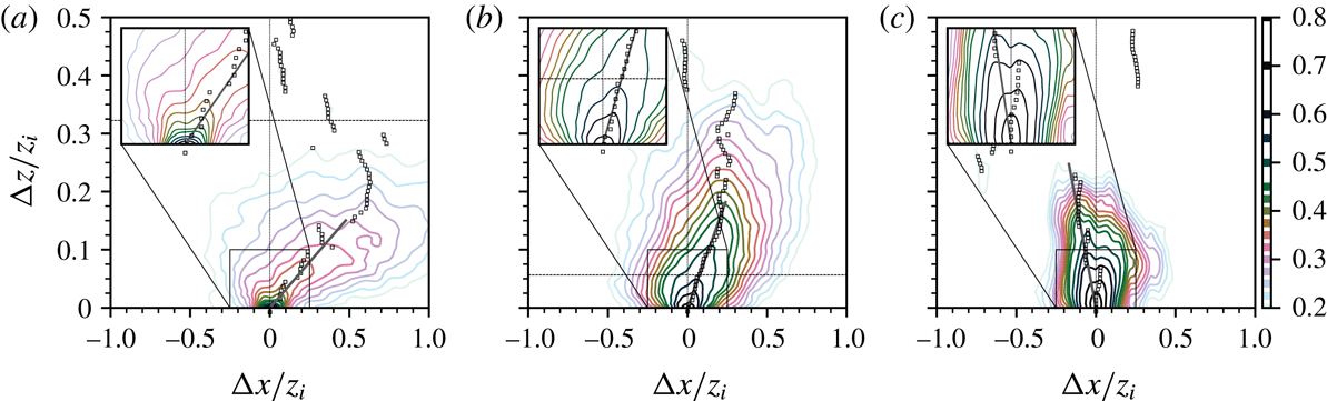
In order to quantify changes in turbulence spatial structure with increasing instability, we here consider the correlation structure of the resolved streamwise velocity field and structure inclination angles. Two-point correlation maps of streamwise velocity are displayed in figure 4(a–c) for weakly, moderately, and highly convective conditions, respectively (for consistency, the selected stratification values are identical to those selected for figure 3). Here the two-point correlation of streamwise velocity is calculated via
 $$\begin{eqnarray}R_{uu}(\unicode[STIX]{x0394}x,\unicode[STIX]{x0394}z)=\frac{\langle \widetilde{u}^{\prime }(x,y,z)\widetilde{u}^{\prime }(x+\unicode[STIX]{x0394}x,y,z+\unicode[STIX]{x0394}z)\rangle }{\unicode[STIX]{x1D70E}_{\widetilde{u}(x,y,z)}\unicode[STIX]{x1D70E}_{\widetilde{u}(x+\unicode[STIX]{x0394}x,y,z+\unicode[STIX]{x0394}z)}},\end{eqnarray}$$
(e.g. Chauhan et al.
Reference Chauhan, Hutchins, Monty and Marusic2013). Taylor’s hypothesis is used to convert a temporal lag to a spatial lag, e.g.
 $\unicode[STIX]{x0394}x=U_{c}\,\unicode[STIX]{x0394}t$
, where the convection velocity
 $U_{c}$
is taken as the mean velocity at
 $z/z_{i}=0.2$
. Other values of the convection velocity were also considered in the computation of
 $R_{uu}$
; we found that this had negligible impact on the resulting inclination angles. This same convection velocity will be used in the computation of two-point amplitude modulation coefficients below. Recall, too, from § 1.2 and (1.8)–(1.9), that we use a local coordinate system mapped to the mean flow direction at each elevation, and thus the reported correlation and inclination angles are true indicators of LSMs. That is, the reported statistics are not artificially shortened by virtue of a Cartesian coordinate system that is oblique to the actual streamwise flow direction.
Two-point correlation maps,
 $R_{uu}$
, plotted as a function of streamwise (
 $\unicode[STIX]{x0394}x/z_{i}$
) and vertical (
 $\unicode[STIX]{x0394}z/z_{i}$
) lags from
 $256^{3}$
simulations. In each panel, the black squares indicate the value of
 $\unicode[STIX]{x0394}x/z_{i}$
that corresponds to the maximum correlation for each value of
 $\unicode[STIX]{x0394}z/z_{i}$
. Solid lines are fit by linear regression to the maximum correlation for points in the range
 $\unicode[STIX]{x0394}z/z_{i}\in [0,0.2]$
and are used to calculate the inclination angle of the surface-layer structures. The horizontal dashed line in each plot indicates the location of the Obukhov length, i.e.
 $-L/z_{i}$
. (a)
 $-z_{i}/L=3.1$
, (b)
 $-z_{i}/L=17.7$
, (c)
 $-z_{i}/L=1082$
.

Inclination angle (
 $\unicode[STIX]{x1D6FE}$
) of surface-layer structures calculated from
 $160^{3}$
and
 $256^{3}$
LES results, plotted as a function of Monin–Obukhov stability parameter
 $-\unicode[STIX]{x1D701}$
. The fit proposed by Chauhan et al. (Reference Chauhan, Hutchins, Monty and Marusic2013) is shown for comparison (solid line); dashed lines indicate
 $\pm 5^{\circ }$
from this empirical curve. Also displayed are values of
 $\unicode[STIX]{x1D6FE}$
calculated from unstable atmospheric surface-layer data from Carper & Porté-Agel (Reference Carper and Porté-Agel2004), Marusic & Heuer (Reference Marusic and Heuer2007) and Chauhan et al. (Reference Chauhan, Hutchins, Monty and Marusic2013).

In figure 4, contours of
 $R_{uu}$
are plotted as a function of the normalized horizontal and vertical lag; the black squares denote the streamwise lag that corresponds to the maximum correlation (i.e.
 $\unicode[STIX]{x0394}x^{\ast }$
) for each vertical lag. In order to determine the characteristic inclination of surface-layer structures at each stability, we perform a linear regression of the form
 $\unicode[STIX]{x0394}z=c_{1}\unicode[STIX]{x0394}x^{\ast }$
for
 $\unicode[STIX]{x0394}z/z_{i}\in [0,0.2]$
to determine the unknown coefficient
 $c_{1}$
. The inclination angle is then given as
 $\unicode[STIX]{x1D6FE}=\tan ^{-1}(c_{1})$
. In figure 4, one can see that as
 $-z_{i}/L$
increases, the region of maximum correlation goes from being inclined in the
 $+\unicode[STIX]{x0394}x$
direction to nearly aligned with the
 $\unicode[STIX]{x0394}z$
axis, indicating that the steepness of surface layer structures increases with increasing
 $-z_{i}/L$
. This result is thoroughly consistent with the qualitative results displayed in figure 2 and the shift in the outer peak with increasing
 $-z_{i}/L$
that can be seen in figure 3: LSMs steepen and approach the classical convective cells as
 $-z_{i}/L\rightarrow \infty$
.
The change in surface-layer structures with increasing instability can be seen more clearly in figure 5, where the inclination angle
 $\unicode[STIX]{x1D6FE}$
is plotted as a function of the MO stability variable
 $-\unicode[STIX]{x1D701}=-z/L$
, at both grid resolutions. Also displayed in figure 5 is the empirical fit from the atmospheric surface-layer data of Chauhan et al. (Reference Chauhan, Hutchins, Monty and Marusic2013),
 $$\begin{eqnarray}\unicode[STIX]{x1D6FE}=\unicode[STIX]{x1D6FE}_{0}+7.3\ln (1-70\unicode[STIX]{x1D701}),\end{eqnarray}$$
where
 $\unicode[STIX]{x1D6FE}_{0}=12^{\circ }$
, dashed lines indicating
 $\unicode[STIX]{x1D6FE}\pm 5^{\circ }$
from this fit, and data collected under unstable conditions (
 $\unicode[STIX]{x1D701}<0$
) from several experimental studies are superimposed to broaden the context of the results (Carper & Porté-Agel Reference Carper and Porté-Agel2004; Marusic & Heuer Reference Marusic and Heuer2007; Chauhan et al.
Reference Chauhan, Hutchins, Monty and Marusic2013). Here we observe that as
 $-\unicode[STIX]{x1D701}$
increases, the inclination angle increases from
 $10^{\circ }$
–
 $15^{\circ }$
to more than
 $50^{\circ }$
. While there is some scatter in the values of
 $\unicode[STIX]{x1D6FE}$
calculated from the LES results, the scatter we observe is comparable to what is found in the experimental data. This plot reinforces the conclusion that surface-layer structures become more steeply inclined with increasing instability, which can be interpreted as buoyancy modifying hairpin vortex packets to become lifted up from the ground (e.g. Hommema & Adrian Reference Hommema and Adrian2003). As discussed previously, spectrograms indicate that LSMs persist to highly convective conditions (figure 3
f). As such, we expect that inner-layer modulation by large-scale outer-layer structures should continue with increasing
 $-z_{i}/L$
, as long as there is a separation between the inner and outer peaks.
3.5 Modulation of small scales
Time series depicting modulation of small-scale streamwise velocity by large-scale streamwise velocity and large-scale vertical velocity for
 $-z_{i}/L=3.1$
simulation on
 $160^{3}$
grid at
 $z/z_{i}=0.15$
. (a) Time series of small-scale (
 $u_{s}$
) and large-scale (
 $u_{l}$
) streamwise velocity and large-scale envelope of small-scale streamwise velocity (
 $E_{l}(u_{s})$
), (b) time series of small-scale (
 $w_{s}$
) and large-scale (
 $w_{l}$
) vertical velocity, (c) time series of the filtered envelope (
 $E_{l}(u_{s})$
) of small-scale velocity with large-scale streamwise and vertical velocity also shown for comparison, (d) wavelet power spectra of streamwise velocity normalized by frequency and streamwise velocity variance. Here the dashed horizontal line denotes the cutoff frequency used to separate large from small scales. The amplitude modulation coefficients at this height are
 $R_{u_{l},u_{s}}=-0.60$
and
 $R_{w_{l},u_{s}}=0.62$
.

We now consider the extent to which amplitude modulation occurs in the convective atmospheric boundary layer. Before exploring the dependence of AM on height (
 $z/z_{i}$
) and on stability (
 $-z_{i}/L$
), we first provide an example of the amplitude modulation of small-scale streamwise velocity (
 $u_{s}$
) by both large-scale streamwise (
 $u_{l}$
) and vertical velocity (
 $w_{l}$
). This is done to illustrate the temporal variability of the quantities that enter into the calculation of the AM coefficient in (1.3)–(1.7) (e.g.
 $E_{l}^{\prime }(u_{s})$
, and
 $u_{l}$
or
 $w_{l}$
). In figure 6, we plot time series of streamwise and vertical velocity and wavelet spectra for the
 $-z_{i}/L=3.1$
simulation on the
 $160^{3}$
grid, at
 $z/z_{i}=0.15$
. In figure 6(a), we display time series of the large-scale (
 $u_{l}$
) and small-scale (
 $u_{s}$
) streamwise velocity components as well as the large-scale envelope of the small-scale streamwise velocity
 $E_{l}(u_{s})$
. The corresponding large- and small-scale components of vertical velocity are shown in (b). In (c),
 $u_{l}$
,
 $w_{l}$
and
 $E_{l}^{\prime }(u_{s})$
are included on the same plot, so one can see visual evidence of the correlation between the large-scale velocity components and the large-scale envelope of
 $u_{s}$
. Finally in (d), we display wavelet power spectra of the streamwise velocity, plotted as a function of large eddy turnover time. The wavelet power spectrum is computed by first calculating the wavelet transform of the streamwise velocity
 $u$
, defined via convolution with a spectrum of wavelet functions:
 $$\begin{eqnarray}\widehat{u}(z;t_{s},t)=\int u(z,t^{\prime })\,\unicode[STIX]{x1D713}^{\ast }\left(\frac{t^{\prime }-t}{t_{s}}\right)\text{d}t^{\prime },\end{eqnarray}$$
where
 $\unicode[STIX]{x1D713}(t_{s},t)$
is the wavelet function with characteristic time scale,
 $t_{s}$
, and
 $(\cdot )^{\ast }$
denotes the complex conjugate. We employ the Morlet wavelet
 $$\begin{eqnarray}\unicode[STIX]{x1D713}(t/t_{s})=\text{e}^{\text{i}\unicode[STIX]{x1D714}_{\unicode[STIX]{x1D713}}t/t_{s}}\text{e}^{-|t/t_{s}|^{2}/2},\end{eqnarray}$$
for its high-frequency resolution where the complex frequency
 $|\unicode[STIX]{x1D714}_{\unicode[STIX]{x1D713}}|=6$
(Baars et al.
Reference Baars, Talluru, Hutchins and Marusic2015). Given the complex wavelet coefficients, one can then calculate the wavelet power spectrum:
 $$\begin{eqnarray}E_{u}(z;t_{s},t)=\frac{|\widehat{u}(z;t_{s},t)|^{2}}{t_{s}}.\end{eqnarray}$$
In figure 6(c) there is visual evidence of a negative correlation between large-scale streamwise velocity
 $u_{l}$
and the filtered envelope of small-scale
 $u$
(
 $E_{l}^{\prime }(u_{s})$
). Here the envelope of
 $u_{s}$
increases due to modulation by a low-momentum LSM (i.e.
 $u_{l}<0$
) and decreases due to modulation by a high-momentum LSM (
 $u_{l}>0$
). This is consistent with previous studies of amplitude modulation in turbulent boundary layers in the absence of buoyancy (e.g. Mathis et al.
Reference Mathis, Hutchins and Marusic2009a
,Reference Mathis, Monty, Hutchins and Marusic
b
; Marusic et al.
Reference Marusic, Mathis and Hutchins2010a
). At this height, the single-point amplitude modulation coefficient is
 $R_{u_{l},u_{s}}=-0.60$
. From figure 6(b,c), one can see that AM due to large-scale vertical velocity also occurs, but here amplitude modulation is positive (
 $R_{w_{l},u_{s}}=0.62$
). We observe that small-scale streamwise velocity fluctuations are excited in large-scale updraft regions (
 $w_{l}>0$
) and suppressed in large-scale downdraft regions (
 $w_{l}<0$
), due to the positive correlation between
 $w_{l}$
and the envelope of the small-scale velocity fluctuations (
 $E_{l}(u_{s})$
). It is also interesting to consider how the energy content in
 $u$
varies as a function of frequency and time relative to
 $u_{l}$
and
 $w_{l}$
. One can see from figure 6(c,d) that regions of
 $w_{l}>0$
and
 $u_{l}<0$
correspond to a shift of energy in
 $E_{u}$
to higher frequencies (see, e.g.
 $tw_{\star }/z_{i}=4$
, 13–14, 16), reinforcing the picture that these large-scale structures modulate small-scale turbulence. As noted in § 1.2, the horizontal velocity components have been mapped to the local mean flow direction at each elevation, and thus the physics associated with the passage of LSMs are accurately captured (for high Rossby number cases, the local mean flow would be precisely aligned with the
 $x$
axis).
Next, we turn our attention to how both single- and two-point amplitude modulation coefficients depend on height (
 $z/z_{i}$
) and on atmospheric stability (
 $-z_{i}/L$
). Profiles of the single- and two-point AM coefficients of
 $u_{s}$
(a,b),
 $w_{s}$
(c,d) and
 $\unicode[STIX]{x1D703}_{s}$
(e,f), and surface fluxes
 $(u\,w)_{s}$
(g,h), and
 $(w\,\unicode[STIX]{x1D703})_{s}$
(i,j), can be found in figure 7, due to modulation by large-scale
 $u$
(a,c,e,g,i)
 $w$
(b,d,f,h,j). In each panel solid lines are used to indicate single-point AM coefficients, and dashed lines are used to indicate two-point AM coefficients, where the reference height used to calculate the two-point coefficients,
 $z_{ref}/z_{i}=0.2$
, is indicated by the vertical grey line.
Single-point (solid lines) and two-point (dashed lines) amplitude modulation coefficients from
 $160^{3}$
simulations. The vertical grey line in each panel denotes the reference height (
 $z_{ref}/z_{i}=0.2$
) used when calculating the two-point coefficients. Panels (a,c,e,g,i) denote amplitude modulation by large-scale streamwise velocity (
 $u_{l}$
) and panels (b,d,f,h,j) denote modulation by large-scale vertical velocity (
 $w_{l}$
). (a,b) Modulation of small-scale streamwise velocity (
 $u_{s}$
), (c,d) modulation of small-scale vertical velocity (
 $w_{s}$
), (e,f) modulation of small-scale temperature (
 $\unicode[STIX]{x1D703}_{s}$
), (g,h) modulation of small-scale momentum flux (
 $uw_{s}$
), (i,j) modulation of small-scale heat flux (
 $w\unicode[STIX]{x1D703}_{s}$
). In (a), black diamonds denote
 $R_{u_{l},u_{s}}$
from smooth-wall channel flow data (taken from Mathis et al.
Reference Mathis, Monty, Hutchins and Marusic2009b
, their figure 3a).

In figure 7(a), modulation of small-scale
 $u$
by large-scale
 $u$
, i.e.
 $R_{u_{l},u_{s}}$
, is displayed for the suite of simulations on the
 $160^{3}$
grid. The smooth-wall channel flow data of Mathis et al. (Reference Mathis, Monty, Hutchins and Marusic2009b
) are also included in this panel for comparison. One can see from this panel that the single-point AM coefficient attains positive values close to the ground, and changes sign between
 $z/z_{i}=0.05$
–0.1, depending on the stability. As
 $-z_{i}/L$
increases, the magnitude of the single-point AM coefficient decreases, until the modulation is negligible. Note that the most highly convective case (
 $-z_{i}/L=1041$
) has been omitted from these plots because the AM profiles are extremely noisy; this appears to occur because there is no separation between the outer and inner peak and the concept of amplitude modulation is no longer meaningful in this case.
The behaviour of the two-point AM coefficients, indicated by the dashed lines, is similar, except that (as expected) the two-point coefficients attain smaller values farther from the reference height. These results indicate that as the outer peak in the spectrogram of
 $u$
shifts to smaller wavelengths, the scale separation between the outer peak and inner peak decreases, such that the amplitude modulation of small-scale turbulence is significantly reduced. Thus one can conclude that amplitude modulation due to
 $u_{l}$
is a significant dynamical feature of weakly convective CBLs, where VLSMs exist in the streamwise velocity field. However, as
 $-z_{i}/L$
increases, surface-layer structures become shorter and more inclined, and amplitude modulation due to
 $u_{l}$
becomes negligible.
Depth-integrated single- (a,b) and two-point (c,d) AM coefficients by large-scale streamwise (a,c) and vertical (b,d) velocity. Integrals are shown on the ordinate and correlations are denoted on the abscissa, where the panel (a) inset denotes the colour scheme (for clarity, the colour scheme is identical to that of figure 7). Panel (a) includes the depth-integrated integral of the Mathis et al. (Reference Mathis, Monty, Hutchins and Marusic2009b ) data points.

Profiles of AM coefficients where modulation by large-scale vertical velocity is considered are given in figure 7(b,d,f,h,j). In contrast to modulation by large-scale
 $u$
, amplitude modulation due to
 $w_{l}$
is positive throughout much of the depth of the CBL, the magnitude of
 $R$
is larger for most quantities, and
 $R$
remains large as
 $-z_{i}/L$
increases. Physically, this means that amplitude modulation by large-scale
 $w$
occurs both under weakly convective conditions, where the updrafts are organized into long, linear features (HCRs) and under highly convective conditions, where buoyant plumes occur and the
 $w$
field organizes into open cells on large scales. As discussed above, the physical interpretation is that small-scale turbulence is excited in updraft regions, and suppressed in downdraft regions. This is conceptually analogous to the intermittent periods of small-scale excitation and quiescence between large-scale low- and high-momentum regions, respectively (Mathis et al.
Reference Mathis, Hutchins and Marusic2011).
In order to summarize the figure 7 result, and to assess the extent to which AM occurs in the CBL in a global sense, we have also plotted depth-averaged values of the AM coefficients, which are shown in figure 8. That is, we plot histograms of the quantity
 $\overline{R}=(1/z_{i})\int _{0}^{z_{i}}R_{b_{l},a_{s}}\,\text{d}z$
, where
 $R_{b_{l},a_{s}}$
is the AM coefficient between the large-scale quantity
 $b_{l}$
and the small-scale quantity
 $a_{s}$
. Note that by definition,
 $\overline{R}\in [-1,1]$
since
 $R_{b_{l},a_{s}}\in [-1,1]$
. This figure helps to better characterize global changes in AM with
 $-z_{i}/L$
, since discerning differences in the figure 7 was difficult in some cases. Figure 8(a,c) and (b,d) shows modulation of small-scale amplitude by
 $u_{l}$
and
 $w_{l}$
, respectively; where values of
 $\overline{R}$
calculated from the single-point AM coefficient are displayed in (a,b) and values calculated from the two-point AM coefficient are displayed in (c,d). Perhaps the most striking result can be seen in the single-point correlations of
 $u_{l}$
with small-scale quantities in (a), where
 $|\overline{R}|$
is the largest for weakly convective (e.g.
 $-z_{i}/L=3.1$
) conditions and AM becomes negligible (
 $\overline{R}\approx 0$
) as
 $-z_{i}/L$
increases. This can be seen very clearly for
 $R_{u_{l},u_{s}}$
where the neutral channel flow data (Mathis et al.
Reference Mathis, Monty, Hutchins and Marusic2009b
) are displayed together with the CBL LES results in (a).
In contrast, the average AM coefficients between
 $w_{l}$
and small-scale quantities exhibit very little dependence on
 $-z_{i}/L$
for all quantities considered. This is true for both single (b) and two-point (d) correlations, respectively. This demonstrates that
 $w_{l}$
is a ‘buoyancy proof’ modulator and AM due to
 $w_{l}$
occurs in an global sense as long as sufficient scale separation exists between the inner and outer peaks. It is not surprising that, for near-neutral cases, both
 $u_{l}$
and
 $w_{l}$
modulate small-scale quantities, since
 $u_{l}$
and
 $w_{l}$
are both so inherently tied to the identity of LSMs (where low- and high-momentum regions exhibit
 $\{u_{l}<0,w_{l}>0\}$
and
 $\{u_{l}>0,w_{l}<0\}$
, respectively). As surface heating increases, however, and the flow structure transitions to buoyant plumes (and
 $u^{\prime }$
becomes decorrelated from
 $w^{\prime }$
, e.g. figure 2
b,d), it is entirely reasonable for
 $w_{l}$
to be the only plausible modulator. The correlations demonstrate this, and the results are consistent with all preceding results shown here (figures 2 to 5).
The effects of unstable stratification on LSMs and amplitude modulation are summarized in the conceptual diagram presented in figure 9. A canonical neutrally stratified high-
 $\mathit{Re}$
boundary layer is depicted in figure 9(a), a moderately convective ABL in (b) and a free convective ABL in (c). In (a,b), the surface layer is denoted by the dashed horizontal line. (Note that the diagram is not drawn to scale in order to emphasize AM within the surface layer.) For neutral stratification (a), the inclination angle of the hairpin vortex packet is
 $\unicode[STIX]{x1D6FE}\approx 15^{\circ }$
. In the surface layer (
 $z/z_{i}\lesssim 0.1$
), positive AM of a small-scale signal occurs in regions where
 $u_{l}^{\prime }>0$
and
 $w_{l}^{\prime }<0$
and negative AM occurs where
 $u_{l}^{\prime }<0$
and
 $w_{l}^{\prime }>0$
. As the ABL becomes unstably stratified (b), the inclination angle of surface-layer structures increases and LSMs become shorter than what is found in the neutral case. Once again AM in the surface layer is positive in regions where
 $u_{l}^{\prime }>0$
and
 $w_{l}^{\prime }<0$
and negative in regions where
 $u_{l}^{\prime }<0$
and
 $w_{l}^{\prime }>0$
. Finally, in the free-convective case (c), the LSMs shorten further and the inclination angle of surface-layer structures is
 $\unicode[STIX]{x1D6FE}\approx 90^{\circ }$
. In this case,
 $u_{l}$
is no longer an effective modulator. Near the ground, positive AM does occur in regions where
 $w_{l}^{\prime }<0$
and negative AM occurs in regions where
 $w_{l}^{\prime }>0$
. Here it also should be noted that
 $w_{l}^{\prime }>0$
regions are narrower than the
 $w_{l}^{\prime }<0$
regions, due to the positive skewness of
 $w$
(e.g. figure 1
f).
Conceptual diagram depicting the effects of buoyancy on LSMs and amplitude modulation in boundary layers with unstable thermal stratification. (a) Neutral case (canonical high-
 $\mathit{Re}$
boundary layer). (b) Shear–buoyancy transition where
 $U_{g}\neq 0$
and
 $Q_{0}>0$
. (c) Free convection where
 $U_{g}=0$
and
 $Q_{0}$
is finite. The figure is not drawn to scale in order to emphasize amplitude modulation within the surface layer (denoted by the horizontal dashed line). Note that
 $x^{\prime }$
denotes the direction aligned with the axis of the LSMs.

Finally, we emphasize that the strongest correlation is found between
 $w_{l}$
and small-scale momentum fluxes,
 $(uw)_{s}$
. Since
 $(uw)_{s}=u_{\unicode[STIX]{x1D70F}}^{2}$
at the wall, this result may have implications for development of surface flux models for use in wall-modelled LES (Pope Reference Pope2000; Marusic et al.
Reference Marusic, McKeon, Monkewitz, Nagib, Smits and Sreenivasan2010b
).
4 Discussion and conclusions
Previous studies in high-
 $\mathit{Re}$
wall-bounded turbulent shear flows (e.g. Kovasznay et al.
Reference Kovasznay, Kibens and Blackwelder1970; Brown & Thomas Reference Brown and Thomas1977; Nakagawa & Nezu Reference Nakagawa and Nezu1981; Murlis et al.
Reference Murlis, Tsai and Bradshaw1982; McLean Reference McLean1990; Wark & Nagib Reference Wark and Nagib1991; Adrian et al.
Reference Adrian, Meinhart and Tomkins2000; Ganapathisubramani et al.
Reference Ganapathisubramani, Longmire and Marusic2003; Tomkins & Adrian Reference Tomkins and Adrian2003; Del Alamo et al.
Reference Del Alamo, Jiménez, Zandonade and Moser2004; Guala et al.
Reference Guala, Hommema and Adrian2006; Hambleton et al.
Reference Hambleton, Hutchins and Marusic2006; Hutchins & Marusic Reference Hutchins and Marusic2007b
,Reference Hutchins and Marusic
a
; Chung & McKeon Reference Chung and McKeon2010; Lee & Sung Reference Lee and Sung2011; Wu et al.
Reference Wu, Baltzer and Adrian2012) have revealed the existence of so-called large-scale and very-large-scale motions, regions of high- and low-momentum fluid elongated in the streamwise direction that populate the logarithmic layer and modulate the amplitude of small-scale turbulent fluctuations (Mathis et al.
Reference Mathis, Hutchins and Marusic2009a
,Reference Mathis, Monty, Hutchins and Marusic
b
; Marusic et al.
Reference Marusic, Mathis and Hutchins2010a
). Using a suite of large eddy simulations of canonical dry, barotropic CBLs at mid-latitudes spanning weakly to highly convective conditions, we have investigated the extent to which these coherent structures are modified by unstable stratification and how, in turn, these structures influence amplitude modulation phenomena in the convective atmospheric boundary layer. The main conclusions of this study are outlined below:
(i) The topology of turbulent coherent structures changes dramatically as the CBL becomes increasingly unstable. Under weakly convective conditions (small
 $-z_{i}/L$
), VLSMs occur in the streamwise velocity field, similar to what is found in turbulent boundary layers in the absence of buoyancy. As
$-z_{i}/L$
increases, the streamwise velocity field transitions to patches of high- and low-momentum fluid. Concurrent changes occur in the large-scale vertical velocity field, from horizontal convective rolls under weakly convective conditions to open cells under highly convective conditions (see Salesky et al. (Reference Salesky, Chamecki and Bou-Zeid2017) for a further discussion on the roll to cell transition). In addition, the inclination angle of hairpin vortex packets (as deduced from the two-point correlation of
$u$
) in the atmospheric surface layer increases, from
$\unicode[STIX]{x1D6FE}\approx 15^{\circ }$
for near-neutral conditions to nearly vertical under highly convective conditions. This is consistent with the picture of hairpin vortex packets being lifted up away from the wall due to buoyancy effects (Hommema & Adrian Reference Hommema and Adrian2003).
(ii) Under weakly convective conditions, a distinct inner and outer peak can be seen in the premultiplied spectrogram of
$u$
, with the outer peak located near
$\unicode[STIX]{x1D706}_{x}/z_{i}\approx 6$
, providing spectral evidence of the existence of VLSMs. This value is smaller than the
$\unicode[STIX]{x1D706}_{x}\approx 20z_{i}$
reported in neutrally stratified wall turbulence due to the combined effects of unstable stratification and rotation in the convective boundary layer. As
$-z_{i}/L$
increases, the outer peak shifts to smaller wavelengths and lower heights, until only a single peak is found at
$\unicode[STIX]{x1D706}_{x}/z_{i}\approx 1$
under highly convective conditions (i.e. the VLSMs are replaced by LSMs). A similar feature can be observed in the spectrograms of
$w$
, where an inner and an outer peak both occur for weakly convective conditions (with the outer peak of
$w$
located at
$\unicode[STIX]{x1D706}_{x}/z_{i}\approx 6$
), but the two peaks shift together and eventually merge under highly convective conditions such that the peak in energy is concentrated at a single wavelength (
$\unicode[STIX]{x1D706}_{x}/z_{i}\approx 1$
) and height (
$z/z_{i}\approx 0.3$
).(iii) The extent to which amplitude modulation of small-scale turbulence is modified by buoyancy was investigated using the decoupling procedure proposed by Mathis et al. (Reference Mathis, Hutchins and Marusic2009a ). Under weakly convective conditions, significant amplitude modulation of small-scale fluctuating velocity, temperature and instantaneous second-order moments occurs both due to large-scale streamwise velocity
$u_{l}$
and large-scale vertical velocity
$w_{l}$
. As
$-z_{i}/L$
increases and the separation between the inner and outer peak in the
$u$
spectrum decreases, the degree of amplitude modulation due to
$u_{l}$
also decreases until it is negligible. However, amplitude modulation due to
$w_{l}$
was found to be significant for all stabilities considered, as long as there was a sufficient separation between the inner and outer peak.


It should be noted that amplitude modulation due to large-scale vertical velocity in the CBL has been observed previously from the aircraft data of LeMone (Reference LeMone1976), in the horizontal convective roll regime (see her figure 2). In particular, she found that the magnitude of fluctuations in
 $u^{\prime }$
,
 $v^{\prime }$
,
 $w^{\prime }$
,
 $\unicode[STIX]{x1D703}^{\prime }$
, and absolute humidity
 $\unicode[STIX]{x1D70C}_{v}^{\prime }$
as well as instantaneous fluxes (
 $u^{\prime }w^{\prime }$
,
 $v^{\prime }w^{\prime }$
,
 $w^{\prime }\unicode[STIX]{x1D703}^{\prime }$
and
 $\unicode[STIX]{x1D70C}_{v}^{\prime }w^{\prime }$
) increased dramatically when the ‘roll-scale’ vertical velocity
 $w_{l}$
was positive. Other studies (Weckwerth, Wilson & Wakimoto Reference Weckwerth, Wilson and Wakimoto1996) have highlighted the fact that the modulation of small-scale turbulent fluctuations in HCR updraft regions can lead to coherent perturbations of scalar quantities such as potential temperature and water vapour mixing ratio, and play a significant role for the initiation of deep, moist convection. Our results are consistent with these previous studies conducted in the atmospheric boundary layer as well as with flow modulation phenomena that have been observed in neutrally stratified turbulent shear flows (e.g. Mathis et al.
Reference Mathis, Hutchins and Marusic2009a
,Reference Mathis, Monty, Hutchins and Marusic
b
; Marusic et al.
Reference Marusic, Mathis and Hutchins2010a
).
Finally, it is appropriate to discuss our present results in the context of Monin–Obukhov (MO) similarity theory, long considered to be the cornerstone of atmospheric boundary-layer studies. In spite of its remarkable success (Businger et al.
Reference Businger, Wyngaard, Izumi and Bradley1971; Kaimal et al.
Reference Kaimal, Wyngaard, Izumi and Coté1972; Högström Reference Högström1988; Kaimal & Finnigan Reference Kaimal and Finnigan1994), deviations from MO similarity are well documented in the literature (Kaimal et al.
Reference Kaimal, Wyngaard, Izumi and Coté1972; Panofsky et al.
Reference Panofsky, Tennekes, Lenschow and Wyngaard1977; Khanna & Brasseur Reference Khanna and Brasseur1997; Johansson et al.
Reference Johansson, Smedman, Högström, Brasseur and Khanna2001; Salesky & Chamecki Reference Salesky and Chamecki2012), and the potential for generalizations is widely accepted. Two of the key assumptions underlying MO similarity are those of horizontal statistical homogeneity, and the attached eddy hypothesis (Townsend Reference Townsend1976), where the characteristic length scale of turbulent motions is taken to be the distance from the wall
 $z$
. Our present results demonstrate that even in canonical convective atmospheric boundary layers, significant spatial and temporal variability exists in instantaneous small-scale fluctuating quantities due to amplitude modulation by LSMs (that scale on the outer length scale
 $z_{i}$
). That is, surface-layer fluxes undergo a cyclic excitation and relaxation with the passage of LSMs aloft. Thus modulation phenomena are superimposed upon the ‘background values’ of the surface fluxes, thereby inducing significant spatial and temporal variability in the fluxes. Accounting for LSMs and flow modulation phenomena in models of geophysical flows (such as the atmospheric boundary layer) may prove to be a fruitful area of future research.
Acknowledgements
This work was supported by the US Air Force Office of Scientific Research, grant no. FA9550-14-1-0394 (W.A.), and the National Science Foundation, grant no. AGS-1500224 (W.A.). Simulations were run on the Cedar cluster through Compute Canada (www.computecanada.ca).
Appendix
Previous studies have comprehensively demonstrated that amplitude and frequency modulation correlations are invariant to LES grid resolution (Anderson Reference Anderson2016; Awasthi & Anderson Reference Awasthi and Anderson2018). However, these studies have focused on other aspects of inner–outer interactions, and have not considered the dynamics of small-scale modulation in the presently considered low Rossby and Richardson number flow arrangements. We performed additional testing of resolution sensitivity, with results shown in this appendix. Since these results do not contribute to physical insights of structural attributes, etc., we elected to show these results separately from the scientific narrative.
Vertical profiles of amplitude modulation coefficients from relatively high- (
 $160^{3}$
, solid profile) and low-resolution (
 $80^{3}$
, dashed profile) LES. Panels (a,b) denote modulation of small-scale streamwise velocity amplitude by large-scale streamwise (
 $u_{l}$
) and vertical (
 $w_{l}$
) velocity, respectively. Profiles correspond to simulations with identical forcings (
 $U_{g}=15~\text{m}~\text{s}^{-1}$
and
 $Q_{0}=0.07~\text{K}~\text{m}~\text{s}^{-1}$
), where slightly larger values of
 $-z_{i}/L$
are found for simulations on the coarser grid (
 $-z_{i}/L=4.4$
) than for the finer grid (
 $-z_{i}/L=3.1$
).

Figure 10(a,b) shows the single-point AM coefficient denoting modulation of
 $u_{s}$
by
 $u_{l}$
and
 $w_{l}$
, respectively, where the line colours are denoted on (a). The abscissa is log scale, which has the effect of visually amplifying the figure space available to the atmospheric surface layer (i.e.
 $z/z_{i}\lesssim 10^{-1}$
), where resolution differences due to time averaging will be greatest. Nonetheless, in the bulk of the flow, it is clear that the correlations are in close agreement – magnitude and profile.
Figure 10 corresponds with the same forcings (
 $U_{g}=15~\text{m}~\text{s}^{-1}$
and
 $Q_{0}=0.07~\text{K}~\text{m}~\text{s}^{-1}$
) for the simulations on the coarser (
 $80^{3}$
) and finer (
 $160^{3}$
) grid. We observed slightly larger values of
 $-z_{i}/L$
for the
 $80^{3}$
simulation (i.e.
 $-z_{i}/L=4.4$
) than for the
 $160^{3}$
simulation (
 $-z_{i}/L=3.1$
); however, this did not affect the agreement between the AM coefficients at the two resolutions. We considered the AM correlations between
 $u_{l}$
and
 $w_{l}$
and other quantities, at a range of
 $-z_{i}/L$
, and found similar agreement. We elected not to show these results here for brevity. Further evidence that the spatial nature of the flow is captured adequately at the resolution we consider here can be found in figure 5, where the inclination angle of structures is plotted for simulation results on the
 $160^{3}$
and on the
 $256^{3}$
grids.