1. Introduction
Determining the pathways in the ocean that take the large-scale forcing from winds or tides, and convert this to small-scale internal waves and mixing, is one of the fundamental problems of physical oceanography (Wunsch & Ferrari Reference Wunsch and Ferrari2004; Ferrari & Wunsch Reference Ferrari and Wunsch2009). One major puzzle is how energy is transferred from low-mode internal waves such as those generated near topographic features, and converted to higher-mode internal waves, where it is subject to various instabilities and ultimately mixing (Laurent & Garrett Reference Laurent and Garrett2002; Garrett & Kunze Reference Garrett and Kunze2007; Alford et al. Reference Alford and Peacock2015). Higher-mode waves are an energetic component of measurements nearly everywhere in the ocean, yet their existence requires a mechanism to couple such widely separated scales. Nonlinearities in the fluid equations themselves can give rise to instabilities that could potentially do this, but tend to be very weak at large scales (Laurent & Garrett Reference Laurent and Garrett2002).
A different mechanism is the coupling of the fluid with the boundary of its domain. A large body of work has considered how both small-amplitude topography as well as big, steep features on the bottom of the ocean, such as the Hawaiian island chain, the mid-Atlantic ridge, the Luzon Strait or idealized models thereof, can generate low-mode internal waves from the semi-diurnal tide (Bell Reference Bell1975a ; Müller & Xu Reference Müller and Xu1992; Balmforth, Ierley & Young Reference Balmforth, Ierley and Young2002; Llewellyn Smith & Young Reference Llewellyn Smith and Young2002, Reference Llewellyn Smith and Young2003; Khatiwala Reference Khatiwala2003; Nycander Reference Nycander2005; Petrelis, Llewellyn Smith & Young Reference Petrelis, Llewellyn Smith and Young2006; Balmforth & Peacock Reference Balmforth and Peacock2009; Zhao et al. Reference Zhao, Alford, Girton, Johnston and Carter2011). Most of the energy in the low-mode waves propagates away from the generation source (Ray & Mitchum Reference Ray and Mitchum1996; Zhao, Alford & MacKinnon Reference Zhao, Alford and MacKinnon2010), where it encounters other topographic features that can transfer energy to smaller scales. Some of this scattering is due to interactions with the continental slopes (Kelly et al. Reference Kelly, Jones, Nash and Waterhouse2013). Another 1 TW of energy, roughly 25–30 % of the total, is dissipated in the deep ocean (Egbert & Ray Reference Egbert and Ray2000), away from continental slopes and shallow seas.
Several possible topographic mechanisms have been proposed to explain this deep-ocean dissipation. Some studies have considered the effect of isolated features, often modelled as triangular hills or knife-edge ridges, in scattering and dissipating the tides (Müller & Liu Reference Müller and Liu2000; Klymak et al. Reference Klymak, Buijsman, Legg and Pinkel2013; Legg Reference Legg2014). Others have considered the role that rough, small-amplitude topography found in many regions of the ocean basin away from large features could play in scattering energy to higher wavenumbers (Bühler & Holmes-Cerfon Reference Bühler and Holmes-Cerfon2011; Kelly et al. Reference Kelly, Jones, Nash and Waterhouse2013; Li & Mei Reference Li and Mei2014). Mathur, Carter & Peacock (Reference Mathur, Carter and Peacock2014) compared these two mechanisms numerically in a two-dimensional ocean, and found a single large feature to be several times more effective than long stretches of small-amplitude topography at scattering the incoming tide.
Despite this work, the role of this small-amplitude topography is not completely understood. One major limitation is these studies are restricted to topography whose slope is gentle enough. Theoretical studies of scattering and dissipation (such as Bühler & Holmes-Cerfon (Reference Bühler and Holmes-Cerfon2011), Li & Mei (Reference Li and Mei2014)) usually consider only subcritical topography: topography whose slope is strictly less than the slope of the beams along which the waves propagate. Numerical studies may consider supercritical topography, whose slope can be larger than that of the beams, but without adding an explicit dissipation term these methods are restricted to problems that do not contain so-called attractors – roughly, closed orbits formed by the wave beams (Swart et al. Reference Swart, Sleijpen, Maas and Brandts2007). Yet, this restriction to gentle slopes is neither observationally accurate, nor theoretically justifiable – even small-amplitude topography can have supercritical slopes, and this allows for the possibility of attractors, which can have a dramatic effect on the internal waves. Indeed, when the topography contains attractors, a time-dependent solution to the inviscid scattering or generation problem has gradients that increase without bound, so it is thought that no regular solution to the steady-state problem exists (Rieutord, Georgeot & Valdettaro Reference Rieutord, Georgeot and Valdettaro2001; Maas Reference Maas2005; Echeverri et al. Reference Echeverri, Yokossi, Balmforth and Peacock2011; Bajars, Frank & Maas Reference Bajars, Frank and Maas2013). One can regularize the problem by adding viscosity, and then one obtains a smooth velocity field with extremely large gradients near the beams of the attractor (Rieutord et al. Reference Rieutord, Georgeot and Valdettaro2001; Echeverri et al. Reference Echeverri, Yokossi, Balmforth and Peacock2011). Therefore, one expects enhanced energy scattering and dissipation in the neighbourhood of an attractor.
The goal of this paper is to investigate the possibility of attractors existing over random, small-amplitude topography. To our knowledge, this is the first study that considers attractors in a randomly-shaped domain. Attractors have been studied in several other settings: both in density-stratified fluids, where they are associated with the propagation of internal waves, and in fluids subject to rotation where they are associated with inertial waves; the model for the latter is also known as the Poincaré equation (Maas Reference Maas2005). In oceanographic applications, attractors were first investigated in wedge-shaped containers modelling continental slopes, where the tip of the wedge (the beach) acts as an attractor for wave packets (Wunsch Reference Wunsch1969). More recently, it has been recognized that they could exist between two large-amplitude, parallel ridges, such as in the Luzon Strait. Echeverri et al. (Reference Echeverri, Yokossi, Balmforth and Peacock2011) have numerically calculated how the shape of the ridges affects the propensity to form an attractor, and how this in turn affects generation of internal tides under different regularizations. In the lab, attractors have been studied in bounded containers of various shapes filled with a density-stratified fluid (Maas et al. Reference Maas, Benielli, Sommeria and Lam1997; Hazewinkel et al. Reference Hazewinkel, Breevoort, Van Dalziel and Maas2008; Echeverri et al. Reference Echeverri, Yokossi, Balmforth and Peacock2011). In astrophysical applications, they have been studied theoretically and numerically in spheres and spherical shells (Tilgner Reference Tilgner1999; Rieutord et al. Reference Rieutord, Georgeot and Valdettaro2001; Ogilvie & Lin Reference Ogilvie and Lin2004; Rabitti & Maas Reference Rabitti and Maas2013, Reference Rabitti and Maas2014). Many of the first studies of the geometry of attractors investigated parabolic containers, motivated partly as a model for lakes but also for the simplicity of having a small number of geometrical parameters (Maas & Lam Reference Maas and Lam1995; Maas Reference Maas2005). These studies were preceded by the works of John (Reference John1941) and Sobolev (Reference Sobolev1954), who were among the first to point out this striking manifestation of the ill-posed nature of hyperbolic equations in a bounded domain.
We consider the existence of attractors over small-amplitude, random topography, in a two-dimensional ocean. By ‘small amplitude’, we mean the height of the topography is much less than the depth of the ocean. We consider stationary, Gaussian topography with different covariance functions as a model for the rough, small-scale topography often found away from large features such as ridges, and ask for the statistics of the number and type of attractors, rather than considering any particular topographic shape.
We use the linearized Boussinesq equations with constant Coriolis force
 $f$
and buoyancy frequency
 $N$
as a model for the fluid dynamics, and make the assumption that all fields are invariant in one horizontal direction so the ocean is effectively two-dimensional. The assumption of constant
 $f$
is reasonable as long as we model only a small interval of latitudes simultaneously. The assumption of constant
 $N$
is not very realistic, but also not a critical limitation of an idealized model because it has been shown that many realistic profiles of
 $N$
can be nearly mapped to constant ones, without introducing extra physical effects such as back-reflection (Grimshaw, Pelinovsky & Talipova Reference Grimshaw, Pelinovsky and Talipova2010). The assumption of a two-dimensional ocean is not at all realistic, except near parallel features of the topography, but it allows us to make progress on a simpler problem which can help to lend insight when we eventually tackle the (significantly) more difficult three-dimensional case.
We develop a numerical method to detect attractors over arbitrary topography, and use it to compute the ‘rate’ of attractors for various topographic ensembles, where the rate is the average number of attractors per unit length of topography. We will show that, despite the topography having small amplitude, one can actually find a high rate of attractors, which increases with the fraction of supercritical topography. Interestingly, if this fraction is held fixed while the amplitude of the topography is decreased (so the horizontal scale is also), the rate actually increases so in fact, very small-amplitude topography actually has the highest rate of attractors (for fixed supercritical probability)! This result holds for several different covariance functions, which control the shape of the topography.
We consider how one could predict this rate theoretically by identifying a stochastic process
 $S(t)$
such that the zero crossings
 $S(t)=0$
correspond to each attractor. For certain processes, one can calculate the rate of zero crossings, hence the rate of attractors, from the joint probability density of
 $S(t),\text{d}S(t)/\text{d}t$
at a point using Rice’s formula. While the assumptions underlying this formula do not strictly hold for
 $S(t)$
, we nevertheless find that it does a good job of predicting the rate of attractors, and in particular, it shows the same qualitative behaviour as the height and horizontal scale of the topography are varied. Therefore, we use this formula to motivate a rough explanation for the increase in the number of attractors as the size of the topography is decreased.
The outline of the paper is as follows. In § 2 we outline the governing equations, introduce the notion of ‘attractor’, describe our method to detect attractors and explain why certain types of attractors cannot exist over small-amplitude topography. In § 3, we analyse results on the rate of attractors over certain kinds of random topographies. In § 4, we interpret these results using a semi-analytic method to estimate the rates. Section 5 puts these results in the context of real ocean parameters and discusses some limitations of the model. We conclude in § 6.
2. Mathematical formulation
2.1. Governing equations
Our model is the two-dimensional rotating linear Boussinesq system, in which all fields depend on horizontal coordinate
 $x$
and vertical coordinate
 $z$
only. This allows a constant, non-zero, velocity in the horizontal
 $y$
-direction due to the Coriolis force. The equations for the velocity field
 $(u,v,w)$
, buoyancy
 $b$
and pressure
 $P$
are
 $$\begin{eqnarray}u_{t}-fv+P_{x}=0,\quad v_{t}+fu=0,\quad w_{t}+P_{z}=b,\quad b_{t}+N^{2}w=0,\end{eqnarray}$$
and the incompressibility constraint
 $u_{x}+w_{z}=0$
. For simplicity, we assume the Coriolis frequency
 $f$
and the buoyancy frequency
 $N$
are constants. We impose no-normal-flow boundary conditions on the top and bottom of the domain, at
 $z=H$
and
 $z=h(x)$
, where
 $h(x)$
is the height of the bottom topography.
We write the velocity field with a stream function
 ${\it\psi}(x,z,t)$
such that
 $u=\partial _{z}{\it\psi}$
,
 $w=-\partial _{x}{\it\psi}$
and look for solutions with constant frequency
 $f<{\it\omega}<N$
, so that
 ${\it\psi}(x,z,t)=\text{Re}\,{\it\Psi}(x,z)\text{e}^{-\text{i}{\it\omega}t}$
. Then, we can rewrite (2.1) as (Müller & Liu Reference Müller and Liu2000; Bühler & Holmes-Cerfon Reference Bühler and Holmes-Cerfon2011)
 $$\begin{eqnarray}(N^{2}-{\it\omega}^{2})\partial _{xx}{\it\Psi}-({\it\omega}^{2}-f^{2})\partial _{zz}{\it\Psi}=0,\end{eqnarray}$$
with the boundary condition
 ${\it\Psi}(x,H)={\it\Psi}(x,h(x))=0$
. This is a one-dimensional wave equation in the spatial variables, whose characteristics travel with slope
 ${\it\mu}=\sqrt{({\it\omega}^{2}-f^{2})/(N^{2}-w^{2})}$
. We will non-dimensionalize it by scaling the characteristics to have slope
 $\pm 1$
, and the ocean depth over the flat bottom to be
 ${\rm\pi}$
. We write the non-dimensional variables with a prime, as
 $$\begin{eqnarray}z=\frac{H}{{\rm\pi}}z^{\prime },\quad h=\frac{H}{{\rm\pi}}h^{\prime },\quad x=\frac{1}{{\it\mu}}\frac{H}{{\rm\pi}}x^{\prime }.\end{eqnarray}$$
After dropping the primes, the non-dimensional equation for
 ${\it\Psi}$
becomes the canonical linear wave equation:
 $$\begin{eqnarray}{\it\Psi}_{xx}-{\it\Psi}_{zz}=0,\quad {\it\Psi}(x,{\rm\pi})={\it\Psi}(x,h(x))=0.\end{eqnarray}$$
Because this equation is hyperbolic it can be studied with the method of characteristics. As well as producing a solution, this gives insight into the qualitative features of the solution such as how it depends on the shape of the domain, and how information is propagated. There are two characteristics through each point, one with slope
 $+1$
, and the other with slope
 $-1$
. Starting with a point on the surface, one can choose to follow either the left-going or right-going characteristics as these bounce between the topography and the surface. The successive points at which a single characteristic hits the surface induce a map from one point on the surface to another. The nature of the map depends sensitively on whether the topography is subcritical at all points, meaning the slope at each point
 $x$
satisfies
 $|\text{d}h(x)/\text{d}x|<1$
, or whether it contains critical or supercritical pieces, where the slope satisfies
 $|\text{d}h\,(x)/\text{d}x|=1$
or
 $|\text{d}h\,(x)/\text{d}x|>1$
, respectively.
Figure 1 shows two examples. The dotted line is a characteristic that starts at the surface on the left and moves right (slope
 $-1$
) until it hits the bottom, and then ‘bounces’ upwards by following the other characteristic whose slope is
 $+1$
. It continues moving to the right until it hits the surface – the next value of the map – where it is reflected down and to the right again. This particular characteristic always hits points on the bottom where the topography is subcritical, so when it bounces there is no topographic obstruction, and it continues moving to the right.
Following characteristics as they bounce back and forth across the topography. The dashed characteristic hits only subcritical points and can travel all the way to the other side. The solid characteristic hits supercritical point
 $S$
and is reflected back.

The solid line is another characteristic path. This also starts at the surface on the left, but the second time it hits the bottom it hits a supercritical point (
 $S$
in figure 1), where
 $h^{\prime }(x)>1$
. In order to stay inside the domain, it must bounce downward – i.e. follow the characteristic with slope
 $-1$
that moves down and to the left – it has now reversed the horizontal direction of its path. It eventually hits the surface at a point to the left of where it started. One can continue to trace its path leftward after this reversal, in the same manner as before.
2.2. Wave attractors
From the map between surface points induced by the characteristics, one can in certain cases construct the full solution
 ${\it\Psi}$
(Müller & Liu Reference Müller and Liu2000; Bühler & Holmes-Cerfon Reference Bühler and Holmes-Cerfon2011). This method fails, however, if the characteristic paths contain attractors: orbits that loop back on themselves, so the characteristic returns to exactly the same point on the surface at which it started. Such a characteristic will not be able to travel left- or rightward, but will return to its starting point indefinitely. Nearby characteristics can be attracted to this closed orbit, so will also not be able to propagate across the topography.
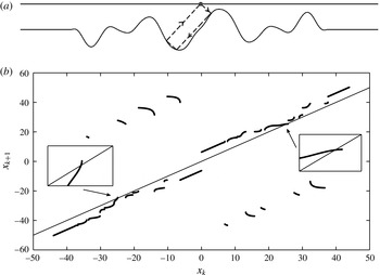
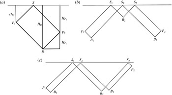
An example is shown in figure 2(a). This shows a characteristic that hits the bottom at three points before returning to the top at exactly the same point at which it started. We call this a 1-point attractor, to reflect the fact that there is only one surface point in the loop: the characteristic returns to it every time it hits the surface.
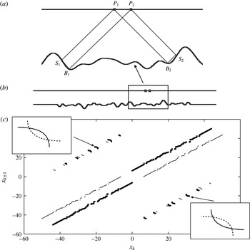
We can also have more complicated attractors. Figure 3(a) shows an example of a 2-point attractor – the characteristic starts at
 $P_{1}$
on the surface, then hits the surface at a different point
 $P_{2}$
, and on the next bounce returns to
 $P_{1}$
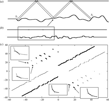
. Figure 4(a) shows a 4-point attractor, where the characteristic hits the surface at four different points, before returning to its starting point. This classification of attractors by the number of times they hit the surface closely follows that introduced in Maas & Lam (Reference Maas and Lam1995). One can see that a necessary ingredient to forming an attractor is to have at least two points where the topography is supercritical; these must then be arranged in exactly the right way.
(a) A 1-point attractor over random topography. The arrow indicates the stable direction as discussed in § 2.6. (b) The corresponding checkerboard map. The two intersections with the straight line
 $x_{k+1}=x_{k}$
correspond to the surface reflection point with characteristics moving left and right, after adopting the checkerboard map convention. The topography was generated using covariance function (3.5) with parameters
 ${\it\sigma}=1.0$
,
 ${\it\alpha}=1.2$
, over an interval of length of
 $10{\rm\pi}$
.

(a) A 2-point attractor over random topography.
 $S_{1},S_{2}$
are supercritical hitting points, while
 $B_{1},B_{2}$
are subcritical. (b) The entire bottom topography and the position of the attractor. (c) Checkerboard map that gives the 2-point attractor in (a). The solid line is the map
 $x_{k+1}=M(x_{k})$
, and the dotted line is the map
 $x_{k-1}=M^{-1}(x_{k})$
. The four intersections correspond to the two surface reflection points with right-going and left-going characteristics. The topography was generated using covariance function (3.5) with parameters
 ${\it\sigma}=0.25$
,
 ${\it\alpha}=0.5$
, over a length
 $10{\rm\pi}$
.

(a) A 4-point attractor over random topography.
 $S_{1}$
and
 $S_{2}$
are two supercritical points, while other hitting points on the bottom are subcritical. (b) The entire bottom topography, where the four dots on the surface indicate the location of the 4-point attractor. (c) Iterated checkerboard map that gives the 4-point attractor in (a). The solid line is the map
 $x_{k+2}=M^{2}(x_{k})$
, and the dotted line is the map
 $x_{k-2}=M^{-2}(x_{k})$
. The four intersections correspond to the four surface reflection points with left-going and right-going characteristics. The topography was generated using covariance function (3.5), with parameters
 ${\it\sigma}=0.25$
,
 ${\it\alpha}=0.5$
, over a length
 $10{\rm\pi}$
.

2.3. Checkerboard map
Finding attractors by following characteristics is difficult, because unless one starts at the exact location of the attractor, one will not return exactly to the starting point. Therefore, in order to determine whether a given topography contains attractors, we use a theoretical construction called the checkerboard map, introduced in Balmforth, Spiegel & Tresser (Reference Balmforth, Spiegel and Tresser1995) to study general dynamical systems and applied to internal wave attractors in Echeverri et al. (Reference Echeverri, Yokossi, Balmforth and Peacock2011). The latter analysed only 1-point attractors, so in the following sections we will show how this construction can be applied to 2- and higher-point attractors.
Roughly, the checkerboard map is a function that takes a point on the surface, and returns the next point on the surface that is hit by the corresponding characteristic. However, because there are two characteristics that emanate from each point on the surface, this function, as described, would be multi-valued. Conceptually, this is not a problem because we can distinguish the two characteristics by the direction in which they move. Mathematically and numerically, to obtain a function that is single-valued we shift each segment of this multi-valued function, where the direction of the shift depends on whether the segment describes a leftward or rightward moving characteristic. The shift is invertible, so the original multi-valued function can be recovered from the single-valued checkerboard map.
To be precise: suppose we are interested in a piece of topography described by
 $-L<x<L$
, where
 $2L$
is the horizontal extent of the surface over which we which to construct a checkerboard map, and
 $x$
is a variable describing the horizontal position on the surface. Define the shift operators
 $$\begin{eqnarray}s_{R}(x)=x+L,\quad s_{L}(x)=x-L,\end{eqnarray}$$
where the subscript ‘
 $R$
’ stands for rightward moving direction and ‘
 $L$
’ for leftward moving direction. We construct the checkerboard map
 $M(x)$
as follows. Suppose a characteristic leaves point
 $x$
heading in direction
 $i$
, and hits point
 $y$
heading in direction
 $j$
, where
 $i,j\in \{L,R\}$
. Set
 $$\begin{eqnarray}M(s_{i}(x))=s_{j}(y).\end{eqnarray}$$
For example if a characteristic leaves the surface at
 $x$
heading to the right and next hits the surface at
 $y$
while still traveling to the right, we would set
 $M(s_{R}(x))=s_{R}(y)$
. This means the segment of the original multi-valued map on which
 $(x,y)$
lies is shifted horizontally to the right by an amount
 $L$
, and vertically up by
 $L$
. If, however, a characteristic starts at
 $x^{\prime }$
, reverses its direction when it hits the bottom and next hits the surface at
 $y^{\prime }$
heading to the left, we would set
 $M(s_{R}(x^{\prime }))=s_{L}(y^{\prime })$
. Such a segment would be shifted to the right and down, each by
 $L$
. The set of points
 $\{x>0\}$
in the domain of
 $M$
represent the starting points for rightward-moving characteristics, where the actual locations on the surface are found as
 $x-L$
, while
 $\{x<0\}$
represent the starting points for leftward-moving characteristics, whose actual surface locations are
 $x+L$
. In this way, we obtain a single-valued function
 $M(x)$
, such that the iterations
 $M\circ M\circ \cdots \circ M(x)$
record the successive hitting points on the surface combined with their direction of motion.
We have built a code that computes the checkerboard map numerically over arbitrary topography. This is a challenge, because one has to carefully resolve the curvature of the topography to find all the hitting points of the characteristics. The numerical method is described in appendix A.
This method was used to compute the checkerboard map for each sample of random topography. Two examples and the corresponding topographies are shown in figures 2, 3 (solid lines). These maps are made of piecewise continuous segments, broken up by many discontinuities. Each discontinuity (except at
 $x=0$
) comes from a critical point of the topography, where the slope is exactly 1. Specifically, each concave critical point gives rise to three discontinuities in the checkerboard map, one for each of the three characteristics that emanate from the point unobstructed. Characteristics that are slightly perturbed from one of these three will be reflected in one of the other two directions, depending on the sign of the perturbation.
2.4. Detecting attractors
We can use the checkerboard map to find attractors and their topological characterizations.
A 1-point attractor occurs when a point on the surface is mapped to the same point under the checkerboard map. This corresponds to the solution of
 $M(x)=x$
: it is a fixed point of the checkerboard map. To find these, we must check whether
 $M(x)$
intersects the straight line
 $y=x$
. In figure 2(b), we find two such intersections (highlighted in boxes), one for each direction along which the attractor can be followed.
A 2-point attractor occurs when a point on the surface returns to itself after two iterations of the checkerboard map. This corresponds to the solution of
 $M^{2}(x)=x$
, where
 $M^{2}=M\circ M$
. An example of the map
 $M^{2}$
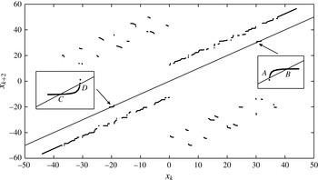
is shown in figure 5. There are now four intersections corresponding to the single attractor: one for each point on the surface, and each of these has two intersections, for the leftward and rightward going characteristics.
Finding 2-point attractors by computing
 $M^{2}$
allows for a nice theoretical analysis but has a few shortcomings in practice. We only know a discretized version of the checkerboard map, so we compute its value at an arbitrary point
 $x$
by linear interpolation. This induces a small error, and since the map is quite sensitive to the location of the discontinuities, this can create or destroy some potential intersection points.
An alternative method is to look for solutions to
 $M(x)=M^{-1}(x)$
. This method is numerically more robust, because no additional approximation is needed after finding the checkerboard map:
 $M^{-1}$
can be obtained easily by reflection about the line
 $y=x$
. Figure 3(b) shows
 $M,M^{-1}$
, and highlights the four intersection points, in boxes.
A similar method can be used to find attractors involving more reflection points on the surface. For the 4-point attractor, we do not compute fixed points of the map
 $M^{4}(x)=x$
, but rather seek the intersection points of
 $M^{2}(x)$
and
 $M^{-2}(x)$
; only one interpolation process is needed. Figure 4(c) shows these two maps along with the 8 intersection points corresponding to the 4-point attractor.
2.5. There are no. 1- and 3-point attractors
Interestingly, we cannot have 1-point or 3-point attractors with small amplitude topography. An explanation for this is as follows. Let
 ${\it\Delta}=\max |h(x)|$
be the largest height of the topography. Let
 $P_{1},P_{2}$
be two supercritical points and let
 $B$
be the subcritical point on the closed orbit of an attractor (see figure 6). The distance from
 $P_{1}$
,
 $P_{2}$
and
 $B$
to the surface are given by
 $H_{P_{1}}={\rm\pi}+{\it\alpha}{\it\Delta}$
,
 $H_{P_{2}}={\rm\pi}+{\it\beta}{\it\Delta}$
and
 $H_{B}={\rm\pi}+{\it\gamma}{\it\Delta}$
where
 ${\it\alpha},{\it\beta}$
and
 ${\it\gamma}$
are parameters that vary between
 $-1$
and
 $1$
. From figure 6, these three distances satisfy
 $H_{P_{1}}+H_{P_{2}}=H_{B}$
. By simple algebra, we have
 $3{\it\Delta}>({\it\gamma}-{\it\alpha}-{\it\beta}){\it\Delta}={\rm\pi}$
, which requires
 ${\it\Delta}>{\rm\pi}/3$
. If we model the topography by a Gaussian process and assume the largest deviation
 ${\it\Delta}$
is approximately three times the standard deviation
 ${\it\sigma}$
, then we need
 ${\it\sigma}>{\rm\pi}/9\approx 0.35$
.
The iterated checkerboard map
 $x_{k+2}=\mathscr{M}^{2}(x_{k})$
near the fixed points/surface reflection points of the random topography in figure 3.

A similar argument applied to a 3-point attractor (examples are sketched in figure 6) suggests we need
 ${\it\Delta}>{\rm\pi}/5$
or
 ${\it\sigma}>{\rm\pi}/15\approx 0.21$
to have 3-point attractor.
Hence small-amplitude topography, whose non-dimensional standard deviation is much less than
 ${\rm\pi}$
, is very unlikely to contain a 1-point or 3-point attractor. We had to use topography with a large standard deviation (
 ${\it\sigma}=1$
) to see the 1-point attractor in figure 2, and topography in the ocean with this large an amplitude is probably not well modelled by a Gaussian process.
Notice that there are no height constraints on the topography for an even-numbered attractor. Some insight into this comes from considering the amount each characteristic is displaced every time it returns to the surface. This random quantity is equal to
 $\pm 2{\rm\pi}+{\it\xi}$
or
 ${\it\xi}$
depending on whether it hits zero or one supercritical points on the bottom, respectively, where
 ${\it\xi}$
is a random variable related to the height deviations of the hitting points on the bottom. For example, if the characteristic hits only one (necessarily subcritical) point on the bottom, then
 $|{\it\xi}|$
is twice the height of that point. If the characteristic hits one subcritical and one supercritical point, then
 $|{\it\xi}|$
is twice the absolute difference in height between those points.
An even-numbered attractor can be formed by a characteristic that hits two supercritical points at either end, with an even number of purely subcritical bounces in between. The factors of
 $\pm 2{\rm\pi}$
cancel in the sum of the displacements, so an attractor occurs when
 ${\it\xi}_{1}+\cdots +{\it\xi}_{2k}=0$
. This is possible with reasonable probability even if the random variables are small.
An odd-numbered attractor generally requires an odd number of purely subcritical bounces (with the exception of the 1-point attractor, which requires a separate argument), so we need
 ${\it\xi}_{1}+\cdots +{\it\xi}_{2k+1}=\pm 2{\rm\pi}$
. If the height differences
 ${\it\xi}_{i}$
are typically small, this event is very unlikely.
2.6. Stability of attractors
We remark briefly on the reason for calling these closed orbits ‘attractors’. It is well-known that a 1-point attractor acts as a dynamical attractor for nearby characteristics, whose stability depends on the direction of the characteristics: those that start near the point on the surface and move to the right will be either attracted to it or repelled from it, while those that start nearby and move to the left will do the opposite (Echeverri et al. Reference Echeverri, Yokossi, Balmforth and Peacock2011). We are not aware of an analysis for higher-point attractors, so provide an explicit calculation here of the 2-point attractors. We show these are stable for characteristics moving in one direction around the loop, and unstable for characteristics moving in the other direction.
(a) Sketch of a 1-point attractor illustrating the argument in § 2.5.
 $P_{1}$
and
 $P_{2}$
are two supercritical points and
 $B$
is the subcritical point on the closed orbit.
 $H_{P_{1}}$
,
 $H_{P_{2}}$
and
 $H_{B}$
are their distance to the surface at
 $h={\rm\pi}$
.
 $S$
is the corresponding surface point. (b,c) Two examples of a 3-point attractor,
 $S_{i}$
are surface points,
 $P_{i}$
are supercritical bottom points and
 $B_{i}$
are subcritical bottom points.

Recall that a fixed point
 $x_{0}$
of a map
 $\mathscr{F}:\mathbb{R}\rightarrow \mathbb{R}$
is stable if
 $|\mathscr{F}^{\prime }(x_{0})|<1$
. For a 2-point attractor, we must compute the derivative of the map
 $\mathscr{F}(x)=M^{2}(x)$
.
Suppose a 2-point attractor involves points
 $P_{1}$
,
 $P_{2}$
on the surface, as in figure 3. The checkerboard map satisfies
 $$\begin{eqnarray}M(P_{1}+\,L)=P_{2}-L,\!\quad M(P_{1}-L)=P_{2}+L,\!\quad M(P_{2}+L)=P_{1}-L,\!\quad M(P_{2}-L)=P_{1}+\,L.\end{eqnarray}$$
This gives rise to four fixed points of
 $M^{2}$
:
 $P_{1}\pm L$
,
 $P_{2}\pm L$
. The map
 $M^{2}$
is shown in figure 5, where the fixed points are labelled
 $A$
(
 $P_{1}+L$
),
 $B$
(
 $P_{2}+L$
),
 $C$
(
 $P_{1}-L$
) and
 $D$
 $(P_{2}-L)$
. Consider a characteristic that leaves
 $P_{1}$
heading to the left (this is point
 $B$
in figure 5), hits points
 $S_{1},B_{1}$
on the bottom before hitting
 $P_{2}$
heading to the right (point
 $C$
in figure 5) and in the other direction hits
 $S_{2},B_{2}$
. Here the points
 $S_{i}$
are supercritical and
 $B_{i}$
are subcritical, as in figure 3. (In general a 2-point attractor could be more complicated, but we consider only the simplest case.) The points are related as (using labels to denote the horizontal positions)
 $$\begin{eqnarray}h(S_{1})-S_{1}={\rm\pi}-P_{1},\quad h(S_{1})+S_{1}=h(B_{1})+B_{1},\quad h(B_{1})-B_{1}={\rm\pi}-P_{2}.\end{eqnarray}$$
Differentiating these equations implicitly, we find
 $M^{\prime }(C)\!=\text{d}P_{2}/\text{d}P_{1}=((1-|h^{\prime }(S_{1})|)/(1+|h^{\prime }(S_{1})|))(1-h^{\prime }(B_{1}))/(1+h^{\prime }(B_{1}))$
. (We include an absolute value to account for the general case, where
 $S_{1}$
could be on the right, so some of the signs of (2.8) would be changed accordingly.) In a similar manner, we can calculate
 $M^{\prime }(B)=((1-|h^{\prime }(S_{2})|)/(1+|h^{\prime }(S_{2})|))(1+h^{\prime }(B_{2}))/(1-h^{\prime }(B_{2}))$
. Putting this together and noting that
 $M(B)=C$
,
 $M(C)=B$
gives the slope of
 $M^{2}$
at
 $B$
,
 $C$
as
 $$\begin{eqnarray}d=\frac{1-|h^{\prime }(S_{1})|}{1+|h^{\prime }(S_{1})|}\frac{1-h^{\prime }(B_{1})}{1+h^{\prime }(B_{1})}\frac{1-|h^{\prime }(S_{2})|}{1+|h^{\prime }(S_{2})|}\frac{1+h^{\prime }(B_{2})}{1-h^{\prime }(B_{2})}.\end{eqnarray}$$
Similarly, one can calculate the slope at
 $A$
,
 $D$
to be
 $1/d$
. Therefore if
 $d>1$
, then a characteristic that starts at
 $P_{1}$
and moves to the left around the loop is stable, but one that moves to the right is unstable. If
 $d<1$
the stabilities are reversed.
We briefly note (omitting the details) that this can also be derived through a geometrical argument that considers how the separation between nearby characteristics changes each time they reflect off a straight line with a given slope. If they hit a subcritical point
 $B$
from left to right (positive direction), the separation changes by a factor of
 $(1-h^{\prime }(B))/(1+h^{\prime }(B))$
. If they hit a supercritical point
 $S$
from up to down, the change is
 $(1-|h^{\prime }(S)|)/(1+|h^{\prime }(S)|)$
. If the directions of either are reversed, the factor is inverted. One can multiply the factors at all hitting points together to obtain the derivative of the checkerboard map. Since the factors are inverted upon direction reversal, the stability will be reversed.
3. Rate of attractors
What is the probability of finding an attractor in a given stretch of topography? Since attractors may cause enhanced scattering and mixing, this question is central to understanding whether they play a role in energy transfer in the ocean over rough topography. The answer will depend on the statistics of the topography, such as the distribution of heights, slopes and higher-order shape information. In this section, we investigate how the probability of finding an attractor depends on these parameters.
We model the topography as a stationary, zero-mean, Gaussian random process. Such a process is characterized by its covariance function
 $C(x)$
, defined by
 $$\begin{eqnarray}C(x)=\mathbb{E}h(y)h(x+y),\end{eqnarray}$$
where
 $\mathbb{E}$
is the probabilistic expectation (note that
 $\mathbb{E}h(x)=0$
). The covariance function is related to the spectral density
 ${\hat{C}}(k)$
by the Fourier transform:
 $$\begin{eqnarray}{\hat{C}}(k)=\int _{-\infty }^{\infty }C(x)\text{e}^{-\text{i}kx}\,\text{d}x,\quad C(x)=\frac{1}{2{\rm\pi}}\int _{-\infty }^{\infty }{\hat{C}}(k)\text{e}^{\text{i}kx}\,\text{d}k.\end{eqnarray}$$
We generate topography
 $h(x)$
on the interval
 $x\in [-L_{x}/2,L_{x}/2]$
with covariance function a periodic approximation to
 $C(x)$
, by first generating a complex-valued stationary Gaussian random process
 $H(x)$
with covariance function
 $C_{H}(x)=2C(x)=\mathbb{E}H(y)\overline{H(x+y)}$
. This is easily done by computing its Fourier coefficients (Yaglom Reference Yaglom1962)
 $$\begin{eqnarray}{\hat{H}}(k)=\sqrt{\frac{L_{x}{\hat{C}}_{H}(k)}{2}}(A_{k}+\text{i}B_{k}),\quad \text{so that }H(x)=\frac{{\rm\Delta}k}{2{\rm\pi}}\mathop{\sum }_{n=-N/2+1}^{N/2}{\hat{H}}(n)\text{e}^{\text{i}n{\rm\Delta}kx}.\end{eqnarray}$$
Here
 $A_{k}$
and
 $B_{k}$
are independent Gaussian random variables with mean
 $0$
and variance
 $1$
,
 $N$
is the number of points used to represent the topography and
 ${\rm\Delta}k=2{\rm\pi}/L_{x}$
. The numerical values of the parameters we use are listed in appendix A.
The real-valued topography is found by taking the real or imaginary part: if
 $H=h_{1}+\text{i}h_{2}$
is a complex Gaussian random process with covariance function
 $2C(x)$
, then
 $h_{1}$
and
 $h_{2}$
are independent, real-valued Gaussian random processes with covariance function
 $C(x)$
(Hida & Hitsuda Reference Hida and Hitsuda1993).
From the spectral representation of
 $h$
, we can easily find the spectral density and covariance function of its slope
 $h^{\prime }$
via (Yaglom Reference Yaglom1962)
 $$\begin{eqnarray}{\hat{C}}_{h^{\prime }}(k)=k^{2}{\hat{C}}(k),\quad C_{h^{\prime }}(x)=-C^{\prime \prime }(x).\end{eqnarray}$$
For each given covariance function, we compute the rate of attractors, defined to be the average number of attractors in an interval of length
 $2{\rm\pi}$
. We do this by generating
 $N_{s}$
samples of the topography on an interval of length
 $L_{x}=10{\rm\pi}$
, and then counting the number of attractors that lie in the middle interval of length
 $8{\rm\pi}$
. By discarding the intervals at the end, we remove boundary effects due to characteristics hitting the flat topography outside the
 $10{\rm\pi}$
interval. The rate of attractors is then the total number of attractors found in all samples, divided by
 $4N_{s}$
(
 $=(8{\rm\pi}/2{\rm\pi})N_{s}$
).
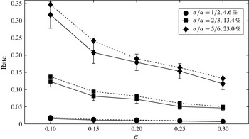
Rate of 2-point attractors from direct numerical Monte Carlo simulations (solid lines), with 95 % confidence levels given by
 $(\text{no. of attractors}\pm 1.96\cdot \sqrt{\text{no. of attractors}})/(4N_{s})$
. Dotted lines indicate the result from Rice’s formula (4.2). See appendix B for numerical values of the data.

The most common attractor in our numerical simulations is the 2-point attractor. Figure 7 shows the result of simulations using the covariance function that is Gaussian-shaped, in both real and spectral space:
 $$\begin{eqnarray}C_{g}(x)={\it\sigma}^{2}\exp \left(-\frac{x^{2}}{2{\it\alpha}^{2}}\right)\quad \Rightarrow \quad {\hat{C}}_{g}(k)=\sqrt{2{\rm\pi}}{\it\sigma}^{2}{\it\alpha}\exp \left(-\frac{k^{2}{\it\alpha}^{2}}{2}\right).\end{eqnarray}$$
This has two parameters,
 ${\it\sigma},{\it\alpha}$
controlling the height and horizontal scale of the topography, respectively. The height and slope at a single location are zero-mean Gaussian random variables with variances (leaving the subscript off, as we will use this relationship for other covariance functions)
 $$\begin{eqnarray}\mathbb{E}h^{2}=C(0)={\it\sigma}^{2},\quad \mathbb{E}h^{\prime 2}=-C^{\prime \prime }(0)={\it\sigma}^{2}/{\it\alpha}^{2}.\end{eqnarray}$$
The ratio
 ${\it\sigma}/{\it\alpha}$
controls the fraction of supercritical topography.
In our simulations we consider what happens when we decrease
 ${\it\sigma}$
,
 ${\it\alpha}$
with
 ${\it\sigma}/{\it\alpha}$
fixed. Figure 7 shows three experiments with supercritical probabilities of 4.6 %, 13.4 %, 23.0 %, where all values of
 ${\it\alpha}$
under consideration are small enough that the topography at subsequent subcritical bounces of a characteristic is effectively uncorrelated with itself (numerical values of the data are shown in appendix B). For fixed
 ${\it\sigma}$
, the rate of 2-point attractors strictly increases with the supercritical fraction. This should be expected, because there are more supercritical points that can align in the right way to give an attractor. Interestingly, for fixed
 ${\it\sigma}/{\it\alpha}$
, the rate of 2-point attractors increases as
 ${\it\sigma}$
decreases, or equivalently as
 ${\it\alpha}$
decreases. Since
 ${\it\alpha}$
controls the correlation length of the topography, as it decreases the topography becomes rougher and rougher while maintaining the same supercritical fraction. It is not obvious why the number of attractors should increase, though we attempt a rough explanation in the next section.
We investigate whether this observation holds for other shapes of the topography by considering two different covariance functions. One is exponential in spectral space, given by
 $$\begin{eqnarray}{\hat{C}}_{e}(k)=\sqrt{2}{\rm\pi}{\it\sigma}^{2}{\it\alpha}\exp \left\{-\sqrt{2}{\it\alpha}|k|\right\},\quad C_{e}(x)=\frac{{\it\sigma}^{2}}{1+x^{2}/(2{\it\alpha}^{2})}.\end{eqnarray}$$
The parameters
 ${\it\sigma},{\it\alpha}$
have the same relation (3.6) to the height and slope. A second is the spectrum for Bell’s topography, used to model the topography in the abyssal hills regions of the North Pacific (Bell Reference Bell1975b
). This spectrum is formulated for two-dimensional topography, so to apply it to our one-dimensional model we consider the marginal spectrum along a transect, assuming the topography is isotropic. In spectral space, the covariance function is (see appendix D)
 $$\begin{eqnarray}{\hat{C}}_{B}(k)=A\frac{{\it\kappa}_{1}}{\sqrt{{\it\kappa}_{1}^{2}+{\it\kappa}_{2}^{2}}}\frac{\sqrt{{\it\kappa}_{2}^{2}-k^{2}}}{k^{2}+{\it\kappa}_{1}^{2}},\quad |k|<{\it\kappa}_{2}.\end{eqnarray}$$
This contains three parameters:
 $A,{\it\kappa}_{1},{\it\kappa}_{2}$
. The parameter
 $A$
controls the height of the topography,
 ${\it\kappa}_{1}=2{\rm\pi}/40~\text{km}$
controls the correlation length of the topography and
 ${\it\kappa}_{2}=2{\rm\pi}/400~\text{m}$
is a cutoff scale so that the topography has finite derivative. Bell (Reference Bell1975b
) suggests
 $k_{2}=100k_{1}$
, but we choose
 $k_{2}=20k_{1}$
so the spectrum is easier to resolve numerically. If we identify parameters
 ${\it\sigma},{\it\alpha}$
to have the same meaning as in (3.6), then these are related to Bell’s parameters as
 $$\begin{eqnarray}k_{1}\approx \frac{0.3242}{{\it\alpha}},\quad A\approx 1.0526\cdot 2{\it\sigma}^{2}\end{eqnarray}$$
but their values can be exactly calculated as shown in appendix D. The main qualitative difference from the Gaussian and exponential covariance functions is that this has a power-law decay in spectral space, hence a heavier tail, and so larger higher-order moments.
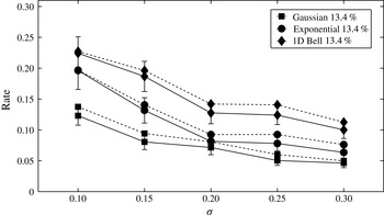
Rate of attractors for different covariance functions with
 ${\it\sigma}/{\it\alpha}=2/3$
. Solid lines are predicted by direct numerical simulations. Dotted lines are from Rice’s formula (4.2).

Figure 8 compares the rate of 2-point attractors for all three covariance functions, with the fraction of supercritical topography set at 13.4 %. We see the same trend, with the rate increasing monotonically as
 ${\it\sigma}$
decreases. For all values of
 ${\it\sigma}$
, the Gaussian covariance function has the lowest rate, while Bell’s spectrum has the highest, at approximately double the Gaussian rate. The ordering is consistent with the decay of the covariance functions in spectral space, with the Gaussian covariance function decaying most rapidly and Bell’s spectrum decaying the least. For fixed
 ${\it\sigma}$
, all three ensembles of topographies have the same height and slope densities at a point, so this suggests that higher-order derivatives are also important in determining the rate of attractors.
We have also looked for 4-point attractors, but these are much less likely. For example, for topography with Gaussian covariance function
 $C_{g}$
and
 ${\it\sigma}=0.25$
, at 4.6 % supercritical fraction we found 39 4-point attractors in a sample of 6000 (compared to 198 2-point attractors, see table 1 in appendix B), at 13.4 % supercritical fraction we found 37 4-point attractors in a sample of 800 (compared to 161 2-point attractors) and at 23.0 % supercritical fraction we found 25 4-point attractors in a sample of 300 (compared to 184 2-point attractors). We verified each of these 4-point attractors by eye as the method found several incorrect attractors that were created by the numerical interpolation. Since detecting 4-point attractors is numerically less robust, and since they are probably also less robust in the ocean because they exist over longer scales, we do not analyse the rate of 4-point attractors here but merely point out that they can and do exist.
We never found a 1-point or 3-point attractor in the type of simulations described above, consistent with our argument in § 2.5.
4. Rice’s formula for the rate of attractors
How can we understand and interpret the numerical results in § 3? Predicting the rate of attractors theoretically is a challenge, because this is a highly nonlinear problem that is hard to reduce to a small number of parameters characterizing the local shape of the topography, such as the variance of its derivatives at a point. One can imagine approximating the topography locally, for example using its maximum likelihood shape near hitting points on the bottom, and using this to calculate when an attractor occurs. However, any theory must ultimately be based on a formula for the rate at which a stochastic process behaves in a certain way, so in this section we investigate whether it is possible to identify such a formula.
We focus on 2-point attractors. If we define a stochastic process
 $S(t)$
by
 $$\begin{eqnarray}S(t)=M^{2}(t)-t,\end{eqnarray}$$
then a 2-point attractor occurs each time
 $S(t)=0$
. Therefore, the problem of calculating the rate of attractors is equivalent to that of calculating the rate of zero crossings of
 $S(t)$
.
When
 $S(t)$
is a stationary, continuously differentiable stochastic process (this formula can be generalized; see Adler & Taylor (Reference Adler and Taylor2007)) then there is a well-known result, Rice’s formula, that gives the rate of crossing a level
 $S(t)=u$
:
 $$\begin{eqnarray}\text{rate}=\mathbb{E}\frac{\text{no. of crossings}}{2{\rm\pi}\text{-interval}}=2{\rm\pi}\int _{-\infty }^{\infty }|v|p(u,v)\,\text{d}v,\end{eqnarray}$$
where
 $p(u,v)$
is the joint density of
 $S(t),S^{\prime }(t)$
at a point (Rice Reference Rice1945; Adler & Taylor Reference Adler and Taylor2007). The process
 $S(t)$
defined by (4.1) can be reasonably expected to be stationary since it is constructed from a stationary process (the topography), but it is certainly not continuously differentiable, nor even continuous. However, it is piecewise continuously differentiable, and if the pieces are sufficiently ‘independent’, one might expect the formula to still be valid. Indeed, we argue in appendix E that if the jumps occur as a Poisson process, and are independent of
 $S$
and
 $S^{\prime }$
, then Rice’s formula (4.2) should still hold.
We investigate whether Rice’s formula can predict the number of attractors by numerically computing the joint density
 $p(u,v)$
of
 $S,S^{\prime }$
and the integral (4.2) with
 $u=0$
(see appendix C). The rates predicted by Rice’s formula for the Gaussian covariance function (3.5) are shown in figure 7, and for the three covariance functions (3.5), (3.7), (3.8) in figure 8 (see appendix B for numerical data). These are close to the rates from the Monte Carlo simulations – Rice’s formula consistently overpredicts the rate, by 5–15 %, with a maximum discrepancy of 22 % occurring for the topography with the smallest supercritical fraction. In particular, Rice’s formula shows the same trend when
 ${\it\sigma}/{\it\alpha}$
is held constant, with the rate increasing as
 ${\it\sigma}$
decreases.
The discrepancy between Rice’s formula and the simulated rates is thought to arise from two sources. One is numerical – the result of interpolating the checkerboard map and approximating its derivative. The other is because the discontinuities in
 $S(t)$
are not independent of the values of
 $S$
,
 $S^{\prime }$
– the jumps occur exactly when the topography has slope
 $\pm 1$
, and this in turn is related to the behaviour of the checkerboard map, as near the discontinuous point
 $S^{\prime }$
is either very small (
 ${\approx}0$
) or very large (
 ${\approx}\infty$
). The statistical error that arises from the finite sample size is expected to be fairly low.
Because of this close agreement, we can use Rice’s formula to try to understand the qualitative behaviour of the rates as
 ${\it\sigma}$
decreases with
 ${\it\sigma}/{\it\alpha}$
held constant. First, we consider a simpler process: a zero-mean, stationary Gaussian stochastic process
 $h(t)$
(such as the topography), and ask how the rate of zero-crossing changes as the process is squished both horizontally and vertically in such a way that its slope distribution stays the same. Mathematically, this can be achieved by the transformation
 $h(t)\rightarrow h^{{\it\sigma}}(t)={\it\sigma}h(t/{\it\sigma})$
, with
 ${\it\sigma}<1$
. The number of zero crossings only depends on the horizontal stretching factor, so it will increase by a factor of
 ${\it\sigma}^{-1}$
. In Rice’s formula, this factor emerges from the way the marginal densities of height and slope transform under the scaling. The marginal density of the slope
 $h^{\prime }$
at a point (call this
 $p_{h^{\prime }}^{{\it\sigma}}(v)$
) is constant under the scaling transformation, so
 $p_{h^{\prime }}^{{\it\sigma}}(v)=p_{h^{\prime }}^{1}(v)$
. The marginal density of the value of the process transforms as
 $p_{h}^{{\it\sigma}}(u)={\it\sigma}^{-1}p_{h}^{1}(u/{\it\sigma})$
, so it has a higher density at 0. The values of
 $h^{{\it\sigma}}$
,
 $\text{d}h^{{\it\sigma}}/\text{d}x$
at a point are independent random variables (since the process is Gaussian), so the joint density factors as
 $p^{{\it\sigma}}(u,v)=p_{h}^{{\it\sigma}}(u)p_{h^{\prime }}^{{\it\sigma}}(v)$
. Substituting for the marginals and using Rice’s formula (4.2) gives the scaling factor
 ${\it\sigma}^{-1}$
.
Next consider how the function
 $S(t)$
transforms while the topography is scaled with
 ${\it\sigma}$
, as above. This process does not transform in such a simple way as
 $h$
, yet we will argue that the marginal densities scale in qualitatively the same way: the marginal density of
 $S$
near 0 increases, while the marginal density of
 $S^{\prime }$
remains approximately constant. If the joint density approximately factors into a product of marginals, the rate will increase. Physically this means the iterated checkerboard map has smaller relative displacements but the slope is constant, in probability. Therefore it crosses zero more frequently, since it is easier for a sum of small random variables to equal zero than a sum of occasionally larger ones.
To argue this we must find explicit expressions for
 $S$
,
 $S^{\prime }$
. Let us define the ‘shift’ map
 ${\it\theta}(t)=M(t)-t$
to be the amount that a characteristic is shifted from its starting position after each return to the surface (we ignore the operators
 $s_{L}$
,
 $s_{R}$
from (2.5) in this section because they do not affect the argument). It is related to the process of interest by
 $$\begin{eqnarray}S(t)={\it\theta}({\it\theta}(t)+t)+{\it\theta}(t),\quad S^{\prime }(t)={\it\theta}^{\prime }({\it\theta}(t)+t)({\it\theta}^{\prime }(t)+1)+{\it\theta}^{\prime }(t).\end{eqnarray}$$
In figure 3(a), the characteristic starting from the point
 $P_{1}$
on the surface leaves to the left, hits the bottom at supercritical point
 $S_{1}$
, then hits subcritical point
 $B_{1}$
and returns to the surface point
 $P_{2}$
. We need two such events to happen to create an attractor, so must analyse how
 ${\it\theta}(t)$
behaves in this situation.
The points
 $P_{1},S_{1},B_{1}$
and
 $P_{2}$
are related by (2.8), from which we compute the shift map to be
 $$\begin{eqnarray}{\it\theta}(P_{1})=P_{2}-P_{1}=h(S_{1})-h(B_{1})-(S_{1}-B_{1}).\end{eqnarray}$$
As the topography is scaled by letting
 ${\it\sigma}$
decrease, we expect the random variables
 $h(S_{1})-h(B_{1})$
and
 $S_{1}-B_{1}$
to become smaller, on average. Therefore, the marginal density of
 ${\it\theta}$
should become more peaked near 0. From (4.3) we have that
 $S(t)$
is the sum of two copies of this random variable (evaluated at locations
 $t$
and
 ${\it\theta}(t)+t$
), so the marginal density of
 $S$
should also have a higher density near zero. Suppose the density increases by some factor
 ${\it\beta}^{-1}>1$
, so we can write
 $p_{S}^{{\it\sigma}}(0)\approx {\it\beta}^{-1}p_{S}^{1}(0)$
.
Next consider how
 $S^{\prime }$
and
 ${\it\theta}^{\prime }$
behave with
 ${\it\sigma}$
. From (2.8) we compute
 $$\begin{eqnarray}{\it\theta}^{\prime }(P_{1})=\frac{\text{d}P_{2}}{\text{d}P_{1}}-1=\frac{1+h^{\prime }(S_{1})}{1-h^{\prime }(S_{1})}\frac{1-h^{\prime }(B_{1})}{1+h^{\prime }(B_{1})}-1.\end{eqnarray}$$
This only depends on the pointwise derivatives of the topography, whose probability densities do not change with
 ${\it\sigma}$
. If
 $h(S_{1})$
and
 $h(B_{1})$
maintain roughly the same correlation after scaling by
 ${\it\sigma}$
, then the density of
 ${\it\theta}^{\prime }(P_{1})$
will remain approximately invariant with
 ${\it\sigma}$
, and by (4.3) so will that of
 $S^{\prime }$
.
If we approximate the joint density of
 $S,S^{\prime }$
as a product of the marginal densities, then we find the scaled density at
 $S=0$
behaves roughly as
 $$\begin{eqnarray}p^{{\it\sigma}}(0,v)\approx p_{S}^{{\it\sigma}}(0)p_{S^{\prime }}^{{\it\sigma}}(v)\approx {\it\beta}^{-1}p_{S}^{1}(0)p_{S^{\prime }}^{1}(v),\end{eqnarray}$$
By (4.2) this implies the rate of zero crossings is scaled by
 ${\it\beta}^{-1}$
: it increases as
 ${\it\sigma}$
decreases.
5. Discussion
Let us estimate how prevalent attractors might be over certain rough, small-scale features in the ocean. As an example, we take Bell’s spectrum for the abyssal hill region of the ocean basin in the Eastern central North Pacific. While this is not expected to be quantitatively accurate for the entire ocean basin, it gives us some representative numbers that are within an order of magnitude of many realistic spectra. To apply this, we need to estimate the fraction of topography that is supercritical and its non-dimensional standard deviation. Using the same parameters as in Bell (Reference Bell1975b
), the variance of the two-dimensional topography slope is
 $\mathbb{E}|\boldsymbol{{\rm\nabla}}\tilde{h}|^{2}\approx (125\,m)^{2}{\it\kappa}_{1}{\it\kappa}_{2}\approx 0.2^{2}$
, where
 ${\it\kappa}_{1}=2{\rm\pi}/40~\text{km}$
and the effective cutoff wavenumber
 ${\it\kappa}_{2}=2{\rm\pi}/400~\text{m}$
. Assuming the topography is isotropic, so each of the two parts of the derivative have the same expected value, the one-dimensional model topography has
 $$\begin{eqnarray}\mathbb{E}|\tilde{h}^{\prime }|^{2}\approx (125\,m)^{2}{\it\kappa}_{1}{\it\kappa}_{2}/2\approx 0.14^{2}.\end{eqnarray}$$
A typical value of the slope of the characteristics before non-dimensionalization is
 ${\it\mu}=0.17$
, based on
 ${\it\omega}/f=2$
, the value for the semi-diurnal tide, and
 $N/f\approx 10$
. If we assume the bottom is modelled as a zero-mean stationary Gaussian process with standard deviation 0.14, then approximately
 $22.5\,\%$
of the ocean bathymetry is supercritical. Using
 ${\it\sigma}=125$
m and a typical height of
 $H=4$
km gives a non-dimensional variance of
 ${\it\sigma}^{\prime }=0.1$
.
We simulated the rate of attractors using Bell’s spectrum with the standard deviation and supercritical fraction above (
 ${\it\sigma}=0.1$
,
 ${\it\sigma}/{\it\alpha}=22.5\,\%$
). The simulated non-dimensional rate of 2-point attractors was
 $0.5\text{ attractors}/2{\rm\pi}$
, which gives a dimensional rate of
 $0.01\text{ attractors}~\text{km}^{-1}$
. This estimate is conservative, since our simulations used a lower cutoff wavenumber than Bell’s actual topography and our results suggest that broadening the spectrum (at fixed height, slope) will also increase the rate.
Therefore, if a mode-1 internal tide travels 1000 km, this model predicts it would encounter approximately 10 attractors, on average. This number is large enough to suggest that attractors over small-scale topography may be a real phenomenon. However, whether this number is quantitatively significant depends on how much dissipation attractors induce. A relevant calculation would therefore be to estimate the average dissipation of the internal tide due to a single attractor.
To do this, one needs to regularize the problem by adding a dissipative term such as viscosity. This thickens the attractor, creating a flow with sharp gradients in the vicinity. In these regions, there is enhanced vorticity and hence dissipation, since the dissipation is the vorticity squared time the viscosity integrated over the area near an attractor (Ogilvie Reference Ogilvie2005). It may be possible to solve for the leading-order structure of the flow, for example as Rieutord et al. (Reference Rieutord, Georgeot and Valdettaro2001), Ogilvie (Reference Ogilvie2005) have done for attractors in closed geometries, and from this obtain an estimate of the dissipation. Interestingly, Ogilvie (Reference Ogilvie2005) has found that the total dissipation approaches an
 $O(1)$
constant as the size of the dissipative term is decreased to zero, where the constant appears to be independent of the exact form of the dissipation.
The calculations of Ogilvie (Reference Ogilvie2005) found that the width of the region of sharp gradients near the attractor depends not only on the size of the regularization term, but also on the focussing power of the attractor: characteristics are focussed at some rate
 ${\it\alpha}$
(in his notation) by the hyperbolic terms in the equation, but they are spread out by the viscous terms. The width of the sharp region behaved as
 $\log {\it\alpha}$
and the total dissipation as
 $1/\log {\it\alpha}$
. This suggests that the total dissipation could depend not only on the average number of attractors, but also on geometrical properties, such as the average focussing rate, the size of the basins of attraction and so on.
If this calculation shows that attractors lead to an amount of dissipation that is locally larger than the background amount due to scattering, then they could even dominate the dissipation over rough topography. Mathur et al. (Reference Mathur, Carter and Peacock2014) showed that the tidal scattering along a one-dimensional transect of small-amplitude ocean bathymetry appears to be controlled by the largest feature along the path, so if an attractor has the same impact on energy dissipation as an unusually large feature on the bottom on the ocean, then these could play a key role in controlling the energy dissipation over small-scale, rough topography. Of course, whether or not this is actually the case has yet to be determined.
The above discussion applies only to one-dimensional random topography, yet since it appears that attractors can occur in this setting, an interesting and important problem would be to consider attractors over two-dimensional topography. Some progress has been made in this direction by following wave packets that bounce around inside a three-dimensional domain (Rieutord et al. Reference Rieutord, Georgeot and Valdettaro2001; Manders & Maas Reference Manders and Maas2004; Rabitti & Maas Reference Rabitti and Maas2013, Reference Rabitti and Maas2014), and numerical simulations of the barotropic tide with dissipation have found significantly reduced energy flux through a channel when it contains an attractor for these three-dimensional ray-tracing dynamics (Drijfhout & Maas Reference Drijfhout and Maas2007). These are promising studies yet it is not completely understood why they work, since rays do not necessarily give the same information as the characteristics of the equations themselves. In three dimensions, each point on the bottom is associated with a characteristic ‘cone’ along which information propagates, rather than two characteristic lines, and it is not clear whether selecting particular lines in this cone is sufficient to capture the relevant energy focussing properties.
One must also keep in mind that this model should only be applied to topography above a certain horizontal scale – the linear fluid equations are valid when the tidal excursion
 $U/{\it\omega}$
(where
 $U$
is the horizontal tidal velocity) is much smaller than the typical scale of the topography, so we cannot include the smallest scales of the topography in a realistic model. It is not clear exactly how the topography should be smoothed for the purpose of modelling attractors.
We have made a number of other simplifying assumptions to obtain a tractable, though idealized, model. One of these is constant
 $N$
,
 $f$
, as discussed in the introduction. Even if we let these be locally constant, one might wonder what happens as they vary. The only effect is to change the slope
 ${\it\mu}$
of the characteristics, which changes the non-dimensionalization as in (2.3). This is equivalent to scaling the topography in the horizontal direction. Since attractors are thought to exist over a continuous range of parameter values (Maas Reference Maas2005), a small change should not create or destroy attractors. However, even if it does, this is not important for our results since they are statistical: we ask for the average number of attractors and not their particular locations.
Finally, another limitation of the calculations is that we have assumed the topography can be modelled as a Gaussian process – this will not be the case if it contains sharp jumps, for example. This assumption should be tested against actual data.
6. Conclusion
We asked the question whether internal wave attractors can exist over random, small-amplitude topography in a two-dimensional ocean. We constructed a numerical code to detect attractors over arbitrary topography, and applied this to topography modelled as a stationary, zero-mean Gaussian stochastic process, which is characterized by its covariance function. We computed the rate of attractors per length of topography and investigated how this depends on the standard deviation of the height and slope of the topography, when it is scaled in a self-similar manner. There are three notable findings: (i) the rate increases as the fraction of supercritical topography increases, with the variance of the topography held fixed; (ii) the rate increases as the variance of the topography is decreased, with the fraction of supercritical topography held fixed; and (iii) the rate appears to increase as the covariance function is modified (in a non-self-similar manner) to have heavier tails in spectral space, or equivalently to have larger higher-order moments, with the variance of height and slope both held fixed.
The second observation was the most surprising, and we attempt to explain it using Rice’s formula for the rate of zero crossings of a stochastic process. This should not necessarily apply to the process at hand, which is a highly discontinuous function of the topography, but it nevertheless does a good job of predicting the observed rates, and in particular it captures the correct qualitative behaviour. One could imagine using Rice’s formula to build theoretical estimations of the rate of attractors without relying on numerical simulations. For example, the topography near hitting points on the bottom could be approximated by its maximum likelihood shape. If we choose a supercritical point on the bottom with height
 $a$
and slope
 $b>1$
, this shape can be found from regression to be
 $$\begin{eqnarray}h(x)=a+bx+\frac{aC^{\prime \prime }(0)}{2C(0)}x^{2}+\frac{bC^{(4)}(0)}{6C^{\prime \prime }(0)}x^{3}.\end{eqnarray}$$
One can use this shape to work out where the characteristic next hits the bottom, and from the known distribution of
 $(a,b)$
, one could determine the probability of an attractor. Alternatively, one could take two points on the bottom, with heights
 $a,c$
and slopes
 $b,d$
, and find the maximum likelihood shape of the topography between these; the full density of
 $(a,b,c,d)$
is known since the topography is Gaussian.
We estimate the rate of attractors for topography that has a spectrum characteristic of oceanic bathymetry, and find approximately 10 attractors per 1000 km. This is high enough that attractors may play a role in dissipating the internal tide, since each attractor is associated with enhanced gradients and hence dissipation in the viscid problem. An interesting problem would be to estimate the effect of each attractor on the energy budget of the fluid, when some form of dissipation is added.
Of course, our model is limited by a number of idealized assumptions. Perhaps most critically, we have assumed the ocean is two-dimensional, whereas for small-scale topography one should really account for all three dimensions. It would be interesting to extend the notion of attractor to this more realistic case in a way that moves beyond following wave packets but rather attempts to solve the wave equation from the characteristic cones and to investigate when this fails. The hope is that such an investigation would lead to a greater understanding of the impact of small-scale topography on the total energy budget of the ocean.
Acknowledgements
This work began as a summer project at the 2012 Woods Hole Geophysical Fluid Dynamics summer program, and was continued under the support of the United States National Science Foundation grant DMS-1312159. We are indebted to O. Bühler for many helpful discussions and critical feedback.
Appendix A. Numerical method for building the checkerboard map
In this appendix we describe how to numerically calculate the checkerboard map. The main idea is that one starts from points on the bottom and follows characteristics in both directions until the two surface intersection points are found. This gives the checkerboard map between the two surface points.
We generate topography
 $h(x)$
on an interval
 $[-8{\rm\pi},8{\rm\pi}]$
. The middle part of length
 $L_{x}=10{\rm\pi}$
is the random topography described in § 3 while the topography on both ends is flat. We initially represent the topography with
 $2^{9}=512$
equally spaced grid points in every
 $2{\rm\pi}$
interval with grid spacing
 ${\rm\Delta}x=L_{x}/N\approx 0.0123$
to give a total number of
 $N=2560$
grid points in the random topography region. For the Fourier transform, we have
 ${\rm\Delta}k=2{\rm\pi}/L_{x}=0.2$
. The topography can be evaluated exactly at any location
 $x$
as
 $$\begin{eqnarray}h(x)=\frac{1}{L_{x}}\text{Re}\mathop{\sum }_{n=-N/2+1}^{N/2}{\hat{h}}_{n}\text{e}^{\text{i}n{\rm\Delta}kx}1_{[-L_{x}/2,L_{x}/2]},\end{eqnarray}$$
where
 $1_{[a,b]}$
is the indicator function for the interval
 $[a,b]$
.
After choosing the Fourier coefficients
 ${\hat{h}}_{n}$
, we refine the grid, by adding extra points between each pair of initial grid points and computing the topography at these via (A 1). We do this because a higher degree of resolution is needed to construct the checkerboard map than to reconstruct the topography exactly from its Fourier transform, so as to resolve the curvature of the topography. We found that one extra point was usually sufficient, so
 ${\rm\Delta}x^{\prime }\approx 0.006$
and
 ${\rm\Delta}x/{\rm\Delta}x^{\prime }=2$
. These new points are only used to find intersections between the characteristics and the topography and not for reconstructing the full (truncated) Fourier series.
Once we have the numerical representation of the topography at each point on the grid
 ${\rm\Delta}x^{\prime }$
, we construct the checkerboard map. The first step is to find the supercritical intervals of the topography. The slope
 $h^{\prime }(x)$
at each grid point can be calculated by differentiating (A 1). We find all intervals where
 $|h^{\prime }(x)|$
changes from smaller than
 $1$
to bigger than
 $1$
or vice versa and use linear interpolation to get an estimation of the critical points. The result is refined by solving
 $|h^{\prime }(x)|-1=0$
with Newton’s method. These points give the boundaries of the supercritical intervals.
For each point inside a supercritical interval, there are two characteristics, one that goes down and hits another bottom point and the other that goes up. For both characteristics, we need to check whether they hit another bottom point. We do this using a curve intersection algorithm to compute intersection points of a collection of straight lines (Schwarz Reference Schwarz2010). This is applied to the discretized topography, treating it as piecewise linear, and a long, straight line corresponding to each characteristic. If any (approximate) intersection point is found, we use Newton’s method to sharpen it using (A 1) as the exact formula for the topography. If this results in a solution to high enough precision, we need to switch to the other characteristic that starts from the intersection point and repeat the same process. When there is no intersection, it means the characteristic goes up and hits the surface. For both possible directions at a supercritical point, we follow the characteristics until they hit the surface at points
 $p_{1}$
,
 $p_{2}$
. If we also keep track of the travelling direction of all the characteristics, we can reconstruct the checkerboard map, between
 $p_{1}\pm L$
and
 $p_{2}\pm L$
.
This step also lets us find pieces of the subcritical bottom that are directly connected to one of supercritical intervals by characteristics. For these intervals, we do not need to do any more work, since we have computed where the characteristics end up. The boundaries of these intervals are the intersections of the boundary characteristics of the supercritical intervals and the topography.
The final step is to deal with parts of the bottom that are subcritical intervals that can be reached directly in both directions from the surface. At each point
 $(x,h(x))$
in such an interval, we can find the two hitting points on the surface as
 $p_{1}=(x-({\rm\pi}-h(x)),{\rm\pi})$
and
 $p_{2}=(x+({\rm\pi}-h(x)),{\rm\pi})$
. We then set
 $M(p_{1}+L)=p_{2}+L$
,
 $M(p_{2}-L)=p_{1}-L$
.
This gives the checkerboard map at a collection of points on the surface that are hit by characteristics emanating from the discretized points on the bottom. Although the bottom points lie on a grid, the numerical representation of the checkerboard map is typically irregularly spaced, because it depends on the slope of the bottom hitting points. For example, if the bottom is supercritical, the spacing between neighbouring surface points by following the upward characteristics (assuming they don’t hit other bottom points) is
 $(1+|s|){\rm\Delta}x$
with
 $s$
being the slope of the (supercritical) bottom. The spacing between neighbouring surface points by following the downward characteristics (assuming they hit only one extra subcritical point) is
 $(|s|-1)(1+s^{\prime })/(1-s^{\prime }){\rm\Delta}x$
for
 $s>1$
or
 $(|s|-1)(1-s^{\prime })/(1+s^{\prime }){\rm\Delta}x$
for
 $s<-1$
with
 $s^{\prime }$
(
 $|s^{\prime }|<1$
) being the slope of the subcritical hitting point.
We found it very important to keep track of the exact location of the discontinuities of the map. These can be found by following the three possible characteristics starting from concave (negative second-order derivative) critical points. By the checkerboard map convention,
 $0$
will also be a discontinuous point.
If the initial piecewise linear approximation to the topography finds an approximation to an existing intersection, Newton’s method can find the correct intersection point to the desired accuracy, which is set to
 $10^{-8}$
in the code. With a fine enough resolution of the topography, this will always work. In our simulations with
 ${\rm\Delta}x^{\prime }\approx 0.006$
, the resolution was good enough for most of the intersections, and the occasional spurious intersection was removed by using the condition that the map is continuous away from the discontinuities.
Appendix B. Rate data
In tables 1–4 we give the numerical values of the rate data shown in figures 7 and 8.


Numerical values used to get figure 8 with
 ${\it\sigma}/{\it\alpha}=2/3$
or approximately 13.4 % of the topography is supercritical. The values shown are the no. of 2-point attractors found in the
 $8{\rm\pi}$
interval/total number of samples. The ratios should be divided by 4 to obtain the rate shown in figure 8. Some samples have multiple 2-point attractors.

Rates computed by Rice’s formula in figure 7/the relative error in percentage (%) compared with the numerical simulations, which is defined by
 $100\,\%\,\times$
(Rice
 $-$
numerical)/numerical.

Rates computed by Rice’s formula in figure 8/the relative error in percentage (%) compared with the numerical simulations, which is defined by
 $100\,\%\,\times$
(Rice
 $-$
numerical)/numerical.

Appendix C. Numerical method for computing Rice’s formula
Here we demonstrate how we numerically compute the integral (4.2) used to estimate the number of attractors. For each sample we can find
 $M^{2}(t)$
by linearly interpolating each piecewise continuous part of
 $M(t)$
, since discontinuities can be recognized (see appendix A). Then
 $\text{d}M^{2}/\text{d}t$
is calculated by finite difference. All samples (the total number is
 $N_{s}$
, which is of order
 $O(10^{2})$
or
 $O(10^{3})$
as given in table 1 or 2 in appendix B) from the simulations and
 $N_{p}=5120$
equally spaced grid points for each sample are used to compute
 $p(u,v)$
in the following two steps. The total number of sample points used will be
 $N=N_{s}N_{p}\sim 10^{5}$
or
 $10^{6}$
.
Since in the
 $u$
–
 $v$
plane only the region around the line
 $u=0$
is relevant in our calculation, we use
 $N^{\prime }$
to represent the total number of sample points with
 $|u|<3$
(the result is not sensitive to the number here because other piecewise parts are far from the horizontal line
 $u=0$
due to the shift
 $\pm L$
in (2.5)). Let
 $p_{0}=N^{\prime }/N$
be the proportion of these points. The main reason we do this is that
 $u$
can be very large due to the shift introduced in (2.5) and we want to decrease the grid space in
 $u$
to get a better linear interpolation for
 $p(0,v)$
. Then we statistically calculate the joint distribution in this rectangular region by dividing the region into
 $100\times 800$
small boxes of size
 ${\rm\Delta}u=0.06,{\rm\Delta}v=0.15$
and count the number of sample points inside each box. The
 $(u,v)$
values at the central points of each box are used as grid points.
 $\int p(u,v)1_{|u|<3}\,\text{d}u\,\text{d}v=\sum _{|u_{i}|<3}p(u_{i},v_{j}){\rm\Delta}u{\rm\Delta}v$
is scaled to
 $p_{0}$
to reflect the fact that we only calculate
 $p(u,v)$
in the rectangular region. Linear interpolation is used to get
 $p(0,v_{j})$
for all (discrete)
 $v_{j}$
values. Numerical integration
 $2{\rm\pi}\sum _{}|v_{j}|p(0,v_{j}){\rm\Delta}v$
is then applied and gives the rate in (4.2).
Appendix D. Bell topography: one-dimensional marginal spectrum
Bell’s spectrum in wavenumber space is (Bell Reference Bell1975b )
 $$\begin{eqnarray}{\hat{C}}_{B}({\it\kappa})=A\frac{{\it\kappa}_{1}{\it\kappa}}{({\it\kappa}^{2}+{\it\kappa}_{1}^{2})^{3/2}}1_{{\it\kappa}<{\it\kappa}_{2}},\end{eqnarray}$$
where
 ${\it\kappa}=\sqrt{k^{2}+l^{2}}$
is the horizontal wavenumber, and
 $A$
is a parameter characterizing the amplitude of the topography. The one -dimensional marginal spectrum along a transect is computed as
 $$\begin{eqnarray}{\hat{C}}(k)=\frac{1}{2{\rm\pi}}\int _{-\sqrt{{\it\kappa}_{2}^{2}-k^{2}}}^{+\sqrt{{\it\kappa}_{2}^{2}-k^{2}}}{\hat{C}}_{B}(k,l)\,\text{d}l,\quad |k|<{\it\kappa}_{2}\end{eqnarray}$$
with
 ${\hat{C}}_{B}(k,l)={\hat{C}}_{B}({\it\kappa}(k,l))\left|(\partial ({\it\kappa},{\it\theta}))/(\partial (k,l))\right|=(1/{\it\kappa}(k,l)){\hat{C}}_{B}({\it\kappa}(k,l))$
and
 $({\it\kappa},{\it\theta})$
is the polar representation of
 $(k,l)$
. The above integral can be formally calculated using
 $\int (1/(a^{2}+x^{2})^{3/2})\,\text{d}x=(x/(a^{2}\sqrt{a^{2}+x^{2}}))$
. The result is
 $$\begin{eqnarray}{\hat{C}}(k)=A\frac{{\it\kappa}_{1}}{{\rm\pi}\sqrt{{\it\kappa}_{1}^{2}+{\it\kappa}_{2}^{2}}}\frac{\sqrt{{\it\kappa}_{2}^{2}-k^{2}}}{k^{2}+{\it\kappa}_{1}^{2}}1_{|k|<{\it\kappa}_{2}},\quad {\it\kappa}_{2}=B{\it\kappa}_{1}\,\,B\gg 1.\end{eqnarray}$$
We decide on the three parameters
 $A,{\it\kappa}_{1},B$
as follows. We choose
 $B$
to be as large as possible while still allowing all scales of the topography to be resolved. With
 $B$
fixed, we choose
 $A,{\it\kappa}_{1}$
so the topography has the desired variance of height and slope. This is done by choosing them so the following equations are satisfied:
 $$\begin{eqnarray}C(0)=\frac{A}{2{\rm\pi}}\frac{1}{\sqrt{1+B^{2}}}\int _{-B}^{B}\frac{\sqrt{B^{2}-x^{2}}}{x^{2}+1}\text{d}x=\frac{A}{2}\left(1-\frac{1}{\sqrt{1+B^{2}}}\right)={\it\sigma}^{2},\end{eqnarray}$$
and
 $$\begin{eqnarray}-C^{\prime \prime }(0)=\frac{A}{2{\rm\pi}}\frac{{\it\kappa}_{1}^{2}}{\sqrt{1+B^{2}}}\int _{-B}^{B}x^{2}\frac{\sqrt{B^{2}-x^{2}}}{x^{2}+1}\,\text{d}x=\frac{A}{4}\left(\frac{2+B^{2}}{\sqrt{1+B^{2}}}-2\right){\it\kappa}_{1}^{2}=\frac{{\it\sigma}^{2}}{{\it\alpha}^{2}}.\end{eqnarray}$$
Appendix E. Rice’s formula with jumps
In this section we sketch an argument that if
 $S(t)$
is a piecewise continuously differentiable, stationary stochastic process whose discontinuities (‘jumps’) occur as a Poisson process and are independent of
 $S,S^{\prime }$
, then Rice’s formula (4.2) for the number of zero crossings should still hold. We assume the process is not connected in between the discontinuities, so zero crossings can only occur along a continuous segment.
First, consider the argument given in Rice (Reference Rice1945) for a continuously differentiable process with no jumps (this is not a rigorous proof, and it was not turned into one until the 1970s, see Adler & Taylor (Reference Adler and Taylor2007)). Rice asks: what is the probability that the process passes through
 $0$
with a positive derivative in the interval
 $[x,x+\text{d}x]$
? Suppose
 $S(x)={\it\xi}$
, and
 $S^{\prime }(x)={\it\eta}>0$
. If
 $\text{d}x$
is small, then
 $S(t)$
can be approximated as a straight line in the interval, so (to leading order in
 $\text{d}x$
) it will pass upwards through zero if and only if
 $x<x-({\it\xi}/{\it\eta})<x+\text{d}x$
, or equivalently
 $-{\it\eta}\,\text{d}x<{\it\xi}<0$
. The probability this happens is therefore
 $\int _{0}^{\infty }\,\text{d}{\it\eta}\int _{-{\it\eta}\,\text{d}x}^{0}\,\text{d}{\it\xi}p({\it\xi},{\it\eta})=\text{d}x\int _{0}^{\infty }{\it\eta}p(0,{\it\eta})\,\text{d}{\it\eta}+o(\text{d}x)$
. Combining with an argument for downcrossings and integrating over
 $x$
gives (4.2).
Now suppose the process jumps with rate
 ${\it\lambda}$
, at times independent of the process itself. By the Law of total probability,
 $$\begin{eqnarray}\displaystyle P\,(\text{pass through 0 in }[x,x+\text{d}x]) & = & \displaystyle P\,(\text{pass through 0, no jump in }[x,x+\text{d}x])\nonumber\\ \displaystyle & & \displaystyle +~P\,(\text{pass through 0 and jump in }[x,x+\text{d}x]).\nonumber\\ \displaystyle & & \displaystyle\end{eqnarray}$$
Since the jumps are independent of the process, the first probability on the right-hand side is
 $P(-{\it\eta}\,\text{d}x<{\it\xi}<0)\,P\,(\text{no jump in }[x,x+\text{d}x])+o(\text{d}x)$
. But
 $P$
(
 $\text{no jump in }$
 $[x,x+\text{d}x]$
)
 $=1-{\it\lambda}\,\text{d}x+o(\text{d}x)$
. Therefore
 $$\begin{eqnarray}P\,(\text{pass through 0, no jump in }[x,x+\text{d}x])=P\,(-{\it\eta}\,\text{d}x<{\it\xi}<0)+o(\text{d}x).\end{eqnarray}$$
The second probability on the right-hand side of (E 1) is bounded by
 $P(-{\it\eta}\,\text{d}x<{\it\xi}<0)({\it\lambda}\,\text{d}x+o(\text{d}x))$
, since the probability of jumping in the interval is
 ${\it\lambda}\,\text{d}x+o(\text{d}x)$
. But this whole term is
 $o(\text{d}x)$
, so can be neglected.
The only term that contributes to (E 1) to leading order in
 $\text{d}x$
is
 $P(-{\it\eta}\,\text{d}x<{\it\xi}<0)$
, from (E 2), which is the same as in Rice’s original argument. Therefore the zero-crossing rate is the same, both with and without jumps.