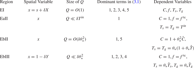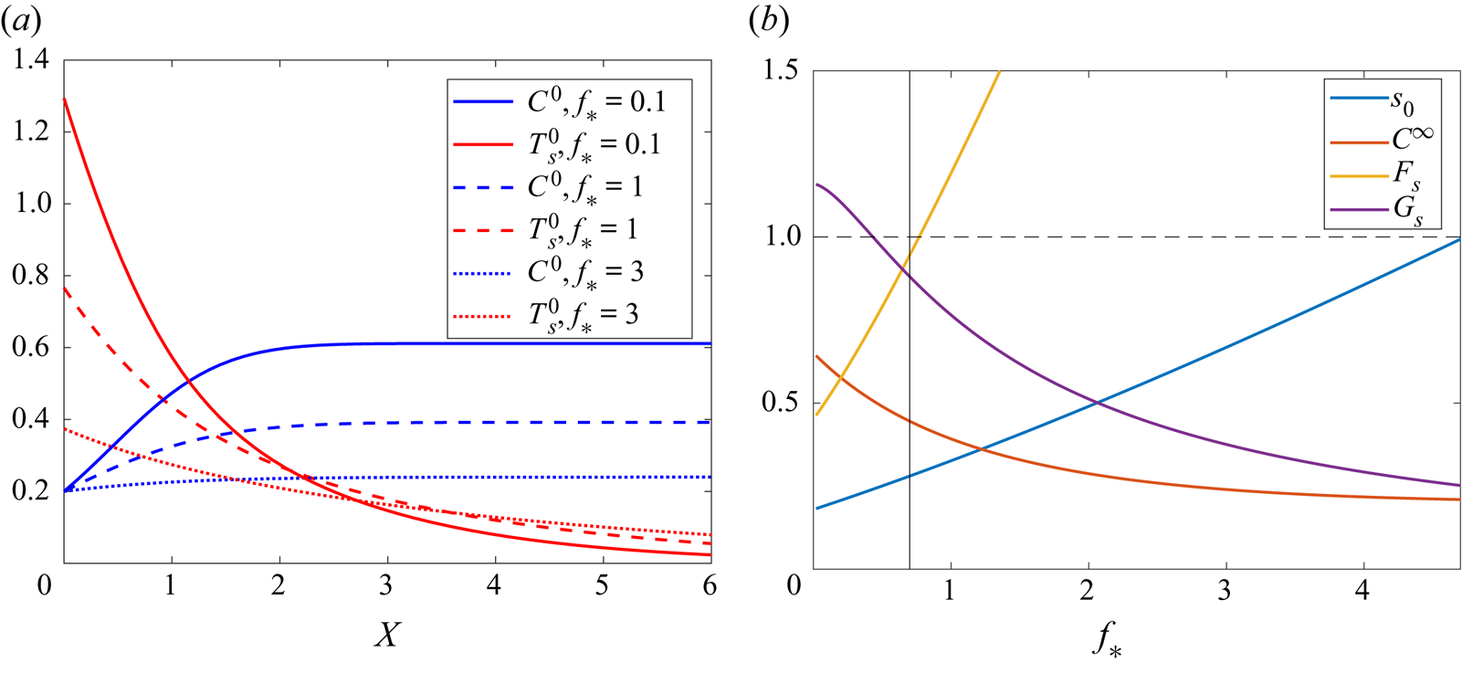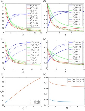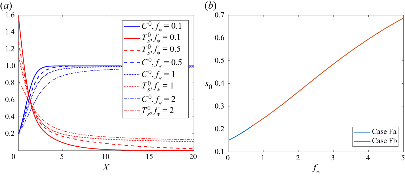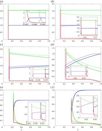

1. Introduction
Counter-current flows are systems in which two materials flow in opposite directions, meanwhile exchanging either heat or mass. Mass-exchanging counter-current flows are found in biological systems such as the production of urine in the kidneys (Winters & Davies Reference Winters and Davies1961), occur in oil extraction (Abd et al. Reference Abd, Elhafyan, Siddiqui, Alnoush, Blunt and Alyafei2019) and are ubiquitous in chromatography and the separation of chemicals (Sutherland Reference Sutherland2007; Brunner Reference Brunner2009; Ignatova et al. Reference Ignatova, Hewitson, Mathews and Sutherland2011; Skalicka-Woźniak & Garrard Reference Skalicka-Woźniak and Garrard2014). Heat-exchanging counter-current flows are also found in biology, including blood flow through the body (Mitchell & Myers Reference Mitchell and Myers1968) and in the respiratory system (Schmidt-Nielsen, Hainsworth & Murrish Reference Schmidt-Nielsen, Hainsworth and Murrish1970), and are used for efficient coolant systems, for instance in the nuclear industry (Deendarlianto, Lucas & Vierow Reference Deendarlianto, Lucas and Vierow2012).
We are interested in systems of heat-exchanging, counter-current flow, in which the heat transferred between the phases is necessary for an endothermic chemical reaction in the cooler phase, with temperature-dependent reaction rate. A classical counter-current heat-exchange system, modelling blood flow in the veins and arteries, is studied by Mitchell & Myers (Reference Mitchell and Myers1968), with the decay or growth of the temperatures in the two opposing flows found analytically as functions of distance. The key parameters are shown to be (i) the ratio of the heat-transfer rate between the veins and arteries to the flow rate of the blood, and (ii) the ratio of the heat-transfer rate with the external environment to the flow rate of the blood. Similar counter-current models are studied by Fitt, Ockendon & Shillor (Reference Fitt, Ockendon and Shillor1985), Hagan & Ockendon (Reference Hagan and Ockendon1991) and Nunge & Gill (Reference Nunge and Gill1965), although unlike Mitchell & Myers (Reference Mitchell and Myers1968), these take into account the diffusion processes at the interface between the fluids, rather than prescribing a bulk heat-transfer coefficient. These studies highlight one particular difficulty of analysing counter-current flows: since the models are forward/backward (or two-way) diffusion equations (Beals Reference Beals1981), care must be taken to ensure well-posedness. Eigenfunction methods on the half-range of the domain have been developed (Hagan & Ockendon Reference Hagan and Ockendon1991), and used to explore the efficiency of the counter-current system.
Although it is possible to find examples of reactive flows which are also counter-current flows, the literature in general neglects counter-current flows in the presence of chemical reactions. The interaction of fluid flow and heat transfer with chemical reactions is often studied in relation to combustion and flames (Tieszen Reference Tieszen2001). For non-pre-mixed combustion, a diffusive flame front is found at the interface between the two gaseous reactants (Bilger Reference Bilger1989). The effect of mixing at the flame front has been analysed in detail both for laminar (Sirignano Reference Sirignano2021) and turbulent (Bilger Reference Bilger1989) mixing layers. Flame fronts are also analysed in an applied counterflow (Ravikrishna & Sahu Reference Ravikrishna and Sahu2018), which allows for steady-state flame structures. Single-temperature combustion models are studied by Merzhanov & Khaikin (Reference Merzhanov and Khaikin1988), with the domain divided into reaction zones, and travelling flame fronts are found. Single-temperature models of counterflow filtration combustion are studied by Booty & Matkowsky (Reference Booty and Matkowsky1991), Chapiro & de Souza (Reference Chapiro and de Souza2016), Chapiro & Senos (Reference Chapiro and Senos2018) and Schult, Bayliss & Matkowsky (Reference Schult, Bayliss and Matkowsky1998). The existence and uniqueness of solutions to such systems is shown by Chapiro & Senos (Reference Chapiro and Senos2018), while Booty & Matkowsky (Reference Booty and Matkowsky1991), Chapiro & de Souza (Reference Chapiro and de Souza2016) and Schult et al. (Reference Schult, Bayliss and Matkowsky1998) find travelling-wave solutions asymptotically. Schult et al. (Reference Schult, Bayliss and Matkowsky1998) further characterise several types of instabilities of the travelling-wave solutions to the single-temperature model. In situations where not all chemicals are at the same temperature, the inter-phase heat transfer must be taken into account. For instance, the combustion of porous solids is also studied using two-temperature models, with applications to catalytic converters and filtration combustion (Norbury & Stuart Reference Norbury and Stuart1988; Byrne & Norbury Reference Byrne and Norbury1994, Reference Byrne and Norbury1997), smouldering cigarettes (Egerton, Gugan & Weinberg Reference Egerton, Gugan and Weinberg1963) and the combustion of rocket fuels (Koopmans et al. Reference Koopmans, Shrimpton, Roberts and Musker2013). Similarly to the single-temperature case, the reaction is found to take place in a hot reaction zone, which is shown to move as a travelling-wave flame front through the domain (Norbury & Stuart Reference Norbury and Stuart1988; Byrne & Norbury Reference Byrne and Norbury1997). The motion of flame fronts is studied by Please, Liu & McElwain (Reference Please, Liu and McElwain2003) for a system with a two-stage chemical reaction, the second of which may be endothermic. Under certain conditions on this endothermic reaction, travelling combustion waves with a similar structure to purely exothermic flame fronts are still found.
By contrast, in many metallurgical applications the chemical reactions of interest are endothermic, and heat-exchanging counter-current flows are used to provide energy for endothermic chemical reactions. For instance, the production of rutile titanium dioxide in a rotary kiln (Agrawal & Ghoshdastidar Reference Agrawal and Ghoshdastidar2017), the pyrolysis of aluminium (Marias, Roustan & Pichat Reference Marias, Roustan and Pichat2005), the production of cement (Spang Reference Spang III1972) and the production of silicon in a submerged arc furnace (Schei, Tuset & Tveit Reference Schei, Tuset and Tveit1998) all involve endothermic chemical processes in which heat required for the reaction is provided by a counter-current flow. In these endothermic processes, heat is removed from the system by the reactions. Furthermore, the endothermic reactions have temperature-dependent reaction rates, meaning that the heat lost from the system depends on the local temperature, further affecting the counter-current heat transfer. These effects fundamentally change the behaviour from the classical counter-current exchange studied by Mitchell & Myers (Reference Mitchell and Myers1968). For instance, it is observed by Agrawal & Ghoshdastidar (Reference Agrawal and Ghoshdastidar2017) that once the reactant reaches a critical temperature in the rotary kiln, the energy transferred to it by the counter-current flow is used for the chemical reaction, and the reactant remains at or close to this critical temperature. Similar behaviour is seen in cement production (Spang Reference Spang III1972; Mujumdar & Ranade Reference Mujumdar and Ranade2006; Stadler, Poland & Gallestey Reference Stadler, Poland and Gallestey2011), with distinct regions of the domain in which different chemical and heat-transfer processes are seen to dominate, and there are critical temperatures at which certain reactions become important. Many reacting counter-current flow systems may also be viewed as free-boundary problems, as there is often a finite region within which the reaction takes place, and this region moves both as material is fed in and reacted away. It is of practical importance to understand the required length of the reactor such that the reaction is completed by the end of the reactor, as the process will fail if the material is fed in too fast for the necessary reactions to take place within the length scale of the reactor. For instance, when designing a kiln for the production of rutile titanium dioxide, the ‘kiln length’ must be determined so that the chemical reactions have completed by the time the reactant material reaches the end of the kiln (Agrawal & Ghoshdastidar Reference Agrawal and Ghoshdastidar2017), else the process will fail. There is a similar free boundary at the edge of the reacting material bed within a silicon furnace, where the material collapses or drips into the craters which form beneath the electrodes in the furnace (Andresen Reference Andresen1995; Sloman, Please & Van Gorder Reference Sloman, Please and Van Gorder2020).
Research into these endothermic, reacting, counter-current flows in the literature is limited to numerical simulations of specific models for specific applications (Spang Reference Spang III1972; Mujumdar & Ranade Reference Mujumdar and Ranade2006; Stadler et al. Reference Stadler, Poland and Gallestey2011; Agrawal & Ghoshdastidar Reference Agrawal and Ghoshdastidar2017). We have highlighted above similar features of these flows that are observed across the different applications, specifically the distinct regions of the reactor in which the reaction occurs or not, the free-boundary nature of these problems, and the regions in which the reactant remains at a uniform, critical temperature while the endothermic reaction is taking place. It is not clear from these numerical studies, however, how the sizes of these distinct regions, the value of the critical temperatures or the position of the free boundaries depend on the flow rates, the heat transfer rate between the phases and the chemical reaction rates.
In this paper, we formulate a mathematical model for a generic endothermic, reacting, counter-current flow moving in one dimension, and then carry out a detailed asymptotic analysis to detect all distinguished limits as well as the size of all important length scales for each limit. Specifically, we consider the flow of a hot gas through a granular porous structure which is flowing slowly in the opposite direction. As the solid material is heated, it reacts to form the gas. The reaction is endothermic, with a temperature-dependent reaction rate. One direct application motivating our model is the production of silicon within a submerged arc furnace. In this application there are two sources of heat for the chemical reactions: the hot gases flowing through the material bed, and the heat radiation onto the free surface at the edge of the material bed. An asymptotic analysis of the endothermic reactions within a silicon furnace is provided by Sloman, Please & Van Gorder (Reference Sloman, Please and Van Gorder2018), but under the restrictive assumption that all chemical species have the same temperature locally, which precludes many of the counter-current flow effects.
Using the method of matched asymptotic expansions, we explore several distinguished limits corresponding to different heat-transfer rates between the two phases, spanning the whole range of this parameter. In many of these distinguished limits we find the same features observed in the other endothermic metallurgical systems, including the critical temperatures at which the reaction begins, and regions of uniform solid temperature. We show that these features arise at small or intermediate heat-transfer rates. We additionally characterise how these features depend on the flow rates, heat-transfer rates and the temperature dependence of the chemical reaction rate. By studying distinguished limits for large heat-transfer rates, we can also understand those parameter regimes for which our model reduces to a single-temperature model, providing a region of validity for single-temperature models such as that of Sloman et al. (Reference Sloman, Please and Van Gorder2018). The endothermic nature of the chemical reactions makes this system quite different to exothermic combustion processes, but there are also some similarities. Specifically, we find that the majority of the chemical reaction occurs within a hot reaction zone, analogous to the flame front in combustion processes, where the reaction rate is greatest. However, since the reaction is endothermic, this region is not self-sustaining, and is instead reliant on radiation at the boundary which provides heat that diffuses through the reaction zone. In this way, radiation at the boundary is rate limiting for the endothermic reaction.
The remainder of the paper is structured as follows. In § 2 we present our model for the coupled counter-current flow, heat transfer and endothermic chemical reaction system. In § 3 we give an overview of the asymptotic analysis, which is given in detail in §§ 4–9. We study asymptotic structures in a one-dimensional geometry, in the limit of large Péclet number in the solid material. In §§ 4–9, we identify the various distinguished limits for different sizes of the dimensionless convective heat-transfer coefficient (relative to the inverse Péclet number), ranging from it being negligible in § 4 to large in § 9. Numerical solutions of the reduced models are computed in § 10, and our composite asymptotic solutions are compared with numerical solutions of the full model in § 11. In § 12, we discuss our results and provide concluding remarks.
2. Model development
We model the counter-current process within the material bed of a silicon furnace using the framework of multiphase flow (see, for example, Brennen Reference Brennen2005). Our model is similar to that used by Luckins et al. (Reference Luckins, Oliver, Please, Sloman and Van Gorder2022), although we now include the heat transfer between the phases which is important on the longer domain length scale now considered.
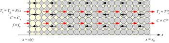
As well as the silicon furnace, many of the other metallurgical applications of interest consist of essentially one-dimensional flows, and we will restrict ourselves to a one-dimensional geometry in this paper. Specifically, we consider the one-dimensional domain  $x\in [s(t),x_0]$, where
 $x_0$ is prescribed and
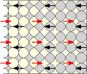
 $s(t)\in (0,x_0)$ is a free boundary, as illustrated in figure 1. We consider a two-phase flow within this domain, consisting of a granular solid material
 $s$ saturated with a connected gas phase
 $g$. We assume that solid material flows into the domain through the boundary
 $x=x_0$, and has velocity
 $\boldsymbol {u}_s=-u_s\boldsymbol {e}_x$. The gas phase flows in the opposite (positive-
 $x$) direction, with velocity
 $u_g\boldsymbol {e}_x$.
Schematic of the dimensional model domain  $x\in [s,x_0]$, with granular solid (grey) moving right-to-left as shown by the black arrows, surrounded by gas (pale yellow) flowing left-to-right as shown by the red arrows. The solid particles become smaller nearer to the free boundary
 $x=s(t)$, as solid mass is reacted away. The boundary conditions are shown at
 $x=s(t)$ and
 $x=x_0$.

The solid material reacts to form the gas at rate  $\tilde {Q}$ so that the conservation of mass of each phase is given by
 \begin{equation} \frac{\partial{\rho_g}}{\partial{t}}+\frac{\partial}{\partial x} (\rho_g u_g)=\tilde{Q}, \quad \frac{\partial{\rho_s}}{\partial{t}}+\frac{\partial}{\partial x}(-\rho_s u_s)={-}\tilde{Q}, \end{equation}
where  $\rho _N$ is the overall density within the mixture of phase
 $N=g,s$.
We assume that the reaction rate  $\tilde {Q}$ is an increasing function of the solid reactant temperature,
 $T_s$, as well as of the local density of solid material. We model this via an Arrhenius law of the form
 \begin{equation} \tilde{Q}=k_Q\rho_s\exp\left(-\frac{a_Q}{T_s}\right), \end{equation}
where  $k_Q$ (s
 $^{-1}$) is the rate constant and
 $a_Q$ (K) encodes the activation energy of the reaction. We do not assume a high-activation limit as is commonly done in the literature (Buckmaster & Ludford Reference Buckmaster and Ludford1983), but instead retain the form (2.2) in general.
As well as having a temperature-dependent reaction rate, the chemical reaction is assumed to be endothermic. Since it is the solid phase which is reacting, and since it is expected to have the higher thermal conductivity of the two phases, we assume that the heat energy  $\Delta H\tilde {Q}$ for the reaction is taken entirely from the solid phase. The equations of conservation of energy for both the gas and the solid phases are
 $$\begin{gather} \frac{\partial}{\partial t}\left(\rho_g c_{p,g}T_g\right)+\frac{\partial}{\partial x} \left(\rho_g c_{p,g}T_gu_g\right)={-}\lambda(T_g-T_s)+m, \end{gather}$$
 $$\begin{gather}\frac{\partial}{\partial t}\left(\rho_s c_{p,s}T_s\right)+\frac{\partial}{\partial x} \left(-\rho_s c_{p,s}T_s u_s\right)=\frac{\partial}{\partial x}\left(k_s\frac{\partial T_s}{\partial x}\right)-\Delta H \tilde{Q}+\lambda(T_g-T_s)-m, \end{gather}$$
where  $T_N$ is the temperature of phase
 $N$, and we assume for simplicity that the specific heat capacities
 $c_{p,N}$ of both the gas and solid phases are constant. Here,
 $m$ is the net heat gained by phase
 $g$ from phase
 $s$ due to the transfer of mass (by chemical reactions) between the two phases. We neglect heat diffusion in the gas phase, which is expected to be negligible in comparison with the advection of heat in this phase, but assume the granular solid material has constant, non-zero effective thermal conductivity
 $k_s$. We note that in the silicon furnace, some of this solid material is quartz rock. This quartz rock softens at high temperatures, becoming a very high viscosity liquid (Schei et al. Reference Schei, Tuset and Tveit1998; Luckins et al. Reference Luckins, Oliver, Please, Sloman and Van Gorder2022). As such, the contact points between the solid particles will actually have non-negligible surface area and so it is reasonable to expect heat conduction through the solid structure. The convective heat transfer between the phases is modelled to be linear in the temperature difference between the phases, with coefficient
 $\lambda$ (W m−3 K−-1). For two-phase flow, the convective heat-transfer coefficient
 $\lambda$ generally depends on the porosity, the porous structure, the relative velocity of the phases and the associated Reynolds number and Prandtl number of the flow (Brennen Reference Brennen2005; Kaviany Reference Kaviany2012). Estimates for
 $\lambda$ vary for different flow regimes and porous structures. The net heat transfer,
 $m$, due to the inter-phase transfer of mass depends on the temperature of both phases, the chemical reaction rate and the stoichiometry of the reaction – a discussion of these processes is given by Ni & Beckermann (Reference Ni and Beckermann1991), where
 $m$ is shown to depend on the interfacial temperature (at the interface between the two phases on the microscale). For simplicity, we assume that the heat content
 $c_{p,s}T_s$ of phase
 $s$ is carried with the material as it changes phase due to the chemical reaction, with rate equal to the rate of the reaction
 $\tilde {Q}$. This results in the form
 $m=c_{p,s}T_s\tilde {Q}$ which is also used by Baer & Nunziato (Reference Baer and Nunziato1986).
To close the model, we in general require the phase velocities  $u_s$ and
 $u_g$. In one dimension, the solid velocity may be fixed simply by a compaction law or a description of the compressibility of the solid matrix, without needing to study conservation of momentum directly. For simplicity, we assume that the solid matrix is incompressible. The resulting uni-directional solid velocity
 $u_s$ is thus constant. Since the density of the gas is so much less than the density of the solid, the velocity of the gas produced by the reaction must be many orders of magnitude larger than the solid velocity. Thus the gas phase may be assumed to be quasi-steady on the slow time scale of variation in the solid phase (see Luckins et al. (Reference Luckins, Oliver, Please, Sloman and Van Gorder2022) for a detailed dimensional analysis). In our one-dimensional geometry, the quasi-steady gas flow is fully described by the mass flux
 \begin{equation} f=\frac{\rho_gu_g}{M_g}, \end{equation}
and we need not deal directly with the gas velocity. We also change variables in order to consider the problem in terms of the solid concentration
 \begin{equation} C=\frac{\rho_s}{M_s}, \end{equation}
rather than the density. Since the solid is reacting to form the gas, in a reaction which we assume has stoichiometry 1, we note that the molar masses  $M:=M_s=M_g$ are equal.
Equations (2.1a,b) and (2.3) thus become a system for  $C$,
 $f$,
 $T_s$, and
 $T_g$, in
 $x\in [s(t),x_0]$, namely
 $$\begin{gather} \frac{\partial{C}}{\partial{t}}-u_s\frac{\partial{C}}{\partial{x}}={-}Q, \end{gather}$$
 $$\begin{gather}\frac{\partial{f}}{\partial{x}}=Q, \end{gather}$$
 $$\begin{gather}Mc_{p,s}C\left(\frac{\partial{T_s}}{\partial{t}}-u_s\frac{\partial{T_s}}{\partial{x}}\right)=k_s\frac{\partial{{}^{2}T_s}}{\partial{x^{2}}}+\lambda (T_g-T_s)-\Delta H MQ, \end{gather}$$
 $$\begin{gather}M c_{p,g}\frac{\partial}{\partial x}\left(fT_g\right)=Mc_{p,s}T_sQ-\lambda (T_g-T_s), \end{gather}$$
where the term  $m$ in the solid heat equation has been absorbed into the advection term on the left, using the equation of conservation of mass in the solid material. Here, we use the notation
 \begin{equation} Q=k_QC\exp\left(-\frac{a_Q}{T_s}\right), \end{equation}
for the chemical reaction rate in terms of the solid concentration.
2.1. Boundary and initial conditions
The equations of conservation of mass in the solid and gas phases (2.6a)–(2.6b) are both hyperbolic. We impose the inflowing concentration of solid at  $x=x_0$, and a flux of gas
 $f_*$ through the free boundary, so that
 \begin{equation} C=C^{in} \quad \text{at }x=x_0, \quad f=f_* \quad \text{at }x=s(t). \end{equation}
We prescribe a cold temperature of the inflowing solid material
 \begin{equation} T_s=T_s^{in} \quad \text{at }x=x_0. \end{equation}
At the free boundary, we impose
 \begin{equation} T_g=T_s=\frac{R}{s} \quad \text{at }x=s(t),\end{equation}
which is a crude model for a point radiative heat source at  $x=0$, with constant intensity
 $R$, incident on this boundary. This boundary condition is motivated by the electric arc which forms in the (roughly cylindrical) crater region within the material bed of a silicon submerged arc furnace (Schei et al. Reference Schei, Tuset and Tveit1998). For other applications, different forms for the boundary condition (2.8c) may be more appropriate.
The position of the free boundary  $x=s(t)$ is determined by the Stefan-like condition on the concentration of solid material
 \begin{equation} C=C_* \quad \text{at }x=s(t), \end{equation}
where  $C_*< C^{in}$. Thus the free boundary of the domain is the position where sufficient solid material has been reacted away. For silicon furnaces, this condition describes the position of the edge of the gas-filled crater that forms deep within the furnace:
 $C_*$ is the critical concentration at which the solid structure loses structural integrity, and any remaining solid material collapses into the crater.
Finally, we require an initial configuration for the system as initial conditions on  $C$,
 $f$,
 $T_s$,
 $T_g$ and the position
 $s$ of the free boundary. These initial conditions must be consistent with the boundary conditions described above.
2.2. Non-dimensionalisation
We non-dimensionalise the model (2.6) and (2.8) by scaling  $x=x_0 x'$,
 $s=x_0 s',$
 $t=x_0t'/u_s,$
 $C=C^{in}C',$
 $f=[f]f',$
 $T_s=[T_s]T_s'$ and
 $T_g=[T_g]T_g'$, where the prime notation denotes dimensionless variables. The temperature scalings are given by the boundary condition at
 $x=s(t)$, since this is the major source of heat to the system, and so we fix
 $[T_s]=[T_g]=R/[s],$ where
 $[s]$, to be determined, is the expected size of
 $s$. We define
 $\delta$ to be the inverse Péclet number
 \begin{equation} \delta=Pe^{{-}1}=\frac{k_s}{x_0u_sMc_{p,s}C^{in}}. \end{equation}
Throughout this paper we assume that  $\delta$ is small, so that the effective thermal conductivity of the porous solid structure is small over the relatively large length scale of the domain. Thus the heat provided to the solid material at the boundary
 $x=s(t)$ cannot penetrate far into the domain: we anticipate a conductive boundary layer at this boundary, of width
 $O(\delta )$.
Assuming that the majority of the chemical reaction occurs in this hot  $O(\delta )$ boundary layer at
 $x=s(t)$, the length scale
 $[s]$ is given by a balance in the solid mass equation (2.6a),
 \begin{equation} \frac{u_s}{\delta x_0}=k_{Q}\exp\left(\frac{-a_Q[s]}{R}\right), \end{equation}
which, along with the definition of  $\delta$, gives
 $[s]=(R/a_Q)\log (k_{Q}k_s/(Mc_{p,s}u_s^{2}C^{in})).$ The temperature scalings are therefore
 $[T_s]=[T_g]=a_Q/\log (k_Qk_s/(Mc_{p,s}u_s^{2} C^{in})).$ We note that for these temperature scalings to be positive, the velocity
 $u_s$ of the solid material must be sufficiently small. Specifically, we require
 \begin{equation} u_s<\sqrt{\frac{k_Qk_s}{Mc_{p,s}C^{in}}}. \end{equation}
For larger  $u_s$ than this, the (bounded) Arrhenius chemical reaction rate cannot match the rate at which material flows in, and the model ceases to be valid. Finally, balancing the gas mass equation (2.6b) requires
 $[f]=u_sC^{in}$.
With these scalings, and dropping the prime notation, the equations become
 $$\begin{gather} \delta\left(\frac{\partial{C}}{\partial{t}}-\frac{\partial{C}}{\partial{x}}\right)={-}Q, \end{gather}$$
 $$\begin{gather}\delta\frac{\partial{f}}{\partial{x}}=Q, \end{gather}$$
 $$\begin{gather}C\left(\frac{\partial{T_s}}{\partial{t}}-\frac{\partial{T_s}}{\partial{x}}\right)=\delta\frac{\partial{{}^{2}T_s}}{\partial{x^{2}}}+\mu(T_g-T_s)-\frac{\gamma}{\delta} Q, \end{gather}$$
 $$\begin{gather}K\frac{\partial}{\partial x}(fT_g)=\frac{1}{\delta}T_sQ-\mu(T_g-T_s), \end{gather}$$
on the domain  $x\in (s(t),1)$, where the dimensionless chemical reaction rate is
 \begin{equation} Q(C,T_s)=C\exp\left(A\left(1-\frac{1}{T_s}\right)\right), \end{equation}
and with boundary conditions
 $$\begin{gather} C=C_*,\quad f=f_*, \quad T_s=T_g=\frac{\rho}{s} \quad \text{at }x=s(t), \end{gather}$$
 $$\begin{gather}C=1,\quad T_s=T^{in} \quad \text{at }x=1, \end{gather}$$
with  $f_*,C_*$ and
 $T^{in}$ appropriately rescaled.
Here, we have introduced the dimensionless parameters
 \begin{equation} A=\frac{a_Q[s]}{R}, \quad \mu=\frac{\lambda x_0}{u_sMc_{p,s}C^{in}}, \quad K=\frac{c_{p,g}}{c_{p,s}}, \quad \gamma=\frac{[s]\Delta H}{Mc_{p,s}R}, \quad \rho=\frac{[s]}{x_0}. \end{equation}
In addition to (2.12), we require initial conditions for  $C$,
 $f$,
 $T_g$,
 $T_s$ and
 $s$. The system (2.12) is a fifth-order system of differential equations in space, with an additional degree of freedom in the position
 $s$ of the free boundary. We therefore expect the model to be correctly specified since we impose six boundary conditions.
Throughout, we assume that the dimensionless parameters  $K,$
 $\gamma,$
 $A,$
 $\rho$,
 $C_*$ and
 $f_*$ in the model (2.12) are of order unity (see Luckins et al. (Reference Luckins, Oliver, Please, Sloman and Van Gorder2022) for justification in the case of a silicon furnace). The inverse Péclet number,
 $\delta$, is expected to be of the order of
 $10^{-3}-10^{-2}$ (Luckins et al. Reference Luckins, Oliver, Please, Sloman and Van Gorder2022), and is the smallest parameter in the system. The asymptotic analysis in this paper is in the limit of
 $\delta \rightarrow 0$. We also assume that the input temperature of the solid,
 $T^{in}$, is small. Specifically, we require
 \begin{equation} \delta T^{in}\gg \exp\left(A\left(1-\frac{1}{T^{in}}\right)\right), \end{equation}
so that the rate of reaction at this temperature is much less than the rate at which material moves through the whole domain by advection. Thus, if there were no heating, we would expect the solid material not to appreciably react away over the time it spends moving through the domain. We further assume that  $\delta \ll T^{in}$, meaning that, although
 $T^{in}$ is small in the sense of (2.14), it is not as small as
 $\delta$. This further assumption that
 $\delta \ll T^{in}$ does not impact the dominant behaviour of the system, and is only needed when analysing the correction terms to the leading-order behaviour in certain parameter regimes. The final dimensionless parameter is
 $\mu$, which encodes the rate of convective heat transfer between the phases. We will explore various distinguished limits relating
 $\mu$ to
 $\delta$.
3. Overview of asymptotic analysis
In §§ 4–9, we will consider a range of different distinguished limits corresponding to different values of the convective heat-transfer coefficient  $\mu$, in terms of functions of
 $\delta$. We refer to these distinguished limits as cases A–F, studied in §§ 4–9, respectively, in order of increasing
 $\mu$, with case A being the small-
 $\mu$ limit,
 $\mu \rightarrow 0$ (which we show is valid for
 $\mu \ll 1/\log (1/\delta )$), and case F the large-
 $\mu$ limit (corresponding to
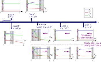
 $\mu \gg \delta ^{-1}$). A schematic of the solution structures in each of the cases A–F is shown in figure 2. Detailed schematics are given for each case in §§ 4–9.
Schematics of the different asymptotic solution structures (in steady state for cases D–F) for increasing  $\mu$. In each case, the solutions,
 $T_s$ (red curves),
 $T_g$ (green curves) and
 $C$ (blue curves) are illustrated in the domain
 $x\in [s(t),1]$, with boundary layers and transition layers shown by the grey regions.

The asymptotic results that we present in this paper are mostly determined by the various dominant balances in the equation of conservation of energy in the solid, (2.12c). We label the terms in this equation as follows:
 \begin{equation} \underbrace{C\left(\frac{\partial{T_s}}{\partial{t}}-\frac{\partial{T_s}}{\partial{x}}\right)}_1=\underbrace{\delta\frac{\partial{{}^{2}T_s}}{\partial{x^{2}}}}_2+\underbrace{\mu(T_g}_3-\underbrace{T_s)}_4-\underbrace{\frac{\gamma}{\delta} C\exp\left(A\left(1-\frac{1}{T_s}\right)\right)}_5,\end{equation}
for explicit reference in our analysis. Terms 1 and 2 describe the advection and conduction, respectively, of heat within the solid material. Terms 3 and 4 describe the heat transferred to the solid by the gas, and are labelled separately since  $T_s$ and
 $T_g$ may have different sizes in different regions of the domain. Term 5 is the heat absorbed by the endothermic chemical reaction.
Since  $\delta \ll 1$, heat conduction in the solid material (term 2 in (3.1)), has negligible effect through most of the domain. However, for all sizes of the convective heat-transfer coefficient
 $\mu$, we will find a boundary layer of width
 $O(\delta )$ at
 $x=s(t)$, in which heat conduction (term 2) is important. It is only in this thin layer that the heating of the solid material from the radiation incident onto the boundary as in (2.12 f) is felt. This boundary layer is the region of largest
 $T_s$ in the domain: in all other regions we will find
 $T_s\ll 1$. Since the chemical reaction rate is temperature dependent, the most intense material consumption also therefore occurs in this
 $O(\delta )$ boundary layer at
 $x=s(t)$. Region I is therefore interpreted as the fast reaction region, with the heat of reaction provided by the radiation at the boundary. In all cases A–F, the reduced model in this boundary layer determines the position
 $s(t)$ of the free boundary. For some moderate values of
 $\mu$ the behaviour in the outer regions is coupled to the boundary-layer problem at leading order, and so also affects the position
 $s$.
Outside of this boundary layer there can be several types of behaviour depending on the size of the convective heat-transfer coefficient  $\mu$. For small
 $\mu$ (case A), very little happens outside the boundary layer, with the solid temperature simply equal to its input value
 $T_s=T^{in}$ at leading order. For moderate
 $\mu$ (cases B–D), there is a balance between the transfer of heat from the gas to the solid (term 3 in (3.1)), and the energy consumed by the chemical reaction (term 5). In these cases, this balance determines the natural solid temperature scaling
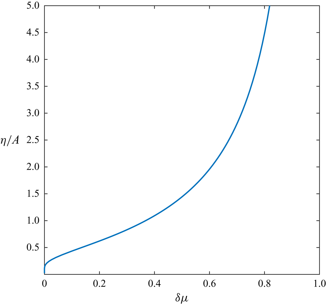
 \begin{equation} \eta:=\frac{A}{\log\left(\dfrac{1}{\delta\mu}\right)},\end{equation}
and we find that  $T_s\approx \eta$ is uniform throughout such regions of the domain. Since
 $\eta$ depends on
 $\mu$, for the different sizes of
 $\mu$ in cases B–D the value of
 $\eta$ is different. The ratio
 $\eta /A$ is plotted as a function of
 $\delta \mu$ in figure 3. We note that
 $\eta$ is monotone increasing in
 $\delta \mu$, with
 $\eta \rightarrow 0$ as
 $\delta \mu \rightarrow 0$, and that
 $\eta$ blows up as
 $\delta \mu \rightarrow 1$. In all cases B–D we have
 $\delta \mu \ll 1$, so that
 $\eta \ll 1$ is small, although due to the logarithmic form of
 $\eta$, we have
 $\delta \ll \eta$.
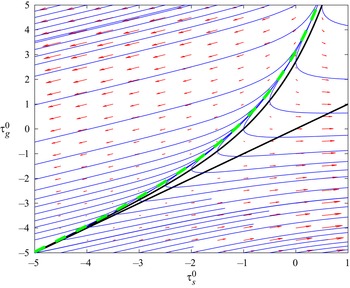
The variation of  $\eta /A$ with
 $\delta \mu$, according to (3.2). The curve approaches the origin as
 $\delta \mu \rightarrow 0$, and becomes unbounded as
 $\delta \mu \rightarrow 1$.

For large  $\mu$ (cases D–F), we find that the heat transfer between phases, terms 3 and 4, dominate at leading order over an
 $O(1)$ length scale, so that we obtain a single-temperature model in the outer region of the domain. By combining the equations of conservation of energy for the gas and solid phases, we derive a single equation for the common, leading-order temperature
 $T_s=T_g=T$ in the
 $O(1)$-length scale regions of the domain. We observe interesting counter-current behaviour in these cases D–F: since the gas and solid material flow in opposite directions, the net direction of advection for the common temperature
 $T$ may be in either direction, and the dominant behaviour is different in either case. In particular, if the net heat flow is left-to-right (with the gas flow) then the natural temperature scaling of the steady-state case is determined by a balance of advection, term 1, and heat consumed by the chemical reaction, term 5, giving the temperature scaling
 $\theta _*$, the solution of
 \begin{equation} \delta\theta_*^{2}=\exp\left(-\frac{A}{\theta_*}\right). \end{equation}
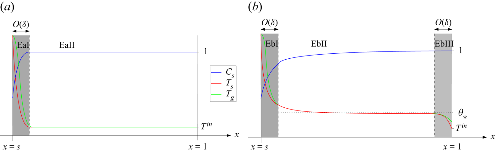
Conversely, if the net heat flow is right-to-left with the solid, the temperature remains approximately uniform at the solid input temperature  $T^{in}$. These are referred to as the subcases b and a respectively.
The asymptotic structures that we derive in cases B and C, characterised by the balance of heat transfer between the phases and material consumption over an  $O(1)$ length scale, are quite different to the single-temperature behaviour of cases E and F. The analysis in case D includes aspects of both these types of behaviour, and so demonstrates how the system varies from case C to E as the convective heat-transfer coefficient is increased.
In each of the cases considered in §§ 4–9 below, we find explicit steady-state solutions at leading order, in every region of the domain except the boundary layer at  $x=s(t)$. We construct composite, leading-order solutions in each case (restricting to steady state in cases D–F for simplicity).
4. Case A:  $\mu =0$, no heat transfer

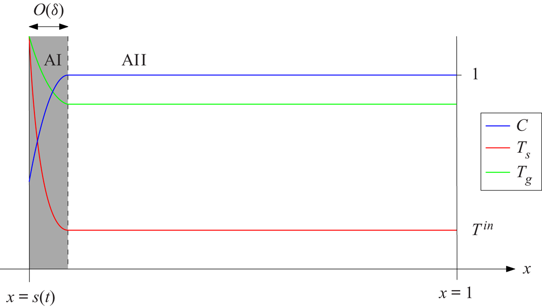
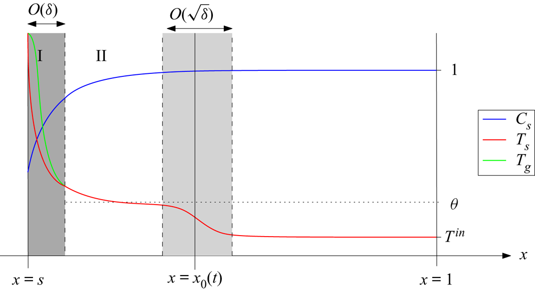
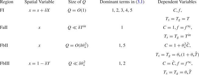
Firstly, we suppose that the heat transfer between the gas and solid phases is negligible over the length scale of the entire domain, so that  $\mu \rightarrow 0$. The diagram in figure 4 is a schematic of the asymptotic structure in this case, and the changes of variable that we will make in each region of the domain are summarised in table 1. As in figure 4, throughout this paper we number the regions of the domain with roman numerals I, II etc. from left-to-right within the domain.
Schematic of the solution structure in case A:  $\mu =0$.

Summary of the asymptotic regions of the domain, and the changes of variable in these regions, for case A:  $\mu =0$.

Since the convective heat-transfer coefficient is zero, the gas problem decouples from the solid problem, and we may study the reduced problem for the solid variables only. This is, for  $x\in (s(t),1)$, (2.12a) and (2.12c) (with
 $\mu =0$) and the boundary conditions for
 $C$ and
 $T_s$ as in (2.12g)–(2.12 f). We may then integrate (2.12b) and (2.12d), using the boundary conditions for
 $f$ and
 $T_g$ at
 $x=s(t)$ given by (2.12 f). This gives the gas variables
 $f$ and
 $T_g$ in terms of the solution
 $s$,
 $C$ and
 $T_s$ of the solid problem
 $$\begin{gather} f=f_*+\delta^{{-}1}\int_{x=s}^{1}C\exp\left(A\left(1-\frac{1}{T_s}\right)\right)\,\mathrm{d} x, \end{gather}$$
 $$\begin{gather}T_g=\frac{f_*T_s|_{x=s}+(\delta K)^{{-}1}\int_{x=s}^{1}T_sC\exp\left(A\left(1-\dfrac{1}{T_s}\right)\right)\,\mathrm{d} x}{f_*+\delta^{{-}1}\int_{x=s}^{1}C\exp\left(A\left(1-\dfrac{1}{T_s}\right)\right)\,\mathrm{d} x}. \end{gather}$$
We will see in the following analysis that the integral terms in (4.1) are  $O(\delta )$, and so
 $f$ and
 $T_g$ are regular as
 $\delta \rightarrow 0$.
4.1. Region AII
We begin by considering the behaviour over an  $O(1)$ length scale, which we denote region AII in figure 4. We recall that
 $T^{in}\ll 1$ is small, in the specific sense (2.14). At the boundary
 $x=1$ we have
 $T_s= T^{in}$, and we therefore look for a solution expansion of the form
 \begin{equation} T_s=T^{in}\left(\hat{T}^{0}_s+o\left(T^{in}\right)\right), \quad C=\hat{C}^{0}+o\left(T^{in}\right), \end{equation}
and also expand the gas variables in region AII by
 \begin{equation} T_g=\hat{T}^{0}_g+o\left(T^{in}\right), \quad f=\hat{f}^{0}+o\left(T^{in}\right). \end{equation}
(Here, we use hat notation to differentiate from the variables used in region AI below.) Since by (2.14) we have that  $Q(T^{in})\ll \delta T^{in}$, at leading order in (2.12a) and (2.12c) we obtain
 \begin{equation} \frac{\partial{\hat{C}^{0}}}{\partial{t}}-\frac{\partial{\hat{C}^{0}}}{\partial{x}}=0, \quad \hat{C}^{0}\left(\frac{\partial{\hat{T}_s^{0}}}{\partial{t}}-\frac{\partial{\hat{T}^{0}_s}}{\partial{x}}\right)=0. \end{equation}
Solving, using the boundary conditions at  $x=1$, we must have, for all
 $x$
 \begin{equation} \hat{T}_s^{0}=1, \quad \hat{C}^{0}=1. \end{equation}
Since  $\hat {T}_s$ and
 $\hat {C}$ are constant to leading order, the gas variables in this region, given by (4.1), are also uniform. The error in these leading-order solutions is
 $O(\delta ^{-1}Q(T^{in}))=o(T^{in})$, since
 $Q\ll \delta T^{in}$.
4.2. Region AI
We note that we cannot impose the boundary conditions at the free boundary  $x=s(t)$ on the constant solution found in the previous section. We therefore look for a boundary layer at
 $x=s(t)$, denoted region AI, where
 $T_s=O(1)\gg T^{in}$. Since
 $\delta \ll 1$, we change variables, setting
 $x=s(t)+\delta X$. Since
 $T^{in}\gg \delta$, we look for an expansion in powers of
 $T^{in}$ in region AI, setting
 \begin{align} T_s=T_s^{0}(X,t)+O\left(T^{in}\right), \quad C=C^{0}(X,t)+O\left(T^{in}\right), \quad s=s^{0}(t)+O\left(T^{in}\right). \end{align}
We also expand the gas variables in powers of  $T^{in}$, taking
 \begin{equation} T_g=T_g^{0}(X,t)+O\left(T^{in}\right), \quad f=f^{0}(X,t)+O\left(T^{in}\right). \end{equation}
Substituting the expansions (4.6a–c) into (2.12a) and (2.12c), at leading order we obtain
 $$\begin{gather} -\left(\dot{s}_0+1\right)\frac{\partial{C^{0}}}{\partial{X}}={-}C^{0}\exp\left(A\left(1-\frac{1}{T_s^{0}}\right)\right), \end{gather}$$
 $$\begin{gather}-\left(\dot{s}_0+1\right)C^{0}\frac{\partial{T_s^{0}}}{\partial{X}}=\frac{\partial{{}^{2}T_s^{0}}}{\partial{X^{2}}}-\gamma C^{0}\exp\left(A\left(1-\frac{1}{T_s^{0}}\right)\right), \end{gather}$$
where the dot notation denotes a time derivative,  $\dot {s}_0=\mathrm {d} s_0/\mathrm {d}t$. From (2.12 f), we have the boundary conditions
 \begin{equation} C^{0}=C_*, \quad T_s^{0}=\frac{\rho}{s_0}, \quad \text{at }X=0.\end{equation}
As  $X\rightarrow \infty$ we match with the outer region AII, and so require
 \begin{equation} C^{0}\rightarrow 1, \quad T_s^{0}\rightarrow 0 \quad \text{as}\ X\rightarrow\infty.\end{equation}
The far-field temperature must approach zero in (4.8d) so that the chemical reaction rate  $Q$ approaches zero in this limit. This is necessary for the problem to be correctly specified. Region AI is the reaction region, with the energy for the reaction provided by the heat radiation on the boundary
 $x=s(t)$. This reduced system (4.8) in region AI determines
 $T_s^{0}$,
 $C^{0}$ and also gives a relation between
 $\dot {s}_0$ and
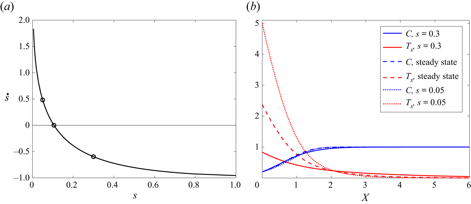
 $s_0$. We solve (4.8) numerically in § 10 below. We note that the leading-order system (4.8) is quasi-steady, in that the only time derivatives are
 $\dot {s}_0$, with no time derivatives of
 $T_s$ or
 $C_s$ at leading order. Since the region-AII problem has a constant, time-independent solution, we see that the entire system is quasi-steady in case A. The relation between
 $\dot {s}_0$ and
 $s_0$ found numerically as part of the solution of (4.8) in § 10 therefore describes fully the quasi-steady time-dependent behaviour of the system. In particular we may find steady state(s) of the system for which
 $\dot {s}=0$.
In fact, we obtain a quasi-steady boundary-layer problem, similar to (4.8), in each of the non-zero  $\mu$ cases explored below. In cases with larger
 $\mu$, however, we will find fully time-dependent behaviour outside of region I, so that, even though the region-I behaviour is still quasi-steady, the overall system is not quasi-steady. In the analysis of many of these cases we find and discuss the time-dependent solutions, but when computing solutions numerically in §§ 10–11 we will restrict ourselves to the steady-state case, for simplicity.
Given the solution of this solid problem (4.8), from (4.1) with the change of variables  $x=s(t)+\delta X$, we see that the leading-order gas variables in region AI are
 $$\begin{gather} f^{0}(X,t)=f_*+(1+\dot{s}_0)(C^{0}-C_*), \end{gather}$$
 $$\begin{gather}T_g^{0}(X,t)=\frac{\dfrac{f_*\rho}{s_0}+K^{{-}1}\int_{\bar{X}=0}^{X} T_s^{0}C^{0}\exp\left(A\left(1-\dfrac{1}{T^{0}_s}\right)\right)\,\mathrm{d}\bar{X}}{f_*+(1+\dot{s}_0)(C^{0}-C_*)}. \end{gather}$$
In region AII both  $\hat {T}_g^{0}$ and
 $\hat {f}^{0}$ are uniform. By matching with region AI at
 $x=s_0$, we find
 $$\begin{gather} \hat{f}^{0}(t)=F_s(t):=f_*+(1+\dot{s}_0)(1-C_*), \end{gather}$$
 $$\begin{gather}\hat{T}_g^{0}(t)=G_s(t):=\frac{\dfrac{f_*\rho}{s_0}+K^{{-}1}\int_{\bar{X}=0}^{\infty} T_s^{0}C^{0}\exp\left(A\left(1-\dfrac{1}{T^{0}_s}\right)\right)\,\mathrm{d}\bar{X}}{f_*+(1+\dot{s}_0)(1-C_*)}. \end{gather}$$
4.3. Composite solution
We construct composite leading-order solutions for case A as follows. Since  $C$,
 $f$ and
 $T_g$ are
 $O(1)$ in all regions of the domain, and uniform to leading order in region AII, the leading-order composite solutions in case A (which we denote by superscript A) are simply
 \begin{equation} C^{A}=C^{0}\left(\frac{x-s_0(t)}{\delta},t\right), \quad f^{A}=f^{0}\left(\frac{x-s_0(t)}{\delta},t\right), \quad T_g^{A}=T_g^{0}\left(\frac{x-s_0(t)}{\delta},t\right). \end{equation}
However,  $T_s$ is
 $O(1)$ in region AI, but
 $O(T^{in})$ in region AII. We note that this small temperature in region AII must induce a
 $O(T^{in})$ switchback correction (Hinch Reference Hinch1991) to the leading-order solution in the boundary layer AI. We therefore have some freedom in how to choose the leading-order composite expansion (Hinch Reference Hinch1991). For simplicity we choose to set the
 $O(T^{in})$ correction in region AI to be uniform, and equal to
 $T^{in}$. Thus we form the composite expansion
 \begin{equation} T_s^{A}=T_s^{0}\left(\frac{x-s_0(t)}{\delta}\right)+T^{in}, \end{equation}
which has  $O(T^{in})$ error in region AI, and
 $O(\delta ^{-1}Q(T^{in}))$ error in region AII.
In case A, we have seen that all the material consumption (chemical reaction) occurs within the boundary layer AI at  $x=s(t)$, and that all variables have constant, uniform profiles in the outer region AII. We also observed that the leading-order behaviour is quasi-steady throughout the domain, with the time-derivatives of
 $s$ in region AI the only time derivatives in the reduced problem.
5. Case B: $\mu =O(\eta )$, small heat transfer

We now let  $\mu >0$, and study the distinguished limit
 $\mu =O(\eta )$, with
 $\eta$ defined in (3.2). We will see that for this rate of heat transfer between phases, the solid temperature in the outer region of the domain becomes high enough for the chemical reaction to be non-negligible. In this section, we write
 $\mu =M\eta _B\ll 1$, where
 $M=O(1)$ and
 $\eta _B=\eta _B(\delta,A)$ is the smaller non-trivial solution of
 \begin{equation} \eta_B=\frac{A}{\log\left(\dfrac{1}{\delta\eta_B}\right)}, \end{equation}
namely
 \begin{equation} \eta_B=\frac{1}{\delta}\exp(W_{{-}1}({-}A\delta))=\frac{A}{-\log(A\delta)}\left(1+O\left(\frac{\log(-\log(A\delta))}{-\log(A\delta)}\right)\right), \end{equation}
where  $W_{-1}$ is the lower real branch of the Lambert W function. We note that
 $\eta _B\rightarrow 0$ as
 $\delta \rightarrow 0$. In this section, we will expand our dependent variables in powers of
 $\eta _B$ (rather than in powers of
 $T^{in}$ as in case A), but to leading order this is equivalent to expanding in powers of
 $1/-\log (A\delta )$. We choose to retain the
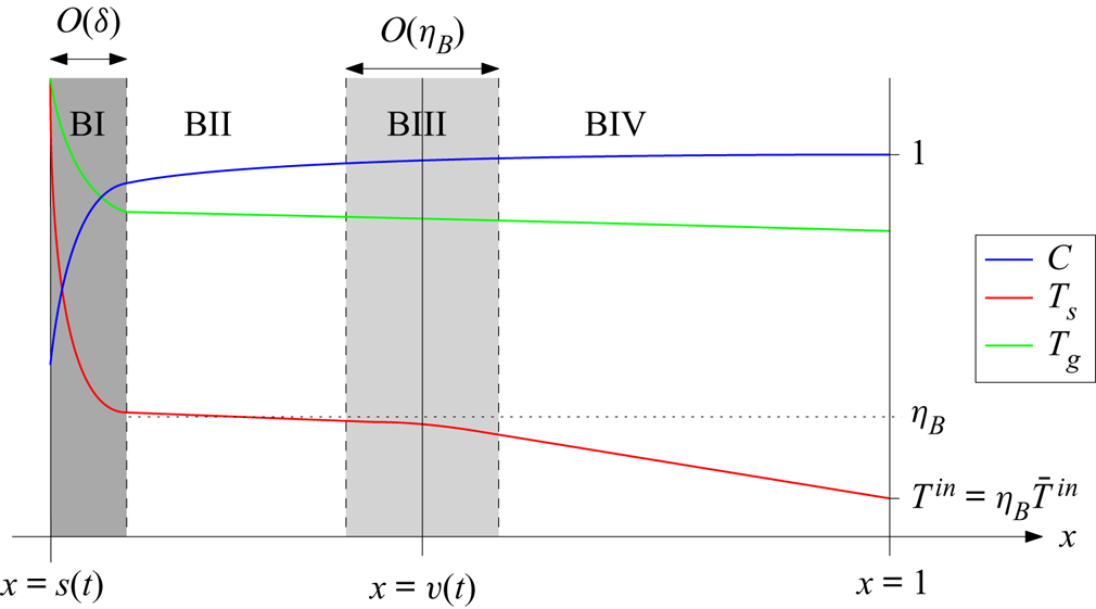
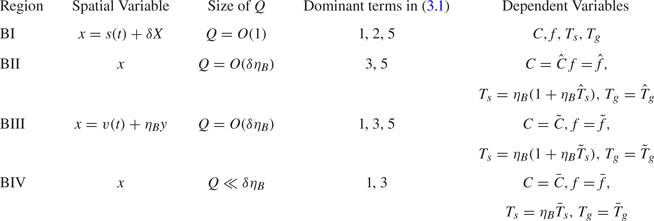
 $\eta _B$ notation as it makes for easy comparison with subsequent cases. A schematic of the asymptotic structure in case B is shown in figure 5, and the changes of variable are summarised table 2.
Schematic of the solution structure in case B:  $\mu =O(\eta _B)$.

Summary of the asymptotic regions of the domain, and the changes of variable in these regions, for case B:  $\mu =O(\eta _B)$.

5.1. Region BI
As in case A, we look for a reaction region at the free boundary  $x=s(t)$. This is an
 $O(\delta )$ boundary layer at
 $x=s(t)$, denoted region BI in figure 5. We look for an expansion solution in powers of
 $\eta _B$ in region BI, namely
 $$\begin{gather} T_s=T_s^{0}(X,t)+\eta_BT_s^{1}(X,t)+O\left(\eta_B^{2}\right), \quad C=C^{0}(X,t)+\eta_BC^{1}(X,t)+O\left(\eta_B^{2}\right), \end{gather}$$
 $$\begin{gather}T_g=T_g^{0}(X,t)+\eta_BT_g^{1}(X,t)+O\left(\eta_B^{2}\right), \quad f=f^{0}(X,t)+\eta_Bf^{1}(X,t)+O\left(\eta_B^{2}\right), \end{gather}$$
 $$\begin{gather}s=s_0(t)+\eta_Bs_1(t)+O\left(\eta_B^{2}\right). \end{gather}$$
Substituting into (2.12), (2.12b) and (2.12d) for the gas variables decouple on this length scale, and so we obtain exactly the same system at leading order for just the solid variables  $T_s^{0}$,
 $C^{0}$ and
 $s_0$ as in case A, namely (4.8). We will find below that
 $C=1+O(\eta _B)$ everywhere outside of region BI, and so the matching conditions as
 $X\rightarrow \infty$ are also identical to case A, given by (4.8d).
5.2. Region BII
Since the convective heat-transfer rate is non-zero, unlike case A, the equations for the gas variables do not decouple in (2.12) in the entire domain. Instead, outside the boundary layer BI, we must have heat transfer between the solid and gas phases, and expect the solid temperature scaling  $T_s\approx \eta _B$. We therefore make the rescaling
 \begin{equation} T_s=\eta_B\left(1+\eta_B\hat{T}_s\right), \end{equation}
in the  $O(1)$-length scale outer region, denoted region BII, and for clarity of notation we also write
 $C=\hat {C},$
 $f=\hat {f}$ and
 $T_g=\hat {T}_g$. The chemical reaction rate here is therefore
 \begin{equation} \hat{Q}(\hat{C},\hat{T}_s)=\hat{C}\exp\left(A\left(1-\frac{1}{T_s}\right)\right)=\hat{C}e^{A}\delta\eta_B\left(e^{A\hat{T}_s}+O(\eta_B)\right), \end{equation}
and thus the heat consumed by the chemical reaction at this temperature  $\eta _B$ is the same order (
 $\delta \eta _B$) as the heat transferred from the gas to the solid. We expand all dependent variables in powers of
 $\eta _B\ll 1$, setting
 \begin{equation} \left. \begin{aligned} \hat{T}_s & =\hat{T}_s^{0}(x,t)+O(\eta_B), \quad \hat{C}=\hat{C}^{0}(x,t)+O(\eta_B),\\ \hat{T}_g & =\hat{T}_g^{0}(x,t)+O(\eta_B), \quad \hat{f}=\hat{f}^{0}(x,t)+O(\eta_B). \end{aligned} \right\} \end{equation}
Since the reaction rate is small, at leading order we find that  $\hat {f}^{0}$ and
 $\hat {T}_g^{0}$ are uniform in
 $x$. Matching at
 $x=s(t)$ with region BI, using the same notation as in (4.10), we find
 \begin{equation} \hat{f}^{0}=F_s, \quad \hat{T}_g^{0}=G_s. \end{equation}
From (2.12a) we find that  $\hat {C}^{0}$ is conserved along characteristics travelling right-to-left through region BII. As we will see below,
 $C$ is uniform to leading order over all regions to the right of this, and so by using the boundary condition at
 $x=1$, and matching, we will find that
 $\hat {C}^{0}=1$ is constant throughout region BII. The solid heat equation (2.12c), at leading order (order
 $\eta _B$), reduces to
 \begin{equation} M\hat{T}_g^{0}=\gamma \hat{C}^{0}\exp\left(A(1+\hat{T}_s^{0})\right), \end{equation}
so that  $\hat {T}_s^{0}$ is also uniform, and given by
 \begin{equation} \hat{T}_s^{0}=\frac{1}{A}\log\left(\frac{MG_s}{\gamma}\right)-1. \end{equation}
This completes the leading-order analysis in region BII. Physically, in this region all the heat transferred from the gas to the solid is used for the chemical reaction, so that the solid temperature remains uniform. Region BII is a reaction region (like region BI), although here the heat for the chemical reaction is provided by the heat transfer between phases, rather than the radiation onto the free boundary.
5.3. Region BIV
For this size of the convective heat-transfer coefficient  $\mu =O(\eta _B)$, there is also a second possible dominant balance on an
 $O(1)$ length scale, namely the balance of advection (term 1 in (3.1)) with the heat transfer from the gas (term 3 in (3.1)), when the chemical reaction rate is small
 $Q\ll \delta \eta _B$. We see that this balance occurs at the right-hand side of the domain (denoted region BIV) since, near the boundary
 $x=1$,
 $T_s\approx T^{in}$, and we note that
 $\eta _B>T^{in}$, by the assumption (2.14). In region BIV, the solid material is therefore heated up to the critical reacting temperature
 $\eta _B$ by the heat transfer from the gas. To study region BIV we make the change of variables
 \begin{equation} T_s=\eta_B\bar{T}_s, \end{equation}
for  $\bar {T}_s<1$, and we write the boundary value
 $T^{in}=\eta _B\bar {T}^{in}$, where by (2.14)
 $\bar {T}^{in}<1$. For clarity of notation we also write
 $C=\bar {C}$,
 $f=\bar {f}$ and
 $T_g=\bar {T}_g$ in this region BIV. Then the chemical reaction rate in BIV is
 \begin{equation} Q=\bar{C}\exp\left(A\left(1-\frac{1}{\eta_B\bar{T}_s}\right)\right)=\bar{C}e^{A}(\delta\eta_B)^{1/\bar{T}_s}\ll\delta\eta_B. \end{equation}
Again we expand in powers of  $\eta _B$, setting
 \begin{equation} \left. \begin{aligned} \bar{T}_s & =\bar{T}_s^{0}(x,t)+O(\eta_B), \quad \bar{C}=\bar{C}^{0}(x,t)+O(\eta_B), \\ \bar{T}_g & =\bar{T}_g^{0}(x,t)+O(\eta_B), \quad \bar{f}=\bar{f}^{0}(x,t)+O(\eta_B). \end{aligned} \right\} \end{equation}
At leading order in (2.12a), (2.12b) and (2.12d), we see that  $\bar {C}^{0}, \bar {f}^{0}$ and
 $\bar {T}_g^{0}$ are all uniform through region BIV. From (2.12c) we find that
 $\bar {T}_s^{0}$ satisfies
 \begin{equation} \bar{C}^{0}\left(\frac{\partial{\bar{T}^{0}_s}}{\partial{t}}-\frac{\partial{\bar{T}^{0}_s}}{\partial{x}}\right)=M\bar{T}_g^{0}. \end{equation}
By the method of characteristics, applying the boundary conditions at  $x=1$, we find
 \begin{equation} \bar{T}_s^{0}=\bar{T}^{in}+\int_{\xi=0}^{1-x} \frac{M\bar{T}_g^{0}(t+x-1+\xi)}{\bar{C}^{0}(t+x-1+\xi)}\,\mathrm{d}\xi.\end{equation}
The integrand in (5.14) is positive, and so for any fixed  $t$,
 $\bar {T}_s^{0}$ increases monotonically as
 $x$ decreases from
 $1$ into the domain. Thus in region BIV no chemical reaction occurs since the solid material is below the critical temperature
 $\eta _B$, and the transfer of heat from the gas to the solid has the effect of heating up the solid material.
5.4. Region BIII
The solution in region BIV is only valid so long as  $\bar {T}_s^{0}<1$. As
 $\bar {T}_s^{0}$ approaches 1 (so that
 $T_s$ approaches the critical temperature
 $\eta _B$), there must be a transition region, denoted region BIII, over which the chemical reaction rate (term 5 in (3.1)) enters the dominant balance. Physically, region BIII is the transition region where the heat transferred from gas to solid ceases to be used for the chemical reaction, and is instead used to heat the solid up from its input temperature
 $T^{in}$. To analyse this region we use the change of variables
 \begin{equation} T_s=\eta_B\left(1+\eta_B\tilde{T}_s\right). \end{equation}
The other variables are denoted  $C=\tilde {C},\ f=\tilde {f}$ and
 $T_g=\tilde {T}_g$ in region BIII for clarity. Since we require all of the heat loss to the chemical reaction (term 5 in (3.1)), heat transfer from gas to solid (term 3), and advection of heat within the solid (term 1) to balance, we require an
 $O(\eta _B)$ length scale, and so make the change of variables
 $x=v(t)+\eta _By$, where
 $y=O(1)$, and
 $v(t)$, to be determined, is the position of the transition layer BIII. As in regions BII and BIV, we see from (2.12a), (2.12b) and (2.12d) that to leading order in
 $\eta _B$ all of
 $\tilde {C},\tilde {f}$ and
 $\tilde {T}_g$ are uniform through region BIII. Matching to both left (region BII) and right (region BIV), we see that throughout regions BII–BIV
 \begin{equation} \hat{C}^{0}=\bar{C}^{0}=1, \quad \hat{f}^{0}=\bar{f}^{0}=F_s(t), \quad \hat{T}_g^{0}=\bar{T}_g^{0}=G_s(t). \end{equation}
With these changes of variable, and expanding in powers of  $\eta _B$, at leading order in (2.12c) we obtain the ordinary differential equation (ODE)
 \begin{equation} -(\dot{v}+1)\frac{\partial{\tilde{T}_s^{0}}}{\partial{y}}=MG_s-\gamma \exp \left(A\left(1+\tilde{T}_s\right)\right), \end{equation}
for  $\tilde {T}_s^{0}$, which has solution
 \begin{equation} \tilde{T}_s^{0}={-}1-\frac{1}{A}\log\left(\frac{\gamma}{MG_s}\left[1+B\exp\left(\frac{AMG_s}{\dot{v}+1}y\right)\right]\right). \end{equation}
The position,  $v(t)$, of the transition layer, and the constant of integration,
 $B(t)$, must be determined by matching with the neighbouring regions. We note that
 $v$ is fixed by the leading-order matching
 \begin{equation} 1=\bar{T}_s^{0}\Big|_{x=v}=\bar{T}^{in}+M\int_{\xi=0}^{1-v} G_s(t+v-1+\xi)\,\mathrm{d}\xi. \end{equation}
Since the integrand  $G_s>0$ is positive, the integral is decreasing with
 $v$, and there is therefore a unique solution,
 $v(t)<1$, of (5.19), for every
 $t$. The value of
 $B$ in (5.18) may be fixed by matching at higher order, which requires the
 $O(\eta _B)$ correction in all regions of the domain BI-BIV.
We note that the position  $v(t)$ given by (5.19) requires no knowledge of the form
 $\tilde {T}_s^{0}$ of the solution in region BIII. The function of region BIII is therefore to simply smooth the transition from uniform
 $T_s$ in region BII, to
 $\bar {T}_s^{0}$ given by (5.14) in region BIV.
We also notice that the position,  $v(t)$, of the transition layer lies within the domain so long as
 $v(t)>s_0(t)$. From (5.19) for
 $v(t)$, we see that if any of
 $M$,
 $G_s$ or
 $1-s_0$ are too small, then
 $v(t)< s_0(t)$. In this case there is no region BII or BIII: region BIV fills the entire domain
 $[s_0(t),1]$, except for the boundary layer at
 $x=s_0$. We see that our solution approaches the solution for case A in § 4 as
 $M$ becomes small, since in this case
 $v(t)< s_0(t)$, and so everywhere in
 $[s_0(t),1]$ we must have
 \begin{equation} C\sim 1, \quad f\sim F_s, \quad T_g\sim G_s,\quad T_s=\eta_B\bar{T}_s^{0}=\eta_B\left(\bar{T}^{in}+O(M)\right)\sim T^{in}. \end{equation}
5.5. Composite solution
Since  $C$,
 $f$ and
 $T_g$ are uniform at leading order outside region BI, the leading-order composite solutions are simply
 \begin{equation} C^{B}=C^{0}\left(\frac{x-s_0(t)}{\delta}\right), \quad f^{B}=f^{0}\left(\frac{x-s_0(t)}{\delta}\right), \quad T_g^{B}=T_g^{0}\left(\frac{x-s_0(t)}{\delta}\right). \end{equation}
As in case A, we note that  $T_s=O(1)$ in region BI, but is
 $O(\eta _B)$ in all other regions. We construct a leading-order composite solution by assuming that the
 $O(\eta _B)$ correction in region BI is simply uniform, and equal to
 $\eta _B$, so that the composite
 $T_s$ solution is accurate with
 $O(\eta _B)$ error in region BI, and with
 $O(\eta _B^{2})$ error in regions BII–BIV. The solution is defined piecewise on either side of the transition layer BIII, centred at the point
 $x=v(t)$, where the solution is continuous by construction. We therefore use the composite solution
 \begin{equation} T_s^{B}=\begin{cases} T_s^{0}\left(\dfrac{x-s_0(t)}{\delta}\right)+\eta_B, & \text{if }x< v(t),\\ \eta_B\bar{T}_s^{0}(x,t), & \text{if }x\geq v(t), \end{cases} \end{equation}
where  $\bar {T}_s^{0}$ is given by (5.14).
Thus in case B, while  $\mu =O(\eta _B)$ is non-zero and so there is some heat transfer between phases, only an
 $O(\eta _B)$ amount of chemical reaction occurs outside region BI, and this only if
 $v(t)>s_0(t)$. The primary role of the heat transferred from the gas to the solid is to heat up the solid material. While this does not affect the leading-order problem in region BI, which is the same as that in AI in case A, it reduces its accuracy: there is now an
 $O(\eta _B)$ ‘switchback’ correction term in region BI, greater than the
 $O(T^{in})$ correction in case A.
6. Case C: $\mu =O(1)$, moderate heat transfer

In this section we suppose  $\mu =O(1)$, so that heat transfer from the gas to the solid is significant over the domain
 $[s(t), 1]$. As in case B, over an
 $O(1)$ domain we have a balance between the heat transferred from gas to solid (term 3) and the heat consumed by the chemical reaction (term 5) in (3.1). Since now
 $\mu =O(1)$, both these terms must be
 $O(1)$, and the temperature scaling
 $\eta$, given by (3.2), is
 \begin{equation} \eta_C=\frac{A}{\log\left(\dfrac{1}{\delta}\right)}. \end{equation}
We note that  $\delta \ll \eta _B<\eta _C\ll 1$. With
 $T_s\sim \eta _C$, the chemical reaction rate has
 $O(1)$ effect in the equations of mass conservation (2.12a)–(2.12b). Thus, unlike in cases A and B, we expect
 $O(1)$ material consumption in both the boundary layer, region CI, at
 $x=s(t)$, and also in an
 $O(1)$ region of the domain. In fact, as we will show in § 7 below, the analysis for case C holds so long as
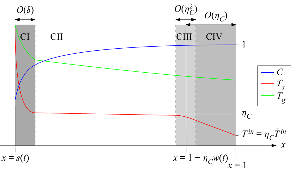
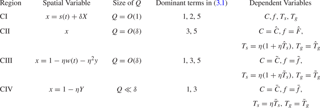
 $\mu \ll O(\log (\log (1/\delta )))$. A schematic of the asymptotic structure in this case is given in figure 6, and the changes of variable in each region is summarised in table 3.
Schematic of the solution structure in case C:  $\mu =O(1)$.

Summary of the asymptotic regions of the domain, and the changes of variable in these regions, for case C:  $\mu =O(1)$.

6.1. Region CI
As in the previous cases, we find an  $O(\delta )$ reaction region (region CI) at
 $x=s(t)$, where the heat for the reaction is provided by the radiation onto the free boundary. As before, we make the change of variables
 $x=s(t)+\delta X$, and expand the dependent variables in powers of
 $\eta _C$, by
 $$\begin{gather} T_s=T_s^{0}(X,t)+\eta_CT_s^{1}(X,t)+O\left(\eta_C^{2}\right),\quad C=C^{0}(X,t)+\eta_CC^{1}(X,t)+O\left(\eta_C^{2}\right), \end{gather}$$
 $$\begin{gather}T_g=T_g^{0}(X,t)+\eta_CT_g^{1}(X,t)+O\left(\eta_C^{2}\right), \quad f=f^{0}(X,t)+\eta_Cf^{1}(X,t)+O\left(\eta_C^{2}\right), \end{gather}$$
 $$\begin{gather}s=s_0(t)+\eta_Cs_1(t)+O\left(\eta_C^{2}\right). \end{gather}$$
We obtain the same leading-order system of (4.8a)–(4.8c) in region CI as in cases A and B. As  $X\rightarrow \infty$, we still require
 $T_s^{0}\rightarrow 0$ in order for the problem to be correctly specified. However, since the chemical reaction rate is
 $O(1)$ in the outer region, we will no longer have uniform concentration at leading order in the outer region. We must therefore impose the far-field conditions
 \begin{equation} T_s^{0}\rightarrow 0,\quad C^{0}\rightarrow C^{\infty}(t) \quad \text{ as }X\rightarrow\infty,\end{equation}
where  $C^{\infty }(t)$ is yet to be determined by matching with the outer region. Thus we can no longer solve the region CI problem independently of the rest of the domain: it is now intrinsically coupled with the outer problem, since
 $C$ varies at leading order over the outer region. The leading-order gas variables within region CI are given by (4.9), but the far-field values as
 $X\rightarrow \infty$ are now
 $$\begin{gather} f^{0}\rightarrow F_{s}(t):=f_*+(1+\dot{s}_0)(C^{\infty}-C_*), \end{gather}$$
 $$\begin{gather}T_g^{0}\rightarrow G_{s}(t):=\frac{\dfrac{f_*\rho}{s_0}+K^{{-}1}\int_{\bar{X}=0}^{\infty} T_s^{0}C^{0}\exp\left(A\left(1-\dfrac{1}{T^{0}_s}\right)\right)\,\mathrm{d}\bar{X}}{f_*+(1+\dot{s}_0)(C^{\infty}-C_*)}. \end{gather}$$
6.2. Region CII
Outside region CI, over an  $O(1)$ length scale, the heat transferred from the gas to the solid is sufficient that the chemical reaction is a dominant effect, and the solid temperature remains close to uniform. We refer to this region as region CII. Like region BII in case B, region CII is a reaction region within which the energy for the reaction is provided by the heat transferred between phases. Unlike region BII, however, the heat transfer is now fast enough that the gas temperature decreases through this region, rather than remaining uniform. In region CII, we make the rescaling
 \begin{equation} T_s=\eta_C\left(1+\eta_C\hat{T}_s\right), \end{equation}
and we also use the notation  $C=\hat {C}$,
 $f=\hat {f}$, and
 $T_g=\hat {T}_g$ for clarity. We expand the dependent variables in powers of
 $\eta _C$, setting
 \begin{equation} \left. \begin{aligned} \hat{T}_s & =\hat{T}_s^{0}(x,t)+O(\eta_C), \quad \hat{C}=\hat{C}^{0}(x,t)+O(\eta_C), \\ \hat{T}_g & =\hat{T}_g^{0}(x,t)+O(\eta_C), \quad \hat{f}=\hat{f}^{0}(x,t)+O(\eta_C). \end{aligned} \right\} \end{equation}
At leading order, the system (2.12a)–(2.12d) becomes
 $$\begin{gather} \frac{\partial{\hat{C}^{0}}}{\partial{t}}-\frac{\partial{\hat{C}^{0}}}{\partial{x}}={-}\hat{C}^{0}\exp\left(A\left(1+\hat{T}_s^{0}\right)\right), \end{gather}$$
 $$\begin{gather}\frac{\partial{\hat{f}^{0}}}{\partial{x}}=\hat{C}^{0}\exp\left(A\left(1+\hat{T}_s^{0}\right)\right), \end{gather}$$
 $$\begin{gather}\mu\hat{T}_g^{0}=\gamma\hat{C}^{0}\exp\left(A\left(1+\hat{T}_s^{0}\right)\right), \end{gather}$$
 $$\begin{gather}K\frac{\partial}{\partial x}\left(\hat{f}^{0}\hat{T}^{0}_g\right)={-}\mu\hat{T}_g^{0}. \end{gather}$$
Combining (6.7b)–(6.7d) we obtain the reduced system
 \begin{equation} \frac{\partial{\hat{f}^{0}}}{\partial{x}}=\frac{\mu}{\gamma}\hat{T}_g^{0}, \quad K\frac{\partial}{\partial x}\left(\hat{f}^{0}\hat{T}^{0}_g\right)={-}\mu\hat{T}_g^{0}, \end{equation}
for  $\hat {f}^{0}$ and
 $\hat {T}_g^{0}$. Matching with region CI, we must have
 $\hat {f}^{0}=F_{s}(t)$ and
 $\hat {T}_g^{0}=G_{s}(t)$ at
 $x=s_0$. Combining (6.8a,b), and using the boundary conditions at
 $x=s_0$, we find the first integral
 \begin{equation} \hat{f}^{0}\left(\gamma+K\hat{T}_g^{0}\right)=F_s(\gamma+KG_s).\end{equation}
Using (6.9) to eliminate  $\hat {f}^{0}$ from (6.8a), we obtain a separable equation for
 $\hat {T}_g^{0}$, namely
 \begin{equation} \frac{1}{\hat{T}_g^{0}(\gamma+K\hat{T}_g^{0})^{2}}\frac{\partial{\hat{T}_g^{0}}}{\partial{x}}={-}\frac{\mu}{\gamma KF_s(\gamma+KG_s)}, \end{equation}
with solution
 \begin{equation} \hat{T}_g^{0}(x,t)={-}\frac{\gamma W(a_{C})}{K(1+W(a_{C}))},\end{equation}
where  $W$ is the principal branch of the Lambert W function, and
 $a_{C}=a_{C}(x,t)$ is given by
 \begin{equation} a_{C}(x,t)={-}\frac{KG_{s}}{\gamma+KG_{s}}\exp\left(-\frac{1}{\gamma+KG_{s}}\left(\frac{\gamma\mu}{KF_{s}}(x-s_0)+KG_{s}\right)\right). \end{equation}
From (6.9), we therefore find
 \begin{equation} \hat{f}^{0}=\frac{F_{s}(\gamma+KG_{s})}{\gamma+K\hat{T}_g^{0}}. \end{equation}
Given  $\hat {T}_g^{0}$ from (6.11), the leading-order concentration
 $\hat {C}^{0}$ satisfies (6.7a), or
 \begin{equation} \frac{\partial{\hat{C}^{0}}}{\partial{t}}-\frac{\partial{\hat{C}^{0}}}{\partial{x}}={-}\frac{\mu}{\gamma}\hat{T}_g^{0}. \end{equation}
Matching with region CI at  $x=s_0(t)$, we require
 $\hat {C}^{0}=C^{\infty }(t)$ at
 $x=s_0(t)$, and we will see below that the correct matching condition for
 $\hat {C}^{0}$ at the right side of region CII is
 $\hat {C}^{0}=1$ at
 $x=1$. By the method of characteristics, (6.12) with the boundary condition at
 $x=1$ has solution
 \begin{equation} \hat{C}^{0}(x,t)=1-\frac{\mu}{\gamma}\int_{\xi=0}^{1-x}\hat{T}_g^{0}(1-\xi,\xi+t+x-1)\,\mathrm{d}\xi,\end{equation}
for  $\hat {T}_g^{0}(x,t)$ given by (6.11a). Evaluating at
 $x=s_0(t)$, the matching condition for
 $\hat {C}^{0}$ gives
 \begin{equation} C^{\infty}(t)=1-\frac{\mu}{\gamma}\int_{\xi=0}^{1-s_0(t)}\hat{T}_g^{0}(1-\xi,\xi+t+s_0(t)-1)\,\mathrm{d}\xi.\end{equation}
Since  $\hat {T}_g^{0}$ depends on
 $s_0$,
 $F_s$ and
 $G_s$, we see that
 $C^{\infty }$ depends on these as well. Physically, the heat and flux of gas leaving region CI determine the rate of solid material consumption in region CII, which affects the position of the free boundary
 $s_0$ (found as part of the solution of the region CI problem), and therefore the gas temperature. The processes in regions CI and CII are thus fully coupled. However, since we have solved the region CII problem to find
 $C^{\infty }(t)$, at leading order we are left with the region CI problem (4.8a)–(4.8c) with far-field condition (6.3), with
 $C^{\infty }(t)$ given by (6.14).
Concluding the analysis in region CII, we find from (6.7c) that
 \begin{equation} \hat{T}_s^{0}=\frac{1}{A}\log\left(\frac{\mu\hat{T}_g^{0}}{\gamma \hat{C}^{0}}\right)-1, \end{equation}
given the forms (6.11a) of  $\hat {T}_g^{0}$ and (6.13) of
 $\hat {C}^{0}$.
6.3. Region CIV
In region CII, we have  $T_s=\eta _C+O(\eta _C^{2})$, and so we cannot impose the boundary condition
 $T_s=T^{in}$ at
 $x=1$ (as discussed for case B, the condition (2.14) ensures
 $T^{in}<\eta _C$). There must therefore be a second boundary layer at
 $x=1$, within which the solid temperature is heated from its input temperature
 $T^{in}$ up to the critical temperature
 $\eta _C$. This heating region is analogous to region BIV in case B, and we denote it region CIV. In region CIV we change variables, setting
 \begin{equation} T_s=\eta_C\bar{T}_s, \end{equation}
with  $\bar {T}_s<1$, so that
 \begin{equation} \bar{Q}:=Q(C,\eta_C\bar{T}_s)=O\left(\delta^{1/\bar{T}_s}\right)\ll\delta, \end{equation}
and thus we cannot expect a dominant balance in the solid heat equation (2.12c) between the heating from the gas and heat lost to chemical reaction. Instead, we find a balance between the heating from the gas and the advection term, which fixes the length scale of region CIV to be  $O(\eta _C)$. Within region CIV we therefore make the change of variables
 $x=1-\eta _C Y$, where
 $Y=O(1)$ is positive. For clarity of notation, we set
 $C=\bar {C}$,
 $f=\bar {f}$ and
 $T_g=\bar {T}_g$ in region CIV, and we also rewrite the input temperature
 $T^{in}=\eta _C\bar {T}^{in}$, so that the boundary condition becomes
 \begin{equation} \bar{T}_s=\bar{T}^{in} \quad \text{ at }Y=0. \end{equation}
Again, we expand in powers of  $\eta _C$, setting
 \begin{equation} \left. \begin{aligned} \bar{T}_s & =\bar{T}_s^{0}(Y,t)+O(\eta_C), \quad \bar{C}=\bar{C}^{0}(Y,t)+O(\eta_C), \\ \bar{T}_g & =\bar{T}_g^{0}(Y,t)+O(\eta_C), \quad \bar{f}=\bar{f}^{0}(Y,t)+O(\eta_C). \end{aligned} \right\} \end{equation}
Due to the short length scale, at leading order in (2.12a), (2.12b) and (2.12d), we see that all of  $\bar {C}^{0}$,
 $\bar {f}^{0}$ and
 $\bar {T}_g^{0}$ are uniform across region CIV. The boundary condition at
 $Y=0$ (or
 $x=1$) fixes
 $\bar {C}^{0}=1$, while
 $\bar {f}^{0}$ and
 $\bar {T}_g^{0}$ must be fixed by matching to the left. At leading order in (2.12c), we find that the solid temperature
 $\bar {T}_s^{0}$ satisfies
 \begin{equation} \frac{\partial{\bar{T}_s^{0}}}{\partial{Y}}=\mu\bar{T}_g^{0}, \end{equation}
and thus, using the boundary condition (6.18), we find that  $\bar {T}_s^{0}$ is linear in
 $Y$
 \begin{equation} \bar{T}_s^{0}=\bar{T}^{in}+\mu\bar{T}_g^{0}Y. \end{equation}
6.4. Region CIII
Exactly as in case B, the solution (6.21) in region CIV is valid only while  $\bar {T}_s^{0}<1$, and we cannot directly match the linear profile (6.21) with the constant
 $T_s\sim \eta _C$ in region CII. Thus, as in case B, we must introduce a transition layer, region CIII, between regions CII and CIV, in which the heat transferred from the gas is no longer used in the chemical reaction, but is instead used to heat the solid material from its input temperature
 $T^{in}$. In this transition layer, we must have
 $T_s\approx \eta _C$, and we expect a balance between all three of heat advection (term 1), heat transfer from the gas (term 3) and heat loss to the chemical reaction (term 5) in (3.1). The length scale of such a region must therefore be
 $O(\eta _C^{2})$. We may show, as in case B, that all of
 $f$,
 $T_g$ and
 $C$ are uniform across region CIII, so that matching across CII–CIV, we find
 \begin{equation} \hat{C}^{0}|_{x=1} =\bar{C}^{0}=1, \quad F_1(t):=\hat{f}^{0}|_{x=1} =\bar{f}^{0}, \quad G_1(t):=\hat{T}_g^{0}|_{x=1} =\bar{T}_g^{0}. \end{equation}
(This fixes the boundary condition at  $x=1$ for
 $\hat {C}^{0}$, in region CII.) As in case B, we find that the ODE for the solid temperature variation simply smooths the transition from region CII to region CIV. The changes of variable for this analysis are summarised in table 3. The position
 $w(t)$ of the transition layer is found by matching
 $T_s$ across regions CIII–CIV, which, at leading order, requires
 $1=\bar {T}^{in}+\mu G_1 w,$ so that
 \begin{equation} w(t)=\frac{1}{\mu G_1(t)}\left(1-\bar{T}^{in}\right).\end{equation}
6.5. Composite solution
As in previous cases, we may construct a leading-order composite solution. Since  $C$,
 $f$ and
 $T_g$ are
 $O(1)$ in all regions, and uniform in regions CIII and CIV, the composite solutions are
 $$\begin{gather} C^{C}=C^{0}\left(\frac{x-s_0(t)}{\delta}\right)+\hat{C}^{0}(x,t)-C^{\infty}(t), \end{gather}$$
 $$\begin{gather}f^{C}=f^{0}\left(\frac{x-s_0(t)}{\delta}\right)+\hat{f}^{0}(x,t)-F_s(t), \end{gather}$$
 $$\begin{gather}T_g^{C}=T_g^{0}\left(\frac{x-s_0(t)}{\delta}\right)+\hat{T}_g^{0}(x,t)-G_s(t). \end{gather}$$
The solid temperature is  $O(1)$ in region CI but
 $O(\eta _C)$ elsewhere. We therefore construct a composite solution by setting the
 $O(\eta _C)$ correction in region CI to be simply
 $\eta _C$, so that the composite solution is accurate at leading order in all regions. As in case B, the composite solution for
 $T_s$ is defined piecewise about the centre,
 $1-\eta _Cw(t)$, of the transition layer CIII. Thus we use the composite solution
 \begin{equation} T_s^{C}=\begin{cases} T_s^{0}\left(\dfrac{x-s_0(t)}{\delta}\right)+\eta_C, & \text{if }x<1-\eta_C w(t),\\ \eta_C\bar{T}_s^{0}\left(\dfrac{1-x}{\eta_C}\right), & \text{if }x\geq 1-\eta_C w(t). \end{cases} \end{equation}
We have seen that case C is very similar to case B. In each, the solid is heated up from its input temperature  $T^{in}$ by heat transferred from the gas in region IV. Once it has reached the critical temperature
 $\eta$ the chemical reaction then starts to take place, and the heat transferred from the gas to the solid in this region (II) is used primarily for this reaction, with no change in the solid temperature at leading order until it reaches the hot boundary layer (I) at
 $x=s$. The differences in case C are that, since the convective heat transfer from the gas is now greater, the solid material heats up much faster (over the
 $O(\eta _C)$ length scale of region CIV, rather than the
 $O(1)$ length scale of BIV), and that the reaction rate in region CII is now high enough to affect all of the solid concentration
 $C$, gas mass flux
 $f$ and gas temperature
 $T_g$ at leading order. As we increase
 $\mu$ still further, the gas temperature must lose so much heat to the solid that it ceases to be
 $O(1)$. This is the situation considered in case D below.
7. Case D: $-\log (\eta )\ll \mu \ll \delta ^{-1}e^{-A}$, large heat transfer

We notice that the analysis in case C above, with  $\mu =O(1)$, holds so long as
 $T_g$ remains
 $O(1)$ over the entirety of the domain. From the form (6.11) of
 $\hat {T}_g$ in region CII, we see that for large enough values of the convective heat-transfer coefficient
 $\mu$,
 $\hat {T}_g$ will decay quickly enough to become
 $O(\eta )$ within the domain, at which point the equations (6.7) of region II are no longer valid.
In this section we study the case  $\mu \gg 1$, for which
 $T_g$ becomes
 $O(\eta )$ within the domain. Since
 $\mu \gg 1$, the heat transfer between phases is fast enough that the two temperatures
 $T_s$ and
 $T_g$ become near equal over a short length scale. We find that the length scale over which the temperatures equilibrate in this way is
 $O(-\log (\eta )/\mu )$. In this section, we therefore restrict our attention to the case where the convective heat-transfer coefficient
 $\mu$ is sufficiently large,
 $\mu \gg -\log (\eta )\gg 1$, that the two temperatures equilibrate over a length scale smaller than
 $O(1)$, i.e. within the domain
 $x\in [s,1]$. With
 $\mu \gg 1$, the solid temperature scaling (3.2), is denoted
 $\eta _D$, and we note
 $\eta _D>\eta _C>\eta _B$. We also require that
 $\mu \ll \delta ^{-1} e^{-A}$, so that
 $\eta _D\ll 1$. This ensures that the asymptotic expansion in powers of
 $\eta _D$ remains valid. Although not strictly a distinguished limit of the problem, it is interesting to study this regime
 $-\log (\eta _D)\ll \mu \ll \delta ^{-1} e^{-A}$ in order to understand how the solution structure evolves as
 $\mu$ increases from
 $O(1)$ in case C to the distinguished limit
 $\mu =O(\delta ^{-1})$, which we study in case E below. Specifically, all of the chemical reaction in case D occurs in a (wide,
 $O(-\log (\eta )/\mu )$) boundary layer about the free boundary
 $x=s$, whereas in case C the chemical reaction occurred throughout the entire
 $O(1)$ domain (except in a heating boundary layer located at
 $x=1$). This is because the heat transfer between phases now occurs much faster. (In case E, with the inter-phase heat transfer faster still, we will see that the reaction regions are confined to an even narrower region around
 $x=s$.)
We will not study the case  $1\ll \mu \ll -\log (\eta _D)$, since this limit has the same structure of case C, as we will show below. We also do not deal fully with the distinguished limit
 $\mu =O(-\log (\eta _D))$, since there is a plethora of subcases for the asymptotic structure in this case, depending on whether the two temperatures equilibrate over the domain or not, and how close the point at which they equilibrate is to the boundary
 $x=1$ of the domain. We discuss some of these possible subcases in more detail in the discussion below.
Although in cases C (above) and E (below) we find time-dependent solutions, in case D we restrict our attention to the steady-state case, for simplicity. We note, however, that time-dependent solutions in case D are likely to have the same structure as those we later discuss in cases E and F, below. We find that there are two separate steady-state behaviours in the regime  $-\log (\eta _D)\ll \mu \ll \delta ^{-1}e^{-A}$, depending on the model parameters. Specifically, in case Da we suppose
 $Kf<1$ near
 $x=1$, so that the heat flux in the gas is smaller in magnitude than the heat flux in the solid in the opposite direction. In case Db we consider the opposite case, in which
 $Kf>1$ near
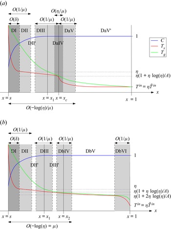
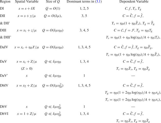
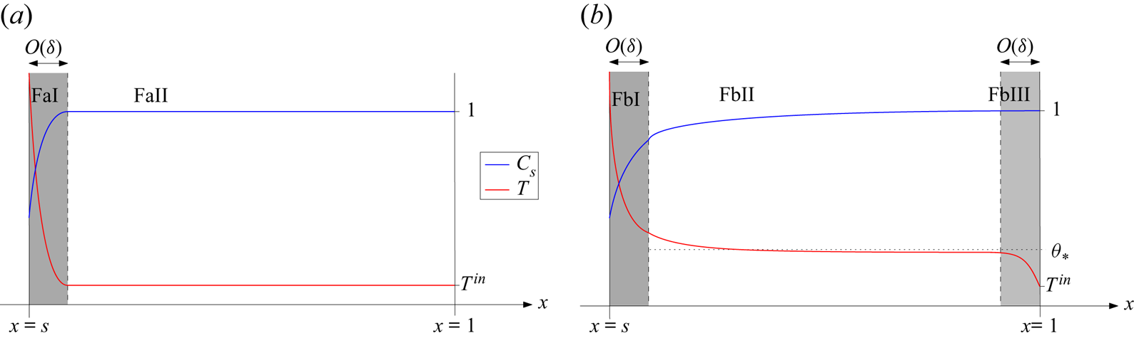
 $x=1$. The schematics illustrating the solution structure in these two steady-state cases Da and Db are shown in figure 7, and the changes of variable for each region are summarised in table 4.
Schematics of the steady-state solution structures in case D:  $\mu =O(1)$. (a) Case Da,
 $KF_*<1$. (b) Case Db,
 $KF_*>1$.

Summary of the asymptotic regions of the domain, and the changes of variable in these regions, for the steady-state cases D (a and b):  $-\log (\eta _D)\ll \mu \ll \delta ^{-1}$.

7.1. Behaviour common to cases Da and Db
There are several regions of the domain near to the free boundary  $x=s$ where the behaviour is the same for both cases Da and Db.
7.1.1. Region DI
As usual we find a reaction boundary layer, region DI, of width  $O(\delta )$ at
 $x=s$, within which the heat for the reaction is provided by the radiation onto the free boundary. Expanding the dependent variables in powers of
 $\eta _D$, by setting
 $$\begin{gather} T_s=T_s^{0}(X)+\eta_DT_s^{1}(X)+O\left(\eta_D^{2}\right), \quad C=C^{0}(X)+\eta_DC^{1}(X)+O\left(\eta_D^{2}\right), \end{gather}$$
 $$\begin{gather}T_g=T_g^{0}(X)+\eta_DT_g^{1}(X)+O\left(\eta_D^{2}\right), \quad f=f^{0}(X)+\eta_Df^{1}(X)+O\left(\eta_D^{2}\right), \end{gather}$$
 $$\begin{gather}s=s_0+\eta_Ds_1+O\left(\eta_D^{2}\right), \end{gather}$$
we obtain the same equations (4.8a)–(4.8c) at leading order since  $\mu \ll \delta ^{-1}$ (although with
 $\dot {s}_0=0$, since we restrict ourselves to steady-state solutions). The far-field solid concentration must satisfy (6.3) as in case C, where
 $C^{\infty }$ is yet to be determined by matching with the outer problem.
7.1.2. Region DII
Outside region DI, we require  $T_s\sim \eta _D$, in order to balance the terms 3 and 5 in the solid heat equation (3.1). However, since then
 $Q=O(\mu )\gg 1$, this region, which we denote region DII, must have a shorter length scale than
 $O(1)$ in order to obtain a balance in the gas temperature equation. In this region the heat for the reaction is provided by the heat transfer between phases. Region DII is therefore a second, wider boundary layer, width
 $O(\mu ^{-1})$, about
 $x=s_0$, and so we make the change of variables
 $x=s_0+y/\mu$. We look for a solution
 \begin{equation} T_s=\eta_D\left(1+\eta_D\hat{T}_s\right), \end{equation}
and we also use the notation  $C=\hat {C}$,
 $f=\hat {f}$, and
 $T_g=\hat {T}_g$ in region DII for clarity. We expand in powers of
 $\eta _D\ll 1$, setting
 \begin{equation} \left. \begin{aligned} \hat{T}_s & =\hat{T}_s^{0}(y)+O(\eta_D), \quad \hat{C}=\hat{C}^{0}(y)+O(\eta_D),\\ \hat{T}_g & =\hat{T}_g^{0}(y)+O(\eta_D), \quad \hat{f}=\hat{f}^{0}(y)+O(\eta_D). \end{aligned} \right\} \end{equation}
Substituting into (2.12a)–(2.12d), we find that at leading order
 $$\begin{gather} -\frac{\mathrm{d}{\hat{C}^{0}}}{\mathrm{d}{y}}={-}\hat{C}^{0}\exp\left(A\left(1+\hat{T}_s^{0}\right)\right), \quad \hat{T}_g^{0}=\gamma\hat{C}^{0}\exp\left(A\left(1+\hat{T}_s^{0}\right)\right), \end{gather}$$
 $$\begin{gather}\frac{\mathrm{d}{\hat{f}^{0}}}{\mathrm{d}{y}}=\hat{C}^{0}\exp\left(A\left(1+\hat{T}_s^{0}\right)\right), \quad K\frac{\mathrm{d}}{\mathrm{d} y}(\hat{f}^{0}\hat{T}_g^{0})={-}\hat{T}_g^{0}. \end{gather}$$
Precisely as in (6.11) for region CII of case C, we find the solutions
 \begin{equation} \hat{T}_g^{0}={-}\frac{\gamma W(a_{D})}{K(1+W(a_{D}))}, \quad \hat{f}^{0}=\frac{F_s(\gamma+KG_s)}{\gamma +K\hat{T}_g^{0}}, \end{equation}
of (7.4b), where
 \begin{equation} a_{D}={-}\frac{KG_s}{\gamma+KG_s}\exp\left(-\frac{1}{\gamma+KG_s}\left(\frac{\gamma }{KF_s}y+KG_s\right)\right), \end{equation}
and the matching constants  $F_s$ and
 $G_s$ are as defined in (6.4) (with
 $\dot {s}_0=0$, since we are in steady state). The leading-order solid concentration therefore satisfies
 \begin{equation} -\frac{\mathrm{d}{\hat{C}^{0}}}{\mathrm{d}{y}}=\frac{W(a_{D})}{K(1+W(a_{D}))},\end{equation}
along with  $\hat {C}^{0}=C^{\infty }$ at
 $y=0$, and a matching condition to the right, as
 $y$ becomes large. We will find below that
 $C$ is uniform to leading order in all regions to the right of region DII, in both cases Da and Db. Thus the matching condition is
 $\hat {C}^{0}\rightarrow 1$ as
 $y\rightarrow \infty.$ From (7.5a) we see that
 $\hat {T}_g^{0}\rightarrow 0$ as
 $y\rightarrow \infty$, and so the solution of (7.7) is
 \begin{equation} \hat{C}^{0}=1-\frac{KF_s(\gamma+KG_s)\hat{T}_g^{0}}{\gamma(\gamma+K\hat{T}_g^{0})}. \end{equation}
Applying the boundary conditions at  $y=0$, where
 $\hat {T}_g^{0}=G_s$, we therefore fix the value of
 $C^{\infty }$ to be
 \begin{equation} C^{\infty}=1-\frac{KF_sG_s}{\gamma}. \end{equation}
Having found  $\hat {T}_g^{0}$ and
 $\hat {C}^{0}$, the solid temperature variation, given by (7.4a) (right), is then
 \begin{align} \hat{T}_s^{0}&=\frac{1}{A}\log\left(\frac{\hat{T}_g^{0}}{\gamma \hat{C}^{0}}\right)-1\nonumber\\ &={-}1-\frac{1}{A}\log\left(K\left(1+W(a_{D})\right)\left(\frac{1}{-W(a_{D})}-\frac{F_s(\gamma+KG_s)}{\gamma}\right)\right). \end{align}
We note that this region DII is exactly analogous to region CII in case C with  $\mu =O(1)$, except that, since the convective heat-transfer coefficient
 $\mu$ is now larger, the decay length of
 $\hat {T}_g^{0}$ is shorter. We see that (7.4) hold until
 $\hat {T}_g^{0}$ becomes order
 $\eta _D$, at which point term 4 must enter the dominant balance of (3.1). Since for small
 $a_{D}$,
 $W(a_{D})\sim a_{D}$, we see that
 $\hat {T}_g^{0}\sim \eta _D$ when
 $-\gamma a_{D}/K=\eta _D$, which occurs at the point
 $y=y_*$, defined by
 $\gamma a_{D}(y_*)/K=\eta _D$. Rearranging, this gives
 \begin{equation} y_*=\frac{1}{\gamma}KF_s(\gamma+KG_s)\left(-\log(\eta_D)+\log\left(\frac{\gamma G_s}{\gamma +KG_s}\right)-\frac{KG_s}{\gamma+KG_s}\right).\end{equation}
We see that point  $y_*=O(-\log (\eta _D))$ is large. As
 $y$ becomes larger than
 $O(1)$, we strictly leave region DII, and enter region DII’, an extension of DII, within which the length scale is
 $O(-\log (\eta _D)/\mu )$. The dominant physical processes in region DII’ (heat transfer from gas to solid, which provides energy for the chemical reaction) are the same as in region DII, except that
 $f$ is uniform at leading order, and thus
 $T_g$ is exponentially decaying.
In the original variables, the point  $y_*$ is at
 $x_1:=s_0+y_*/\mu$. As mentioned at the start of this section, we notice that if
 $1\ll \mu \ll -\log (\eta _D)$ then
 $x_1-s_0\gg 1$ and so we revert to a structure like case C, since
 $\hat {T}_g$ remains
 $O(1)$ throughout the domain. Conversely, in the regime
 $-\log (\eta _D)\ll \mu$ studied in this section, we have
 $x_1-s_0\ll 1$ and so
 $\hat {T}_g^{0}$ becomes small within the domain. In the distinguished limit
 $\mu =O(-\log (\eta _D))$, we see that
 $x_1-s_0=O(1)$, and we may be in either of these cases, or instead have
 $x_1$ close to
 $1$, for which a number of additional subcases arise.
7.1.3. Region DIII
With  $\mu \gg -\log (\eta _D)$, the point
 $x_1$ is an
 $O(-\log (\eta _D)/\mu )\ll 1$ distance from
 $s_0$ (and so is definitely contained within the domain). Around this point
 $x_1$, there must be an
 $O(\mu ^{-1})$ transition layer, denoted region DIII, in which term 4 enters the dominant balance in (3.1). In this region we use the change of spatial variables
 $x=x_1+z/\mu$. Since now
 $T_g=O(\eta _D)$, the balance of terms 3 and 5 requires that term 5, the chemical reaction rate, be
 $O(\delta \mu \eta _D)$. Heat transfer between the two phases is slower than in regions DII-DII’ since the difference between the two temperatures is now smaller, and so the chemical reaction driven by this temperature difference is slower in this region than in region DII and DII’. Thus, the solid temperature must be of the form
 \begin{equation} T_s=\eta_D\left(1+\frac{\eta_D\log(\eta_D)}{A}+\eta_D\mathcal{T}_s\right).\end{equation}
We also use the change of variables  $T_g=\eta _D\mathcal {T}_g$ in region DIII, and set
 $f=\mathcal {F}$,
 $C=\mathcal {C}$ for clarity of notation, and we expand in powers of
 $\eta _D$, setting
 \begin{equation} \left. \begin{aligned} \mathcal{T}_s & =\mathcal{T}_s^{0}(z)+O(\eta_D), \quad \mathcal{C}=\mathcal{C}^{0}(z)+O(\eta_D), \\ \mathcal{T}_g & =\mathcal{T}_g^{0}(z)+O(\eta_D), \quad \mathcal{F}=\mathcal{F}^{0}(z)+O(\eta_D). \end{aligned} \right\} \end{equation}
At leading order in (2.12a) and (2.12b), we find that both  $\mathcal {C}^{0}$ and
 $\mathcal {F}^{0}$ are uniform in region DIII. This is because the chemical reaction rate is now
 $Q=O(\delta \eta _D\mu )$, and so there is only an
 $O(\eta _D)$ mass consumption over region DIII. Indeed, we will find that in all regions to the right of region DIII (in either case Da or Db),
 $C$ and
 $f$ are uniform up to
 $O(\eta _D)$. Thus by matching to the right we will find that
 $\mathcal {C}^{0}=1$, and matching at leading order with region DII, we have
 \begin{equation} \mathcal{F}^{0}=F_*:=\frac{F_s(\gamma+KG_s)}{\gamma}=\hat{f}^{0}|_{y=y_*}+O(\eta_D). \end{equation}
At leading order, the heat equations (2.12c) and (2.12d) for  $\mathcal {T}_s^{0}$ and
 $\mathcal {T}_g^{0}$ become
 $$\begin{gather} \mathcal{T}_g^{0}-\left(1+\eta_D\frac{\log(\eta_D)}{A}\right)=\gamma \exp\left(A\left(1+\mathcal{T}_s^{0}\right)\right), \end{gather}$$
 $$\begin{gather}KF_*\frac{\mathrm{d}{\mathcal{T}_g^{0}}}{\mathrm{d}{z}}={-}\mathcal{T}_g^{0}+\left(1+\eta_D\frac{\log(\eta_D)}{A}\right). \end{gather}$$
Here, we have included the  $O(-\eta _D\log (\eta _D))$ terms, since these are larger than the next order
 $\eta _D$, and we can find an explicit solution taking both
 $O(1)$ and
 $O(-\eta _D\log (\eta _D))$ terms into account together. The ODE (7.16) for
 $\mathcal {T}_g^{0}$ has the general solution
 \begin{equation} \mathcal{T}_g^{0}=1+\eta_D\frac{\log(\eta_D)}{A}+\exp\left(-\frac{1}{KF_*}z\right), \end{equation}
where we have fixed the constant of integration by matching with region DII. Finally, from (7.15) we compute
 \begin{equation} \mathcal{T}_s^{0}={-}\frac{1}{A}\left(\log(\gamma)+\frac{1}{KF_*}z\right)-1, \end{equation}
completing the analysis in region DIII.
7.1.4. Regions DaV and DbVI
Regions DI–DIII as described above are common to both cases Da and Db; these are all reaction regions, with the chemical reaction playing a dominant role. We now pause in our analysis moving left to right through the domain, and instead investigate the behaviour near the  $x=1$ boundary, where there is negligible chemical reaction. We will find different behaviour for the cases Da and Db, depending on whether the overall heat flux
 $Kf-1=KF_*-1+O(\eta _D)$ is negative or positive, respectively.
On the right side of the domain, the solid temperature must decrease from close to  $\eta _D$ at the left of the domain to the input value
 $T^{in}=\eta _D\bar {T}^{in}$. (As in regions BIV and CIV, here the heat transferred from the gas to the solid is used to heat the solid material from its input temperature,
 $T^{in}$). We therefore rescale
 \begin{equation} T_s=\eta_D\bar{T}_s \quad \text{and} \quad T_g=\eta_D\bar{T}_g, \end{equation}
noting that  $T_g$ must be
 $O(\eta _D)$ in this region too because it is
 $O(\eta _D)$ in region DIII, and can only decrease through the rest of the domain. With
 $\bar {T}_s<1+\eta _D\log (\eta _D)/A$, we notice that the chemical reaction rate
 $\bar {Q}\ll \delta \mu \eta _D$ is small. In order to balance the heat advection with heat transfer between phases in the gas heat equation, we must scale the space variable to an
 $O(1/\mu )$ domain. Thus the region over which
 $T_s$ changes must be a boundary layer. We make the change of variables
 $x=x_c+Z/\mu$, where
 $Z=O(1)$, and
 $x_c$ (the position of this boundary layer) is an
 $O(1)$ point in the domain, to be determined. As well as (7.19a,b), we set
 $f=\bar {f}$ and
 $C=\bar {C}$ in this region for clarity of notation, but note that since
 $\bar {Q}\ll \delta \mu \eta _D$ is small,
 $\bar {C}=1+O(\eta _D)$ and
 $\bar {f}^{0}=F_*+O(\eta _D)$ are uniform over this region at leading order, fixed by matching with regions to the right and left, respectively. We expand the temperatures in powers of
 $\eta _D$, by setting
 \begin{equation} \bar{T}_s=\bar{T}_s^{0}(Z)+O(\eta_D), \quad \bar{T}_g=\bar{T}_g^{0}(Z)+O(\eta_D). \end{equation}
At leading order in (2.12c) and (2.12d), we therefore find
 \begin{equation} -\frac{\mathrm{d}{\bar{T}_s^{0}}}{\mathrm{d}{Z}}=\bar{T}_g^{0}-\bar{T}_s^{0}, \quad KF_*\frac{\mathrm{d}{\bar{T}_g^{0}}}{\mathrm{d}{Z}}={-}\bar{T}_g^{0}+\bar{T}_s^{0}, \end{equation}
which admit a general solution
 \begin{equation} \bar{T}_s^{0}=b_1+KF_*b_2\exp\left(\frac{KF_*-1}{KF_*} Z\right), \quad \bar{T}_g^{0}=b_1+b_2\exp\left(\frac{KF_*-1}{KF_*}Z\right), \end{equation}
where  $b_1$ and
 $b_2$ are constants to be determined. We notice that the position of the boundary layer,
 $x_c$, must depend on the sign of
 $KF_*-1$, and we consider the cases Da (
 $KF_*<1$) and Db (
 $KF_*>1$) separately below. In case Da with
 $KF_*<1$, we find that this boundary layer must be at the left side of the domain (region DaV), whereas in case Db with
 $KF_*>1$, we must take
 $x_c=1$ so that the boundary layer is region DbVI, on the right side of the domain. From the non-dimensionalisation, we see that
 \begin{equation} KF_*<1 \quad \text{if}\quad c_{p,g}f< c_{p,s}u_sC_s, \end{equation}
and vice versa. Thus, since both phases have the same temperature at leading order on an  $O(1)$ length scale, we are comparing the heat flux in the gas (left-to-right) with that in the solid (right-to-left).
7.2. Case Da: $KF_*<1$

If  $KF_*<1$, then the heat flux in the solid is greater than that in the gas, and so the overall heat transport is right-to-left.
7.2.1. Region DaV
From the form of the solution (7.22a,b), we require that  $x_c$ is on the left side of the domain, so that the solution remains bounded as
 $Z\rightarrow \infty$ and we leave the boundary layer. This boundary layer is denoted region DaV in figure 7.
As  $Z\rightarrow \infty$, we have
 $\bar {T}_s^{0},\bar {T}_g^{0}\rightarrow b_1$, so in this case we must take
 $b_1=\bar {T}^{in},$ in order to satisfy the boundary condition at
 $x=1$. The value of
 $b_2$ is fixed by matching at
 $Z=0$, or
 $x=x_c$. We notice that the difference in solutions at
 $Z=0$ is
 \begin{equation} (\bar{T}_g^{0}-\bar{T}_s^{0})\Big|_{Z=0}=(1-KF_*)b_2=O(1), \end{equation}
thus  $T_g-T_s=O(\eta _D)$ at
 $Z=0$. We must therefore have
 $x_c$ within the
 $O(1/\mu )$ transition layer DIII about
 $x_1$, in which
 $T_g-T_s=O(\eta _D)$. Since
 $T_s=\eta _D(1+\eta _D\log (\eta _D)/A)+O(\eta _D^{2})$ (by (7.12)) throughout region DIII, we fix
 $b_2$ to be
 \begin{equation} b_2=\frac{1}{KF_*}\left(1+\eta_D\frac{\log(\eta_D)}{A}-\bar{T}^{in}\right). \end{equation}
Thus the solutions (7.22a,b) in this boundary-layer region DaV (to the right of  $x=x_c$) are
 $$\begin{gather} \bar{T}_s^{0}=\bar{T}^{in}+\left(1+\eta_D\frac{\log(\eta_D)}{A} -\bar{T}^{in}\right)\exp\left(-\frac{1-KF_*}{KF_*} Z\right), \end{gather}$$
 $$\begin{gather}\bar{T}_g^{0}=\bar{T}^{in}+\frac{1}{KF_*}\left(1+\eta_D\frac{\log(\eta_D)}{A} -\bar{T}^{in}\right)\exp\left(-\frac{1-KF_*}{KF_*} Z\right). \end{gather}$$
At  $x=x_c$, or
 $Z=0$, we have
 $\bar {T}_g^{0}=(1+\eta _D\log (\eta _D)/A)/(KF_*)$. Imposing continuity of
 $T_g$ at
 $x=x_c$ determines the position of
 $x_c$ within region DIII, i.e.
 $x_c$ is the point at which
 \begin{equation} \mathcal{T}_g^{0}=\frac{1+\eta_D\log(\eta_D)/A}{KF_*}. \end{equation}
Using the form of  $\mathcal {T}_g^{0}$ given by (7.17), we find that
 \begin{equation} x_c=x_1+\frac{1}{\mu}KF_*\log\left(\frac{1}{(1-KF_*)(1+\eta_D\log(\eta_D)/A)}\right).\end{equation}
7.2.2. Region DaIV
In order to match between the  $O(1/\mu )$ regions DIII and DaV on either side of
 $x_c$, we must introduce a narrower transition layer of width
 $O(\eta _D/\mu )$ at
 $x=x_c$, which we refer to as region DaIV. This region is entirely analogous to regions BIII and CIII, in that its only function is to smooth the transition between neighbouring regions. Exactly as in those cases we see that all of
 $f$,
 $C$ and
 $T_g$ are uniform to leading order over this region (although, unlike cases B and C,
 $T_g$ is now
 $O(\eta _D)$), and we are left with a single ODE for the solid temperature variation. The changes of variable for this analysis are given in table 4.
To the right of region DaV is region DaV’, filling the remainder of the domain. This is an extension of region DaV, in which all variables are uniform at leading order, with  $C=1+O(\eta _D)$,
 $f=F_*+O(\eta _D)$,
 $T_s=\eta _D\bar {T}^{in}+O(\eta _D^{2})$ and
 $T_g=T_s+O(\eta _D^{2})$.
7.2.3. Composite solution
We can form a leading-order, composite, steady-state solution as follows. Since  $C=1$ at leading order in regions DIII-DaV’, the leading-order composite solution is simply
 \begin{equation} C^{Da}=C^{0}\left(\frac{x-s_0}{\delta}\right)+\hat{C}^{0}(\mu(x-s_0))-C^{\infty}. \end{equation}
The gas temperature is  $O(1)$ in regions DI and DII, but
 $O(\eta _D)$ in regions DIII–DaV’. Since we have not computed the
 $O(\eta _D)$ correction in regions DI–DII, we assume that this correction is
 $\eta _D(1+\eta _D\log (\eta _D)/A)$ so that the composite solution is correct to
 $O(\eta _D)$ in regions DIII–DaV’. The composite solution is defined piecewise on either side of the transition layer DaIV. The centre of this transition layer is
 $x_c$, given by (7.28), which is defined so that there is a continuous transition between
 $T_s=\eta _D\mathcal {T}_g^{0}$ in region DIII and
 $T_s=\eta _D\bar {T}_g$ in region DaV. For the composite solution, we choose to define a slightly different changeover point
 $x_c^{*}=x_c+O(\eta _D/\mu )$, so that the composite solution is continuous at this point. We therefore use
 \begin{equation} T_g^{Da}=\begin{cases} T_g^{0}\left(\dfrac{x-s_0}{\delta}\right)+\hat{T}_g^{0}(\mu(x-s_0))-G_s & \\ \quad +\eta_D\mathcal{T}_g^{0}(\mu(x-x_1))-\exp\left(-\dfrac{\mu}{KF_*}(x-x_1)\right), & \text{if }x< x_c^{*},\\ \eta_D\bar{T}_g^{0}(\mu(x-x_c)), & \text{if }x>x_c^{*}, \end{cases} \end{equation}
which, from the form of  $\mathcal {T}_g^{0}$ in (7.17), simplifies to
 \begin{equation} T_g^{Da}=\begin{cases} T_g^{0}\left(\dfrac{x-s_0}{\delta}\right)+\hat{T}_g^{0}(\mu(x-s_0))-G_s+\eta_D\left(1+\eta_D\dfrac{\log(\eta_D)}{A}\right), & \text{if }x< x_c^{*},\\ \eta_D\bar{T}_g^{0}(\mu(x-x_c)), & \text{if }x>x_c^{*}. \end{cases} \end{equation}
The solid temperature is similarly  $O(1)$ in region DI, but
 $O(\eta _D)$ everywhere else. As in previous cases, we set the
 $O(\eta _D)$ correction in region DI to be
 $\eta _D(1+\eta _D\log (\eta _D)/A)$ so that the composite solution is accurate to
 $O(\eta _D)$ in regions DII–DaV’. We neglect the
 $O(\eta _D^{2})$ corrections in regions DII and DIII for this composite solution. We form the leading-order composite solution
 \begin{equation} T_s^{Da}= \begin{cases} T_s^{0}\left(\dfrac{x-s_0}{\delta}\right)+\eta_D\left(1+\eta_D\dfrac{\log(\eta_D)}{A}\right), & \text{if }x< x_c,\\ \eta_D\bar{T}_s^{0}(\mu(x-x_c)), & \text{if }x>x_c. \end{cases} \end{equation}
7.3. Case Db: $KF_*>1$

In the case  $KF_*>1$, the heat flux in the gas is greater than in the solid. We therefore require the position of the boundary layer over which
 $T_s$ decays to
 $T_s^{in}$ to be at the far right of the domain, at
 $x_c=1$. This is so that the variable
 $Z<0$, and the solution (7.22a,b) is bounded as we leave the boundary layer (
 $Z\rightarrow -\infty$). This boundary layer is therefore region DbVI in figure 7.
In this case, we notice that as  $Z\rightarrow -\infty$, both
 $\bar {T}_s^{0},\bar {T}_g^{0}\rightarrow b_1$, so that far from
 $x=1$, we have
 $T_g-T_s=O(\eta _D^{2})$. In region DIII, we have
 $T_g-T_s=O(\eta _D)$. We therefore cannot match directly with region DIII: there must be another region within which
 $T_s-T_g=O(\eta _D^{2})$. We denote this region DbIV.
7.3.1. Region DbIV
We note that the analysis of region DIII holds so long as  $T_g-T_s\gg \eta _D^{2}$. As
 $T_g$ is decaying through region DIII,
 $T_g-T_s$ is decreasing. At the point where
 $T_g-T_s=O(\eta _D^{2})$, the advection (term 1 in (3.1)) must also enter be included in the dominant balance. From (7.17), we see that
 $T_g-T_s=\eta _D^{2}$ when
 \begin{equation} \exp\left(-\frac{1}{KF_*}z\right)=\eta_D, \end{equation}
i.e. at the point
 \begin{equation} z_*={-}KF_*\log(\eta_D). \end{equation}
Like  $y_*$ given by (7.11), we note that
 $z_*=O(-\log (\eta _D))$ is large. Strictly speaking, there is therefore another region DbIII’ with length scale
 $O(-\log (\eta _D)/\mu )$ to the right of region DIII, but since this is a subregion of region DIII (the same equations hold, simply over a longer length scale), we do not analyse this region separately. Although
 $z_*$ is large, in the original variables, this is the point
 $x_2:=s_0+(y_*+z_*)/\mu \ll 1$, since
 $\mu \gg -\log (\eta _D)$. Thus
 $x_2$ remains within the
 $O(-\log (\eta _D)/\mu )$ boundary layer around
 $x=s_0$.
Region DbIV is the transition layer around the point  $x_2$, in which all the terms 1, 3, 4 and 5 balance in the solid heat equation (3.1). Since
 $T_g-T_s=O(\eta _D^{2})$ in region DbIV, we make the change of variables
 \begin{align} T_s=\eta_D\left(1+2\eta_D\frac{\log(\eta_D)}{A}+\eta_D\frac{\tau_s}{A}\right), \quad T_g=\eta_D\left(1+2\eta_D\frac{\log(\eta_D)}{A}+\eta_D\frac{\tau_g}{A}\right), \end{align}
so that at leading order both  $T_s$ and
 $T_g$ are uniform through region DbIV. The heat exchange terms (3 and 4) now combine to be
 $O(\mu \eta _D^{2})$, and the heat lost to the chemical reaction (term 5) is likewise
 $O(\mu \eta _D^{2})$, since
 \begin{equation} Q(C,T_s)=\delta \mu\left(\eta_D^{2}Ce^{A+\tau_s}+O\left(\eta_D^{3}\right)\right). \end{equation}
As in regions DII and DIII, we require an  $O(1/\mu )$ length scale to balance advection and heat transfer terms in the gas heat equation, and so we make the change of variables
 $x=x_2+Z/\mu$. As in region DIII, we note that since the reaction rate is small,
 $C=1+O(\eta _D)$,
 $f=F_*+O(\eta _D)$ are uniform at leading order throughout this region. Expanding in powers of
 $\eta _D$, taking
 \begin{equation} \tau_s=\tau_s^{0}(Z)+O(\eta_D), \quad \tau_g=\tau_g^{0}(Z)+O(\eta_D), \end{equation}
we find that at leading order (2.12c) and (2.12d) become
 \begin{equation} -\frac{\mathrm{d}{\tau_s^{0}}}{\mathrm{d}{Z}}=(\tau_g^{0}-\tau_s^{0})-\gamma A e^{A+\tau_s^{0}}, \quad KF_*\frac{\mathrm{d}{\tau_g^{0}}}{\mathrm{d}{Z}}={-}(\tau_g^{0}-\tau_s^{0}). \end{equation}
This transition region DbIV plays the same role as regions BIII, CIII and DaIV, in cases B, C and Da, respectively. It is in this region that term 1 enters the dominant balance of (3.1), while term 5 leaves the dominant balance. However, while  $T_g$ is uniform at leading order over the transition region DbIV, we must solve for the variation,
 $\tau _g^{0}$, simultaneously with the solid temperature variation,
 $\tau _s^{0}$, via the coupled system (7.38a,b), rather than solving a single ODE for the solid temperature variation, as we did in regions BIII, CIII and DaIV.
While we cannot solve the system (7.38a,b) explicitly, we can study solutions using a phase-plane analysis. We first rescale  $\bar {Z}=KF_*Z$ so that the system (7.38a,b) becomes
 \begin{equation} \frac{\mathrm{d}{\tau_s^{0}}}{\mathrm{d}{\bar{Z}}}={-}c_1(\tau_g^{0}-\tau_s^{0})+c_2 e^{\tau_s^{0}}, \quad \frac{\mathrm{d}{\tau_g^{0}}}{\mathrm{d}{\bar{Z}}}={-}(\tau_g^{0}-\tau_s^{0}), \end{equation}
in terms of the two parameters  $c_1=KF_*$ and
 $c_2=KF_*\gamma A e^{A}$. Solutions of this system (7.39a,b) are shown as trajectories in the phase-plane diagram in figure 8. The black lines shown in figure 8 are the nullclines
 \begin{equation} \tau_g^{0}=\tau_s^{0} \quad \text{and} \quad \tau_g^{0}=\tau_s^{0}+\frac{c_2}{c_1}e^{\tau_s^{0}}, \end{equation}
on which  $\mathrm {d}\tau _g/\mathrm {d}\bar {Z}=0$ and
 $\mathrm {d}\tau _s/\mathrm {d}\bar {Z}=0$, respectively. As
 $\bar {Z}\rightarrow -\infty$, both
 $\tau _s^{0}$ and
 $\tau _g^{0}$ must grow exponentially, in order to match with region DIII. From the phase-plane diagram in figure 8, we see that all such trajectories follow just above the
 $\mathrm {d}\tau _s^{0}/\mathrm {d}\bar {Z}=0$ nullcline as
 $\bar {Z}\rightarrow -\infty$. This is to be expected, since the advection term 1 must become small as
 $\bar {Z}\rightarrow -\infty$ in order to obtain the dominant balance between terms 3 and 5 in DIII. We observe in figure 8 that these trajectories stay just above the
 $\mathrm {d}\tau _s^{0}/\mathrm {d}\bar {Z}=0$ nullcline, before either peeling away to the left, or turning the corner and crossing both nullclines, eventually approaching curves with
 $\tau _g^{0}$ equal to a constant. In order to match to the right of region DbIV, the solution trajectory must not cross the nullclines, so that
 $\tau _g^{0}>\tau _s^{0}$ everywhere, and both
 $\tau _g^{0},\tau _s^{0}\rightarrow -\infty$ as
 $\bar {Z}\rightarrow \infty$.


The trajectories do not cross the nullclines for any  $\bar {Z}$, provided that the inequality
 \begin{equation} \left.\frac{\mathrm{d}{\tau_g^{0}}}{\mathrm{d}{\bar{Z}}}\right/\frac{\mathrm{d}{\tau_s^{0}}}{\mathrm{d}{\bar{Z}}}=\frac{\mathrm{d}{\tau_g^{0}}}{\mathrm{d}{\tau_s^{0}}}<\frac{\mathrm{d}}{\mathrm{d}\tau_s^{0}}\left(\tau_s^{0}+\frac{c_2}{c_1}e^{\tau_s^{0}}\right) \end{equation}
holds at all points on the solution trajectory. Substituting in the derivatives from (7.39a,b), we see that (7.41) reduces to the inequality
 \begin{equation} \tau_g^{0}>\frac{(c_1\tau_s^{0}+c_2e^{\tau_s^{0}})\left(1+\frac{c_2}{c_1}e^{\tau_s^{0}}\right)-\tau_s^{0}}{c_1+c_2e^{\tau_s^{0}}-1}=:\tau_g^{limit}. \end{equation}
The trajectory  $\tau _g^{0}=\tau _g^{limit}(\tau _s^{0})$ is plotted as the dashed green curve in figure 8, and is seen to divide the trajectories crossing the nullclines from those remaining above them. As
 $\tau _s^{0}\rightarrow \infty$, we have
 \begin{equation} \tau_g^{limit}\sim\tau_s^{0}+\frac{c_2}{c_1} e^{\tau_s^{0}}+\frac{1}{c_1}+\cdots. \end{equation}
Therefore, as long as  $\tau _g^{0}>\tau _s^{0}+\gamma \exp (A(1+\tau _s^{0}))+1/c_1$ in the limit as
 $\bar {Z}\rightarrow -\infty$ (which must be true from the matching with region DIII), the trajectories never cross the nullclines.
We notice that, on these trajectories,  $\tau _s^{0}$ becomes negative as
 $\bar {Z}\rightarrow \infty$, and so the exponential term in (7.39a,b), representing the heat consumed by the chemical reaction, becomes exponentially small in this limit. As
 $\bar {Z}\rightarrow \infty$, we therefore see by combining (7.39a,b) that
 $\tau _s^{0}-c_1\tau _g^{0}$ approaches a constant, so that the trajectories approach straight lines, as can be seen in figure 8. We also notice that some such trajectories follow the curve
 $\tau _g^{limit}(\tau _s^{0})$ for a long time before peeling off to the
 $\tau _s^{0}-c_1\tau _g^{0}$ behaviour. The curve
 $\tau _g^{limit}(\tau _s^{0})$ approaches the nullclines as both
 $\tau _s^{0}$ and
 $\tau _g^{0}$ decrease below zero, and the nullclines become closer together. Thus on these trajectories remaining close to
 $\tau _g^{limit}(\tau _s^{0})$, both the exponential chemical reaction term in (7.39a,b) and the heat-transfer terms
 $\tau _g^{0}-\tau _s^{0}$ are very small, so that both
 $\mathrm {d}\tau _g^{0}/\mathrm {d}\bar {Z}$ and
 $\mathrm {d}\tau _s^{0}/\mathrm {d}\bar {Z}$ are small. The solution we are concerned with must lie on one of these very slowly moving trajectories, since
 $\tau _g^{0}-\tau _s^{0}$ cannot grow until we reach the boundary-layer region DbVI. Thus the transition layer region DbIV must actually extend fully into region DbV, which may equally be considered a subregion of either DbIV or DbVI.
7.3.2. Regions DbV and DbVI
To the right of region DbIV, the heat lost to the chemical reaction, term 5 in (3.1), is not included in the dominant balance, so the system is purely advective, until the heat transfer between phases becomes important again in region DbVI. Thus in region DbV all dependent variables are constant at leading order, namely
 \begin{equation} T_s=T_g=\eta_D\left(1+2\eta_D\frac{\log(\eta_D)}{A}\right), \quad f=F_*, \quad C=1, \end{equation}
where we have fixed the constants  $f=F_*$ by matching with region DbIV, and
 $C=1$ by matching with region DbVI.
Using this behaviour in region DbV, we may complete our solution in region DbVI. By matching between regions DbV and DbVI, we find  $b_1=1+2\eta _D\log (\eta _D)/A,$ and applying the boundary condition
 $\bar {T}_s^{0}=\bar {T}^{in}$ at
 $Z=0$, we find
 \begin{equation} b_2=\frac{1}{KF_*}(\bar{T}^{in}-a_1)=\frac{1}{KF_*}\left(\bar{T}^{in}-1-2\eta_D\frac{\log(\eta_D)}{A}\right). \end{equation}
Thus, in region DbVI
 $$\begin{gather} \bar{T}_s^{0}=1+2\eta_D\frac{\log(\eta_D)}{A}+\left(\bar{T}^{in}-1-2\eta_D\frac{\log(\eta_D)}{A}\right)\exp\left(\frac{KF_*-1}{KF_*}Z\right), \end{gather}$$
 $$\begin{gather}\bar{T}_g^{0}=1+2\eta_D\frac{\log(\eta_D)}{A}+\frac{1}{KF_*}\left(\bar{T}^{in}-1-2\eta_D\frac{\log(\eta_D)}{A}\right)\exp\left(\frac{KF_*-1}{KF_*}Z\right), \end{gather}$$
completing the analysis of case Db.
7.3.3. Composite solution
We can therefore construct a leading-order, steady-state composite solution for case Db. Since  $C$ and
 $f$ are everywhere
 $O(1)$, and are constant to leading order in regions DIII–DbVI, the composite expansions are simply
 $$\begin{gather} C^{Db}=C^{0}\left(\frac{x-s_0}{\delta}\right)+\hat{C}^{0}\left(\mu(x-s_0)\right)-C^{\infty}, \end{gather}$$
 $$\begin{gather}f^{Db}=f^{0}\left(\frac{x-s_0}{\delta}\right)+\hat{f}^{0}\left(\mu(x-s_0)\right)-F_s. \end{gather}$$
Both  $T_s$ and
 $T_g$ are
 $O(1)$ at
 $x=s$, but become
 $O(\eta _D)$ as we move further into the domain. As in the previous cases there is freedom to choose a composite solution. Since
 $T_s\sim \eta _D$ is uniform through regions DII–DbV, we use the composite solid temperature
 \begin{equation} T_s^{Db}=T_s^{0}\left(\frac{x-s_0}{\delta}\right)+\eta_D\bar{T}_s^{0}\left(\mu(x-1)\right), \end{equation}
so that  $T_s$ is accurate with error
 $O(\eta _D)$ in region DI, with error
 $O(\eta _D^{2})$ in regions DbIV–DbVI, but with
 $O(\eta _D\log (\eta _D))$ error in regions DII–DbIII. Similarly, we choose the composite gas temperature
 \begin{equation} T_g^{Db}=T_g^{0}\left(\frac{x-s_0}{\delta}\right)+\hat{T}_g^{0}\left(\mu(x-s_0)\right)-G_s+\eta_D\bar{T}_g^{0}\left(\mu(x-1)\right), \end{equation}
accurate to  $O(\eta _D)$ in regions DI–DII, to
 $O(\eta _D\log (\eta _D))$ in region DIII and to
 $O(\eta _D^{2})$ in regions DbIV–DbVI.
8. Case E: $\mu =O(\delta ^{-1})$, large heat transfer

In this section we study the behaviour of solutions of (2.12) for large convective heat transfer rates:  $\mu =O(\delta ^{-1})$. We therefore change notation and write
 $\mu =M\delta ^{-1}$, for
 $M=O(1)$. We return to studying time-dependent behaviour in general, although we will highlight the steady-state solution structures in particular.
As for case D above, the heat transfer between the phases is large enough that over the majority of the domain the solid and gas temperatures are the same. Unlike case D, however, the two temperatures may now only differ at leading order in regions of width  $O(\delta )$. In particular, heat is transferred between phases in the conduction boundary layer, region EI, at
 $x=s$. Region EI is the reaction region in this distinguished limit, and the heat for the reaction is provided by both the radiation onto the free boundary and by the heat transferred from the gas to the solid. Therefore, unlike in all previous cases A–D, we can no longer decouple the gas and solid equations in region EI. In the previous cases, we used the notation
 $F_s$ and
 $G_s$ given by (6.4) for the leading-order flux and temperature of gas leaving region I, respectively. We use the different notation
 $f^{\infty }$ and
 $T_g^{\infty }$ for case E to highlight that the far-field forms (6.4) no longer hold for case E.
As in case D, we find that the structure of the solution outside of region EI depends on the direction of the characteristic curves for the temperature problem. In the general unsteady case, we must consider the gradient of these characteristic curves in relation to the speed of the free boundary  $\dot {s}$, leading to a variety of possible time-dependent solution structures. In steady state, so that
 $\dot {s}=0$, we find two distinct regimes for the cases where
 $Kf^{\infty }-1$ either is negative (which we call case Ea) or positive (case Eb). The case Da with
 $KF_*<1$ is related to the case Ea with
 $Kf^{\infty }<1$, as
 $\mu$ increases, and we can similarly relate cases Db and Eb. The structures of the two types of steady-state solution in case E are illustrated in figure 9, and the changes of variable are summarised in table 5.
Schematic diagrams illustrating the asymptotic solution structures, in steady state, for case E, where  $\mu =O(\delta ^{-1})$. Time-dependent solutions may have these, or other structures. (a) Case Ea, with
 $Kf^{\infty }<1$. (b) Case Eb, with
 $Kf^{\infty }>1$.

Summary of the notation in each asymptotic region in the cases Ea ( $\mu =O(\delta ^{-1}$),
 $Kf^{\infty }<1$) and Eb (
 $\mu =O(\delta ^{-1}$),
 $Kf^{\infty }>1$), corresponding to the diagrams in figure 9.

8.1. Region EI
As usual we look for a boundary layer, region EI, of width  $O(\delta )$ at
 $x=s$, setting
 $x=s+\delta X$. Unlike the previous cases, we now have heat transfer between the solid and gas phases on the
 $O(\delta )$ length scale, and so the solid and gas equations in region EI do not decouple. At leading order in
 $\delta$, the equations in region EI are quasi-steady, so that we have
 $f=f_*+(1+\dot {s})(C-C_*)+O(\delta )$ here. To leading order in
 $\delta$, the equations for
 $C$,
 $T_s$ and
 $T_g$ are
 $$\begin{gather} -(1+\dot{s})\frac{\partial{C}}{\partial{X}}={-}C\exp\left(A\left(1-\frac{1}{T_s}\right)\right), \end{gather}$$
 $$\begin{gather}-(1+\dot{s})C\frac{\partial{T_s}}{\partial{X}}=\frac{\partial{{}^{2}T_s}}{\partial{X^{2}}}+M(T_g-T_s)-\gamma C\exp\left(A\left(1-\frac{1}{T_s}\right)\right), \end{gather}$$
 $$\begin{gather}K\frac{\partial}{\partial X}(fT_g)=T_sC\exp\left(A\left(1-\frac{1}{T_s}\right)\right)-M(T_g-T_s), \end{gather}$$
with boundary conditions
 \begin{equation} C=C_*, \quad T_s=T_g=\frac{\rho}{s} \quad \text{at }X=0. \end{equation}
As in cases A–D, we will see (in § 8.2 below) that the main source of error in our approximation in this region EI is the switchback error due to the non-zero temperatures in region EII. Thus, although we have only neglected terms of order  $\delta$ in (8.1), the error in the solution is in fact greater than
 $O(\delta )$. We note that all the physical processes come into the dominant balance in this boundary layer EI, except for the time derivatives. Like the region-I problem in cases A–D, (8.1) is quasi-steady.
The system (8.1) is closed by applying appropriate matching conditions as  $X\rightarrow \infty$, but it is not immediately clear what the correct conditions are. In the far field, as
 $X\rightarrow \infty$, we require that the chemical reaction rate becomes small in order that the rate of change of
 $C$ becomes small. This means we expect
 $T_s$ to be small as we leave the boundary layer. Using the far-field conditions
 \begin{equation} T_s\rightarrow 0, \quad C\rightarrow C^{\infty}(t) \quad \text{as }X\rightarrow\infty, \end{equation}
as in cases C and D, where  $C^{\infty }(t)$ is to be determined, the system (8.1) may be shown to be correctly specified so long as
 \begin{equation} K\left(f_*+(1+\dot{s})(C^{\infty}-C_*)\right)<(1+\dot{s})C^{\infty}, \end{equation}
where, as always,  $s$ is found as part of the solution of the region-I problem. Since
 $\dot {s}$ and
 $C^{\infty }$ are functions of time, we note that (8.3) may hold for certain times, and not others. This condition (8.3) is precisely the requirement that, in the far field of the moving boundary layer EI, the heat flux left-to-right in the gas is less than the heat flux right-to-left in the solid. Thus the far-field conditions (8.2) can only be imposed if the overall direction of heat flow is right-to-left within the moving boundary layer, i.e. into the boundary layer. In this case, we note that the conditions (8.2) ensure that
 $T_g\rightarrow 0$ as
 $X\rightarrow 0$ also, and so
 $T_s-T_g\rightarrow 0$ in the far-field limit.
We restrict ourselves to the case  $K<1$, i.e.
 $c_{p,g}< c_{p,s}$, which we expect to be physically relevant in general (and is certainly relevant for the silicon furnace (Luckins et al. Reference Luckins, Oliver, Please, Sloman and Van Gorder2022)). In this case we note that
 \begin{equation} C^{\infty}-K(C^{\infty}-C_*)=C^{\infty}(1-K)+KC_*>0 \end{equation}
is positive. The inequality (8.3) may therefore be rearranged to
 \begin{equation} \dot{s}>{-}1+\frac{Kf_*}{C^{\infty}-K(C^{\infty}-C_*)}=:U(C^{\infty}). \end{equation}
Thus the matching conditions (8.2) are appropriate if the position of the free boundary does not decrease too rapidly.
We note that (regardless of the size of the convective heat-transfer coefficient  $\mu$) for physically relevant solutions we require
 $\dot {s}>-1$, since the fastest the free boundary can move inwards is the speed of the solid material. Since
 $K>1$, we see from (8.5) that
 $U>-1$. Thus we expect both the situations when (8.5) does and does not hold to be possible, and physically relevant. If (8.5) does not hold, so that
 $\dot {s}< U$, the far-field conditions (8.2) cannot be imposed. The overall direction of heat transfer in the far field of the boundary layer is now left-to-right, and so we must understand the decay behaviour of the region EI problem, in order to choose the correct far-field conditions. Since all physical effects are included in the region EI equations (8.1), in the far field we will simply have some of these effects dropping out of the dominant balance as the length scale becomes large. We will find the appropriate far-field behaviour of the region EI model by examining the system on greater length scales.
8.2. The $O(1)$ domain

We now investigate the behaviour in the majority of the domain for either of the cases  $\dot {s}>U$ or
 $\dot {s}< U$. On an
 $O(1)$ length scale, we note from the mass equations,(2.12a)–(2.12b), that the chemical reaction rate must be small, at most
 $O(\delta )$. Since the chemical reaction rate is small,
 $T_s$ must be small. We suppose that
 $T_s=O(\theta )$ for some small
 $\theta \ll 1$ to be determined. From the (dominant)
 $M(T_g-T_s)$ term in either energy equation (2.12c) or (2.12d), we must therefore have
 $T_g=O(\theta )$, as well. By balancing the advection or chemical reaction terms in the solid heat equation, we see that the difference
 $T_g-T_s$ must be at most order
 \begin{equation} \epsilon:=\max\left(\delta\theta,\exp\left(-\frac{A}{\theta}\right)\right)\ll\theta,\end{equation}
so that the two temperatures are equal at leading order in  $\theta$. Thus the model (2.12) reduces to a single-temperature system over
 $O(1)$ length scales.
Specifically, we write  $T_s=\theta T+\epsilon T_s^{1}$ and
 $T_g=\theta T+\epsilon T_g^{1}$. Adding the two heat equations (2.12c) and (2.12d) together, the convective heat transfer between the phases cancel, and we obtain a single equation for the leading-order temperature
 $T$, namely
 \begin{equation} \delta\theta\left(\frac{\partial}{\partial t}(CT)+\frac{\partial}{\partial x}\left((Kf-C)T\right)\right)={-}\gamma C\exp\left(A\left(1-\frac{1}{\theta T}\right)\right). \end{equation}
Here, we have absorbed the term for the heat transfer between phases due to the mass transfer into the advection term, by using the solid mass equation (2.12a). We have neglected the heat diffusion term, which is always smaller than the advection term on length scales greater than  $O(\delta )$. Only the two remaining terms in (8.7) – heat advection and heat consumed by chemical reaction – can possibly enter the dominant balance, and we must choose the appropriate
 $\theta$ to ensure the correct balance. We will see that the
 $O(\epsilon )$ correction is smaller than the corrections due to other effects, and so the single-temperature model (8.7) is indeed valid. We note that (8.7) is a first-order, hyperbolic equation for
 $T$, and so our entire system is hyperbolic on the
 $O(1)$ length scale: the
 $C$ characteristic curves travel right-to-left, the
 $f$ characteristic curves travel left-to-right and the
 $T$ characteristic curves from (8.7) travel in direction
 $Kf-C$. The correct choice of scaling
 $\theta$, and so the balance in (8.7), depends on the direction of the
 $T$ characteristics, and hence on the sign of
 $Kf-C$.
We notice that the chemical reaction rate must be at most order  $\delta \theta$ over this
 $O(1)$ length scale in order to be balanced by the advection term in (8.7). From the equations of conservation of mass, (2.12a)–(2.12b), this means that both
 $C$ and
 $f$ are uniform at leading order in
 $\theta$ over
 $O(1)$ domains. We will later see that there are no regions of
 $O(1)$ variation in
 $C$ or
 $f$ outside of region EI, and thus both
 \begin{equation} C=1+\epsilon_C\hat{C} \quad \text{and} \quad f=f^{\infty}(t)+\epsilon_C\hat{f} \end{equation}
are uniform at leading order over the entire  $O(1)$ domain
 $x>s(t)$. Here, the scaling
 $\epsilon _C\ll 1$ of the correction terms is yet to be determined. This depends on which boundary the
 $T$ characteristic curves originate: we will find
 $\epsilon _C\sim \delta ^{-1}Q(T^{in})=o(T^{in})$ for when these originate at the
 $x=1$ boundary, and
 $\epsilon _C=\theta _*^{2}$ when these originate at
 $x=s$ (in either case
 $\epsilon _C\gg \epsilon$, the error in the single-temperature approximation, defined by (8.6)). In (8.8a,b) we have fixed
 $C^{\infty }=1$ at leading order using the boundary condition at
 $x=1$, and
 \begin{equation} f^{\infty} (t)=f_*+(1+\dot{s}(t))(1-C_*), \end{equation}
by matching with the boundary layer EI as  $X\rightarrow \infty$. We note that the leading-order gas flux
 $f^{\infty }$ is spatially uniform but not constant in time. Thus the direction of the characteristic curves for
 $T$ are uniform over the entire
 $O(1)$ domain, and are given by
 \begin{equation} Kf-C=Kf^{\infty}(t)-1 +O(\epsilon_C). \end{equation}
Since the characteristic curve slopes depend only on time and do not vary spatially, we do not expect characteristic curves to cross anywhere in the domain.
We will have different behaviour (and different  $\theta$ scalings) in regions where the characteristics of (8.7) originate at different boundaries of the
 $(x,t)$ domain. We note that these
 $T$-characteristic curves, with gradient
 $Kf^{\infty }-1$, can originate at
 $x=1$ only if
 $Kf^{\infty }<1$, or equivalently only if
 \begin{equation} \dot{s}< V:=\frac{1-K(f_*+(1-C_*))}{K(1-C_*)}. \end{equation}
Also, characteristic curves can originate at  $x=s(t)$ only if
 $Kf^{\infty }-1>\dot {s}$, or equivalently (since we are assuming throughout that
 $K<1$) only if
 \begin{equation} \dot{s}< U,\end{equation}
where (in a slight abuse of notation) we write  $U:=U|_{C^{\infty }=1}$ for the function
 $U(C^{\infty })$ defined as in (8.5), evaluated at
 $C^{\infty }=1$. Thus characteristic curves in the outer domain originate at
 $x=s$ if and only if the heat transfer is left-to-right in the far field of the (moving) boundary layer EI. We note that
 $U$ and
 $V$ have opposite signs: if (as in case Ea)
 $K(f_*+1-C_*)<1$ then
 $U<0< V$, whereas if (as in case Eb)
 $K(f_*+1-C_*)>1$ then
 $U>0>V$. For either sign of
 $K(f_*+1-C_*)-1$, there are a variety of solution structures depending on which, if any, of (8.11) and (8.12) hold, since (8.11) and (8.12) are neither mutually exclusive nor mutually inclusive. In particular, the steady-state solutions in the cases Ea and Eb, are illustrated in figure 9(a,b). The characteristic diagrams for the
 $T$ problem (8.7), showing the different structures possible (in the general, non-steady case), are presented in figure 10. As
 $\dot {s}$ changes continuously in time, there are other structures possible than those shown here.
Characteristic diagrams in the cases  $V>0>U$ and
 $V<0< U$, for different sizes of
 $\dot {s}$. The red characteristics mark the boundaries between regions with the characteristics originating at different boundaries of the domain, or at the initial data. In general, we expect to have different dominant behaviour on either side of these bounding characteristics.

We consider regions with characteristic curves originating at  $x=1$ and
 $x=s$ separately, as the temperature scaling
 $\theta$, and so too the solution behaviour, is different in these two cases. To fully determine the non-steady solutions, we should also investigate the case when characteristic curves originate at the
 $t=0$ axis in the diagrams of figure 10. The solution in this case is determined by the initial conditions, in particular on the magnitude of the temperature, but for simplicity we do not discuss this here.
8.2.1. The $T$ characteristics originate at $x=1$


In a region with the characteristics originating from  $x=1$, since
 $T=T^{in}$ at
 $x=1$, we take
 $\theta =T^{in}\ll 1$. Since
 $Q(T^{in})\ll \delta T^{in}$, the chemical reaction terms in both the heat and mass equations are negligible, and so at leading order (expanding in powers of
 $T^{in}$) we find
 $T_s=T_g=T^{in}$, and of course as above we have
 $C=1$ and
 $f=f^{\infty }$ throughout this region. This is true for the steady-state case Ea, with
 $Kf^{\infty }<1$. The leading-order, steady-state, composite solution in this case is given in (8.29a–c) below. Regions with
 $T$ characteristics originating at
 $x=1$ are therefore purely advective: there is no change of temperature, solid concentration or gas flux, since the material is too cold for any chemical reaction to occur.
8.2.2. The $T$ characteristics originate at $x=s(t)$


In a region where the characteristics originate at  $x=s$, then the temperature scaling
 $\theta =\theta _*$ must be determined by the temperature leaving the boundary layer EI. We suppose that the temperature is approximately constant, and make the changes of variables
 $T=\theta _*(1+\theta _*\hat {T})$ and
 $C=1+\theta _*^{2}\hat {C}$ and
 $f=f^{\infty }+\theta _*^{2}\hat {f}$. In (8.7), we see that
 $\theta _*$ must be determined by a balance between the chemical reaction term and the heat advection, and we therefore require that
 $\theta _*$ is the smallest positive solution of
 \begin{equation} \delta\theta_*^{2}e^{A/\theta_*}=1,\end{equation}
namely,
 \begin{equation} \theta_*= \frac{-A}{2W_{{-}1}\left(-\frac{A}{2}\sqrt{\delta}\right)} =\frac{A}{\log\left(\dfrac{1}{\delta}\right)}\left(1+\frac{\log(\log(\delta)^{2})}{\log(\delta)}+\cdots\right), \end{equation}
and we note that  $\theta _*\rightarrow 0$ as
 $\delta \rightarrow 0$. As an aside, we also note that the temperature through the majority of the domain in case Db is
 \begin{equation} \eta_D\left(1+2\eta_D\frac{\log(\eta_D)}{A}\right)= \frac{A}{\log\left(\dfrac{1}{\delta\mu}\right)}\left(1+\frac{\log\left(\log(\delta\mu)^{2}\right)}{\log(\delta\mu)}+\cdots\right), \end{equation}
which is the same as  $\theta _*$ to leading order, since we had
 $\mu \ll \delta ^{-1}$ in case Db. Indeed all of
 $\eta _B,\eta _C,\eta _D\sim A/(-\log (\delta ))$ at leading order, although the correction terms differ, and, being logarithmic, are not particularly small.
At leading order in  $\theta _*$, (2.12a)–(2.12b) and (8.7) become
 \begin{gather} \frac{\partial{\hat{C}}}{\partial{t}}-\frac{\partial{\hat{C}}}{\partial{x}}={-}\exp\left(A\left(1+\hat{T}\right)\right), \quad \frac{\partial{\hat{f}}}{\partial{x}}=\exp\left(A\left(1+\hat{T}\right)\right), \end{gather}
 \begin{gather} \frac{\partial{\hat{T}}}{\partial{t}}+(Kf^{\infty}-1)\frac{\partial\hat{T}}{\partial x}={-}\gamma \exp\left(A\left(1+\hat{T}\right)\right).\end{gather}
Solving (8.17) by the method of characteristics, we find the characteristic curves, parameterised by  $\xi$ and the time
 $t_0$ at which
 $x=s_0$,
 $$\begin{gather} t(\xi,t_0)=\xi+t_0, \end{gather}$$
 $$\begin{gather}x(\xi,t_0)=s(t_0)+\int_{\hat{\xi}=0}^{\xi}\left[K\left(f_*+(1+\dot{s}(\hat{\xi}+t_0))(1-C_*)\right)-1\right]\,\mathrm{d}\hat{\xi}. \end{gather}$$
Along these characteristic curves,
 \begin{equation} \hat{T}(\xi)={-}\frac{1}{A}\log\left(Ae^{A}\gamma \xi\right). \end{equation}
Here, we have fixed the constant of integration so that  $\hat {T}$ blows up as
 $\xi \rightarrow 0$, i.e. as the characteristic curve approaches
 $x=s_0$. We may then find
 $\hat {C}$ and
 $\hat {f}$ from (8.16a,b), with the requirements that
 $\hat {C}=0$ at
 $x=1$ and
 $\hat {f}=0$ at
 $x=s(t)$.
In particular, in steady state, the full solution is
 \begin{equation} T=\theta_*-\frac{\theta_*^{2}}{A}\log\left(\frac{A\gamma e^{A}}{KF^{\infty}-1}(x-s)\right), \quad C=1+\theta_*^{2}\frac{Kf^{\infty}-1}{A\gamma}\log\left(\frac{x-s}{1-s}\right), \end{equation}
and, as always in steady state,  $f=f_*+C-C_*$. Specifically, this is the region EbII solution in the steady-state case Eb, illustrated in figure 9(b), since in case Eb, characteristic curves originate at
 $x=s$ and end at
 $x=1$.
Given this steady-state solution, we now understand the far-field behaviour, and the appropriate boundary conditions for the region-EbI problem. Since (8.1a) is first order in  $C$, we prescribe the leading-order far-field behaviour
 \begin{equation} C\rightarrow 1 \quad \text{ as }X\rightarrow\infty, \end{equation}
while for the  $T_s$ boundary condition, we can impose the correct far-field balance
 \begin{equation} (Kf^{\infty}-1)\frac{\mathrm{d}{T_s}}{\mathrm{d}{X}}+\gamma\exp\left(A\left(1-\frac{1}{T_s}\right)\right)\rightarrow 0 \quad \text{ as }X\rightarrow\infty. \end{equation}
We note that when characteristics of the outer problem move into region EI, the leading-order problem (8.1) is accurate to order  $\theta \ll 1$, because the temperature (which is order
 $\theta$) outside the boundary layer induces a switchback correction within the boundary layer. In particular, in the steady-state case Ea, we found
 $\theta =T^{in}$, and thus the switchback error in case Ea is
 $O(T^{in})$. Conversely, when
 $\dot {s}< U$ and so the characteristics of the outer problem originate at
 $x=s$, the boundary conditions are given by (8.22)–(8.23), and we do not have a switchback correction due to the outer region. Instead the main source of error is the
 $O(\theta _*^{2})$ error in the far-field boundary condition (8.22) for
 $C$.
8.3. Region EbIII
In situations where characteristics start at  $x=s$ and end at
 $x=1$ (such as in the steady-state case Eb in figure 9b), we must introduce a boundary layer at
 $x=1$ of width
 $O(\delta )$, in order to impose the boundary condition
 $T=T^{in}$ at
 $x=1$. (In steady state, we denote this boundary-layer region EbIII.) This is the region, analogous to regions BIV and CIV, in which the heat transferred from the gas to the solid heats the solid from its input temperature,
 $T^{in}$. We make the change of variables
 $x=1-\delta Y$, and set
 \begin{equation} T_s=\theta_*\bar{T}_s, \quad T_g=\theta_*\bar{T}_g, \end{equation}
for  $\bar {T}_s<1$. The chemical reaction rate is then
 \begin{equation} \bar{Q}\sim \exp\left(-\frac{A}{\theta_*\bar{T}_s}\right)\ll e^{{-}A/\theta_*}=\delta\theta_*^{2}, \end{equation}
by definition of  $\theta _*$. Thus as the chemical reaction rate is small, so that
 $C=1+O(\theta _*^{2})$ and
 $f=f^{\infty }+O(\theta _*^{2})$ are uniform to leading order in the boundary layer. We expand
 $\bar {T}_s=\bar {T}_s^{0}(Y,t)+O(\theta _*)$ and
 $\bar {T}_g=\bar {T}_g^{0}(Y,t)+O(\theta _*)$, and at leading order in the heat equations (2.12c) and (2.12d) we find the quasi-steady equations
 \begin{equation} \frac{\partial{\bar{T}_s^{0}}}{\partial{Y}}=\frac{\partial{{}^{2}\bar{T}_s^{0}}}{\partial{Y^{2}}}+M(\bar{T}_g^{0}-\bar{T}_s^{0}), \quad Kf^{\infty}\frac{\partial{\bar{T}^{0}_g}}{\partial{Y}}=M(\bar{T}_g^{0}-\bar{T}_s^{0}), \end{equation}
(the time dependence is through  $f^{\infty }(t)$) with boundary conditions
 \begin{equation} \bar{T}_s^{0}=\frac{T^{in}}{\theta_*} \quad \text{ at }Y=0, \quad \bar{T}_s^{0},\bar{T}_g^{0}\rightarrow 1 \quad \text{ as }Y\rightarrow\infty. \end{equation}
The solution of (8.26) is
 \begin{equation} \bar{T}_s^{0}=1-\left(1-\frac{T^{in}}{\theta_*}\right)\exp\left(\chi(t) Y\right), \quad \bar{T}_g^{0}=1+\frac{\chi(t)-1}{Kf^{\infty}}\left(1-\frac{T^{in}}{\theta_*}\right)\exp\left(\chi(t) Y\right), \end{equation}
where the function of time  $\chi (t)$ is given by
 \begin{equation} \chi(t)=\frac{1}{2}\left(\frac{M}{Kf^{\infty}}+1\right)-\frac{1}{2}\sqrt{\left(\frac{M}{Kf^{\infty}}-1\right)^{2}+4M}. \end{equation}
8.4. Composite solutions for cases Ea and Eb
In case Ea, the characteristic curves originate at  $x=1$, and so all dependent variables are uniform to leading order outside region EI. In this case the steady-state composite solution is
 \begin{equation} C^{Ea}=C^{0}\left(\frac{x-s_0}{\delta}\right), \quad T_s^{Ea}=T_s^{0}\left(\frac{x-s_0}{\delta}\right)+T^{in},\quad T_g^{Ea}=T_g^{0}\left(\frac{x-s_0}{\delta}\right)+T^{in}. \end{equation}
The steady-state composite solution in case Eb, when characteristics originate at  $x=s$, is
 $$\begin{gather} C^{Eb}=C^{0}\left(\frac{x-s_0}{\delta}\right), \end{gather}$$
 $$\begin{gather}T_s^{Eb}=T_s^{0}\left(\frac{x-s_0}{\delta}\right)+\theta_*\bar{T}_s^{0}\left(\frac{1-x}{\delta}\right)-\theta_*, \end{gather}$$
 $$\begin{gather}T_g^{Eb}=T_g^{0}\left(\frac{x-s_0}{\delta}\right)+\theta_*\bar{T}_g^{0}\left(\frac{1-x}{\delta}\right)-\theta_*. \end{gather}$$
8.5. Additional structures in some time-dependent cases
Some time-dependent solutions will have the same structure as the steady-state cases Ea and Eb. Additional structures are also possible in situations where characteristic curves originate at both  $x=1$ and
 $x=s$. The boundary between these regions is the characteristic curve (8.19) which comes from
 $x=s$ at the point where
 $\dot {s}=\min (U,V)$ and subsequently
 $\dot {s}<\min (U,V)$ (shown in red in figure 10). We denote this dividing characteristic curve by
 $x_0(t)$. Around this characteristic curve, we expect there to be a thin layer, of width
 $\sqrt {\delta }$ to balance the time-derivative and diffusion terms, in which diffusion smooths out the discontinuity between the two regions. A schematic of the solution structure in this case is shown in figure 11.
Schematic in a case where characteristics originate at both  $x=1$ and
 $x=s(t)$ (with initial condition
 $T=T^{in}$ for
 $x>s$).

Combining the analyses above we can understand the time-dependent solutions from a number of initial states and values of  $\dot {s}$. Of course,
 $\dot {s}$ is found as part of the solution of the boundary-layer problem (8.1), so that the solution structure may change at different times, and not all ranges of
 $\dot {s}$ considered in this section may be obtainable from physically relevant initial conditions.
9. Case F: $\mu \gg \delta ^{-1}$, very large heat transfer

In this section we consider  $\mu \gg \delta ^{-1}$, so that the heat transfer between phases is the dominant term in each of the heat equations, unbalanced by any other term on length scales greater than
 $O(\mu ^{-1})$. Thus, on length scales greater than
 $O(\mu ^{-1})$, we must have a single temperature
 $T_s=T_g=:T$ with
 $O(\mu ^{-1})$ corrections. Writing
 $T_s=T+\mu ^{-1}T_s^{1}$ and
 $T_g=T+\mu ^{-1}T_g^{1}$, and adding the two heat equations at leading order in
 $\mu ^{-1}$, as in case E, we are left with a single equation for
 $T$,
 \begin{equation} \delta\left(\frac{\partial}{\partial t}(CT)+\frac{\partial}{\partial x}\left((Kf-C)T\right)\right)=\delta^{2}\frac{\partial{{}^{2}T}}{\partial{x^{2}}}-\gamma C\exp\left(A\left(1-\frac{1}{T}\right)\right). \end{equation}
As in case E, we have absorbed the term for the heat transfer between phases due to the mass transfer into the advection term, by using the solid mass equation (2.12a). Since  $T_s=T+O(\mu ^{-1})$, the equations of conservation of mass, (2.12a) and (2.12b), may be written, to leading order in
 $\mu ^{-1}$, as
 $$\begin{gather} \delta\left(\frac{\partial{C}}{\partial{t}}-\frac{\partial{C}}{\partial{x}}\right)={-}C\exp\left(A\left(1-\frac{1}{T}\right)\right), \end{gather}$$
 $$\begin{gather}\delta\frac{\partial{f}}{\partial{x}}=C\exp\left(A\left(1-\frac{1}{T}\right)\right). \end{gather}$$
Equations (9.1) are valid – at leading order in  $\mu ^{-1}$ – in the entirety of the domain except in boundary layers of width
 $O(\mu ^{-1})$, in which
 $T_s$ and
 $T_g$ may differ at leading order. Since at
 $x=s$ we have imposed
 $T_s=T_g=\rho /s$ are equal, we do not encounter any such regions, and the system (9.1) holds at leading order throughout the domain. (We would, however, need to include the
 $O(\mu ^{-1})$ terms in order to look for corrections to the leading-order solutions.)
As in § 8, we find different behaviour depending on the relative sizes of  $\dot {s},$
 $U$ and
 $V$. These structures are identical to those obtained in the case
 $\mu =O(\delta ^{-1})$ as described in § 8, and the analysis for the
 $O(1)$ regions of the domain is identical. However, in the boundary layer(s) of width
 $O(\delta )$, the gas and solid temperatures remain equal at leading order in
 $\mu ^{-1}$.
Specifically, in the boundary layer of width  $\delta$ located at
 $x=s$ (the reaction region), denoted region FI, we make the usual change of variables
 $x=s+\delta X$. We find that
 $f=f_*+(1+\dot {s})(C-C_*)+O(\delta )$. We expand the remaining dependent variables as
 \begin{equation} C=C^{0}(X,t)+O(\zeta), \quad T=T^{0}(X,t)+O(\zeta), \quad s=s_0(t)+O(\zeta), \end{equation}
where the switchback error  $\zeta \ll 1$ is determined – as in case E – by the size of the temperature in the outer problem in case Fa, so that
 $\zeta =T^{in}$, and by the error in
 $C$ in the outer region in case Fb, so that
 $\zeta =\theta _*^{2}$. At leading order, (9.1b) and (9.1a) then become
 \begin{gather} (1+\dot{s}_0)\frac{\partial{C^{0}}}{\partial{X}}=C^{0}\exp\left(A\left(1-\frac{1}{T^{0}}\right)\right), \end{gather}
 $$\begin{gather} \frac{\partial}{\partial X}\left(\left(K\left(f_*+(1+\dot{s}_0)(C^{0}-C_*)\right)-(1+\dot{s}_0)C^{0}\right)T^{0}\right)\nonumber\\ =\frac{\partial{{}^{2}T^{0}}}{\partial{X^{2}}}-\gamma C^{0}\exp\left(A\left(1-\frac{1}{T^{0}}\right)\right). \end{gather}$$
The leading-order boundary conditions are
 \begin{equation} C^{0}=C_* \quad \text{and} \quad T^{0}=\frac{\rho}{s_0} \quad \text{at }X=0, \end{equation}
along with appropriate matching conditions as  $X\rightarrow \infty$, which take the same forms as in case E, depending on whether the
 $T$ characteristic curves move into or out of region FI.
The only other region which differs from case E is the boundary layer of width  $\delta$ located at
 $x=1$ (in which the temperature is heated from its input temperature,
 $T^{in}$), in situations for which this boundary layer is needed. In this region, denoted region FbIII in the steady-state case Fb, we set
 $x=1-\delta Y$, and rescale
 $T=\theta _*\bar {T}$. As in case Eb, we see that for
 $\bar {T}<1$, the chemical reaction rate is small,
 $O(\delta \theta _*^{2})$, and drops out of the dominant balance. Thus we find from (9.1b)–(9.1c) that both
 $C=1+O(\theta _*^{2})$ and
 $f=f^{\infty }+O(\theta _*^{2})$ are uniform at leading order. Expanding
 $\bar {T}=\bar {T}^{0}+O(\theta _*)$, at leading order the temperature equation (9.1a) therefore becomes
 \begin{equation} (1-Kf^{\infty})\frac{\partial{\bar{T}^{0}}}{\partial{Y}}=\frac{\partial{{}^{2}\bar{T}^{0}}}{\partial{Y^{2}}}, \end{equation}
which admits the solution
 \begin{equation} \bar{T}^{0}=1-\left(1-\frac{T^{in}}{\theta_*}\right)\exp\left((1-Kf^{\infty})Y\right). \end{equation}
Here, we have used the boundary conditions at  $Y=0$ and matching as
 $Y\rightarrow \infty$, as in region EbIII. The rest of the analysis for case F follows precisely as for case E, with
 $T_s=T_g$ in the majority of the domain. Steady-state solutions for each case Fa and Fb are illustrated in figure 12(a,b), and the changes of variable are summarised in table 6. The respective leading-order, steady-state composite solutions take the form
 \begin{equation} C^{Fa}=C^{0}\left(\frac{x-s_0}{\delta}\right), \quad T^{Fa}=T^{0}\left(\frac{x-s_0}{\delta}\right)+T^{in}, \end{equation}
and
 \begin{equation} C^{Fb}=C^{0}\left(\frac{x-s_0}{\delta}\right), \quad T^{Fb}=T^{0}\left(\frac{x-s_0}{\delta}\right)+\theta_*\bar{T}^{0}\left(\frac{1-x}{\delta}\right)-\theta_*. \end{equation}
Schematic diagrams illustrating the asymptotic solution structures, in steady state, for case F  $\mu \gg \delta ^{-1}$. (a) Case Fa:
 $\mu \gg \delta ^{-1}$, with
 $K(f_*+1-C_*)<1$. (b) Case Fb:
 $\mu \gg \delta ^{-1}$, with
 $K(f_*+1-C_*) >1$.

Summary of the notation in each asymptotic region in the cases Fa ( $\mu \gg \delta ^{-1}$,
 $K(f_*+1-C_*)<1$) and Fb (
 $\mu \gg \delta ^{-1}$,
 $K(f_*+1-C_*)>1$), corresponding to the diagrams in figure 12.

10. Numerical solution of the leading-order problems in region I
In all cases A to F, we have found leading-order solutions analytically in all regions of the domain except for in region I. In this section, for all cases A to F we solve the relevant region-I model numerically. In particular, in all cases A to F, we solve for the leading-order position,  $x=s_0$, of the free boundary as part of the solution of the region-I problem. The region-I problems are all quasi-steady in that the only time derivatives in the leading-order models are the
 $\dot {s}$ terms due to the moving interface (this is also true in case D, although since we restricted to the steady-state case, we did not show it in § 7). However, in cases C, E and F, we saw that the values or the form of the boundary conditions for region I depend on the genuinely time-varying behaviour in other regions of the domain. To examine the region-I problem in isolation, we therefore restrict ourselves to the steady-state region-I equations in all cases C to F. However, we will examine the quasi-steady behaviour for cases A and B, by finding the relationship between
 $\dot {s}_0$ and
 $s_0$. To do this we impose the value of
 $s_0$ and solve for
 $\dot {s}_0$, and then sweep through the value of
 $s_0$ (whereas for the steady-state solutions we impose
 $\dot {s}_0=0$ and solve for
 $s_0$). We therefore still treat the quasi-steady region-I problem for cases A and B as a boundary value problem.
The numerical solutions of the region-I boundary value problems studied in this section are computed in MATLAB (2021) using the inbuilt solver bvp4c. This uses a Runge–Kutta finite-difference formula and collocation method to choose and refine the mesh. The algorithm is fourth-order accurate as the mesh is refined, uniformly over the domain (Kierzenka & Shampine Reference Kierzenka and Shampine2001).
10.1. Cases A–D
In cases A–D, we saw that the gas variables decoupled from the leading-order problem in region I, and we obtained the system (4.8), although with different matching conditions for cases C and D. The leading-order region-I problem in all cases A–D may be summarised as
 $$\begin{gather} -\left(\dot{s}_0+1\right)\frac{\partial{C^{0}}}{\partial{X}}={-}C^{0}\exp\left(A\left(1-\frac{1}{T_s^{0}}\right)\right), \end{gather}$$
 $$\begin{gather}-\left(\dot{s}_0+1\right)C^{0}\frac{\partial{T_s^{0}}}{\partial{X}}=\frac{\partial{{}^{2}T_s^{0}}}{\partial{X^{2}}}-\gamma C^{0}\exp\left(A\left(1-\frac{1}{T_s^{0}}\right)\right), \end{gather}$$
with the boundary conditions
 \begin{equation} C^{0}=C_*, \quad T^{0}=\frac{\rho}{s_0}, \quad \text{at }X=0,\end{equation}
and
 \begin{equation} T_s^{0}\rightarrow 0, \quad C^{0}\rightarrow \begin{cases}1, & \text{in cases A and B}, \\ C^{\infty}, & \text{ in cases C and D, }\end{cases} \quad \text{as }X\rightarrow\infty. \end{equation}
In cases C and D, we found that the value of  $C^{\infty }$ was given in terms of
 $s_0$,
 $F_s$ and
 $G_s$. In steady state, we have (from (6.14) and (7.9))
 \begin{equation} C^{\infty}=\begin{cases} 1-F_{s}K\dfrac{G_{s}-\hat{T}_g^{0}|_{x=1}}{\gamma+K\hat{T}_g^{0}|_{x=1}}, & \text{in case C},\\ 1-\dfrac{KF_sG_s}{\gamma}, & \text{in case D}. \end{cases} \end{equation}
The steady-state values  $F_s$ and
 $G_s$ are
 $$\begin{gather} F_{s}=f_*+C^{\infty}-C_*, \end{gather}$$
 $$\begin{gather}G_{s}=\frac{\dfrac{f_*\rho}{s_0}+K^{{-}1}\int_{\bar{X}=0}^{\infty} T_s^{0}C^{0}\exp\left(A\left(1-\dfrac{1}{T^{0}_s}\right)\right)\,\mathrm{d}\bar{X}}{f_*+C^{\infty}-C_*}, \end{gather}$$
and in case C,  $\hat {T}_g^{0}|_{x=1}$ is given by
 \begin{equation} \hat{T}_g^{0}\Big|_{x=1}={-}\frac{\gamma W(a_{C}(1))}{K(1+W(a_{C}(1)))}, \end{equation}
where
 \begin{equation} a_{C}(1)={-}\frac{KG_{s}}{\gamma+KG_{s}}\exp\left(-\frac{1}{\gamma+KG_{s}}\left(\frac{\gamma\mu}{KF_{s}}(1-s_0)+KG_{s}\right)\right). \end{equation}
To reduce the required domain size for numerical solutions, we replace the far-field condition  $T_s^{0}\rightarrow 0$ with the mixed condition
 \begin{equation} \frac{\partial{T_s^{0}}}{\partial{X}}+C^{0}T_s^{0}\rightarrow 0,\end{equation}
derived by considering the limit  $X\rightarrow \infty$ in (10.1b). The domain size was increased until the relative error in
 $\dot {s}_0$ was comparable to that made elsewhere.
In steady state (setting  $\dot {s}_0=0$), the system (10.1) is a third-order system, with four boundary conditions, allowing us to also solve for
 $s_0$ as part of the solution. In cases A and B we find quasi-steady solutions by prescribing the value of
 $s_0$ in (10.1), and solving for
 $\dot {s}_0$ as part of the solution. We could equivalently prescribe
 $\dot {s}_0$ (as we do for the steady-state case) and solve for
 $s_0$.
10.1.1. Numerical solutions in case A or B
Numerical solutions of (10.1) are shown in figure 13 in case A or B. We sweep through a range of values of  $s_0$, and so can understand the time evolution of the entire system by plotting the solution
 $\dot {s}_0$ as a function of
 $s_0$, as shown in figure 13(a). We see that
 $\dot {s}_0$ becomes large and positive as
 $s_0\rightarrow 0$, and that as
 $s_0$ becomes large,
 $\dot {s}_0\rightarrow -1$, which is the dimensionless speed of the solid material. We observe that there is a single steady-state solution (where
 $\dot {s}_0=0$) at
 $s_0\approx 0.106$. Since
 $\dot {s}_0>0$ for
 $s_0$ below the steady state, and
 $\dot {s}_0<0$ for
 $s_0$ above the steady state, this unique steady-state solution of (10.1) is stable. In figure 13(b), we show the quasi-steady solution profiles
 $T_s^{0}$ and
 $C^{0}$ for three different values of
 $s_0$, marked with circles in figure 13(a), including the steady-state solution (dashed lines). For smaller
 $s_0$, the surface temperature at
 $X=0$ is greater, as required by the boundary condition (10.1c). We also see that
 $T_s^{0}$ decays more slowly to zero for larger
 $s_0$. The
 $C^{0}$ profile does not vary significantly with
 $s_0$, although we see variation in
 $C^{0}$ for a slightly larger region of
 $X$ for larger
 $s_0$, since the temperature
 $T^{0}_s$ decays more slowly.
Numerical solutions of the region-I problem (10.1) for case A or B, taking parameter values  $\gamma =1$,
 $A=1$,
 $C_*=0.2$ and
 $\rho =0.25$. (a) Variation of
 $\dot{s}_0$ with
 $s_0$. (b) Quasi-steady solutions.

In figure 14 we investigate how the solution of (10.1) in case A or B depends on the model parameters  $A$ and
 $\gamma$. In figure 14(a,b), we plot
 $\dot {s}_0$ against
 $s_0$, and the steady-state solutions
 $C^{0}$ and
 $T^{0}_s$, respectively, for three values of
 $A$, the dimensionless activation energy of the chemical reaction. The temperature profile
 $T^{0}_s(X)$ at the steady state varies only slightly with
 $A$, but we see that, for larger
 $A$, the rate of reaction is faster, so that the steady-state
 $C^{0}$ varies from
 $C_*$ to 1 over a shorter region of
 $X$. We also observe from figure 14(a) that for larger
 $A$ the time-evolution curve is steeper, so that the system evolves more quickly towards its steady state.
Numerical solutions of (10.1) for case A or B, varying the parameter values  $A$ (a,b) and
 $\gamma$ (c,d). Unless otherwise stated, we take parameter values
 $\gamma =1$,
 $A=1$,
 $C_*=0.2$ and
 $\rho =0.25$. (a) Variation of
 $\dot{s}_0$ with
 $s_0$, varying
 $A$. (b) Steady-state solutions, varying
 $A$. (c) Variation of
 $\dot{s}_0$ with
 $s_0$, varying
 $\gamma$. (d) Steady-state solutions, varying
 $\gamma$.

Increasing the dimensionless energy consumed in the reaction,  $\gamma$, has the effect of decreasing
 $s_0$, as seen in figure 14(c). In particular, the steady-state position
 $s_0$ decreases as
 $\gamma$ increases, so that the surface temperature
 $T_s^{0}(0)$ increases with increasing
 $\gamma$, as seen in figure 14(d). The temperatures must be higher at the steady state in order for there to be enough energy in the system for the chemical reactions to consume all of the incoming solid material.
We do not show the variation of solutions with the parameter  $\rho$, as this simply introduces a scaling of
 $s_0$, as may be seen from the form (10.1) of the model, or indeed of the full model (2.12).
10.1.2. Numerical solutions in case C
We show steady-state numerical solutions of (10.1) for case C in figure 15. The profiles of  $C^{0}$ and
 $T_s^{0}$ are similar in shape to those plotted for case A or B in figure 14, but now the far-field value
 $C^{\infty }< 1$ is determined as part of the solution. Compared with solutions for case A or B, the steady-state solutions have a larger
 $s_0$, and correspondingly cooler temperatures
 $T_s^{0}$. This is because some material consumption occurs in the outer region CII, so
 $C^{\infty }$ is smaller and we do not require such high temperatures in order for the chemical reaction to balance the influx of material. There are additional parameters in the region CI model compared with cases A and B, namely
 $\mu$,
 $K$ and
 $f_*$, which come into the problem through the value of
 $C^{\infty }$. In figure 15 we investigate varying
 $f_*$ and
 $\mu$ (while keeping
 $\mu =O(1)$). We do not show the variation with
 $K$ as this cannot easily be controlled in practice, and does not affect the solution much so long as
 $K$ is not too small.
Numerical solutions of (10.1) for case C, varying the parameter values  $f_*$ (a,b) and
 $\mu$ (c,d). Unless otherwise stated, we take parameter values
 $\gamma =1$,
 $A=1$,
 $C_*=0.2$,
 $\rho =0.25$,
 $K=0.66$,
 $f_*=1$ and
 $\mu =1$. (a) Steady-state solutions, varying
 $f_*$. (b) Steady-state solution parameters, varying
 $f_*$. (c) Steady-state solutions, varying
 $\mu$. (d) Steady-state solution parameters, varying
 $\mu$.

As well as showing the solution profiles  $C^{0}$ and
 $T_s^{0}$ for various
 $f_*$ and
 $\mu$, in figure 15(a,c), respectively, we also show the variation of the solution parameters
 $s_0$,
 $C^{\infty }$,
 $F_s$ and
 $G_s$, sweeping through
 $f_*$ and
 $\mu$, in figure 15(b,d), respectively. For larger
 $f_*$, there is a greater flux of gas, and so more heat may be transferred from the gas to the solid in the outer region of the domain. We see that
 $C^{\infty }$ decreases as
 $f_*$ increases, since more material is consumed in the outer region. Less heat is therefore needed in region I, and so
 $s_0$ increases. Similarly, we see that as the convective heat transfer coefficient
 $\mu$ increases, more material consumption can occur outside of region CI, and so
 $C^{\infty }$ decreases, while
 $s_0$ increases. The gas flux
 $F_s$ leaving region CI is a linear shift of
 $C^{\infty }$ in this steady-state case, so decreases similarly. As
 $s_0$ increases with
 $\mu$ or
 $f_*$, the temperature
 $T_s^{0}$ becomes cooler, and this is also reflected in the decreasing temperature
 $G_s$ of the gas leaving region CI.
10.1.3. Numerical solutions in case D
Solutions of the region-I problem (10.1) in case D depend on  $f_*$ and
 $K$ as in case C, but do not explicitly depend on the size of
 $\mu$, since the far-field concentration is
 $C^{\infty }=1-KF_sG_s/\gamma$. This is because the gas loses all its heat to the chemical reactions (to leading order) in the outer region, and for the region-DI analysis it does not matter exactly where in the outer region this happens.
The flux of gas through the  $x=s$ boundary,
 $f_*$, is a crucial parameter for determining the gas flux
 $F_*$ at the right of the domain, and thus in separating the cases Da and Db. We show the dependence of solutions to the leading-order region-I model (10.1) on
 $f_*$ in figure 16(a,b). Since
 $f=C-C_*+f_*$ everywhere in steady state, we must have
 $F_*=1-C_*+f_*+O(\eta )$. Thus, to leading order,
 $KF_*<1$ if
 $f_*< C_*-1+1/K$. The vertical black line in figure 16(b) shows this value
 $C_*-1+1/K$, so that case Da is to the left of this line, while case Db is to the right. As was true in case C, we see that
 $C^{\infty }$ decreases with
 $f_*$, although much more quickly in case D, rapidly approaching
 $C_*=0.2$ for these solutions. Thus for large
 $f_*$, the majority of the solid material is consumed outside of region I. Meanwhile, we see that
 $s_0$ increases with
 $f_*$, again much more quickly than in case C. By the relatively small value of
 $f_*\approx 4.6$,
 $s_0$ reaches the edge of the domain at
 $x=1$.
Steady-state numerical solutions of (10.1) for case D, varying  $f_*$. The vertical black line in (b) at
 $f_*=C_*-1+1/K$ separates case Da (to the left) and case Db (to the right). We take the other parameter values
 $\gamma =1$,
 $A=1$,
 $C_*=0.2$,
 $\rho =0.25$ and
 $K=0.66$. (a) Steady-state solutions, varying
 $f_*$. (b) Steady-state solution parameters, varying
 $f_*$.

10.2. Case E
In case E the leading-order region-I problem includes all the physics of the original system. The form of the matching condition as  $X\rightarrow \infty$ depends on the direction of characteristic curves in the outer problem. In steady state, the form of the matching condition is determined by the model parameters, with the steady-state case Ea when
 $K(f_*+1-C_*)<1$, and Eb when
 $K(f_*+1-C_*)>1$. The steady-state region-EI model is given by
 $f=f_*+C-C_*$, with
 $$\begin{gather} -\frac{\mathrm{d}{C^{0}}}{\mathrm{d}{X}}={-}C^{0}\exp\left(A\left(1-\frac{1}{T_s^{0}}\right)\right), \end{gather}$$
 $$\begin{gather}-C^{0}\frac{\mathrm{d}{T_s^{0}}}{\mathrm{d}{X}}=\frac{\mathrm{d}{{}^{2}T_s^{0}}}{\mathrm{d}{X^{2}}}+M(T_g^{0}-T_s^{0})-\gamma C^{0}\exp\left(A\left(1-\frac{1}{T_s^{0}}\right)\right), \end{gather}$$
 $$\begin{gather}K\frac{\mathrm{d}}{\mathrm{d} X}\left((f_*+C^{0}-C_*)T_g^{0}\right)=T_s^{0}C^{0}\exp\left(A\left(1-\frac{1}{T_s^{0}}\right)\right)-M(T_g^{0}-T_s^{0}), \end{gather}$$
with boundary conditions
 \begin{equation} C^{0}=C_*, \quad T_s^{0}=T_g^{0}=\frac{\rho}{s^{0}} \quad \text{ at }X=0, \end{equation}
and in case Ea
 \begin{equation} C^{0}\rightarrow 1, \quad T_s^{0}\rightarrow 0 \quad \text{ as }X\rightarrow \infty,\end{equation}
while in case Eb
 \begin{equation} C^{0}\rightarrow 1, \quad (K(f_*+1-C_*)-1)\frac{\mathrm{d}{T_s^{0}}}{\mathrm{d}{X}}+\gamma\exp\left(A\left(1-\frac{1}{T_s^{0}}\right)\right)\rightarrow 0 \quad \text{as }X\rightarrow \infty. \end{equation}
To reduce the required domain size for the numerical solutions, in case Ea we analyse the system as  $X\rightarrow \infty$ and hence replace the far-field condition (10.8e) for
 $T^{0}_s$ with
 \begin{equation} \frac{\mathrm{d}{T_s^{0}}}{\mathrm{d}{X}}+(K(f_*+1-C_*)-1)T_s^{0}\rightarrow 0. \end{equation}
Numerical solutions for both cases Ea and Eb are shown in figure 17, varying the parameters  $f_*$ and
 $M$, on the left and right of the plot, respectively. For our choice of parameters
 $K$ and
 $C_*$, we are in case Ea when
 $f_*<0.7$, and in case Eb when
 $f_*>0.7$. We see that
 $s_0$ increases with
 $f_*$ in both cases Ea and Eb, so that temperatures are lower at
 $X=0$. We also see that as
 $f_*$ increases, the decay rate of the temperatures becomes much slower. The solutions appear to vary continuously as we pass from case Ea to Eb, at the critical value
 $f_*=0.7$. On the right of figure 17, we see that the solution
 $s_0$ decreases slightly with
 $M$, and the temperatures at
 $X=0$ correspondingly increase slightly. The rate of heat transfer between the two phases increases with
 $M$, and the rate at which these temperatures decay to zero also increases. We observe similar dependence on
 $M$ for both cases Ea and Eb.
Steady-state numerical solutions of (10.8) for cases Ea and Eb, varying the parameter values  $f_*$ (a,c) and
 $M$ (b,d). Unless otherwise stated, we take parameter values
 $\gamma =1$,
 $A=1$,
 $C_*=0.2$,
 $\rho =0.25$,
 $K=0.66$,
 $M=1$ and
 $f_*=0.3$ in case Ea, but
 $f_*=1.5$ in case Eb. (a) Steady states in case Ea, varying
 $f_*$. (b) Steady states in case Ea, varying
 $M$. (c) Steady states in case Eb, varying
 $f_*$. (d) Steady states in case Eb, varying
 $M$. (e) Steady-state
 $s_0$, varying
 $f_*$. ( f) Steady-state
 $s_0$, varying
 $M$.

10.3. Case F
In case F, both temperatures are equal throughout the domain. The leading-order steady-state region FI problem is
 $$\begin{gather} \frac{\mathrm{d}{{}^{0}C}}{\mathrm{d}{X}}=C^{0}\exp\left(A\left(1-\frac{1}{T^{0}}\right)\right), \end{gather}$$
 $$\begin{gather}\frac{\mathrm{d}}{\mathrm{d} X}\left(\left(K(f_*+C^0-C_*)-C^{0}\right)T^{0}\right)=\frac{\mathrm{d}{{}^{2}T^{0}}}{\mathrm{d}{X^{2}}}-\gamma C^{0}\exp\left(A\left(1-\frac{1}{T^{0}}\right)\right), \end{gather}$$
with
 \begin{equation} C^{0}=C_*, \quad T^{0}=\frac{\rho}{s^{0}} \quad \text{at }X=0, \end{equation}
and in case Fa (when  $K(f_*+1-C_*)<1$)
 \begin{equation} C^{0}\rightarrow 1, \quad T^{0}\rightarrow 0 \quad \text{ as }X\rightarrow \infty, \end{equation}
while in case Fb (when  $K(f_*+1-C_*)>1$)
 \begin{equation} C^{0}\rightarrow 1, \quad (K(f_*+1-C_*)-1)\frac{\mathrm{d}{T^{0}}}{\mathrm{d}{X}}+\gamma\exp\left(A\left(1-\frac{1}{T^{0}}\right)\right)\rightarrow 0 \quad \text{as }X\rightarrow \infty. \end{equation}
To reduce the required numerical domain, in case Fa, we use the far-field condition
 \begin{equation} \frac{\mathrm{d}{T^{0}}}{\mathrm{d}{X}}+(K(f_*+1-C_*)-1)T^{0}\rightarrow 0. \end{equation}
Numerical solutions of (10.10) in both cases Fa and Fb are shown in figure 18 where we vary the parameter  $f_*$, with similar qualitative results to case E.
Steady-state numerical solutions of (10.10) for cases Fa and Fb, varying the parameter  $f_*$. We take the other parameter values
 $\gamma =1$,
 $A=1$,
 $C_*=0.2$,
 $\rho =0.25$,
 $K=0.66$. (a) Steady states in cases Fa and Fb, varying
 $f_*$. (b) Steady-state
 $s_0$, varying
 $f_*$.

11. Comparison of composite and numerical steady-state solutions
Having computed the solution of the region-I problem, we can construct the composite solution for each case A to F from the analytical forms found in §§ 4–9. We also compute numerical solutions of the full model (2.12) in steady state, using the same MATLAB solver bvp4c, having rescaled the spatial variable  $x$ in order to solve the system on a fixed domain. In this section, we compare the numerical solutions of (2.12) with the steady-state composite asymptotic solutions. Since we have restricted ourselves to steady-state solutions of the region-I model (except for the quasi-steady solutions for cases A and B), we only consider steady-state solutions in this section.
In figures 19 and 20 we compare the steady-state composite solution with the steady-state numerical solutions of the full model (2.12). For the numerical solutions of both the full model (2.12), and of the region-I problem as discussed in § 10, we ensure the numerical error is two orders of magnitude smaller than  $\delta$, and so well below the expected error in the composite solutions. In the insets for each figure we show the same solutions but looking more closely at region I, which is too narrow to see clearly otherwise.
Numerical steady-state solutions of (2.12) (dotted lines) and composite solutions as derived in §§ 4–7 (solid lines), with  $T_s$ (red curves),
 $T_g$ (green curves) and
 $C$ (blue curves). The insets show the same solutions, near the free boundary
 $x=s$. In all cases we take
 $\delta =10^{-4}$,
 $A=\gamma =1$,
 $\rho =0.25$,
 $K=0.66$,
 $C_*=0.2$,
 $T^{in}=0.01$ and, unless otherwise stated,
 $f_*=1$. (a) Case A,
 $\mu =0$. (b) Case B,
 $\mu =\eta _B=0.09$. (c) Case C,
 $\mu =0.1$. (d) Case C,
 $\mu =1$. (e) Case Da,
 $\mu =25$,
 $f_*=0.3$. ( f) Case Db,
 $\mu =25$,
 $f_*=1.2$.

Numerical steady-state solutions of (2.12) (dotted lines) and composite solutions as derived in §§ 8–9 (solid lines), with  $T_s$ (red curves),
 $T_g$ (green curves) and
 $C$ (blue curves). The insets show the same solutions, near the free boundary
 $x=s$. In all cases we take
 $\delta =10^{-4}$,
 $A=\gamma =1$,
 $\rho =0.25$,
 $K=0.66$,
 $C_*=0.2$ and
 $T^{in}=0.01$. (a) Case Ea,
 $\mu =\delta ^{-1}$,
 $f_*=0.3$. (b) Case Eb,
 $\mu =\delta ^{-1}$,
 $f_*=1.2$. (c) Case Fa,
 $\mu =10^{3}\delta ^{-1}$,
 $f_*=0.3$. (d) Case Fb,
 $\mu =10^{3}\delta ^{-1}$,
 $f_*=1.2$.

In all cases, we observe that the error in  $s_0$ is larger than the width of the
 $O(\delta )$ region I, as expected. In particular, the error is
 $O(T^{in})$ in case A,
 $O(\eta )$ in cases B, C and D,
 $O(T^{in})$ again in cases Ea and Fa, and
 $O(\theta _*^{2})$ in cases Eb and Fb. In all cases, the maximal error is due to the switchback correction; in cases A–D, Ea and Fa this is the size of the small but non-zero temperature in region II, while in cases Eb and Fb this is the size of the error in
 $C$. Although the position of
 $s_0$ has error greater than
 $O(\delta )$, the function profiles in region I appear in all cases to have the correct shape.
We note that the leading-order problem (4.8) in regions AI and BI are identical, and that region I contains the majority of the variation in the solutions in these cases. In figure 19(a) with the convective heat-transfer coefficient  $\mu =0$ we see very good agreement between the numerical and composite solutions, since the error is
 $O(T^{in})$ in this case. For case B, shown in figure 19(b), there is a small
 $O(\mu )=O(\eta _B)$ amount of material consumption outside of region I, but this is not taken into account in our leading-order asymptotic structure. Thus in this case the leading-order solution
 $s_0$ is below the true value, since the material needs to be hotter in order for all the material consumption to take place in region BI.
For cases C and D, an  $O(1)$ amount of material consumption occurs outside of region I. The steady-state position of the free boundary
 $s$ therefore increases, since the temperatures in region I do not need to be so high, as less material consumption needs to happen in region I. This can also be understood in terms of an energy balance: since less heat is lost to the system through hot gas flowing out through
 $x=1$, the system needs less heating overall to stay in steady state. Unlike in case B, the asymptotic composite solutions now account for the material consumption outside of region I, and so the leading-order value
 $s_0$ is seen to be within
 $O(\eta )$ of the true value in all cases. However, this value of
 $s_0$ is now an overestimate for the true value of
 $s$ (unlike in case B, where
 $s_0$ is below the true value of
 $s$). In case C this is because there is material consumption occurring throughout region CII, which is the entire domain up to
 $O(\eta )$. Since in reality no material consumption occurs within the
 $O(\eta )$ boundary layer CIV, the leading-order solution overestimates the amount of material consumption occurring in region CII, and thus overestimates
 $s_0$. In addition, as the convective heat-transfer coefficient
 $\mu$ becomes large, the leading-order gas temperature
 $\hat {T}_g^{0}$ in region CII is assumed to stay
 $O(1)$ throughout the domain. However, even for the relatively small
 $\mu =1$, shown in figure 19(d), by
 $x=1$ we see
 $T_g$ getting fairly small. As
 $T_g$ gets close to
 $T_s$, the leading-order asymptotic solution overestimates the heat transferred from the gas to the solid, and thus overestimates the chemical reaction rate. In figure 19(c), we take
 $\mu =0.1\approx \eta _B$, so that the numerical solution of the full model (2.12) is almost identical to that shown in figure 19(b). The asymptotic composite solution using the structure of case C does a reasonable job of capturing the
 $T_s$ profile as well as the
 $T_g$ and
 $C$ curves, despite the fact that the ‘boundary layer’ CIV now fills the majority of the domain.
For Case D, all the thermal energy leaving region DI in the hot gas is used for chemical reactions in the outer domain (with a small error less than  $O(\eta _D)$). Thus we see better agreement between the asymptotic composite solutions and numerical solutions of the full model than in case C, despite the error
 $O(\eta _D)$ being larger for case D than for case C. For cases E and F, the two temperatures are equal, or differ only in the
 $O(\delta )$ regions. We see good agreement between the solution of the full problem (2.12) and our composite solutions in all cases shown in figure 20.
12. Discussion
In this paper we have formulated a model of counter-current flow modelling the flow of gas through a granular solid which allows for an endothermic chemical reaction at the gas–solid interface. We then used the method of matched asymptotic expansions to classify solution behaviours of this model to leading order in the limit of a large Péclet number  $\delta ^{-1}$ in the solid phase, and for a range of values of the convective heat-transfer parameter
 $\mu$. In particular, our analysis allows us to identify several vital distinguished limits, corresponding to the relative size of the parameters
 $\mu$ and
 $\delta$, with different behaviours observed depending upon the distinguished limit the system is in.
Our asymptotic analyses reduce the computational complexity of the model, and give insight into the dominant physical mechanisms at play in different regions of the domain, for each distinguished limit. Some features of our analysis are common for all sizes of  $\mu$, such as the emergence of a natural temperature scaling at which the chemical reaction becomes important (
 $\eta$ or
 $\theta _*$, depending on both
 $\mu$ and
 $\delta$), as well as a conduction boundary layer at the free boundary of the domain. Many of the solutions feature a region of the domain in which the solid temperature is almost uniform at the critical temperature; in the intermediate-
 $\mu$ cases B–D the heat transferred from the gas to solid in this region at temperature
 $\eta$ is consumed entirely in the chemical reaction, while in the large-
 $\mu$ cases Eb and Fb there is a balance between the net heat advection and heat consumed in the reaction, at temperature
 $\theta _*$.
In the case of small convective heat-transfer rate (the small- $\mu$ regime), we observe that the flow of gas plays a limited role in the behaviour of solutions, with the dominant heating mechanism for the solid material due to the radiation incident on the free surface. On the other hand, for large values of the convective heat-transfer coefficient
 $\mu$, we found interesting counter-current-driven behaviour, with the solution structures dependent upon the direction of net heat flux through the domain. For both small
 $\mu \leq O(\eta )$ and large
 $\mu \geq O(\delta ^{-1})$, we found (at leading order) that all chemical reaction and material consumption occurs in a boundary layer (region I) of width
 $O(\delta )$ at the free boundary
 $x=s$, which is heated by the
 $s$-dependent solid surface temperature. For
 $O(1)\leq \mu \ll \delta ^{-1}$, however, we found an
 $O(1)$ size material consumption in both region I and in (part of) the outer region of the domain.
For  $\mu \leq O(\eta )$, the leading-order model is quasi-steady, and the leading-order steady-state solution in cases A and B was shown to be stable to perturbations within this quasi-steady limit. We constructed time-dependent solutions for cases A to C, but we restricted our attention to the steady state in case D for sake of simplicity. For the large-
 $\mu$ limit comprising cases E and F, we discovered very different solution structures, depending on the direction of the flow of information, and discussed how these solution structures can vary in time. We expect similar time-varying structures in case D to those observed for cases E and F. For cases C–F, we have not investigated the stability of the steady-state solutions, since the structure of the region-I problem becomes more complicated in the time-dependent case, as the form of the boundary conditions varies in time. As a consequence, we can no longer compute numerical solutions of the region-I problem independently from the outer problem. However, since the steady-state solutions for cases C–F approach the respective steady-state solutions for cases A or B in the limit
 $\mu \rightarrow 0$, we expect that the steady-state solutions for cases C–F are also stable.
We have assumed throughout that the chemical reaction rate has Arrhenius dependence on the solid temperature  $T_s$. This led to the logarithmic dependence of the critical solid temperature
 $\eta$ on
 $\delta \mu$, in cases B to D, and the form of
 $\theta _*$ in cases Eb and Fb. It is natural to wonder how our results might change if the dependence of the chemical reaction rate on temperature,
 $Q$, takes another functional form. Regardless of the form of the chemical reaction rate, in cases B to D we would still expect a dominant balance in the solid heat equation between the heat consumed in the chemical reaction and the heat transferred from the gas to the solid, in regions of the domain where
 $T_s$ is small. Thus, while the form of the critical temperature
 $\eta$ would depend on the functional form of
 $Q$, we might still expect similar solution structures, with regions of small, near-constant
 $T_s$, and the heat transferred from gas to solid used for the chemical reaction. Similarly, in cases E and F, we would still expect the vast majority of chemical reaction to occur in region I. However, the balance of advection and heat consumed by chemical reaction in cases Eb and Fb relied on the fact that the chemical reaction was exponentially small here. If the chemical reaction rate took a different form, we might observe different behaviour, such as the simple advection-dominated behaviour of cases Ea and Fa.
Our solutions show the important effect the endothermic reaction has on the counter-current system, with a much richer variety of behaviours observed than what is observed for non-reactive counter-current flows (Mitchell & Myers Reference Mitchell and Myers1968). Our solutions in cases B–D capture the key features observed in simulations and experimental studies of various metallurgical processes (Spang Reference Spang III1972; Stadler et al. Reference Stadler, Poland and Gallestey2011; Agrawal & Ghoshdastidar Reference Agrawal and Ghoshdastidar2017). We have shown how the critical temperature,  $\eta$, at which the chemical reaction becomes important depends on both the solid Péclet number and the heat-transfer coefficient
 $\mu$. We have also seen how the spatial extent of the reacting region with the solid at uniform temperature is different in the various distinguished limits, with the reaction occupying the whole domain at leading order in the optimal case C, an
 $O(1)$ region in case B and a boundary layer about
 $x=s$ in case D. The variety of distinguished limits that we have found allow us to classify these different processes in terms of their expected behaviours. From measurements of industrial silicon-furnace temperatures (Johansen et al. Reference Johansen, Tveit, Grådahl, Valderhaug and Byberg1998), the gas leaving a silicon furnace is likely to be significantly hotter than the solid material at the surface, but much cooler than the crater gases. From the solution structures we have found, the relevant regimes to the silicon furnace are therefore
 $\mu =O(\eta _B)$ and
 $\mu =O(1)$. Taking note of the simulated and experimental results in the work of Agrawal & Ghoshdastidar (Reference Agrawal and Ghoshdastidar2017), Spang (Reference Spang III1972) and Stadler et al. (Reference Stadler, Poland and Gallestey2011), it seems likely that the metallurgical processes studied in these papers operate in the range
 $\eta \ll \mu \ll \delta ^{-1}$ in order that, as one would expect, the chemical reactions are important through at least
 $O(1)$ regions of the domain.
Our analysis of this endothermic system is in contrast to the exothermic flame and combustion systems studied elsewhere in the literature. However, akin to the flame fronts commonly found in exothermic systems, we discovered a thin region of high temperature within which the majority of the chemical reaction occurs. However, unlike what is true for exothermic systems, our endothermic system requires an external heat source (in particular, the radiation boundary condition at  $x=s$) to maintain the high temperatures necessary for reactions. For combustion, travelling-wave solutions are found, analogous to our quasi-steady-state solutions in which the solid reactant material flows into the reaction zone. However, in addition to this thin reaction zone, we have explored the structures in the outer region of the domain, essentially in the far field of the reaction front. For exothermic flame fronts where an Arrhenius reaction rate is assumed, asymptotic treatments of the travelling-wave reaction fronts have encountered the difficulty that the chemical reaction rate is small but non-zero in the infinite domain ahead of the reaction front (where the temperature is cool but non-zero). The small but non-zero reaction occurring in the far field of the flame front precludes these travelling-wave solutions. This is referred to as the cold-boundary problem by, for instance, Buckmaster & Ludford (Reference Buckmaster and Ludford1983). Our analysis in this paper (for endothermic reactions) is similar to how one might analyse the cooler regions outside of the reaction front in the exothermic case, and so resolve the cold-boundary problem. In particular, one might view the slower processes outside the flame front as a switchback correction (Hinch Reference Hinch1991) to the leading-order travelling-wave behaviour.
Funding
This publication is based on work supported by the EPSRC Centre For Doctoral Training in Industrially Focused Mathematical Modelling (EP/L015803/1) in collaboration with Elkem ASA.
Declaration of interests
The authors report no conflict of interest.
Data availability statement
In compliance with EPSRC's open access initiative, the data in this paper is available from https://doi.org/10.5287/bodleian:gAa14qpBJ.