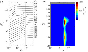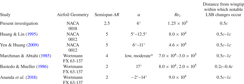



1. Introduction
At low chord Reynolds numbers, the lift to drag ratio of lifting surfaces is often substantially reduced by laminar boundary layer separation from the suction surface (Carmichael Reference Carmichael1981). The wings of small unmanned aerial vehicles and the blades of low pressure gas turbines commonly operate in this flow regime (Lissaman Reference Lissaman1983; Mueller & DeLaurier Reference Mueller and DeLaurier2003; Hodson & Howell Reference Hodson and Howell2005), characterised by the chord Reynolds number  $Re_c<5\times 10^5$ (Carmichael Reference Carmichael1981).
Separation of a laminar boundary layer results in the formation of a separated laminar shear layer near the wing surface. If the laminar shear layer transitions to turbulence, the ensuing strong velocity fluctuations increase the rate of momentum transfer with the external flow, which often leads to flow reattachment in the time-average sense (O'Meara & Mueller Reference O'Meara and Mueller1987). The resulting recirculating flow region confined between the mean separation and reattachment locations is commonly referred to as a laminar separation bubble (LSB) (Tani Reference Tani1964). If transition within the separated laminar shear layer is delayed, reattachment may fail to occur, resulting in a severe reduction in lift and increase in drag (Carmichael Reference Carmichael1981). For this reason, early studies of LSBs, such as those of Gaster (Reference Gaster1967) and Horton (Reference Horton1968), focused on predicting conditions under which separation occurs without reattachment or a relatively small LSB expands into a large one, leading to a sudden performance degradation.
The two-dimensional mean LSB structure, originally proposed by Horton (Reference Horton1968), is presented in figure 1. Joining the mean separation and reattachment points is the mean dividing streamline, defined as the locus of points under which the net streamwise mass flux is zero. Below the dividing streamline is the recirculation region, which can be divided into the dead-air region in the forward part of the bubble and the reverse flow vortex in the aft portion (Horton Reference Horton1968). The transition point is commonly defined near the location of maximum LSB height, where the turbulent shear layer begins to turn towards the wing surface and a substantial surface pressure recovery begins (Brendel & Mueller Reference Brendel and Mueller1988; Boutilier & Yarusevych Reference Boutilier and Yarusevych2012b).
Structure of two-dimensional mean LSB proposed by Horton (Reference Horton1968).

Building on the early research that focused largely on the time-average structure of LSBs, the transition process in LSBs has been the focus of many subsequent investigations. The initial amplification of small amplitude disturbances in LSBs has been shown to agree well with predictions from linear stability theory (Michalke Reference Michalke1991; Lin & Pauley Reference Lin and Pauley1996; Boutilier & Yarusevych Reference Boutilier and Yarusevych2012b). Watmuff (Reference Watmuff1999) experimentally studied the amplification of an impulsive disturbance in an LSB using phased-averaged hot-wire measurements. In the separated shear layer, a cat's eye pattern was observed in the phase-averaged velocity field, which is typical of the Kelvin–Helmholtz instability mechanism. Diwan & Ramesh (Reference Diwan and Ramesh2009) conducted linear stability analysis of velocity profiles measured both upstream and downstream of the separation point of an LSB formed on a flat plate subjected to an adverse pressure gradient. They concluded that disturbance amplification in an LSB begins upstream of separation, initially through the amplification of Tollmien–Schlichting waves in the attached boundary layer. As these waves convect into the separated shear layer, the Tollmien–Schlichting instability mechanism is gradually superseded by the inviscid Kelvin–Helmholtz instability as the primary means for disturbance amplification.
The continuity of the development of instabilities from the attached into the separated flow regions has been subsequently supported by numerical (Marxen et al. Reference Marxen, Kotapati, Mittal and Zaki2015) and experimental studies (Michelis, Yarusevych & Kotsonis Reference Michelis, Yarusevych and Kotsonis2018). As disturbances become amplified in the separated shear layer, nonlinear effects eventually cause the shear layer to roll up near the location of maximum bubble height (Brendel & Mueller Reference Brendel and Mueller1988; Diwan & Ramesh Reference Diwan and Ramesh2009). The formation and subsequent shedding of roll-up vortices in the separated shear layer has been linked to the increase in wall-normal momentum transfer that leads to mean flow reattachment at the aft part of the LSB (Brendel & Mueller Reference Brendel and Mueller1988; Rist, Lang & Wagner Reference Rist, Lang and Wagner2004; Yarusevych, Sullivan & Kawall Reference Yarusevych, Sullivan and Kawall2009; Lengani et al. Reference Lengani, Simoni, Ubaldi, Zunino and Bertini2017a). At low free-stream turbulence intensities, shear layer roll-up is largely two-dimensional, with the resulting vortices initially possessing a high degree of spanwise coherence (Kirk & Yarusevych Reference Kirk and Yarusevych2017). In contrast, at higher turbulence intensities, shear layer roll-up vortices occur with greater distortions (Burgmann, Dannemann & Schröder Reference Burgmann, Dannemann and Schröder2008; Hosseinverdi & Fasel Reference Hosseinverdi and Fasel2019), and form further upstream due to higher initial disturbance amplitudes (Simoni et al. Reference Simoni, Lengani, Ubaldi, Zunino and Dellacasagrande2017). The interactions and breakdown of shear layer vortices into three-dimensional turbulence is the focus of ongoing research (Rist, Maucher & Wagner Reference Rist, Maucher and Wagner1996; Marxen, Lang & Rist Reference Marxen, Lang and Rist2013; Lengani et al. Reference Lengani, Simoni, Ubaldi, Zunino and Bertini2017a). Multiple types of secondary instabilities have been proposed to explain the breakdown of two-dimensional shear layer vortices into fully developed turbulence, including global instability leading to bifurcation of the LSB topology (Rodríguez & Theofilis Reference Rodríguez and Theofilis2010), elliptical instability of the roll-up vortices (Marxen et al. Reference Marxen, Lang and Rist2013) and instability in the braid region between vortices (Marxen et al. Reference Marxen, Lang and Rist2013). Regions of absolute inviscid instability (Rodríguez, Gennaro & Juniper Reference Rodríguez, Gennaro and Juniper2013), and the superposition of oblique and normal disturbance waves (Michelis et al. Reference Michelis, Yarusevych and Kotsonis2018) have also been identified as possible causes of the generation of three-dimensional turbulence.
In the overwhelming majority of studies on LSBs, attention has been focused on nominally two-dimensional steady flows, such as on airfoils or flat plates outside of end effects. However, in most industrial settings where LSBs occur, such as on aircraft wings or turbine blades, end effects are present and substantial portions of the flow are strongly three-dimensional. Furthermore, small unmanned air vehicles that operate at low chord Reynolds numbers are often designed with relatively low aspect ratio wings to minimise overall aircraft size (Mueller & DeLaurier Reference Mueller and DeLaurier2003). Notably, wingtip vortices can produce large regions of three-dimensional flow over low aspect ratio wings, influencing the formation of laminar separation bubbles (Ananda, Sukumar & Selig Reference Ananda, Sukumar and Selig2015; Chen, Bai & Wang Reference Chen, Bai and Wang2016). The present study is focused on the development of LSBs in such practical configurations, and a more detailed overview of the relevant prior investigations is provided here.
Marchman & Abtahi (Reference Marchman and Abtahi1985) studied the lift and drag forces on a full span finite wing with an aspect ratio ( $AR$) of
 $8$ between
 $Re_c=7\times 10^4$ and
 $3\times 10^5$. They observed a clockwise stall hysteresis loop in the lift coefficient caused by laminar separation on the suction surface, similar to the hysteresis loop observed on the same Wortmann FX 63-137 two-dimensional airfoil section by Huber & Mueller (Reference Huber and Mueller1987). The surface oil flow visualisation of Marchman & Abtahi (Reference Marchman and Abtahi1985) confirmed the presence of an LSB on the wing which was essentially two-dimensional, except within one chord length from the wingtip, where three-dimensional flow patterns could be inferred. Two-dimensional behaviour of the LSB on the inboard portion of a finite wing was also observed by Bastedo & Mueller (Reference Bastedo and Mueller1986) using surface pressure measurements at several spanwise locations on a semispan wing of
 $AR=2$. The chordwise pressure distributions on the semispan wing were found to be equivalent to the chordwise pressure distributions on the same two-dimensional airfoil section at an equivalent effective angle of attack over the inner
 $80\,\%$ of the wingspan.
In the Reynolds-averaged Navier–Stokes simulation performed by Chen, Qin & Nowakowski (Reference Chen, Qin and Nowakowski2013) of a semispan cambered thin plate wing of aspect ratio  $AR=6$ at a Reynolds number of
 $Re_c=6\times 10^4$, the separation and reattachment locations of the LSB were also relatively constant along the span away from the wingtip. The LSB on the cambered thin plate wing initially formed near the wing root and expanded along the wingspan as the angle of attack was increased. Spanwise flow occurred within the recirculation region of the LSB, with the strongest spanwise flow occurring near the wingtip.
Horton (Reference Horton1968) experimentally studied the influence of spanwise flow on an LSB forming on a nominally infinite swept wing. The mean recirculation region of the LSB on the infinite swept wing contained substantial spanwise flow forming a helical vortex. Horton (Reference Horton1968) found that bubble bursting on the infinite swept wing could be predicted by applying his bursting criteria for two-dimensional LSBs to the component of velocity perpendicular to the leading edge, confirming independence between the chordwise and spanwise flow for the range of Reynolds numbers and sweep angles considered. Although no substantial changes to LSB behaviour on infinite swept wings was observed by Horton (Reference Horton1968), the flow field over finite wings is non-uniform in the spanwise direction, which may cause LSB behaviour near a wingtip to deviate from the trends seen on nominally two-dimensional geometries.
Toppings, Kurelek & Yarusevych (Reference Toppings, Kurelek and Yarusevych2021) employed particle image velocimetry (PIV) and surface pressure measurements on a semispan wing of  $AR=2.5$. They observed that the equivalence of the LSB on a finite wing at a given spanwise location and the flow over a two-dimensional airfoil at an effective angle of attack was only valid more than one chord length (c) away from the wingtip, even though the external streamlines did not display substantial spanwise flow at spanwise distances greater than
 $0.5c$ from the wingtip. However, changes in the effective angle of attack along the span of the wing were not observed to cause changes in the locations of separation and reattachment. Instead, the separation and reattachment locations remained at the locations corresponding to the effective angle of attack of the wing root. Furthermore, shear layer vortex shedding occurred in a largely two-dimensional fashion at an approximately constant frequency over the inner
 $80\,\%$ of the wingspan, matching the frequency expected at the effective wing root angle of attack. In a numerical simulation of a plunging semispan wing of
 $AR=3$ with a suction surface LSB, Garmann & Visbal (Reference Garmann and Visbal2017) also observed the formation of leading edge shear layer vortices with a high degree of spanwise uniformity.
Prior flow visualisations and quantitative measurements have shown that LSB formation on the inboard portion of finite wings is largely two-dimensional. However, spanwise changes in LSB behaviour begin to occur near the wingtip which do not occur in two-dimensional flow geometries. Although Toppings et al. (Reference Toppings, Kurelek and Yarusevych2021) concluded that local changes in effective angle of attack did not affect the location of LSB formation up to the minimum distance of  $0.5c$ from the wingtip considered in their study, Bastedo & Mueller (Reference Bastedo and Mueller1986) reported that a downstream shift in separation and reattachment lines occurred on the outboard portion of their finite wing, and concluded that this was a result of the reduction in effective angle of attack near the wingtip. Genç et al. (Reference Genç, Özkan, Özden, Kiriş and Yildiz2018) also reported a similar downstream curvature of the LSB separation and reattachment locations on full span wings of
 $AR=1$ and
 $AR=3$.
The three-dimensional flow near the tip of a finite wing with an LSB was further investigated by Awasthi, Moreau & Doolan (Reference Awasthi, Moreau and Doolan2018) on a semispan wing of  $AR=0.5$, using surface oil flow visualisation and hot-wire and Pitot tube velocity measurements. Substantial spanwise flow was seen near the wingtip in oil flow visualisations of the LSB on the suction surface at moderate angles of attack. They also reported that the separation line of the LSB remained nearly parallel to the leading edge, while the reattachment line displayed greater three-dimensionality, moving upstream near the wingtip. Between the LSB and the flow region dominated by the wingtip vortex, Awasthi et al. (Reference Awasthi, Moreau and Doolan2018) observed a substantial reduction in boundary layer thickness and reduction in wake velocity deficit, suggesting an absence of laminar separation and a reduction of the streamwise adverse pressure gradient in this region. However, it is unclear from time-averaged point measurements how these changes are related to the dynamics of LSB transition near the wingtip.
The topology of low aspect ratio three-dimensional separation bubbles was studied by Kremheller & Fasel (Reference Kremheller and Fasel2010) using a three-dimensional displacement body to impose a streamwise and spanwise pressure gradient on a flat plate, producing a three-dimensional LSB. Unlike the mean LSB topology in figure 1, this type of three-dimensional LSB was observed to exchange fluid between the recirculation region and the surrounding flow. According to the classification of surface flow topologies of Perry et al. (Reference Perry, Hornung, Perry and Hornung1984), the topological structure of the three-dimensional LSB on the flat plate was an owl face of the first kind, with two counter-rotating foci at opposite ends of the unstable manifold emanating from a saddle point in the symmetry plane (Kremheller & Fasel Reference Kremheller and Fasel2010). This separation pattern was also observed in the oil flow visualisations of Liu & Hsiao (Reference Liu and Hsiao2014), PIV measurements of Gresham, Wang & Gursul (Reference Gresham, Wang and Gursul2010) and numerical simulations of Chen et al. (Reference Chen, Bai and Wang2016) on thin low aspect ratio wings. These studies have revealed mean surface topologies for LSBs on low aspect ratio wings at low Reynolds numbers, but the relationship between three-dimensional LSB structure and dynamics has not been investigated in detail.
Although three-dimensional LSBs on finite wings have been found analogous to LSBs forming on two-dimensional airfoils away from wingtips, wingtip vortices are known to inhibit laminar separation and cause highly three-dimensional flow in their vicinity (Marchman & Abtahi Reference Marchman and Abtahi1985; Bastedo & Mueller Reference Bastedo and Mueller1986; Shields & Mohseni Reference Shields and Mohseni2012; Mizoguchi & Itoh Reference Mizoguchi and Itoh2013; Ananda et al. Reference Ananda, Sukumar and Selig2015; Awasthi et al. Reference Awasthi, Moreau and Doolan2018). Thus, notable changes may be expected to the classical LSB topology and the associated flow development, as speculated in Toppings et al. (Reference Toppings, Kurelek and Yarusevych2021). While previous works involving finite wings have focused primarily on the surface imprints of the attendant three-dimensional flows, the three-dimensional flow fields of LSBs on finite wings remain largely unexplored. A comprehensive description of the three-dimensional topology and the dynamics of LSBs on finite wings is essential to understand how the established characteristics of two-dimensional LSBs manifest in practical flows subjected to three-dimensional wingtip effects. The objective of this study is to characterise the evolution of the LSB on the suction surface of a finite wing from the region of nominally two-dimensional flow to the region of highly three-dimensional flow near the wingtip. The primary focus is on unveiling the mean three-dimensional structure of the LSB, and relating it to the spanwise changes in the shear layer transition process and the associated development of dominant coherent structures. To this end, an experimental investigation was undertaken on a two-dimensional NACA 0018 airfoil model and semispan wing with  $AR=2.5$ at
 $Re_c = 1.25\times 10^5$. Three- and two-component planar PIV measurements were performed in multiple, closely spaced wall-normal planes, as well as in one wall-tangent plane, to reconstruct the three-dimensional velocity field in the region of LSB formation and compare it with the reference case of a nominally two-dimensional LSB on the same geometry. Complementary surface pressure measurements were also conducted at multiple chordwise and spanwise pressure taps. The remainder of the paper is organised as follows. Section 2 describes the experimental set-up, measurement and data processing techniques, § 3 presents the experimental findings, § 4 compares the results of the present study with previous works and § 5 presents the concluding remarks.
2. Methods of investigation
2.1. Model set-up
All measurements were conducted in the recirculating wind tunnel at the University of Waterloo. The test section has a  $0.61\ \textrm {m}\times 0.61\ \textrm {m}$ square cross-section, and is
 $2.44\ \textrm {m}$ long. The free-stream velocity in the test section was set according to a calibration of the pressure drop across the wind tunnel's 9 : 1 contraction. All measurements were conducted at a chord Reynolds number of
 $Re_c=1.25\times 10^5$, which corresponds to a free-stream velocity
 $U_\infty$ of approximately
 $9.5\ \textrm {m}\ \textrm {s}^{-1}$. At this velocity, the turbulence intensity in the empty test section measured using a normal hot-wire probe and low-passed at
 $10$ kHz was less than
 $0.09\,\%$. The integral length scale was calculated to be
 $0.26c$, where
 $c$ is the airfoil chord length.
The anodised aluminium wing model used in this investigation was manufactured with a NACA 0018 airfoil section and a chord length of  $c=0.2\ \textrm {m}$. The wing model was cantilevered from one of the side walls of the test section, with a semispan of
 $0.5\ \textrm {m}$, and an aspect ratio of
 $AR=2.5$. The gap between the flat tip of the wing model and the opposite wall of the test section was
 $0.5c$, verified to be sufficiently large enough to maintain a lift distribution representative of free-flight conditions (Toppings et al. Reference Toppings, Kurelek and Yarusevych2021). The wing model was equipped with
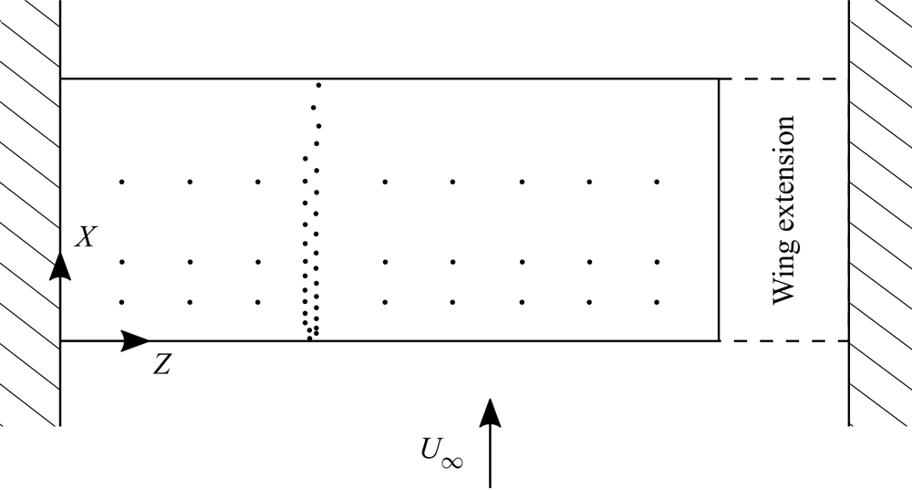
 $89$ static pressure taps arranged in three spanwise rows of nine pressure taps on the suction surface and one chordwise array of 65 pressure taps distributed over the pressure and suction surfaces, with three pressure taps shared between the chordwise and spanwise arrays. Figure 2 shows the location of the pressure taps on the suction surface of the wing model. The three spanwise rows of taps were located at
 $X/c=0.15,0.30,$ and
 $0.60$. The staggered row of chordwise taps was centred at
 $Z/c=0.95$. Surface static pressures were measured using two scanivalve multiplexers connected to two Setra 239 pressure transducers with an input span of
 $\pm 250$ Pa. The uncertainty in surface pressure measurements is estimated to be less than
 $2\,\%$ of the free-stream dynamic pressure. All measurements were conducted at a geometric angle of attack of
 $\alpha =6^\circ$. The angle of attack was set using a digital protractor with a resolution of
 $0.1^\circ$. Repeated surface pressure measurements indicated that the angle of attack could be reliably set within
 $0.2^\circ$. To enable measurements of a two-dimensional NACA 0018 airfoil section using the same model, an extension with a matching NACA 0018 profile was added to the end of the wing so that the model spanned the entire test section from wall to wall (figure 2).
Location of pressure taps on suction surface of wing model. Dashed lines show where the wing extension was installed for two-dimensional airfoil measurements.

2.2. Particle image velocimetry
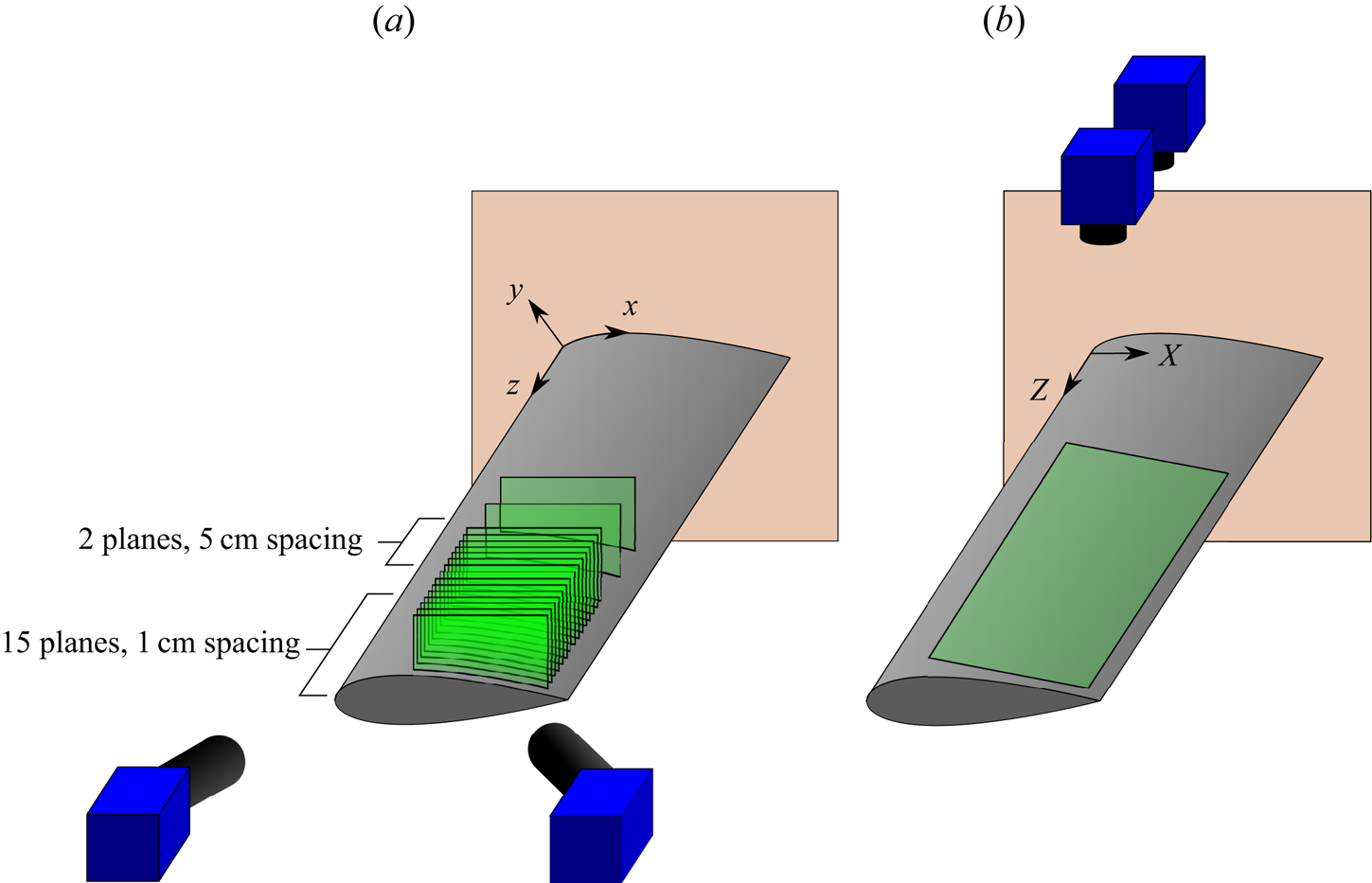
Two configurations of PIV measurements were performed on the flow over the suction surface of the wing and airfoil models (figure 3). The first configuration (figure 3a), referred to as the side-view configuration, was used to measure the three-dimensional velocity field at 17  $x$–
 $y$ planes. Starting from the wingtip, stereo-PIV measurements were taken in planes with
 $0.05c$ (
 $1$ cm) spacing in the
 $Z$ direction from
 $z/c=2.45$ to
 $z/c=1.75$. Two additional stereo-PIV measurement planes were located at
 $z/c=1.50$ and
 $1.25$. Stereo-PIV measurements were also conducted on the two-dimensional airfoil configuration at
 $z/c=1.25,1.50,1.75,1.90$ and
 $2.00$ at same geometric angle of attack of
 $6^\circ$.
PIV measurement arrangement and coordinate axes. (a) Side-view stereo-PIV and (b) top-view PIV.

The second configuration of PIV measurements (figure 3b), referred to as the top-view configuration, was used to further elucidate the spanwise flow development. Here, two cameras were used side by side for two-component velocity measurements over an extended portion of the wing surface.
Table 1 summarises the parameters of the PIV measurement systems used for the side-view and top-view configurations. For both configurations, the flow was seeded with water–glycol fog particles that were illuminated with a Photonics DM20-527 Nd:YLF pulsed laser. For the side-view configuration, particle images were acquired with two LaVision Imager sCMOS  $5.5\ \text {Mpx}$ cameras, equipped with
 $200$ mm fixed focal length Nikon macro lenses and Scheimpflug adapters, in double frame mode at
 $52.35$ Hz. At each plane,
 $1000$ uncorrelated velocity fields were obtained. The forming optics for the light sheet were located approximately
 $8c$ downstream of the wing in the test section, and verified to have no measurable effect on the flow development over the model via surface pressure measurements. From the width of the correlation peaks in the self-calibration correlation maps, the thickness of the light sheet was estimated to be 2 mm (Wieneke Reference Wieneke2005). To compensate for the difference in particle image intensities due to forward and backward scattering, the apertures of the upstream and downstream cameras were set to
 $f/5.6$ and
 $f/4$, respectively. The images from both cameras were cropped to
 $2560\ \text {px}\times 1024\ \text {px}$, yielding a total field of view of approximately
 $0.3c\times 0.08c$. The cameras and the laser optics were positioned using computer-controlled precision traverse stages, with a resolution of
 $0.1$ mm, allowing for a synchronous repositioning of the measurement plane. A target calibration was performed for the first measurement plane, followed by self-calibration (Wieneke Reference Wieneke2005) for each measurement plane. All particle images were pre-processed using a global minimum subtraction followed by pixel intensity normalisation by the average intensity. Particle displacements were then computed using an iterative multi-grid cross-correlation scheme with window deformation (Scarano & Riethmuller Reference Scarano and Riethmuller2000). A window size of
 $16\ \text {px}\times 16\ \text {px}$ with
 $75\,\%$ overlap was used for the final iteration, resulting in a vector pitch of
 $0.10$ mm. The results were accepted if the stereo reconstruction error was less than
 $1\ \text {px}$. Outlier detection and removal was performed on the raw velocity fields using a median filter (Westerweel & Scarano Reference Westerweel and Scarano2005). The resulting stereo-PIV vector fields were interpolated onto the surface attached coordinate system. Particle image acquisition, pre-processing and processing were performed in the LaVision Davis 10 software.
PIV Measurement Parameters.

For the top-view configuration (figure 3b), the laser sheet was formed outside of the test section. Particle images were acquired using the same two sCMOS cameras, equipped with  $50$ mm fixed focal length Nikon macro lenses, in double frame mode at
 $36$ Hz. A total of
 $4488$ velocity fields were obtained. The cameras were placed side by side to capture an expanded spanwise region of the wing at an acceptable spatial resolution. Images from both cameras were cropped to
 $2560\ \text {px}\times 1492\ \text {px}$, and the particle images were pre-processed using a sliding minimum subtraction. Image processing was based on an iterative multi-grid cross-correlation scheme (Scarano & Riethmuller Reference Scarano and Riethmuller2000) with a final window size of
 $24\ \text {px}\times 24\ \text {px}$ and
 $75\,\%$ window overlap, resulting in a vector pitch of
 $0.38$ mm. Outlier detection and removal was performed on the raw velocity fields using a median filter (Westerweel & Scarano Reference Westerweel and Scarano2005). The combined field of view of both cameras was approximately
 $1.57c\times 0.43c$.
The uncertainty due to random errors in the PIV measurements was estimated using the correlation statistics method (Wieneke Reference Wieneke2015). In the side-view configuration, the maximum root-mean-square (r.m.s.) uncertainty occurred in the near wall regions upstream and downstream of the LSB where large velocity gradients occur next to the wing surface. The r.m.s. uncertainties ( $95\,\%$ confidence level) within the LSB in the side-view configuration are approximately
 $2\,\%$,
 $2\,\%$ and
 $5\,\%$ of the free-stream velocity for the streamwise (
 $u$), wall-normal (
 $v$) and spanwise (
 $w$) velocity components, respectively. The total uncertainty in the mean velocity fields, including the uncertainty from calibration, is less than
 $13\,\%$ of the free-stream velocity for all velocity components. The r.m.s. uncertainties (
 $95\,\%$ confidence level) in the top-view configuration were approximately
 $4\,\%$ of the free-stream velocity for both the
 $u$ and
 $w$ velocity components. The uncertainties associated with quantities derived from PIV data were calculated using uncertainty propagation (Moffat Reference Moffat1988), incorporating uncertainties due to random and bias errors.
The coordinate systems used for data presentation are depicted in figures 2 and 3, with the same origin located at the wing root leading edge. The  $X{-}Z$ coordinates are used for the presentation of surface pressure and top-view PIV measurements, with
 $X$ and
 $Z$ aligned along the chord and wing span respectively (figure 2). A surface attached coordinate system (
 $x{-}y{-}z$, figure 3) is used to present the side-view PIV data and associated derived quantities. Streamline and streamsurface generation from the side-view PIV measurements was performed using the fourth-order Runge–Kutta method with linear interpolation of the velocity field.
2.3. Proper orthogonal decomposition
Proper orthogonal decomposition (POD) was used to analyse the development of coherent structures in the flow, using the method of snapshots introduced by Sirovich (Reference Sirovich1987). The POD was performed on the fluctuating velocity fields  $\boldsymbol {u}'_i=\boldsymbol {u}_i-\bar {\boldsymbol {u}}$, where the subscript
 $i$ is the index of a given snapshot. The reconstruction of the velocity field with the results of the POD decomposition takes the form (Legrand, Nogueira & Lecuona Reference Legrand, Nogueira and Lecuona2011a)
 \begin{equation} \boldsymbol{u}_i=\bar{\boldsymbol{u}}+\sum_{n=1}^N a^{(n)}_i\sqrt{E^{(n)}}\boldsymbol{\varPhi}^{(n)},\quad i=1\ldots N,\end{equation}
where  $N$ is the number of snapshots,
 $a^{(n)}_i$ are the temporal coefficients,
 $E^{(n)}$ are the modal energies and
 $\boldsymbol {\varPhi }^{(n)}$ are the spatial POD mode shapes. The POD modes are conventionally sorted in the order of decreasing energy content, with the first mode (
 $n=1$) corresponding to the highest energy content. In flows dominated by the convection of vortices, including LSBs, the prevalent flow structures are captured by paired modes, which have similar energy content and spatial mode topology but shifted in space by one quarter of the characteristic length scale of the structures (van Oudheusden et al. Reference van Oudheusden, Scarano, van Hinsberg and Watt2005; Legrand et al. Reference Legrand, Nogueira and Lecuona2011a; Lengani et al. Reference Lengani, Simoni, Ubaldi and Zunino2014).
In addition, POD can be employed to produce phase-average flow reconstructions (Ben Chiekh et al. Reference Ben Chiekh, Michard, Grosjean and Béra2004; van Oudheusden et al. Reference van Oudheusden, Scarano, van Hinsberg and Watt2005). In a fully deterministic periodic flow characterised solely by a vortex train with constant convective velocity and wavelength, the paired temporal coefficients  $a^{(1)}$ and
 $a^{(2)}$ take the form (Legrand et al. Reference Legrand, Nogueira and Lecuona2011a)
 $$\begin{gather} a^{(1)}_i = \sqrt{2/N}\cos(\varTheta_i), \end{gather}$$
 $$\begin{gather}a^{(2)}_i =\sqrt{2/N}\sin(\varTheta_i), \end{gather}$$
where  $\varTheta _i$ is the phase angle of the vortex shedding cycle for a given snapshot
 $i$. Therefore, the temporal coefficients of the paired modes can be used to sort non-time-resolved data samples according to the phase of the fundamental vortex shedding cycle using the relation
 \begin{equation} \varTheta_i = \tan^{{-}1}\left(\frac{a^{(1)}_i}{a^{(2)}_i}\right). \end{equation}
While POD-based phase averaging is often conducted by binning the velocity snapshots falling within a certain phase angle range (Legrand et al. Reference Legrand, Nogueira, Tachibana, Lecuona and Nauri2011b), the polynomial fitting method of Lengani et al. (Reference Lengani, Simoni, Ubaldi and Zunino2014), was adopted in the present study. It involves applying a least squares fifth-order polynomial fit to the phase-sorted velocity data at each point in space, as illustrated in figure 4. A distinct advantage of the polynomial fitting method is that it provides a continuous relationship between phase angle and velocity at a given point. The obtained velocity–phase relations at each spatial point then allow to reconstruct the phase-averaged velocity field at a desired phase angle.
Phase averaging using polynomial fitting. Streamwise velocity data from top view at  $(X/c,Z/c) = (1.32,0.40)$.

As discussed by Legrand et al. (Reference Legrand, Nogueira, Tachibana, Lecuona and Nauri2011b), for improved accuracy of phase averaging, the cumulative energy of a reference modal pair should exceed  $10\,\%$ of the total energy of velocity fluctuations. Thus, unlike the standard POD performed on the two- or three-component velocity vector measured in a given plane, it is beneficial to do phase reconstruction using POD applied to the most dominant component of velocity fluctuations. In the present study, this was accomplished by using wall-normal fluctuations and streamwise fluctuations for phase averaging of the results obtained in side-view (figure 3a) and top-view (figure 3b) configurations, respectively. The resulting cumulative modal energy of the first two modes for the side-view measurements was over
 $48\,\%$ where distinct shedding was observed for the planes away from the wingtip (
 $z/c\leq 2.15$), as depicted in figure 5(a), which presents the relative energy (
 $E_r$) of the first twenty modes at
 $z/c=1.25$. In the vicinity of the wingtip, the planes were considered for the phase averaging and reconstruction only where the relative cumulative energy of the most energetic mode pair reached
 $10\,\%$. For the top-view measurements, the first two modes captured
 $12\,\%$ of the total fluctuating energy content (figure 5b). The representative spatial mode shapes shown in figure 5 confirm that the most energetic mode pairs exhibit a similar periodic spatial topology, offset by one quarter of a wavelength. Although the first and second most energetic modes from both the side and top views are of a similar order of magnitude as the higher modes, Legrand et al. (Reference Legrand, Nogueira, Tachibana, Lecuona and Nauri2011b) showed that reasonably accurate phase averaging using POD can be performed even when the modal energy of the dominant mode pair is of a similar order of magnitude to the energy of higher modes in multiple types of periodic flows.
Representative relative energy distributions of the first twenty POD modes and spatial distributions of the mode pairs of the velocity fluctuation components used for phase averaging. Grey shaded regions of high noise have been masked. (a) Side view  $z/c = 1.25, v'$ and (b) top view,
 $u'$.

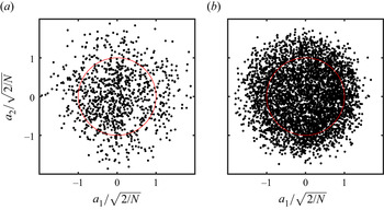
Figure 6 depicts a cross-plot of  $a_1$ and
 $a_2$ used for phase angle determination. Note that
 $1000$ snapshots were used for POD in the side-view planes, while
 $4488$ snapshots were employed for the top view. It can be seen that cycle-to-cycle variations in the vortex shedding process produce a substantial scatter of the experimental data away from the unit circle that represents the distribution expected for a perfectly periodic vortex train, since the energy of higher modes is of a similar order of magnitude (figure 5). The data scatter observed is similar to that of an unforced LSB on a two-dimensional airfoil (e.g. Kurelek Reference Kurelek2021). A convergence study of the POD modal energies was performed, and it was estimated that the relative energy of the most energetic mode pairs was converged to within
 $1\,\%$ and
 $0.1\,\%$ for the side- and top-view configurations, respectively.
Cross-plot of temporal coefficients of POD modes used for phase averaging. Unit circle is shown in red. (a) Side view  $z/c = 1.25$ and (b) top view.

3. Results
The results of this investigation pertain to the LSB forming on the suction surface of a rectangular NACA 0018 semispan wing at an angle of attack of  $\alpha =6^\circ$ and a chord Reynolds number of
 $Re_c = 1.25\times 10^5$. Under these conditions, a typical short LSB (Gaster Reference Gaster1967) forms on the suction surface sufficiently far from the trailing edge to prevent tonal noise emissions (Pröbsting & Yarusevych Reference Pröbsting and Yarusevych2015). PIV is used to reconstruct the three-dimensional structure of the mean LSB and gain insight into the attendant transition process and shear layer vortex shedding. The evolution of the LSB in the spanwise direction is presented from the region of nominally two-dimensional flow at the midspan to the wingtip, where the flow field is highly three-dimensional under the influence of the wingtip vortex.
3.1. Mean flow topology
To demonstrate the mean spanwise changes in the LSB on the wing, a comparison is made with the two-dimensional airfoil. Mean surface pressure measurements on the wing and two-dimensional airfoil are presented in figure 7. The chordwise pressure distributions in figure 7(a) display a plateau downstream of the suction peak, which is characteristic of the dead-air region of the LSB (Horton Reference Horton1968). The plateau is followed by a rapid pressure recovery which indicates the reattachment of the shear layer in the aft portion of the bubble. As expected, tip effects reduce the suction developed by the wing when compared with the two-dimensional airfoil at the same geometric angle of attack of  $\alpha =6^\circ$. At
 $\alpha =5^\circ$, the two-dimensional airfoil produces a chordwise pressure distribution that essentially matches the pressure distribution on the wing at
 $\alpha =6^\circ$ and
 $Z/c = 0.95$, implying that the effective angle of attack of the wing at
 $Z/c = 0.95$ is approximately
 $5^\circ$, as discussed in detail by Toppings et al. (Reference Toppings, Kurelek and Yarusevych2021). Figure 7(b) presents surface pressure measurements from the three rows of spanwise pressure taps for the wing at
 $\alpha =6^\circ$ and for the two-dimensional airfoil at the effective angle of attack of the inboard region (
 $\alpha =5^\circ$). The pressure distribution on the two-dimensional airfoil is essentially uniform in the spanwise direction. On the wing for
 $Z/c<1$, the pressure distribution also does not display significant spanwise gradients. However, for
 $Z/c>1$, a substantial spanwise pressure gradient develops progressively as the wingtip is approached. Figure 7(b) also indicates that the chordwise pressure gradient is reduced near the wingtip.
Surface pressure distributions on the wing and airfoil. (a) Streamwise distribution and (b) spanwise distribution. Symbols in (a) mark measurements common to the streamwise and spanwise distributions. Dotted line in (b) shows the spanwise location of the measurements presented in (a).

Figure 8 presents contours of streamwise velocity on the wing at  $\alpha =6^\circ$ at
 $z/c=1.25$ and on the two-dimensional airfoil at both the effective angle of attack of
 $5^\circ$ and the geometric angle of attack of
 $6^\circ$. Also shown is the streamwise displacement thickness
 $\delta ^*_x$, defined as
 $\delta ^*_x=\int _{0}^{\delta }(1-u/u_e){\textrm {d} y}$, where
 $u_e$ is the local edge velocity and
 $\delta$ is the boundary layer thickness. The streamwise displacement thickness was verified to closely follow the wall-normal height of the inflection point in the separated shear layer. Since the calculation of integral boundary layer parameters in three-dimensional flows requires resolving the boundary layer velocity field starting from the upstream stagnation point, planar estimations of the displacement and momentum thickness (
 $\delta ^*_x$ and
 $\theta _x$) based on a two-dimensional approximation are used here.
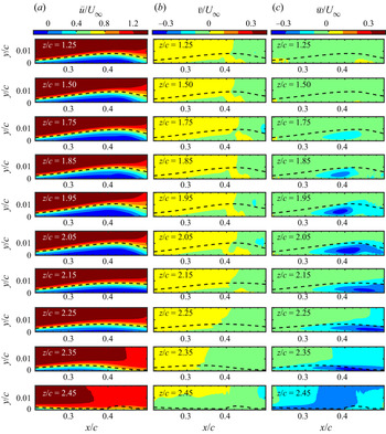
Contours of mean streamwise and spanwise velocity on the wing and airfoil. Dashed line: streamwise displacement thickness. Panel (b) is based on data from Toppings et al. (Reference Toppings, Kurelek and Yarusevych2021)

The results in figure 8 reveal the presence of a typical LSB for all the cases shown. The extent of the mean reverse flow region (depicted by the darkest blue contour level) on the wing (figure 8a) and on the two-dimensional airfoil at the same effective angle of attack (figure 8b) show no substantial differences, confirming the close similarity between the mean LSB sufficiently far away from the wingtip and that on the airfoil at the matching effective angle. Compared with the airfoil at the same geometric angle of attack (figure 8c), the LSB location on the wing (figure 8a) is shifted downstream due to the reduction in effective angle of attack, which reduces the adverse pressure gradient and delays separation (Bastedo & Mueller Reference Bastedo and Mueller1986; Boutilier & Yarusevych Reference Boutilier and Yarusevych2012a; Herbst, Hain & Kähler Reference Herbst, Hain and Kähler2020).
Figure 9 highlights the spanwise changes in the mean velocity field towards the wingtip based on a representative subset of measurement planes. From  $z/c=1.25$ to
 $z/c=2.05$, the streamwise velocity contours in figure 9(a) show no substantial changes in the streamwise extent of the reverse flow region. Within this spanwise region, the LSB position and length are in close agreement with those on the two-dimensional airfoil at the effective angle of attack (figure 8b). At
 $z/c=2.15$, the LSB moves downstream, and the reverse flow region can be seen to extend beyond the maximum downstream extent of the field of view. Closer to the wingtip, at
 $z/c=2.25$, the full streamwise extent of the reverse flow region is again captured within the field of view, and its length and height diminish notably. Eventually, at and beyond
 $z/c=2.35$, no reverse flow is detected. This is accompanied by a notable decrease in boundary layer thickness, which is due to a significant downwash induced by the wingtip vortex evidenced by the negative wall-normal component of mean velocity in figure 9(b) at
 $z/c=2.45$.
Mean velocity contours in selected  $x$–
 $y$ planes. Dashed line: streamwise displacement thickness.

The spanwise velocity contours in figure 9(c) reveal the presence of substantial spanwise flow in the LSB, reflecting the increased three-dimensionality of the flow field near the wingtip. As expected for a finite wing, the spanwise flow over the suction surface occurs in the negative  $z$ direction towards the wing root. Notably, the recirculation region of the LSB near the wingtip contains substantially higher spanwise velocities than the surrounding flow, indicating that the recirculation region is influenced by the spanwise pressure gradient. At
 $z/c=1.25$, where the LSB on the wing is similar to that on the two-dimensional airfoil at the same effective angle of attack, the magnitude of spanwise flow does not exceed
 $0.1U_\infty$. However, over the range
 $1.95< z/c<2.15$ the magnitude of spanwise velocities in the reverse flow region exceed
 $0.3U_\infty$. The increased strength of the spanwise flow on this part of the span coincides with major spanwise changes in the length and height of the reverse flow region visible in figure 9(a). At
 $z/c=2.45$, substantial spanwise flow in the negative
 $z$ direction occurs across the entire field of view because of the proximity of the wingtip vortex core.
In two-dimensional flows, the locations of boundary layer separation and reattachment are traditionally defined as points where skin friction vanishes (Prandtl Reference Prandtl1904). However, in three-dimensional flows, the skin friction may be non-zero at locations of separation and reattachment (Tobak & Peake Reference Tobak and Peake1982; Délery Reference Délery2001). The topological theory of three-dimensional separation requires that separation lines be unstable manifolds of saddle points in the limiting streamline field, whereas reattachment lines be stable manifolds of saddle points (Surana, Grunberg & Haller Reference Surana, Grunberg and Haller2006). However, some studies have asserted that separation and reattachment can occur along limiting streamlines that do not connect to saddle points (Wang Reference Wang1970; Wu et al. Reference Wu, Tramel, Zhu and Yin2000), and this type of separation is commonly referred to as cross-flow separation.
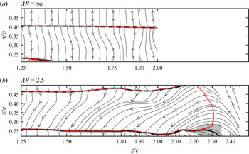
Figures 10(a) and 10(b) present limiting streamlines on the two-dimensional airfoil and wing, respectively. Limiting streamlines were calculated from the velocity gradient at the surface using a third-order polynomial fit to the ten velocity vectors nearest to the surface at each  $(x,z)$ location. Note that due to the higher effective angle of attack of the two-dimensional airfoil, the LSB is located farther upstream in comparison with the finite wing at the same geometric angle of attack. Although the separation line is located just outside of the field of view for the two-dimensional configuration, the results show a strongly uniform mean reattachment and nearly two-dimensional limiting streamlines (figure 10a). This is in agreement with spanwise surface pressure measurements, which show spanwise variations below
 $6\,\%$ of the spanwise average in the reverse flow region (
 $X/c=0.3$, figure 7b).
Limiting streamlines. Thick solid and dashed lines: mean separation and reattachment lines, respectively; red line:  $C_{fx}=0$ contour. Vertical tick marks indicate spanwise locations of side-view measurement planes. Shaded regions indicate uncertainty in separation and reattachment line estimates.

On the wing (figure 10b), the separation and reattachment lines have been heuristically identified as the attractor and repellor of nearby limiting streamlines in the separation and reattachment regions, respectively. Because the separation line of the LSB on the wing does not emanate from a saddle point, it is classified as a cross-flow separation (Wang Reference Wang1970; Tobak & Peake Reference Tobak and Peake1982). Similar to the results of numerical simulations of cross-flow separation on an ogive cylinder by Yates & Chapman (Reference Yates and Chapman1988), a well-defined onset of separation cannot be identified at the outboard end of the LSB ( $2.10\leq z/c \leq 2.35$, figure 10b), where the streamlines gradually approach a common envelope. The separation and reattachment lines obtained from the limiting streamline topology are also compared with the contour of zero streamwise wall shear stress (
 $C_{fx}=0$) in figure 10(b). It can be seen that the contour of
 $C_{fx}=0$ closely follows the separation and reattachment lines across the majority of the LSB. Only in the tip region, where the limiting streamlines are oriented primarily in the spanwise direction, the zero streamwise wall shear stress contour begins to deviate from the separation line. This suggests that the two-dimensional definition of separation and reattachment based on zero streamwise skin friction can be used to identify the location and streamwise extent of an LSB on a finite wing, except for the immediate proximity of the wingtip.
The limiting streamlines on the wing in figure 10(b) reveal that the near-surface flow is largely spanwise uniform in the inboard region ( $1.25 \leq z/c \leq 1.85$), despite a notable spanwise flow component within the LSB. As the wingtip is approached, the separation line remains at a nearly consistent
 $x/c$ location before curving upstream at
 $z/c\approx 2.30$, whereas the reattachment line moves downstream and exits the field of view. The limiting streamlines within the LSB display a progressively increasing spanwise orientation with increasing
 $z/c$, consistent with the spanwise flow observed in figure 9(c), suggesting that fluid enters into the LSB at its outboard end. For
 $z/c>2.25$, the limiting streamlines reorient into the positive streamwise direction due to the influence of the wingtip vortex, which suppresses boundary layer separation (Lamar Reference Lamar1974; Torres & Mueller Reference Torres and Mueller2004).
The overall limiting streamline field displays a strong similarity to the qualitative flow visualisations by Huang & Lin (Reference Huang and Lin1995), Yen & Huang (Reference Yen and Huang2009), and Ananda, Selig & Deters (Reference Ananda, Selig and Deters2018) of LSBs on finite wings. A downstream shift in LSB reattachment lines near the tips of finite wings was also reported from the flow visualisations of Marchman & Abtahi (Reference Marchman and Abtahi1985), Bastedo & Mueller (Reference Bastedo and Mueller1986) and Genç et al. (Reference Genç, Özkan, Özden, Kiriş and Yildiz2018). It is important to note that this behaviour, expected from the reduction in the effective angle of attack (Bastedo & Mueller Reference Bastedo and Mueller1986), is constrained to the relative vicinity of the wingtip ( $z/c>2.15$, figure 10b). For comparison, within
 $1.25\leq z/c \leq 2.15$ where the effective angle of attack changes from approximately
 $5^\circ$ to
 $3^\circ$ (Toppings et al. Reference Toppings, Kurelek and Yarusevych2021), an LSB on a two-dimensional wing would move downstream by approximately
 $0.15c$ (Boutilier & Yarusevych Reference Boutilier and Yarusevych2012a), i.e. approximately
 $75\,\%$ of the present bubble length. Thus, the spanwise variations seen in the LSB extent and position over the majority of the span are significantly lower than those expected from the changes in the effective angle of attack, and the bubble appears to settle on a configuration driven by the effective angle at the wing root, except in the proximity of the wingtip.
Figure 10(b) also reveals a distinct change in direction of the limiting streamlines at approximately  $x/c=0.40$, which roughly demarcates the fore and aft portions of the LSB (i.e. the dead-air region and mean reverse flow vortex, respectively, figure 1). The limiting streamlines in the forward part of the bubble are directed more strongly in the spanwise direction, similar to the numerical simulations of Chen et al. (Reference Chen, Qin and Nowakowski2013). Because the skin friction within the LSB has a negative
 $z$ component, the streamwise gradient in the spanwise flow magnitude implies that the recirculating flow within the LSB follows a helical path which is similar to LSBs on nominally infinite swept wings (Horton Reference Horton1968).
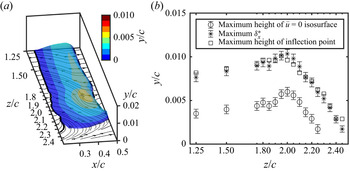
Although the limiting streamline field is in qualitative agreement with previous surface flow visualisations on finite wings at low Reynolds number, resolving the attendant three-dimensional flow field is essential to reconstruct the bubble topology and understand the mechanisms by which the observed surface patterns form. Figure 11(a) presents an isosurface of zero streamwise velocity ( $\bar {u}=0$) constructed from the side-view measurements that illustrates the three-dimensional shape of the LSB on the wing. The results show that the streamwise bounds of the reverse flow region closely follow the separation and reattachment lines determined from the limiting streamline topology. At the outboard end of the LSB, the reverse flow region thickness reduces, and no reverse flow is eventually detected for
 $z/c>2.30$. Beyond this spanwise location, downwash from the wingtip vortex causes the boundary layer to remain attached to the wing surface.
(a) The  $\bar {u}=0$ isosurface. Contour colours indicate normal distance from wing surface. Thin solid lines: limiting streamlines; thick solid line: separation line; thick dashed line: reattachment line. (b) Maximum height of
 $\bar {u}=0$ isosurface, maximum
 $\delta ^*_x$, and maximum height of shear layer velocity profile inflection point.

A quantitative analysis of the changes in the wall-normal extent of the LSB along the span is facilitated by figure 11(b). The spanwise variation of maximum thickness of the  $\bar {u}=0$ isosurface is presented with the maximum streamwise displacement thickness. The latter is shown to closely follow the maximum height of the inflection point in the core of the shear layer. All three parameters vary gradually in the inboard region (
 $1.25 \leq z/c \leq 1.85$). However, a notable increase in the bubble height is observed towards
 $z/c\approx 2.00$, where an increase in both the maximum height of the reverse flow region and streamwise displacement thickness takes place, which agrees with the trend reported by Toppings et al. (Reference Toppings, Kurelek and Yarusevych2021). For
 $z/c>2.00$, a gradual decrease in LSB thickness occurs, until reverse flow is no longer observed in the tip region for
 $z/c>2.30$. The accompanying reduction in displacement thickness is consistent with the findings of Awasthi et al. (Reference Awasthi, Moreau and Doolan2018), who observed a substantial reduction in boundary layer thickness towards the tip of an
 $AR=0.5$ semispan wing.
Based on the observed changes in mean flow topology along the span, three characteristic regions can be identified. The inboard region is located within  $1.25\leq z/c \leq 1.85$ and characterised by nearly spanwise uniform LSB development. The tip region is confined to
 $z/c>2.25$, where the flow is strongly influenced by three-dimensional tip effects, and characteristic LSB features are no longer observed. Between these regions, there is an intermediate region (
 $1.85 < z/c \leq 2.25$), where the thickness of the LSB changes substantially and strong spanwise flow occurs within the reverse flow region.
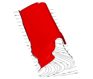
To visualise the three-dimensional shape of the separation bubble, streamsurfaces of separation and reattachment were constructed from the side-view PIV data and are presented in figure 12. The separation surface is formed by the downstream advection of the separation line (Hultquist Reference Hultquist1992). Figure 12(a) shows that the LSB on the wing is an open bubble. Instead of forming a closed surface, the outboard portion of the separation surface is swept towards the wing root by spanwise flow, and fluid enters the LSB at its outboard open end. This is further substantiated by the trajectory of the reattachment surface in figure 12(b), which is the streamsurface that emanates from the reattachment line in reverse time (Surana et al. Reference Surana, Grunberg and Haller2006). Within the intermediate region, the reattachment surface passes over the separation surface and extends farther upstream ( $2.10 \leq z/c \leq 2.25$), indicating that fluid is drawn into the LSB from above and outboard of the separation surface. Farther from the wingtip, the separation and reattachment surfaces approach the same shape, as indicated by the small segment of the reattachment surface near
 $z/c=1.50$ that closely follows the outside of the separation surface. The convergence of the two streamsurfaces in the inboard region of the wing suggests that the bubble topology in
 $x$–
 $y$ planes approaches that of the closed two-dimensional separation bubble depicted in figure 1 away from the wingtip.
Streamsurfaces of separation (red) and reattachment (black). Thin lines: limiting streamlines; thick solid line: separation line; thick dashed line: reattachment line. Insets illustrate the relative position of separation and reattachment streamsurfaces in  $x$–
 $y$ planes. (a) Separation surface and (b) separation and reattachment surfaces.

Because the separation and reattachment surfaces are everywhere tangent to the velocity field, there is zero mass flux across both surfaces. However, as demonstrated by the numerical simulations of Rodríguez & Theofilis (Reference Rodríguez and Theofilis2010), this does not preclude inflows or outflows from the recirculation region of the LSB in the  $x$ direction. This is illustrated in the inset plots of figure 12 which present schematics of the intersection of the dividing streamsurfaces with two-dimensional
 $x$–
 $y$ planes. Near
 $z/c=2.10$, the reattachment surface extends upstream, passing above the separation surface, which allows fluid to enter into the mean reverse flow vortex. In contrast, near
 $z/c=1.90$, the separation surface extends downstream, passing above the reattachment surface, which allows fluid to exit the mean reverse flow vortex. Since the accumulated integration errors in streamsurface calculation and the limited spatial resolution of the PIV measurements make it difficult to quantify the small inflows/outflows based on the calculated separation and reattachment surfaces, a control volume analysis was employed to more precisely determine where fluid enters and exits the three-dimensional open LSB.
The planar control volume analysis was applied to the stereoscopic velocity data from the spanwise region where an LSB is fully captured within the field of view of  $x$–
 $y$ measurement planes (
 $1.25\leq z/c \leq 2.10$). The definition of the planar control volume at
 $z/c=1.25$ is shown in figure 13(a), and the control volume boundaries at all other planes are located at the same
 $x/c$ and
 $y/c$ locations. The control volume boundary was placed around the aft portion of the LSB containing the reverse flow vortex (figure 1), where notable changes take place in the spanwise flow (figure 9b).
Control volume mass balance: (a) control volume superimposed on the LSB outline at  $z/c=1.25$. (b) terms (1) and (2) from (3.1).

The conservation of mass for the planar control volume in an incompressible flow can be expressed as

where  $A$ is the area of the planar control volume bounded by
 $l$ and
 $\hat {\boldsymbol {n}}$ is the outward unit normal vector on the boundary. Term (1) represents the net in-plane outflow of fluid through the boundaries of the planar control volume due to the in-plane components (
 $u$ and
 $v$) of the mean velocity (
 $\bar {\boldsymbol {u}}$) at the control volume boundaries. Term (2) represents the net out-of-plane outflow of fluid due to spanwise gradients in spanwise velocity, which is equal to the derivative of the mean bound spanwise volume flow rate (
 $\bar {\dot {V}}$) with respect to
 $z$.
Figure 13(b) presents the values of terms (1) and (2) for each of the planar control volumes. The observed changes in the spanwise gradient of the spanwise volume flow rate, and consequently term (2) in (3.1), necessitate changes in the net in-plane outflow (term (1), (3.1)) through the control volume boundaries. It can be seen that, at a given spanwise location, the two terms add to zero to within the experimental uncertainty. Of particular interest, however, are the signs of the respective terms, distinguishing between inflow and outflow.
The last outboard plane that captures the full extent of the LSB is located at  $z/c=2.10$, where the LSB topology experiences notable changes due to the proximity of the wingtip, including the reduction of the bubble height and downstream movement of the reattachment location (figure 11). In figure 13(b), term (1) is negative at this location, reflecting the inflow into the open end of the LSB. As the gradient of the spanwise volume flow rate inside the LSB diminishes inboard, in-plane outflow (i.e. positive term (1)), is eventually attained, peaking in the intermediate region and then gradually decreasing towards the expected zero value for the nearly two-dimensional flow in the inboard region. The spanwise region of maximum in-plane outflow from the planar control volume matches that of maximum LSB thickness in figure 11(b). Thus, the increase in LSB thickness in the intermediate region is attributed to changes in the mass exchange balance between the LSB and the surrounding fluid driven by the spanwise flow across the open end of the LSB. Consequently, the strong three-dimensional flow induced by the wingtip vortex not only causes open LSB formation and attached flow near the tip, but also induces notable spanwise changes to the LSB position, length, and height in the intermediate region.
3.2. Laminar to turbulent transition
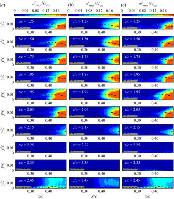
Due to the critical role of shear layer transition in determining the overall mean LSB topology, the observed spanwise variations in the mean flow of the three-dimensional LSB on the wing are expected to be linked to changes in the transition process. The evolution of velocity perturbations in the shear layer is explored in figure 14, which presents contours of r.m.s. velocity fluctuations. For the inboard region (e.g. at  $z/c=1.25$), the results reveal the progressive amplification of streamwise velocity fluctuations along the core of the separated shear layer, which is most prominent around the maximum height location. The attendant flow transition leads to mean flow reattachment, where saturation of velocity fluctuations is observed, agreeing with previous studies (Boutilier & Yarusevych Reference Boutilier and Yarusevych2012b; Marxen et al. Reference Marxen, Lang and Rist2013). Near the
 $x/c$ location of maximum bubble height, identifiable from the streamwise displacement thickness plots (dashed lines), the streamwise velocity fluctuation contours (figure 14a) exhibit three peaks, with the middle one aligned along the core of the shear layer, a structure expected from other experiments in separated shear flows (Dovgal, Kozlov & Michalke Reference Dovgal, Kozlov and Michalke1994; Häggmark, Bakchinov & Alfredsson Reference Häggmark, Bakchinov and Alfredsson2000) and linear stability predictions (Michalke Reference Michalke1991; Marxen et al. Reference Marxen, Kotapati, Mittal and Zaki2015). The wall-normal velocity fluctuations (figure 14b) for the inboard planes display a single peak along the trajectory of the separated shear layer, consistent with the formation of shear layer vortices. The observed trends persist in all measurement planes for
 $z/c\lesssim 2.00$ and are similar to those expected for a two-dimensional LSB (Lengani et al. Reference Lengani, Simoni, Ubaldi, Zunino and Bertini2017b). The spanwise velocity fluctuations captured in the present investigation (figure 14c) offer a novel insight into the progression of the last stages of the transition process, where onset of spanwise fluctuations is expected. It can be seen that similar levels of spanwise velocity fluctuations are achieved farther downstream compared with either streamwise or wall-normal components. As will be discussed later, these arise from spanwise deformations and subsequent breakdown of dominant shear layer vortices in the aft portion of the LSB.
The r.m.s. velocity contours. Dashed line: streamwise displacement thickness. Masked flow area within  $0.2< x/c<0.3$ pertains to region of relatively high random errors near the wall.

Significant changes in the development of shear layer velocity fluctuations take place in the intermediate region for  $z/c>2.00$ (figure 14). Most notably, a progressive downstream shift of the transition process can be seen between
 $z/c=2.05$ and
 $2.25$, and no significant velocity fluctuations are observed within the field of view in the tip region at
 $z/c=2.25$ and
 $2.35$. Figure 15(a) presents a convenient comparison basis for the assessment of spanwise variations in turbulent kinetic energy (TKE) at the core of the shear layer superimposed on the mean separation and reattachment lines. Also presented is the streamwise location of maximum shape factor
 $H_x=\delta ^*_x/\theta _x$, which has been shown to be a robust criterion for defining a mean transition location in two-dimensional LSBs (Kurelek, Kotsonis & Yarusevych Reference Kurelek, Kotsonis and Yarusevych2018). A rapid growth in turbulent kinetic energy occurs in the aft portion of the LSB for
 $z/c\lesssim 2.10$. Within the same spanwise region, the
 $x/c$ location of maximum shape factor follows the shape of the TKE contours and the reattachment line, indicating that the spanwise variation seen in the reattachment location is related to the variation in the transition process. In contrast, for
 $z/c\gtrsim 2.15$, the location of maximum shape factor moves upstream, while no significant TKE levels are reached within the field of view. This signifies that estimation of the transition location using the two-dimensional definition of the shape factor is no longer valid near the wingtip, and the flow behaviour is largely governed by the three-dimensional wingtip effects. In contrast, within the inboard and intermediate regions of the span, the formation of the LSB is largely driven by the shear layer transition, similar to the two-dimensional LSB formation.
(a) Contours of TKE at  $y=\delta ^*_x$. Solid line: separation line; dashed line: reattachment line; diamonds: location of maximum streamwise shape factor. Thin lines indicate uncertainty in separation and reattachment lines. (b) Maximum shape factor and minimum streamwise velocity.

Added insight into local flow stability can be gained from the results in figure 15(b), which presents the spanwise variation in maximum shape factor and minimum streamwise velocity. In the inboard region, both the shape factor and minimum streamwise velocity remain unchanged within the experimental uncertainty. However, in the intermediate region ( $1.85< z/c\leq 2.25$) changes in both parameters take place, and significant extrema occur around
 $z/c=2.10$. Here, the minimum streamwise velocity reaches
 $-0.25U_\infty$, which exceeds the threshold of
 $-0.15U_\infty$ to
 $-0.2U_\infty$ for absolute instability in LSBs reported by Alam & Sandham (Reference Alam and Sandham2000) from direct numerical simulations. Although the increase of shape factor and reverse flow velocity with increasing
 $z/c$ from
 $z/c=1.95$ to
 $z/c=2.10$ would be expected to increase the instability of the separated shear layer (Dovgal et al. Reference Dovgal, Kozlov and Michalke1994), a downstream movement in the location of maximum shape factor and delay in TKE production occurs. Considering that these changes coincide with the region of substantial spanwise flow within the LSB (figure 9c), it implies that the transition process becomes more strongly influenced by three-dimensional effects closer to the wingtip. In the tip region (
 $z/c\geq 2.25$) where transition is delayed, a continued decrease in maximum shape factor and increase in minimum streamwise velocity occurs with increasing
 $z/c$. Concurrently, the thickness of the reverse flow region is reduced before separation ceases entirely near the wingtip (figure 11b), consistent with the reduction of the adverse pressure gradient (figure 7b).
To further explore the spanwise variations in the transition process, the growth of wall-normal velocity fluctuations, which are strongly associated with the formation of spanwise vortices that lead to transition (Lengani et al. Reference Lengani, Simoni, Ubaldi and Zunino2014), is explored in figure 16. Wall-normal r.m.s. velocity fluctuations at  $y=\delta ^*_x$ are compared at representative spanwise locations in the inboard (
 $z/c=1.25$) and intermediate (
 $z/c=1.95$,
 $2.15$ and
 $2.20$) regions in figure 16(a). Only
 $v'_{rms}$ values exceeding the uncertainty from correlation statistics with a
 $95\,\%$ confidence level are shown. Also plotted for reference is the growth of
 $v'_{rms}$ from the two-dimensional airfoil at the same effective angle of attack as the inboard region of the wing (
 $5^\circ$), based on data from Toppings et al. (Reference Toppings, Kurelek and Yarusevych2021). Maximum streamwise growth rates of r.m.s. wall-normal velocity fluctuations (
 $\sigma _{v'max}=\ln (\Delta v'_{rms}/U_\infty )/(\Delta x/c)$, e.g. Istvan & Yarusevych Reference Istvan and Yarusevych2018) are plotted in figure 16(b). The markers in figure 16(a) indicate the regions of approximately constant exponential growth that were used to estimate the maximum growth rates for each respective
 $v'_{rms}$ curve.
(a) Streamwise growth of  $v'_{rms}$ at
 $y=\delta ^*_x$ on the wing at
 $\alpha =6^\circ$ compared with the airfoil at the effective angle of attack of the midspan. Shaded regions indicate uncertainty. Markers indicate interval used to calculate
 $\sigma _{v'max}$ (b) Maximum streamwise growth rates of
 $v'_{rms}$. Dashed line: airfoil at effective angle of attack of midspan.

For  $z/c\leq 2.10$, the initial growth rates of
 $v'_{rms}$ are similar to the two-dimensional airfoil at the effective angle of attack, and the velocity fluctuations saturate at a similar level. However, closer to the wingtip, the maximum growth rate of
 $v'_{rms}$ is reduced substantially. The notable reduction in the growth rate of
 $v'_{rms}$ at the outboard end of the intermediate region (figure 16b) is consistent with the delay in transition observed on this part of the span in figures 14 and 15(a). This delay in transition is in agreement with the results of Smith & Ventikos (Reference Smith and Ventikos2021), who observed a reduction in the growth of Tollmien–Schlichting waves near the wingtip in an attached boundary layer. The results confirm that the flow development in the tip region is largely governed by the wingtip vortex induced flow, which eliminates separation and terminates LSB, while delaying transition significantly.
3.3. Vortex dynamics
Shear layer vortex shedding is known to play a key role in the LSB dynamics (Watmuff Reference Watmuff1999; Marxen et al. Reference Marxen, Lang and Rist2013). The development of shear layer vortices in the investigated LSB is illustrated in figure 17, which presents an instantaneous streamwise velocity fluctuation field ( $u'$) from the top-view PIV configuration and insets of instantaneous spanwise vorticity and
 $\lambda _2$ criterion (Jeong & Hussain Reference Jeong and Hussain1995) contours at selected spanwise positions from uncorrelated side-view PIV measurements. In the top-view snapshot, the spanwise structure of the rollers can be observed. Because the light sheet was positioned to intersect the tops of the roll-up vortices, the vortices appear as spanwise bands of positive streamwise velocity fluctuations. Notable periodic velocity fluctuations can be seen just upstream of and at the mean reattachment line. They display a strong degree of spanwise coherence along the inboard portion of the wing, comparable to observations on two-dimensional geometries at similar turbulence levels (Nati et al. Reference Nati, de Kat, Scarano and van Oudheusden2015; Kurelek, Lambert & Yarusevych Reference Kurelek, Lambert and Yarusevych2016; Istvan & Yarusevych Reference Istvan and Yarusevych2018; Toppings et al. Reference Toppings, Kurelek and Yarusevych2021). However, as the wingtip is approached, the vortices begin to develop progressively more pronounced spanwise undulations. Eventually, no clear signs of periodic shedding are observed in the tip region (
 $Z/c> 2.25$). Across the portion of the span where shedding is seen, the spanwise structures rapidly lose coherence and break down downstream of mean reattachment, with signs of vortex breakdown appearing earlier upstream in the intermediate region (
 $1.85< Z/c\leq 2.25$).
Instantaneous flow field snapshots illustrating vortex shedding in LSB. The central image presents streamwise velocity fluctuation contours from top-view measurements. Insets present contours of spanwise vorticity and  $\lambda _2 c^2/U_\infty^2 =-1500$ from uncorrelated side-view PIV measurements at selected
 $x$–
 $y$ planes along the span. Dashed line: reattachment line.

The presence of periodic shedding of shear layer structures across the majority of the span is confirmed by the insets from side-view measurements. Note that the streamwise extent of the side-view field of view is smaller than that of the top-view measurements. The insets show that the formation of vortices occurs in the aft portion of the LSB, and the roll-up location remains similar across the span for  $z/c<2.00$. With increasing
 $z/c$ in the inboard region, the distance between the vortex trajectory and the surface also increases, and this trend continues in the intermediate region up to
 $z/c=2.00$, following the increase in the mean height of the separation bubble (figure 11b). Closer to the wingtip, at
 $z/c=2.15$, vortices can still be identified, but they form farther downstream and closer to the wing surface. The strength of the roll-up vortices in the field of view rapidly diminishes between
 $z/c=2.15$ and
 $2.20$, and no roll-up can be seen at
 $z/c=2.25$. This is consistent with the less rapid growth of wall-normal velocity fluctuations at these spanwise locations in figure 16(b), and is in agreement with linear stability theory, which predicts a decrease in disturbance growth rates as the inflection point of the shear layer moves closer to the wall (Michalke Reference Michalke1991). The absence of shear layer roll up at and beyond
 $z/c=2.25$ is substantiated by the top-view results that cover a larger streamwise extent of the flow, indicating that shedding is suppressed and that the flow remains laminar near the wingtip. Despite the absence of shear layer roll-up in the tip region, the separated shear layer still curves towards the wing surface. However, mean reattachment is not driven by the increase in wall-normal momentum transfer caused by shear layer roll-up vortices but by the rapid decrease in the adverse pressure gradient and downwash induced by the wingtip vortex, which eventually suppress separation closer to the wingtip.
To explore the interaction of spanwise flow with the shear layer rollers, figure 18 presents uncorrelated phase-averaged spanwise vorticity ( $\tilde {\omega _z}$), spanwise velocity (
 $\tilde {w}$) and
 $\lambda _2$ contours for selected
 $x$–
 $y$ planes. The full phase-averaged cycle sequences from the same planes are available in supplementary movies 1–4. In the inboard region (
 $z/c=1.25$, figure 18a), no significant spanwise velocity fluctuations are associated with the shear layer rollers. In the intermediate region, at
 $z/c=2.00$ (figure 18b), shed vortices entrain high spanwise momentum fluid concentrated within the LSB and advect it downstream. A similar interaction is seen at
 $z/c=2.15$ (figure 18c). Eventually, sufficiently close to the wingtip, shedding is suppressed (
 $z/c=2.25$, figure 18d), and only minor perturbations can be seen in the spanwise velocity contours. The results in figure 18 show that the interaction between shear layer vortices and spanwise flow leads to the entrainment of spanwise momentum into the vortex cores in the intermediate region. This may be the underlying cause of the stronger spanwise undulations and earlier vortex breakdown in the intermediate region (figure 17), since axial flow is known to destabilise vortex filaments (Lucca-Negro & O'Doherty Reference Lucca-Negro and O'Doherty2001).
Phase-averaged  $\tilde {\omega _z}$ and
 $\tilde {w}$ contours at selected side-view measurement planes. Black lines are contours of
 $\tilde {\lambda _2}c^2/U_\infty ^2=-1500$. Full cycle sequence is available in supplementary movies 1–4 at https://doi.org/10.1017/jfm.2021.881.

The phase-averaged streamwise velocity results from the top view configuration in figure 19 confirm the strong two-dimensionality of the roll-up vortices in the inboard region. Closer to the wingtip, greater spanwise variations in the vortex cores take place within  $1.75< Z/c<2.10$, and the associated changes in the spanwise vortex shedding are best seen in supplementary movie 5. The eventual termination of the shedding process closer to the wingtip is also reflected in figure 19. In the range
 $1.85< Z/c<2.10$, where earlier breakdown of coherent fluctuations is seen in figure 17, the phase-averaged roll-up vortices in figure 19 do not persist as far downstream into the redeveloping turbulent boundary layer as they do in the inboard region, providing further evidence that the entrainment of spanwise momentum into the vortex cores in the intermediate region leads to earlier vortex breakdown.
Phase-averaged  $\tilde {u}$ contours from the top-view configuration. Dashed line: reattachment line. Full cycle sequence is available in supplementary movie 5.

To analyse spanwise changes in the vortex dynamics in more detail, POD was conducted on the measurements of the three-component velocity fluctuation vector  $\boldsymbol {u'}$, and the in-plane velocity fluctuation vector
 $(u',w')$, from the side- and top-view configurations, respectively. The relative POD modal energies of the first twenty POD modes are presented in figures 20(a) and 20(b), for the side- and top-view configurations, respectively. Modes
 $1$ and
 $2$ of
 $\boldsymbol {u'}$ contain a notably greater fraction of the total energy than the higher modes and are paired for
 $z/c\leq 2.15$, which was confirmed by the examination of the corresponding spatial modes. Pairing also occurs between the first two POD modes of
 $(u',w')$ from the top view. The side-view results are consistent with the prominent shedding of shear layer vortices in the same spanwise region seen in figure 17. At
 $z/c>2.15$, the relative energy content of the first two modes of
 $\boldsymbol {u'}$ is reduced significantly, consistent with the suppression of shear layer shedding near the wingtip.
Relative modal energy distribution of the first  $20$ POD modes of (a)
 $\boldsymbol {u'}$ from side-view PIV and (b)
 $(u',w')$ from top-view PIV.

Since the level of TKE varies substantially in the spanwise direction in the aft portion of the LSB (figure 15a), it is instructive to compare the absolute energy content of the side-view POD modes. Figure 21 plots the spatially averaged TKE ( $\langle \text {TKE}\rangle$) of the first two modes for each measurement plane, which can be used to compare absolute modal energy content between different spanwise locations. A relative increase in the energy content of the first two modes is seen at
 $z/c=2.00$, where formation of stronger vortices was observed due to the increase in the height of the mean LSB. However, similar to the distribution of relative modal energy, the absolute modal energy of the dominant mode pair is greatly reduced in the tip region, where the shear layer vortices weaken and shedding eventually ceases. Although a peak in relative modal energy of POD modes
 $1$ and
 $2$ of
 $\boldsymbol {u'}$ occurs at
 $z/c=2.15$ (figure 20a), figure 21 shows that the absolute energy contained in these modes at
 $z/c=2.15$ is substantially less than that at the neighbouring inboard planes (
 $z/c\leq 2.10$). This is attributed to the delayed shear layer roll-up (figures 17d and 18c) and the associated reduction in the energy of random turbulent fluctuations within the field of view. Thus, although weaker velocity fluctuations are produced by the vortices here, the relative energy of the associated modes increases since the structures do not break down within the field of view.
Spatially averaged TKE of the first two POD modes of  $\boldsymbol {u'}$ at each side-view plane.

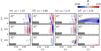
The most energetic spatial POD mode ( $\boldsymbol {\varPhi }^{(1)}$) is presented in figure 22 for representative planes, and the paired mode (
 $\boldsymbol {\varPhi }^{(2)}$) is not shown for brevity. The largest magnitudes of
 $\boldsymbol {\varPhi }^{(1)}$ occur in the aft portion of the LSB for
 $z/c\leq 2.15$, where shear layer vortices are observed in figure 17. A typical periodic spatial pattern of positive and negative wall-normal velocity seen in the aft portion of the field of view in figure 22(a–c) confirms the association between the dominant mode pair and the shear layer vortices within this spanwise region. The results show that the spanwise mode component is notably lower than the streamwise and wall-normal components at the onset of shear layer roll-up, supporting the earlier observation of nominally two-dimensional initial shear layer roll-up. However, an increase in the spanwise component of
 $\boldsymbol {\varPhi }^{(1)}$ can be seen at the same
 $x/c$ locations for
 $z/c=2.00$ and
 $2.15$, which is attributed to mixing between the fluid with greater negative spanwise velocity below the shear layer and the fluid with lesser negative spanwise velocity above the shear layer (figures 18b and 18c) induced by vortex shedding in the intermediate region. Although the r.m.s. spanwise velocity fluctuations associated with the breakdown of shear layer vortices are greater in the inboard region than in the intermediate region (figure 14c), coherent spanwise velocity fluctuations are not associated with the shear layer vortices in the inboard region because the difference in spanwise velocity between the fluid above and below the shear layer is much smaller (figure 18a). Mode
 $1$ at
 $z/c=2.25$ does not display a spatially periodic pattern associated with vortex formation, and modes
 $1$ and
 $2$ are no longer paired at this location, consistent with the absence of shear layer vortices in the tip region. Here, mode
 $1$ is mostly associated with the
 $u$-component fluctuations ascribed to shear layer flapping, which involves low frequency oscillations of the separated shear layer (Lengani et al. Reference Lengani, Simoni, Ubaldi, Zunino and Bertini2017b).
First spatial POD modes from side-view PIV. Masked flow area within  $0.21< x/c<0.30$ pertains to region of relatively high random errors near the wall.

The first four POD modes of  $(u',v')$ from the top-view measurements form two mode pairs that contain substantially higher modal energy content than higher modes (figure 20b). The chordwise component of the first (
 $\boldsymbol {\varPhi }^{(1)}$) and third (
 $\boldsymbol {\varPhi }^{(3)}$) spatial modes are presented in figure 23, with the paired modes
 $2$ and
 $3$ not shown for brevity. The results indicate that the first mode pair is associated with the shear layer vortices, with the characteristic streamwise wavelength matching that seen in the side-view mode projections of figure 22. In the inboard region, the spatial mode shapes of mode
 $1$ reflect strong two-dimensionality of the roll-up vortices. This is followed by progressive spanwise deformations for
 $Z/c>1.7$, with the shapes of the initial spanwise deformations following that of the mean reattachment line (dashed line). The contours of mode
 $3$ indicate that the second mode pair is associated with velocity fluctuations at twice the fundamental wavelength, i.e. at the subharmonic of the shedding frequency. The relative magnitude of the modal energy increases notably for
 $Z/c>2.00$, suggesting that the increased growth of the subharmonic mode is a result of wingtip effects. The amplification of disturbances at the subharmonic of the fundamental shear layer frequency has been associated with vortex merging in experiments on LSBs on two-dimensional airfoils (Yarusevych et al. Reference Yarusevych, Sullivan and Kawall2009; Kurelek, Yarusevych & Kotsonis Reference Kurelek, Yarusevych and Kotsonis2019). The merging of vortices in LSBs is often a localised phenomenon along the span, and has been speculated to be linked to cycle-to-cycle variations in the vortex strength or spacing in nominally two-dimensional LSBs (Kurelek et al. Reference Kurelek, Yarusevych and Kotsonis2019). This is consistent with the increased vortex deformations seen near the wingtip, which can promote localised vortex merging.
The  $u$ component of first and third top-view spatial POD modes of
 $(u',w')$. Dashed line: reattachment line from side-view stereo-PIV volumetric reconstruction.

For a statistical comparison of the wavelengths of shear layer disturbances in the LSB, the spatial power spectral density of the wall-normal component of velocity fluctuations ( $\mathcal {F}_{v'v'}$) was calculated for each instantaneous velocity field from the side-view configuration. The data were sampled along
 $y=\delta ^*_x$, over the streamwise extent of the field of view. The resulting spectra of streamwise wavelength (
 $\lambda$) were then averaged over all instantaneous velocity fields at each measurement plane, and the results are presented in figure 24. In figure 24(a), all spectra have been normalised by total energy and stepped by an order of magnitude to facilitate the identification of the dominant spectral peaks, while the comparison of the spectral energy content is facilitated by figure 24(b). In the inboard and intermediate regions
 $1.25\leq z/c\leq 2.25$, the results reveal clear spectral peaks within
 $0.037\leq \lambda /c \leq 0.043$, which are consistent with the spacing between vortices seen in figures 17 and 18. The associated spectral energy contours in figure 24(b) show maximum energy content reached inside the inboard and intermediate regions, while a notable decrease in the peak energy is seen at the boundaries of the intermediate region. The results also show a relative increase in the spectral energy of the subharmonic mode for
 $2.05\leq z/c \leq 2.25$, agreeing with the increase in the magnitude of the top-view subharmonic POD spatial mode (figure 23) at the outboard end of the intermediate region. However, the energy content associated with these fluctuations is relatively low, as can be seen in figure 24(b), and thus the overall impact on the LSB topology is not expected to be significant. As discussed earlier, the delayed and eventually suppressed separation and the associated reduction in the growth rates of disturbances delay transition near the wingtip, producing insignificant spectral content in the tip region in figure 24.
Streamwise wavelength spectra from side-view stereo-PIV at  $y=\delta ^*_x$. Dashed line:
 $\lambda /c=0.04$; dotted line:
 $\lambda /c=0.08$. Each spectrum in (a) is shifted by an order of magnitude at consecutive
 $z/c$ locations for clarity. (a) Normalised power spectral density and (b) power spectral density.

The spanwise variation of the fundamental wavelength ( $\lambda _0$) from the spectral analysis is presented in figure 25(a), along with the mean streamwise velocity at the mean location of maximum shape factor (
 $x=x_{H_{max}}$,
 $y=\delta ^*_x$) which approximates the average convective velocity of shear layer vortices (Boutilier & Yarusevych Reference Boutilier and Yarusevych2012b) at a given
 $z$ plane. The estimates are then used to obtain the shedding Strouhal number (
 $St_0=f_0c/U_\infty$, where
 $f_0\approx \bar {u}/\lambda _0$) which is presented in figure 25(b). The results confirm that the dominant streamwise wavelength of the vortices does not change appreciably across the span of the wing, despite notable changes to the mean bubble topology and vortex dynamics in the proximity of the wingtip. The associated shedding frequency shows minor variations across the span driven largely by the variations in the convective velocity estimates. The shedding frequency estimates agree to within the experimental uncertainty with the direct estimates from time-resolved measurements obtained by Toppings et al. (Reference Toppings, Kurelek and Yarusevych2021).
(a) Convection velocity at  $x=x_{H_{max}}$,
 $y=\delta ^*_x$ and fundamental wavelength. (b) Estimated fundamental vortex shedding frequency.

It is important to note that, based on measurements of two-dimensional LSBs on the same airfoil profile, a change in the effective angle of attack from approximately  $5^\circ$ at
 $z/c=1.25$ to
 $3^\circ$ at
 $z/c=2.15$ would result in a decrease in
 $St_0$ of approximately
 $20\,\%$ in a two-dimensional LSB (Boutilier & Yarusevych Reference Boutilier and Yarusevych2012a). In contrast, the variation of
 $St_0$ seen in figure 25 is non-monotonic and is confined primarily to within approximately
 $10\,\%$ of the inboard value largely due to experimental uncertainty. Thus, such spanwise uniformity in the mean LSB structure and transition process are surprising given the substantial change in the mean streamwise adverse pressure gradient along the span (figure 7b). Because the characteristics of the mean LSB and the dynamics of the transition process are interdependent, the relative spanwise uniformity of both the mean LSB topology and the transition statistics can be interpreted as an indication of the spanwise homogeneity of the transition process. Thus, it can be conjectured that shear layer transition within an LSB formed on a finite wing locks onto a common unstable mode across the span, with relatively small variations in the vortex dynamics compared with those expected due to the change in the effective angle of attack across the span.
4. Discussion
The results of this investigation demonstrate that significant changes to the LSB topology and dynamics take place in the relative proximity of the wingtip, eventually leading to open separation and effective termination of the LSB. Although no comparable three-dimensional velocity field measurements in LSBs are available on finite wings, a limited number of studies have conducted qualitative surface oil flow visualisations. It is of interest to explore the generality of the trends reported in § 3 across a wider parameter space, including other airfoil profiles, aspect ratios, Reynolds numbers and angles of attack, by comparing the trends observed in the LSB footprint on the wing suction surface. This is facilitated by table 2, which presents a summary of previous studies where LSB development on finite wings has been considered using surface flow visualisation and/or surface pressure measurements. The results of these studies suggest that the most predominant changes in the bubble footprint along the span are confined to a region of approximately one chord length from the wingtip across a range of different experimental conditions and geometries.
Comparison of selected previous studies involving LSBs on finite wings. Specified parameter ranges apply to pre-stall conditions where LSBs were explicitly detected in the corresponding studies. *Two unspecified pre-stall angles presented by the authors.

A more detailed comparison of the surface oil flow visualisation results from previous studies and the current results is facilitated in figures 26(a) and 26(b), which include data from investigations where mean separation and reattachment lines could be extracted without significant ambiguities. Figure 26 provides a comparison of separation and reattachment lines (figure 26a) and separation bubble length (figure 26b) at similar angles of attack. Because of the different aspect ratios employed, data are presented in terms of distance from the wingtip ( $z_{tip}-z$). It is important to note that the behaviour of separation and reattachment lines is extracted from surface visualisations and hence should be interpreted with caution near the wingtip. Specifically, the region of highly three-dimensional flow near the wingtip produces complex surface flow patterns that do not necessarily yield well-defined separation lines (e.g. figure 10b), making interpretation of oil flow visualisations difficult. Additionally, the wingtip vortex creates its own separation and reattachment lines (Giuni & Green Reference Giuni and Green2013), which may be difficult to distinguish from those attributable to the LSB. Nonetheless, similar to the present study, a consistent downstream shift in reattachment near the wingtip is observed in figure 26(a), and substantial changes in flow topology and separation bubble length are confined within approximately one chord length of the wingtip, in agreement with the general observations made in table 2. This suggests that the spanwise uniformity of the LSB away from the wingtip, revealed by the velocity field measurements of the present study in the inboard region, is a common feature of LSBs on finite wings under a variety of conditions. All identified separation lines extend closer to the wingtip than the corresponding reattachment lines, which is expected given the strengthening of the wingtip vortex with increasing
 $x/c$ (Francis & Katz Reference Francis and Katz1988). Further, while different trends are seen in the separation line estimates near the tip due to the aforementioned challenges in reliable separation identification, on the average, the results suggest a delayed reattachment and enlargement of the LSB. The three-dimensional velocity field measurements of the present study point to the reduction in shear layer vortex strength and delay in transition as the cause of the delayed reattachment observed near the wingtip in previous studies. Finally, termination of the reattachment lines in figure 26(a) prior to the wingtip points to the open nature of the LSBs in the tip region. Thus, the overall three-dimensional LSB structure revealed by the velocity field measurements of the present work is expected to persist on finite wings of various geometric and flow parameters for the aspect ratios sufficiently large to ensure that the flow across the entire wing is not comprised entirely by end-effect dominated regions (
 $AR\gtrsim 2$).
Separation line, reattachment line and bubble length comparison with selected previous studies. Solid and dashed lines in (a) are separation and reattachment lines, respectively. (b) Bubble length.

For a given airfoil profile, both the angle of attack and chord Reynolds number are known to influence the size and position of LSBs, with the former parameter associated with a more significant effect (Boutilier & Yarusevych Reference Boutilier and Yarusevych2012a). Since the strength of the wingtip vortex also shows a notable dependence on the angle of attack (Francis & Katz Reference Francis and Katz1988), changes in this parameter may be expected to lead to substantial changes in the extent of the region where LSB development is critically altered near the wingtip. To assess the spanwise extent of this region at varying angles of attack, figure 27 presents the distance between the wingtip ( $z_{tip}$) and the end of the LSB reattachment line (
 $z_{Rmax}$) extracted from the present and previous studies. The two studies with a NACA 0012 airfoil profile (Huang & Lin Reference Huang and Lin1995; Yen & Huang Reference Yen and Huang2009) suggest a decrease in the spanwise extent of the three-dimensional tip flow with increasing angle of attack. In contrast, on the average, the Wortmann profile used by Ananda et al. (Reference Ananda, Selig and Deters2018) and Bastedo & Mueller (Reference Bastedo and Mueller1986) displays an increase in the affected reattachment zone with increasing angle of attack. In addition to the aforementioned difficulties associated with the interpretation of the surface visualisations in the tip region, the observed discrepancy may be attributed to opposing effects of the angle of attack on the wingtip vortex and LSB. While an increase in the angle of attack increases the strength of the wingtip vortex and hence the spanwise extent of its effect on the suction side, it also moves the LSB upstream and reduces its length. Due to the decrease in the strength of the tip vortex towards the leading edge, the upstream movement of the LSB produces an opposing effect to the expected degree of spanwise influence. Consequently, since the LSB characteristics strongly depend on the profile shape, different and non-monotonic trends may be observed on different geometries, as seen in figure 27. However, for the variety of cases presented, the reattachment line ends no more than
 $0.6c$ from the wing tip, providing an approximate estimate of the maximum extent of the near-tip region where LSB suppression is expected to occur. Finally, a mild upstream movement of the reattachment point and shrinking of the LSB length with increasing chord Reynolds number, driven by the advancing transition, is expected to reduce the extent of the three-dimensional changes in LSBs on wings of a given geometry. This is reflected in the observations from Bastedo & Mueller (Reference Bastedo and Mueller1986), whose two data points in figure 27 show a reduction in
 $z_{tip}-z_{Rmax}$ from approximately
 $0.4c$ to
 $0.2c$ for
 $Re_c=8.0\times 10^4$ and
 $2.0\times 10^5$, respectively.
Distance between wingtip and estimated end of reattachment line. Experimental data on wings with the same airfoil profile are marked by the same symbol shapes.

5. Concluding remarks
The topology and dynamics of a LSB on a finite wing were investigated experimentally. A semispan wing and a reference two-dimensional airfoil configuration with a NACA 0018 airfoil profile were considered at a chord Reynolds number of  $1.25\times 10^5$ and an angle of attack of
 $6^\circ$, resulting in a typical short LSB on the suction surface. The flow development was explored using surface pressure measurements and PIV. Two configurations of PIV were employed to investigate the structure and dynamics of the three-dimensional LSB. The side-view, stereo-PIV configuration was used to obtain three-component velocity measurements in multiple planes along the span of the wing, while the top-view, two-component PIV measurements informed on the spanwise development of coherent structures forming in the aft portion of the bubble.
The results show that the LSB forming on a finite wing is largely two-dimensional in the inboard region where the spanwise pressure gradient is relatively low. In this region, spanwise variations in the streamwise extent and thickness of the separation bubble are relatively small, and the growth rates of disturbances in the separated shear layer are comparable to a two-dimensional airfoil at the same effective angle of attack. The LSB dynamics is dominated by shear layer vortices that are shed in the aft portion of the LSB. In the inboard region, the rollers form without appreciable spanwise deformations and are similar to those formed in LSBs on two-dimensional airfoils.
Near the wingtip, where the flow field is highly three-dimensional, the LSB becomes open and its topology differs substantially from that observed in the inboard region. A progressive reduction in boundary layer thickness occurs near the wingtip as a result of the downwash and reduction in adverse pressure gradient caused by the wingtip vortex. The reduction in separation bubble thickness near the wingtip stabilises the separated shear layer, which delays transition and shear layer roll-up. Within about  $0.2c$ from the wingtip, end effects are strong enough to prevent separation entirely.
Between the inboard region of the wing where the separation bubble is analogous to a separation bubble on a two-dimensional airfoil and the wingtip region where the separation bubble is terminated by three-dimensional end effects is an intermediate region where the separation bubble topology and dynamics are similar to those of the inboard region, but substantial spanwise variations in length, thickness, reverse flow velocity and vortex dynamics occur. Under the influence of significant spanwise flow, the thickness of the separation bubble increases, peaks and then reduces rapidly as the wingtip is approached. At the location of maximum separation bubble thickness, the most energetic roll-up vortices are observed, while closer to the wingtip, shear layer roll-up ceases entirely. Relative to the inboard region, progressively more pronounced spanwise deformations occur in the shear layer roll-up vortices in the intermediate region, and earlier vortex breakdown is observed, attributable to the destabilising effect of the spanwise momentum entrained into the vortex cores. This is also accompanied by a greater tendency for vortex merging. The stronger vortices forming here due to the local increase in the LSB height induce a local upstream advancement of the mean transition and reattachment locations. However, the spanwise changes in the mean locations of transition and reattachment are much smaller than those expected from the change in effective angle of attack along the span.
Despite the notable changes in LSB topology in the intermediate region and in the vicinity of the wingtip, the dominant streamwise wavelength and shedding frequency of the shear layer vortices remain largely invariant across the entire portion of the span where shedding is detected. The shedding persists to approximately within  $0.3c$ from the tip, and the LSB appears to lock onto a common instability mode across the span, despite the expected changes in the shear layer stability characteristics due to attendant changes of the effective angle of attack across the span. The substantial wingtip effects become progressively more significant starting from approximately
 $0.5c$ from the tip, and critical topological changes are confined to approximately
 $0.2c$ from the tip.
The comparative analysis of the present results with data extracted from surface flow visualisations detailed in a limited number of previous studies involving LSBs on wings shows that the time-average footprint of LSBs seen across a relatively wide parameter space is consistent with the main changes in mean bubble topology observed in the present study at moderate angles of attack. Thus, by extension, similar LSB topology and dynamics are expected on other wing geometries within a range of parameters where LSBs form on the inboard section of a wing. However, the results of the same analysis indicate that the extent of the characteristic flow regions observed in the present study is likely to change based on changes in flow and/or geometry parameters. Nonetheless, the available data suggest that relatively strong three-dimensional effects are expected to be confined to within one chord length from the wingtip and the open separation is not expected until approximately  $0.6c$ from the tip on wings with sufficiently large aspect ratios (
 $AR\gtrsim 2$).
Supplementary movies
Supplementary movies are available at https://doi.org/10.1017/jfm.2021.881.
Funding
The authors gratefully acknowledge the Natural Sciences and Engineering Research Council of Canada for funding this work.
Declaration of interest
The authors report no conflict of interest.