1 Introduction
Over the last three decades, flying insects have attracted great interest in the engineering and science fields because their length and velocity scales as well as the flight condition are similar to those of micro air vehicles (MAV) (Shyy et al. (Reference Shyy, Lian, Tang, Viieru and Liu2008, Reference Shyy, Aono, Kang and Liu2013); see also Pennycuick (Reference Pennycuick2008)). Typically MAV have a wing span of less than approximately 15 cm and mass of less than 100 g, and thus operate at low Reynolds numbers less than  $10^{5}$ (Spedding & Lissaman Reference Spedding and Lissaman1998; Ho et al. Reference Ho, Nassef, Pornsinsirirak, Tai and Ho2003; Shyy et al. Reference Shyy, Lian, Tang, Viieru and Liu2008, Reference Shyy, Aono, Kang and Liu2013). In this flow regime, the aerodynamic performance of a fixed wing such as the lift-to-drag ratio significantly deteriorates (Lissaman Reference Lissaman1983; Shyy et al. Reference Shyy, Lian, Tang, Viieru and Liu2008, Reference Shyy, Aono, Kang and Liu2013), while a flapping flight becomes more efficient due to the unsteady flow mechanisms (Spedding & Lissaman Reference Spedding and Lissaman1998; Ho et al. Reference Ho, Nassef, Pornsinsirirak, Tai and Ho2003; Shyy et al. Reference Shyy, Lian, Tang, Viieru and Liu2008, Reference Shyy, Aono, Kang and Liu2013). Therefore, the mechanisms of lift generation due to flapping flight of various flying insects such as the fruit fly, bumblebee, hawkmoth, rhinoceros beetle, cicada and mosquito have been investigated by numerous researchers (Dudley & Ellington Reference Dudley and Ellington1990; Willmott, Ellington & Thomas Reference Willmott, Ellington and Thomas1997; Dickinson, Lehmann & Sane Reference Dickinson, Lehmann and Sane1999; Le et al. Reference Le, Truong, Park, Truong, Ko, Park and Byun2013; Zheng, Hedrick & Mittal Reference Zheng, Hedrick and Mittal2013; Liu, Dong & Li Reference Liu, Dong and Li2016; Bomphrey et al. Reference Bomphrey, Nakata, Phillips and Walker2017).
In this study, we focus on a rhinoceros beetle, Trypoxylus dichotomus, among various flying insects, because it is one of the heaviest insects and has the highest wing loading among the biological flyers that satisfy the weight and size requirements of MAV: e.g. the mass and wing loading are around 0.72 mg and  $2.6~\text{N}~\text{m}^{-2}$ for a fruit fly, 0.175 g and
 $16.2~\text{N}~\text{m}^{-2}$ for a bumblebee (Sun & Du Reference Sun and Du2003), 1.39 g and
 $7.8~\text{N}~\text{m}^{-2}$ for a hawkmoth (Zheng et al. Reference Zheng, Hedrick and Mittal2013), 1.18 g and
 $11.8~\text{N}~\text{m}^{-2}$ for a cicada (Wan, Dong & Gai Reference Wan, Dong and Gai2015), and 6 g and
 $38~\text{N}~\text{m}^{-2}$ for a rhinoceros beetle (Lee, Park & Kim Reference Lee, Park and Kim2015a). Since high wing loading allows a flyer to carry a larger payload and a higher capacity of fuel, it can increase the range and economy of the mission of the MAV (Ho et al. Reference Ho, Nassef, Pornsinsirirak, Tai and Ho2003). However, a flyer having high wing loading may require high weight-specific power or have low agility and manoeuvrability. Therefore, when designing a beetle-like flapping-wing micro air vehicle with high wing loading, optimizing the wing kinematics and geometry is necessary to reduce the energy cost of the flight or to improve the aerodynamic performance while generating sufficiently high wing loading.
For the purpose of optimizing the kinematics and geometry of a flapping wing, a predictive tool, which accurately predicts the aerodynamic performance, is required for a systematic design. Thus, a few aerodynamic models have been developed to predict the aerodynamic characteristics of flapping wings. According to Ansari, Zbikowski & Knowles (Reference Ansari, Zbikowski and Knowles2006a), aerodynamic models for flapping flight can be distinguished by three different approaches: steady-state, unsteady and quasi-steady approaches. Steady-state approaches include actuator disk momentum theory (Ellington Reference Ellington1984b) and steady vortex theory (Rayner Reference Rayner1979), and provide information about the time-averaged downwash motion induced by vortical structures around a flapping wing once a periodic state is reached. However, their applicability is limited when unsteady aerodynamic performance is required. On the other hand, unsteady approaches based on the potential flow conditions consider the effects of the leading and trailing edge vortices by applying Kutta-like boundary conditions at both edges (for examples see, Ansari, Zbikowski & Knowles (Reference Ansari, Zbikowski and Knowles2006b); Xia & Mohseni (Reference Xia and Mohseni2013)). As noted in Ansari et al. (Reference Ansari, Zbikowski and Knowles2006a), however, the applicability of these boundary conditions is questionable during stroke reversal, because wing pitching motion is so acute that the fluid is more likely to turn around the trailing edge rather than leaving the edge smoothly. Quasi-steady approaches assume that each instantaneous aerodynamic characteristic of flapping wings is taken to be the steady-state solution obtained by fixing the corresponding wing motion in time. However, to improve their prediction performance, most of the existing quasi-steady approaches contain model constants that should be provided a priori by experiments or numerical simulations whenever the wing geometry changes (Sane & Dickinson Reference Sane and Dickinson2002; Berman & Wang Reference Berman and Wang2007; Whitney & Wood Reference Whitney and Wood2010; Nakata, Liu & Bomphrey Reference Nakata, Liu and Bomphrey2015). For this reason, optimizations based on quasi-steady approaches have been limited only for the wing kinematics (Berman & Wang Reference Berman and Wang2007; Zheng et al. Reference Zheng, Hedrick and Mittal2013; Nakata et al. Reference Nakata, Liu and Bomphrey2015). Recently, Wang, Goosen & van Keulen (Reference Wang, Goosen and van Keulen2016) suggested a predictive aerodynamic model for flapping flight without any model constants by providing them based on theoretical approaches and observations. Nonetheless, their model has a limitation in that it neglects the effects of the fluid viscosity and wing–wake interaction.
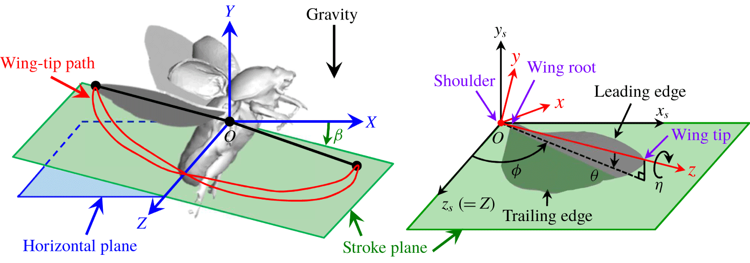
Wing kinematic parameters and coordinates.

Hovering flight in general requires more power than other flight modes because there is no ambient wind to aid in lift generation (Berman & Wang Reference Berman and Wang2007). Also, flapping wings in hovering flight interact with their own wake generated by the previous strokes (Birch & Dickinson Reference Birch and Dickinson2003; Aono, Liang & Liu Reference Aono, Liang and Liu2008), which should be considered in developing a quasi-steady aerodynamic model. So far, the aerodynamic performance of the hovering flight of various species of insects such as the fruit fly, bumblebee and hawkmoth has been extensively studied (Dickinson et al. Reference Dickinson, Lehmann and Sane1999; Wang, Birch & Dickinson Reference Wang, Birch and Dickinson2004; Berman & Wang Reference Berman and Wang2007; Aono et al. Reference Aono, Liang and Liu2008; Zheng et al. Reference Zheng, Hedrick and Mittal2013; Nakata et al. Reference Nakata, Liu and Bomphrey2015). However, the hovering flight of a rhinoceros beetle (Truong et al. Reference Truong, Phan, Park and Ko2013a, Reference Truong, Le, Park and Byun2017; Phan, Truong & Park Reference Phan, Truong and Park2017) has not received much attention compared to other flying insects, and further investigations are needed for understanding its aerodynamic mechanism. Therefore, the objectives of our study are (i) to investigate the aerodynamic characteristics of a hovering flight of a rhinoceros beetle using numerical simulations and (ii) to suggest an improved predictive aerodynamic model of flapping flight in hover without any ad hoc model constants. We also examine the aerodynamic role of the elytron (fore wing) and body and the effect of a twisted hind wing along the wing span. In § 2, we provide the wing kinematics of a rhinoceros beetle in a hovering flight. The numerical details and results are given in §§ 3 and 4. In § 5, we suggest an improved predictive aerodynamic model of a flapping wing in hover, based on the previous model of Wang et al. (Reference Wang, Goosen and van Keulen2016), by combining a quasi-steady blade element theory with a momentum theory to include the effect of the wing–wake interaction. This predictive model is validated by comparing the results with those from numerical simulation in §§ 6 and 7, followed by conclusions in § 8.
2 Wing kinematics and morphological parameters
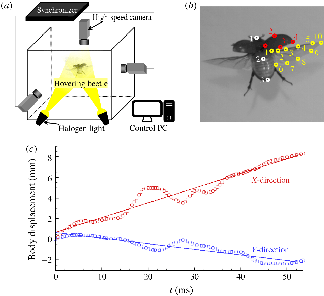
Wing motions of a hovering rhinoceros beetle (Trypoxylus dichotomus) are measured using high-speed cameras (experimental details are given in appendix A), and their kinematics are averaged over two flapping periods. Figure 1 shows the wing kinematic parameters and coordinates, which are defined in a conventional way as is done in Willmott & Ellington (Reference Willmott and Ellington1997), Fry, Sayaman & Dickinson (Reference Fry, Sayaman and Dickinson2005), Aono et al. (Reference Aono, Liang and Liu2008), and Zheng et al. (Reference Zheng, Hedrick and Mittal2013). The  $(X,Y,Z)$ coordinate is fixed at the shoulder of the right hind wing. The
 $(X,Z)$ plane is the horizontal plane perpendicular to the gravity direction, and the
 $Y$-axis is opposite to the gravity direction. The
 $X$-axis is the forward direction and the
 $Z$-axis is the right lateral direction. The stroke plane angle (
 $\unicode[STIX]{x1D6FD}$) is defined as the angle between the horizontal
 $(X,Z)$ and stroke planes, where the latter is the plane connecting the locations of the shoulder and wing tip at the ends of the downstroke and upstroke. The
 $(x_{s},y_{s},z_{s})$ coordinate is defined such that
 $y_{s}$ is the direction normal to the stroke plane,
 $z_{s}=Z$, and
 $x_{s}$ is in compliance with the right-hand rule. This coordinate is transformed to the
 $(x,y,z)$ coordinate co-rotating with the wing by three consecutive rotations (sweeping, out-of-plane deviation, and pitching motions), where
 $x$,
 $y$ and
 $z$ axes indicate the wing thickness-wise, chordwise, and spanwise directions, respectively. Here, the sweeping angle (
 $\unicode[STIX]{x1D719}$) is defined as the angle between the
 $z_{s}$-axis and the projection of the
 $z$-axis on the stroke plane. The angle between the stroke plane and the
 $z$-axis is defined as the out-of-plane deviation angle (
 $\unicode[STIX]{x1D703}$). Finally, the pitching angle (
 $\unicode[STIX]{x1D702}$) is the angle of rotation about the
 $z$-axis.
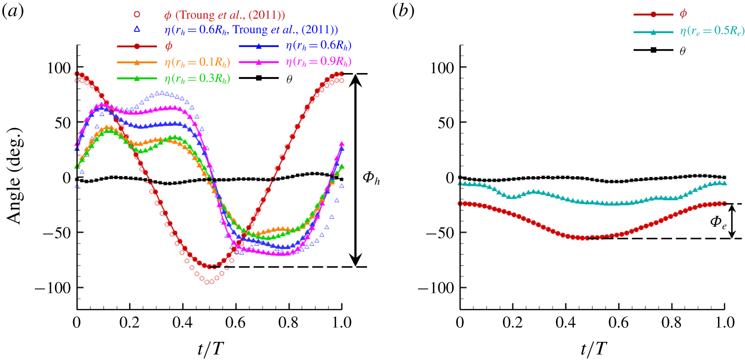
Wing kinematics measured: (a) hind wing; (b) elytron. In (a), sweeping and pitching angles of a hind wing measured by Truong et al. (Reference Truong, Nguyen, Truong, Park, Byun and Goo2011) are also plotted.

Figure 2 shows the measured wing kinematics of the right hind wing and elytron (see supplementary materials available at https://doi.org/10.1017/jfm.2019.962). To obtain smooth changes in the angular accelerations, all angles in time are connected using periodic quintic splines (Schurer Reference Schurer1968). The flapping frequencies for both wings are  $f(=1/T)=37.04~\text{Hz}$, and the body inclination angle is
 $85.9^{\circ }$ with respect to the horizontal plane
 $(X,Z)$. The stroke plane angles for the hind wing and elytron are
 $\unicode[STIX]{x1D6FD}_{h}=2.25^{\circ }$ and
 $\unicode[STIX]{x1D6FD}_{e}=10.15^{\circ }$, where the subscripts of
 $h$ and
 $e$ denote the hind wing and elytron, respectively. The elytron moves in phase with the hind wing, but the sweeping amplitude of the hind wing (
 $\unicode[STIX]{x1D6F7}_{h}=175^{\circ }$) is approximately 5.6 times that of the elytron (
 $\unicode[STIX]{x1D6F7}_{e}=31.3^{\circ }$). It is observed that both wings become closest to each other at
 $t/T\approx 0.37$ and
 $0.63$, where
 $t/T=0$ corresponds to the start of the upstroke. Also, the sweeping motions of both wings are almost simple harmonic. Therefore, the durations of both the upstroke (
 $0\leqslant t/T\lesssim 0.5$) and downstroke (
 $0.5\lesssim t/T\leqslant 1$) are nearly identical. Since the hind wing is highly flexible but the elytron is almost rigid, the pitching angles of the hind wing at four different spanwise positions (
 $r_{h}/R_{h}=0.1,0.3,0.6$ and 0.9) are measured, but that of the elytron is measured only at the midspan (
 $r_{e}/R_{e}=0.5$), where
 $r$ and
 $R$ are the spanwise distance from the wing root (see figure 3) and the wing length (root to tip), respectively. The pitching motion of the hind wing is qualitatively similar to those of other insect wings measured by previous studies (Jensen Reference Jensen1956; Vogel Reference Vogel1967; Ellington Reference Ellington1984a). Although there are some humps in the pitching angles that may be associated with passive pitching motion due to the air–wing interaction, the pitching angle at each spanwise position remains roughly constant during most of the half-stroke but rapidly changes near the start and end of the half-stroke. At the end of upstroke (
 $t/T\approx 0.5$),
 $\unicode[STIX]{x1D702}\approx 0^{\circ }$ (indicating a symmetric rotation), whereas
 $\unicode[STIX]{x1D702}$ is already positive at the end of downstroke (
 $t/T=1$) (indicating an advanced rotation) (Dickinson et al. Reference Dickinson, Lehmann and Sane1999). Also, the pitching amplitude near the wing tip is much larger than that near the wing root, indicating that the hind wing is significantly twisted during the stroke. When we define the amount of wing twist as the difference in the pitching angles at
 $r_{h}/R_{h}=0.1$ and 0.9, the amounts of the hind wing twist are approximately
 $25^{\circ }$ and
 $15^{\circ }$ during most of the upstroke and downstroke, respectively. A similar amount of wing twist (
 $10^{\circ }\sim 20^{\circ }$) was found for some other insects (Ellington Reference Ellington1984a). On the other hand, the pitching amplitude of the elytron is much smaller than that of the hind wing and remains nearly constant (
 $\unicode[STIX]{x1D702}\approx -15^{\circ }$) throughout the full stroke. For both wings, the out-of-plane motions are negligible (
 $\unicode[STIX]{x1D703}\approx 0^{\circ }$).
For comparison, the sweeping and pitching (at  $r_{h}/R_{h}=0.6$) angles of a hind wing measured by Truong et al. (Reference Truong, Nguyen, Truong, Park, Byun and Goo2011) are also provided in figure 2(a). In their study, the measured flapping frequency was approximately 37.7 Hz, which is almost the same as that of the present study (
 $f=37.04~\text{Hz}$). The present sweeping motion (
 $\unicode[STIX]{x1D719}$) of the hind wing is in excellent agreement with that of Truong et al. (Reference Truong, Nguyen, Truong, Park, Byun and Goo2011), and the present pitching angle (
 $\unicode[STIX]{x1D702}$) reasonably agrees with that of Truong et al. (Reference Truong, Nguyen, Truong, Park, Byun and Goo2011). Note, however, that the present stroke plane angle of the hind wing (
 $\unicode[STIX]{x1D6FD}_{h}\approx 2.25^{\circ }$) is quite different from that (
 $\unicode[STIX]{x1D6FD}_{h}\approx 30^{\circ }$) of Truong et al. (Reference Truong, Nguyen, Truong, Park, Byun and Goo2011). This might be caused by the difference between the body inclination angle of the present study and that of Truong et al. (Reference Truong, Nguyen, Truong, Park, Byun and Goo2011).
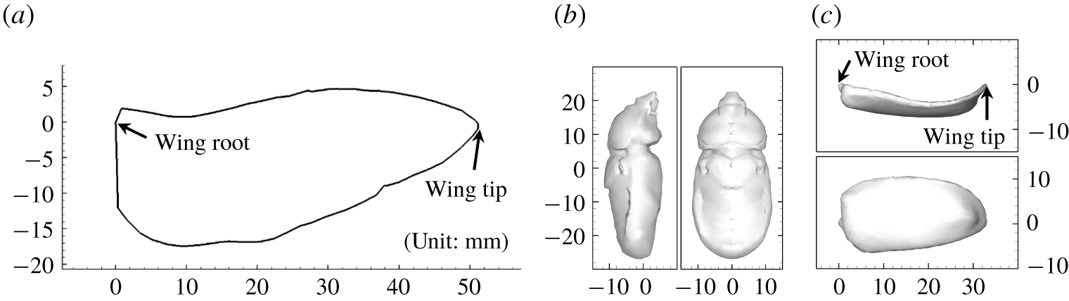
Wing and body geometries: (a) hind wing (planform view); (b) body; (c) elytron. Here, the legs are removed from the scanned body.

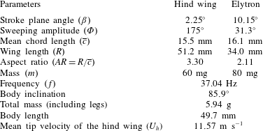
Measured kinematic and morphological parameters.

To measure the morphological parameters of the beetle whose wing kinematics are recorded, the hind wing and elytron are detached from the body. The body and elytron are three-dimensionally scanned, but only the planform geometry is measured for the hind wing (see figure 3 and supplementary materials). Table 1 summarizes the measured morphological and kinematic parameters. The mean chord lengths, wing lengths, aspect ratios, and mass of the hind wing and elytron are  $\overline{c}_{h}=15.5~\text{mm}$ and
 $\overline{c}_{e}=16.1~\text{mm}$,
 $R_{h}=51.2~\text{mm}$ and
 $R_{e}=34.0~\text{mm}$,
 $AR_{h}=3.30$ and
 $AR_{e}=2.11$, and
 $m_{h}=60~\text{mg}$ and
 $m_{e}=80~\text{mg}$, respectively, where
 $AR=R/\overline{c}$. The total mass (including legs) and body length are
 $m=5.94$ g and
 $l_{b}=49.7~\text{mm}$. The Reynolds number is
 $Re=U_{h}\overline{c}_{h}/\unicode[STIX]{x1D708}=12\,000$, where
 $U_{h}(=2\unicode[STIX]{x1D6F7}_{h}\,fR_{h})$ is the time-averaged velocity of the hind wing at the tip and
 $\unicode[STIX]{x1D708}$ is the kinematic viscosity of air.
3 Numerical method
For conducting the numerical simulations, we use the measured wing kinematics and wing and body geometries shown in figures 2 and 3. We use an immersed boundary method in an inertial reference frame (Kim, Kim & Choi Reference Kim, Kim and Choi2001) to satisfy no-slip on the body and wing surfaces. The governing equations for unsteady three-dimensional incompressible viscous flow are
 $$\begin{eqnarray}\displaystyle & \displaystyle \unicode[STIX]{x1D735}\boldsymbol{\cdot }\boldsymbol{u}-q=0, & \displaystyle\end{eqnarray}$$
 $$\begin{eqnarray}\displaystyle & \displaystyle \frac{\unicode[STIX]{x2202}\boldsymbol{u}}{\unicode[STIX]{x2202}t}+\unicode[STIX]{x1D735}\boldsymbol{\cdot }(\boldsymbol{u}\boldsymbol{u})=-\unicode[STIX]{x1D735}p+\frac{1}{Re}\unicode[STIX]{x1D6FB}^{2}\boldsymbol{u}+\boldsymbol{f}, & \displaystyle\end{eqnarray}$$
where  $\boldsymbol{u}$ is the flow velocity,
 $p$ is the pressure, and
 $q$ and
 $\boldsymbol{f}$ are, respectively, the mass source/sink and momentum forcing used for the immersed boundary method (see Kim et al. Reference Kim, Kim and Choi2001 for the detail). A second-order semi-implicit time advancement scheme (a third-order Runge–Kutta method for the convection terms and the Crank–Nicolson method for the viscous terms) is used for time integration, and the second-order central difference is used for all spatial derivatives. The computations are performed at the maximum CFL (Courant–Friedrichs–Lewy) number of 1. All variables are non-dimensionalized by
 $U_{h}$ and
 $\overline{c}_{h}$.
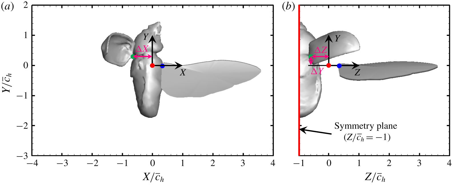
Body configuration: (a) side and (b) rear views of a hovering rhinoceros beetle having the body inclination of  $85.9^{\circ }$ with respect to the horizontal plane (
 $X{-}Z$ plane). The symmetry plane (
 $Z/\overline{c}_{h}=-1$) locates at the centre of the body. The distance between shoulders of hind wing and elytron (denoted as red and green solid circles, respectively) is
 $\unicode[STIX]{x0394}X=0.65\overline{c}_{h}$,
 $\unicode[STIX]{x0394}Y=0.3\overline{c}_{h}$ and
 $\unicode[STIX]{x0394}Z=0.6\overline{c}_{h}$. Note that the shoulder and root locations of the elytron are identical, but those (red and blue solid circles, respectively) of the hind wing are separated by
 $0.3\overline{c}_{h}$ (see also § 4).

Fine grid region. For each grid system, the smallest grids  $\unicode[STIX]{x1D6E5}_{min}(=\unicode[STIX]{x0394}X_{min}=\unicode[STIX]{x0394}Y_{min}=\unicode[STIX]{x0394}Z_{min})$ are uniformly located at the fine grid region and stretched grids are used elsewhere. Sizes of grid and domain are non-dimensionalized by the mean chord length of the hind wing (
 $\overline{c}_{h}$).

The size of the computational domain is  $-25<X/\overline{c}_{h}<25$,
 $-30<Y/\overline{c}_{h}<20$ and
 $-1<Z/\overline{c}_{h}<30$, where
 $Z/\overline{c}_{h}=-1$ corresponds to the symmetry plane at the body centre (see figure 4). We apply the Dirichlet boundary condition of
 $\boldsymbol{u}=0$ at the outer boundary surfaces and the symmetry boundary condition of
 $\unicode[STIX]{x2202}U/\unicode[STIX]{x2202}Z=0$,
 $\unicode[STIX]{x2202}V/\unicode[STIX]{x2202}Z=0$ and
 $W=0$ at
 $Z/\overline{c}_{h}=-1$, where
 $U$,
 $V$ and
 $W$ are the velocity components in the
 $X$,
 $Y$ and
 $Z$ directions, respectively. Table 2 summarizes the details of the grid resolutions and the total number of grids for grid dependence tests. To resolve the flow around the hind wing surfaces, the smallest grids
 $\unicode[STIX]{x1D6E5}_{min}(=\unicode[STIX]{x0394}X_{min}=\unicode[STIX]{x0394}Y_{min}=\unicode[STIX]{x0394}Z_{min})$ are uniformly located at
 $-3.8<X/\overline{c}_{h}<3.8$,
 $-2.8<Y/\overline{c}_{h}<1.6$ and
 $-1<Z/\overline{c}_{h}<3.8$ for grids I and II, but at
 $-4<X/\overline{c}_{h}<4$,
 $-3<Y/\overline{c}_{h}<2$ and
 $-1<Z/\overline{c}_{h}<4$ for grid III, respectively, and stretched grids are used elsewhere:
 $449(X)\times 289(Y)\times 289(Z)$ with
 $\unicode[STIX]{x1D6E5}_{min}=0.02\overline{c}_{h}$ (grid I),
 $897\times 577\times 577$ with
 $\unicode[STIX]{x1D6E5}_{min}=0.01\overline{c}_{h}$ (grid II), and
 $545\times 381\times 321$ with
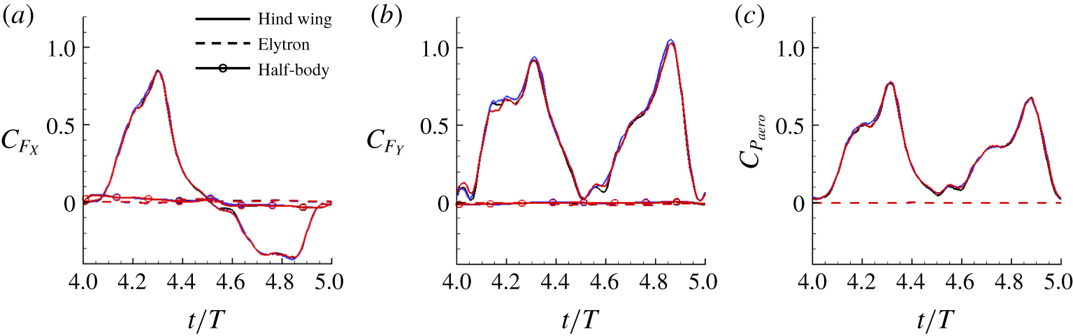
 $\unicode[STIX]{x1D6E5}_{min}=0.02\overline{c}_{h}$ (grid III), respectively. For all grids, the flows reach quasi-periodic states after four periods. Figure 5 shows the horizontal and vertical force and aerodynamic power coefficients from three different grids, where
 $C_{F_{i}}=2F_{i}/\unicode[STIX]{x1D70C}U_{h}^{2}R_{h}\overline{c}_{h}$,
 $C_{P_{aero}}=2P_{aero}/\unicode[STIX]{x1D70C}U_{h}^{3}R_{h}\overline{c}_{h}$,
 $F_{X}$ and
 $F_{Y}$ are the horizontal and vertical forces,
 $P_{aero}$ is the aerodynamic power and
 $\unicode[STIX]{x1D70C}$ is the density of air. These aerodynamic forces and power are evaluated by the method of Lee et al. (Reference Lee, Kim, Choi and Yang2011), and are given by
 $$\begin{eqnarray}\displaystyle & \displaystyle \frac{\boldsymbol{F}}{\unicode[STIX]{x1D70C}U_{h}^{2}\overline{c}_{h}^{2}}=\int _{V_{w}}\left[-\boldsymbol{f}+\frac{\unicode[STIX]{x2202}\boldsymbol{u}}{\unicode[STIX]{x2202}t}+\unicode[STIX]{x1D735}\boldsymbol{\cdot }(\boldsymbol{u}\boldsymbol{u})\right]\,\text{d}V, & \displaystyle\end{eqnarray}$$
 $$\begin{eqnarray}\displaystyle & \displaystyle \frac{P_{aero}}{\unicode[STIX]{x1D70C}U_{h}^{3}\overline{c}_{h}^{2}}=-\int _{V_{w}}\boldsymbol{v}\boldsymbol{\cdot }\left[-\boldsymbol{f}+\frac{\unicode[STIX]{x2202}\boldsymbol{u}}{\unicode[STIX]{x2202}t}+\unicode[STIX]{x1D735}\boldsymbol{\cdot }(\boldsymbol{u}\boldsymbol{u})\right]\,\text{d}V, & \displaystyle\end{eqnarray}$$
where  $\boldsymbol{v}$ and
 $V_{w}$ are the wing velocity and control volume enclosing each isolated wing or body, respectively. As shown in figure 5, the results from grids I, II and III are nearly identical, and their differences in the period-averaged horizontal and vertical forces and aerodynamic power from grids I and II are less than 2 %. Since grid III has
 $\unicode[STIX]{x1D6E5}_{min}$ on a slightly wider area than grids I and II, we hereafter provide results from grid III.
Results of grid dependence tests for case 3 (see § 4): (a) horizontal force coefficient; (b) vertical force coefficient; (c) aerodynamic power coefficient. Blue, black and red lines denote the results from grids I, II and III, respectively.

The cross-section of the hind wing at each spanwise location is modelled as a rigid and flat plate with a rectangular shape having a thickness of 0.06 $\overline{c}_{h}$ assuming that the aerodynamic effect of wing corrugation is small in hovering flight (Meng, Xu & Sun Reference Meng, Xu and Sun2011). Although the hind wing thickness considered is thicker than that of a rhinoceros beetle (the maximum thickness of the vein at the wing base and the average thickness of the membrane of a rhinoceros beetle were measured to be approximately
 $715~\unicode[STIX]{x03BC}\text{m}$ (0.05
 $\overline{c}_{h}$) and
 $3.57~\unicode[STIX]{x03BC}\text{m}$ (0.0002
 $\overline{c}_{h}$), respectively (Jin et al. Reference Jin, Goo, Woo and Park2009)), a similar wing thickness has been used to investigate the aerodynamic performance of the flapping wings in many previous studies (Sun & Tang Reference Sun and Tang2002; Kweon & Choi Reference Kweon and Choi2010; Truong et al. Reference Truong, Kim, Kim, Park, Yoon and Byun2013b). We conduct two additional simulations for case 1 (flat hind wing only) with the wing thickness of 0.02
 $\overline{c}_{h}$ and 0.04
 $\overline{c}_{h}$, respectively. The results indicate that the effects of the wing thickness on the force and power are negligible at least for the range of the wing thickness considered.
4 Simulation results
In this section, we examine the aerodynamic roles of the body, elytron and twisted hind wing using numerical simulation. We simulate six different cases (see also table 3) for rigid flat and twisted hind wings: hind wing only (cases 1 and 4), hind wing and elytron (cases 2 and 5), and hind wing, elytron and half-body (cases 3 and 6), respectively. For the twisted hind wing, the pitching angles are measured at  $r_{h}/R_{h}=0.1,0.3,0.6$ and 0.9, and they are connected using cubic splines for the whole wing span. For the flat hind wing, the pitching angle is constant along the spanwise direction, and its value is taken to be the same as that at
 $r_{h}/R_{h}$=0.6. For the rigid flat hind wings (cases 1–3), the pitching motion is less realistic, and thus a collision occurs between the body and the trailing edge near the root of the hind wing. To avoid this problem, the root of the hind wing is slightly offset by 0.3
 $\overline{c}_{h}$ from the shoulder (see figure 4). This offset is also applied to the cases of the twisted wing (cases 4–6). Due to this offset, the tip velocity of the hind wing increases by the factor of
 $(R_{h}+0.3\overline{c}_{h})/R_{h}$. To keep the wing tip velocity (and thus the Reynolds number) unchanged, the flapping frequency is slightly reduced such that
 $f^{\prime }=fR_{h}/(R_{h}+0.3\overline{c}_{h})$. Since
 $R_{h}=3.3\overline{c}_{h}$, the frequency is reduced by approximately 8.3 %. To see how much the aerodynamic forces are changed due to this offset, we compare the results for case 1 with and without the offset. It turns out that the forces are changed by approximately 10 % due to the offset. We also neglect the out-of-plane motions of the hind wing and elytron (i.e.
 $\unicode[STIX]{x1D703}=0^{\circ }$) because they are insignificant, as shown in figure 2. One may also wonder if the starting position of a flapping wing affects the aerodynamic performances. To answer this question, we perform an additional simulation starting from the downstroke (as opposed to starting from the upstroke) for case 3. We find that the aerodynamic performances are changed for the first few cycles by a different starting position, but those changes almost disappear in the quasi-periodic state (e.g. at
 $t/T\geqslant 4$).
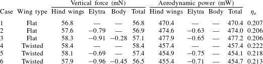
Mean vertical force and aerodynamic power averaged over the fifth cycle ( $4\leqslant t/T<5$), and hovering efficiency
 $(\unicode[STIX]{x1D702}_{a}=\overline{C}_{F_{Y}}^{3/2}/(\sqrt{2\unicode[STIX]{x1D6F7}_{h}AR_{h}\cos \unicode[STIX]{x1D6FD}_{h}}\,\overline{C}_{P_{aero}}))$.

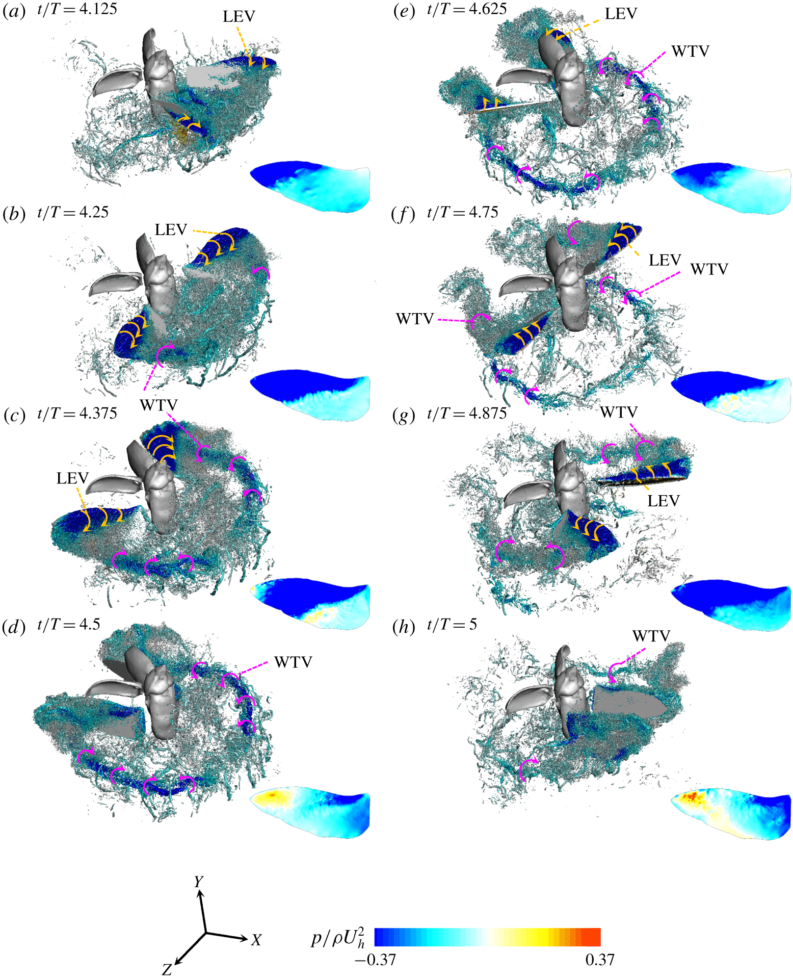
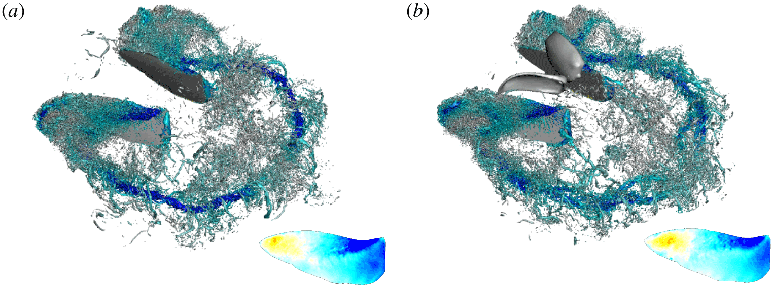
Development of vortical structures, identified by the iso-surface of  $\unicode[STIX]{x1D706}_{2}=-12.34$ (Jeong & Hussain Reference Jeong and Hussain1995), during the fifth period (flat hind wing; case 3), coloured by the contours of the instantaneous pressure. The instantaneous pressure on the suction surface of the hind wing are obtained by the interpolation method of Kim, Lee & Choi (Reference Kim, Lee and Choi2018) and its contours are also plotted in this figure. Note that the simulations are conducted with the right half of the body and wings. So, the flow fields in the left half in this figure are obtained by mirroring the results in the right half.

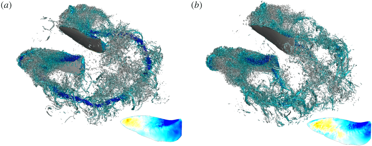
Effects of the presence of the elytron and body on the vortical structures and pressure around the hind wing at  $t/T=4.5$: (a) hind wing only (case 1); (b) hind wing and elytron (case 2). The contours of the instantaneous pressure on the suction surface of the hind wing are also plotted in this figure. The
 $\unicode[STIX]{x1D706}_{2}$ isosurfaces and colour contours are the same as those in figure 6. Also, the vortical structures in the left half of the body and wings are from those in the right half as done in figure 6.

As shown in figure 5, it is clear that the force and power from the elytron and body are negligible and they almost come from the hind wing. Figure 6 shows the instantaneous vortical structures around a hovering rhinoceros beetle model with the rigid flat hind wing (case 3) during the fifth period, together with the contours of the pressure on the suction surface and around the hind wing. At  $t/T=4.125$, the hind wing accelerates backward and a leading edge vortex (LEV) is generated at the suction surface near the hind wing tip where a low pressure region exists (figure 6a). As time goes by, a wing tip vortex (WTV) is also generated along the hind wing tip path (figures 6b and 6c). At
 $t/T=4.25$, the LEV grows but remains attached on the suction surface of the hind wing, and thus the low pressure region becomes wider (figure 6b). During the wing deceleration (
 $t/T=4.375$), the LEV begins to be shed from the suction surface very near the hind wing tip (figure 6c). At the end of the upstroke (
 $t/T=4.5$), the LEV on the hind wing is entirely shed from the suction surface near the tip, and this region changes to a high pressure region due to the motion induced by a detached LEV (figure 6d). Also, an arc-like WTV generates a downwash motion in the wake. Similar vortical structures (LEV and WTV) and pressure fields are observed around the hind wing during the downstroke (figure 6e–h). On the other hand, the sizes and strengths of vortical structures around the elytron and body are much smaller than those around the hind wing. Accordingly, as shown in figure 7, the vortical structures around the hind wing and the pressure field are not significantly affected by the presence of the elytron and body. Therefore, the horizontal and vertical force and aerodynamic power coefficients obtained for cases 1 and 2 are nearly the same as those for case 3 (figure 5), indicating that the elytron and body generate negligible aerodynamic forces and require little aerodynamic power compared to those for the hind wing during the hovering flight.
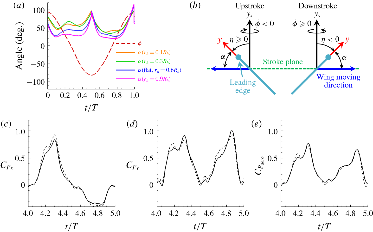
As shown in figure 2, the hind wing is twisted and thus the angle of attack varies along the span during flapping. Since we consider  $\unicode[STIX]{x1D703}=0^{\circ }$,
 $\unicode[STIX]{x1D6FC}=\unicode[STIX]{x03C0}/2+\text{sgn}(\dot{\unicode[STIX]{x1D719}})\unicode[STIX]{x1D702}$, where
 $\dot{\unicode[STIX]{x1D719}}=\text{d}\unicode[STIX]{x1D719}/\text{d}t$,
 $\text{sgn}(\bullet )$ is the signum function (1 and
 $-1$ for real positive and negative numbers, respectively, and 0 for zero) (see figure 8(a,b)). In figure 8(c–e), we compare the horizontal and vertical force, and aerodynamic power coefficients, of the rigid twisted hind wing with those of the flat one. Here, we consider hind wings only (cases 1 and 4), because the aerodynamic roles of the elytron and the body are negligible. The force and power coefficients of the twisted hind wing are slightly increased and decreased, respectively, as compared to those of the flat wing. Figure 9 shows the instantaneous vortical structures and pressure around the flat and twisted hind wings at
 $t/T=4.5$. As observed in figure 8(a), the angle of attack of the twisted wing is large near the wing root but smaller near the tip compared to that of the flat wing. Therefore, the tip vortices are much stronger for the flat wing than those for the twisted wing, whereas the root vortices are stronger for the twisted wing. At this instant (
 $t/T=4.5$), however, the angles of attack of the twisted wing are not very different from that of the flat one (see figure 8a), and thus the difference in the surface pressures of the flat and twisted wings is not large. We further investigate the effect of the wing twist on the time-averaged sectional lift (
 $\unicode[STIX]{x0394}\overline{L}$), drag (
 $\unicode[STIX]{x0394}\overline{D}$) and power (
 $\unicode[STIX]{x0394}\overline{P}_{aero}$). Here, the directions of lift and drag are perpendicular (
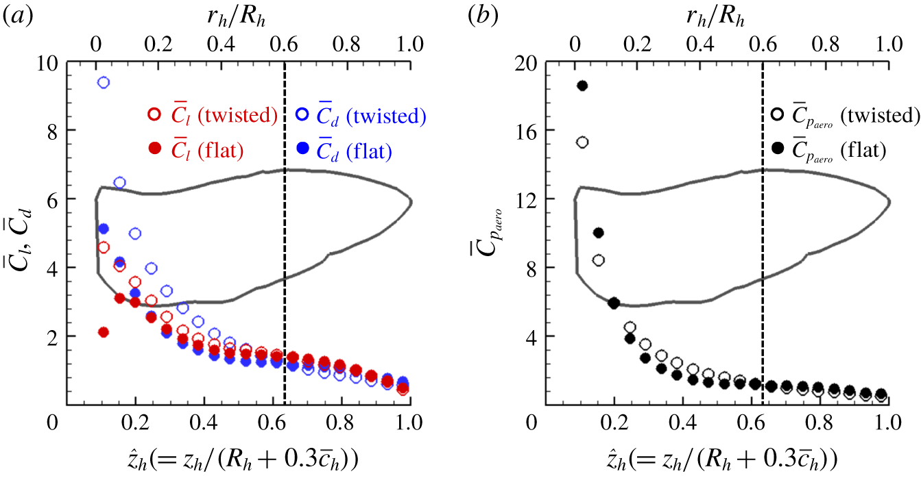
 $y_{s}$-direction, figure 8b) and opposite to the wing moving directions, respectively. Figure 10 shows the spanwise variations of the time-averaged (
 $4\leqslant t/T<5$) sectional lift, drag and aerodynamic power coefficients on the wing element (
 $c\unicode[STIX]{x0394}z$) of the flat and twisted hind wings, where
 $\overline{C}_{l}=2\unicode[STIX]{x0394}\overline{L}/\unicode[STIX]{x1D70C}(z\dot{\unicode[STIX]{x1D719}}_{rms})^{2}c\unicode[STIX]{x0394}z$,
 $\overline{C}_{d}=2\unicode[STIX]{x0394}\overline{D}/\unicode[STIX]{x1D70C}(z\dot{\unicode[STIX]{x1D719}}_{rms})^{2}c\unicode[STIX]{x0394}z$,
 $\overline{C}_{p_{aero}}=2\unicode[STIX]{x0394}\overline{P}_{aero}/\unicode[STIX]{x1D70C}(z\dot{\unicode[STIX]{x1D719}}_{crmc})^{3}c\unicode[STIX]{x0394}z$,
 $c$ is the local chord length,
 $\dot{\unicode[STIX]{x1D719}}_{rms}=(\overline{|\dot{\unicode[STIX]{x1D719}}|^{2}})^{1/2}$ and
 $\dot{\unicode[STIX]{x1D719}}_{crmc}=(\overline{|\dot{\unicode[STIX]{x1D719}}|^{3}})^{1/3}$, respectively. Note that the sectional aerodynamic coefficients are denoted by using lower-case subscripts such as
 $C_{l}$, whereas the total aerodynamic coefficients are by using upper-case subscripts such as
 $C_{L}$. At the wing inner part (
 $r/R<0.6$), mainly due to high angles of attack, the sectional lift, drag and aerodynamic power coefficients of the twisted wing are larger (except very near the wing root for the power coefficient) than those of the flat one, whereas they are smaller at the outer part (
 $r/R\geqslant 0.6$) due to lower angles of attack. Nevertheless, the time-averaged total lift, drag and power are similar to each other.
Angle of attack and aerodynamic force and power coefficients of the rigid flat and twisted hind wings, respectively: (a) angle of attack,  $\unicode[STIX]{x1D6FC}$, of the hind wing; (b) definition of
 $\unicode[STIX]{x1D6FC}$ in the absence of deviation motion,
 $\unicode[STIX]{x1D703}=0^{\circ }$; (c) horizontal force; (d) vertical force; (e) aerodynamic power. In (b), a wing cross-section is shown in light blue with the leading edge marked with a solid circle. In (c–e), ——, flat (case 1); – – –, twisted (case 4).

Instantaneous vortical structures and pressure around the hind wing at $t/T=4.5$: (a) flat wing (case 1); (b) twisted wing (case 4). The contours of the instantaneous pressure on the suction surface of the hind wing are also plotted in this figure. The
 $\unicode[STIX]{x1D706}_{2}$ isosurfaces and colour contours are the same as those in figure 6.

Spanwise variations of time-averaged ( $4\leqslant t/T<5$) sectional lift, drag and aerodynamic power coefficients of the flat and twisted hind wings (cases 1 and 4): (a) lift and drag; (b) power. The planform shape of the hind wing is also plotted.

The mean vertical forces ( $\overline{F}_{Y}$) generated and aerodynamic power (
 $\overline{P}_{aero}$) required for cases 1 to 6 are given in table 3, together with the hovering efficiencies (
 $\unicode[STIX]{x1D702}_{a}=\overline{C}_{F_{Y}}^{3/2}/(\sqrt{2\unicode[STIX]{x1D6F7}_{h}AR_{h}\cos \unicode[STIX]{x1D6FD}_{h}}\,\overline{C}_{P_{aero}})$). The hovering efficiency is defined as the ratio of the ideal Rankine–Froude induced power to the actual aerodynamic power (Ellington Reference Ellington1984c; Usherwood & Lehmann Reference Usherwood and Lehmann2008). For cases 3 (hind wings, elytra and body) and 6 (the flat and twisted wings), the total vertical forces generated (57.1 and 56.5 mN) are quite similar to the weight of a beetle (58.2 mN), showing less than 3 % differences. When we consider the hind wing only (cases 1 and 4), due to the wing twisting, the vertical force is increased by 2.8 %, the aerodynamic power is decreased by 2.8 %, and the hovering efficiency is increased by 7.1 %, respectively, indicating a positive but small effect of the wing twist on the aerodynamic performance. A similar positive effect of the wing twist has been reported in the previous studies (Truong et al. Reference Truong, Phan, Park and Ko2013a; Phan et al. Reference Phan, Truong and Park2017), although the amounts of power reduction were different from the present one owing to different wing kinematics.
The vertical forces and aerodynamic power from the hind wing are very similar to the total magnitudes for all cases. The negligible effect of the elytron on the vertical force generation can be explained by a scaling law (Lee, Choi & Kim Reference Lee, Choi and Kim2015b): the mean vertical force acting on a flapping wing is scaled as
 $$\begin{eqnarray}\overline{F}_{Y}\sim \unicode[STIX]{x1D70C}\unicode[STIX]{x1D6F7}R^{2}f^{2}\overline{c}^{2}AR\sin 2\unicode[STIX]{x1D6FC}\cos \unicode[STIX]{x1D6FD}/(AR+2).\end{eqnarray}$$
With  $\unicode[STIX]{x1D6F7}_{h}\approx 5.6\unicode[STIX]{x1D6F7}_{e}$,
 $R_{h}\approx 1.51R_{e}$,
 $f_{h}=f_{e}$,
 $\overline{c}_{h}\approx \overline{c}_{e}$,
 $\unicode[STIX]{x1D6FC}_{h}\approx 47^{\circ }$,
 $\unicode[STIX]{x1D6FC}_{e}\approx 87^{\circ }$,
 $\cos \unicode[STIX]{x1D6FD}_{h}\approx \cos \unicode[STIX]{x1D6FD}_{e}$ and
 $AR_{h}\approx 1.56AR_{e}$ (see § 2 and table 1),
 $\overline{F}_{Y}$ (elytron)
 ${\sim}0.01\overline{F}_{Y}$ (hind wing) and thus it can be estimated that the motion of the elytron cannot generate a vertical force comparable to that by the hind wing.
5 Quasi-steady aerodynamic model of a flapping wing in hover
In this section, we develop an analytical model to predict the aerodynamic force and power by the flapping motion of the hind wing. As we already discussed in § 4, the aerodynamic forces by the body and elytron are negligible as compared to those by the hind wing, and thus we do not consider the contributions from the body and elytron in this section. We showed in the previous section that the twisted hind wing produces the sectional aerodynamic force and power different from those of the rigid flat hind wing. Nonetheless, because of difficulties in modelling the aerodynamic force and power of the twisted wing, we consider a rigid flat wing in developing an aerodynamic model. Due to this limitation, the aerodynamic performance of the hind wing of the beetle cannot be fully considered. However, we believe that the present model would aid in capturing essential mechanisms for the force generation and power expenditure of the beetle because the total force generated and power required by the rigid flat hind wing are very similar to those by the twisted hind wing (although the details of the sectional coefficients are different near the root for two wings). We also assume that the interaction between left and right hind wings is insignificant, and develop an aerodynamic model for a single wing considering the symmetry between the left and right wings. We include the effects of the LEV and WTV, wing–wake interaction, wing acceleration and deceleration, wing pitching motion, and wing shape, and suggest a predictive quasi-steady blade element theory combined with the momentum theory. Unless otherwise required, we hereafter omit the subscript  $h$ that represents the hind wing.
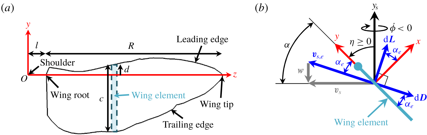
Wing parameters used for the blade element theory (hind wing): (a) wing shape; (b) angles and sectional forces. In (b), a wing cross-section is shown in light blue with the leading edge denoted as a solid circle, and  $w$ is the downwash motion.

5.1 Quasi-steady blade element theory
The blade element theory, originally applied to flapping flight by Osborne (Reference Osborne1951), has been used to evaluate the force on a flapping wing by dividing it into several elements and integrating their forces over the whole wing (Sane & Dickinson Reference Sane and Dickinson2002; Berman & Wang Reference Berman and Wang2007; Whitney & Wood Reference Whitney and Wood2010; Nakata et al. Reference Nakata, Liu and Bomphrey2015; Wang et al. Reference Wang, Goosen and van Keulen2016). Figure 11 shows the parameters used for the blade element theory. Here,  $c$ is the local chord length and
 $d$ is the position of the leading edge from the pitching axis. The (
 $x,y,z$) coordinate is fixed to the wing shoulder, and the offset distance (distance between the wing shoulder and root) is denoted as
 $l(=0.3\overline{c}_{h})$.
In the absence of the out-of-plane motion ( $\unicode[STIX]{x1D703}=\dot{\unicode[STIX]{x1D703}}=\ddot{\unicode[STIX]{x1D703}}=0$), the wing angular velocity (
 $\unicode[STIX]{x1D74E}$) can be represented as
 $$\begin{eqnarray}\displaystyle \unicode[STIX]{x1D74E} & = & \displaystyle \dot{\unicode[STIX]{x1D719}}\boldsymbol{e}_{y_{s}}+\dot{\unicode[STIX]{x1D702}}\boldsymbol{e}_{z}\nonumber\\ \displaystyle & = & \displaystyle \dot{\unicode[STIX]{x1D719}}\sin \unicode[STIX]{x1D702}\boldsymbol{e}_{x}+\dot{\unicode[STIX]{x1D719}}\cos \unicode[STIX]{x1D702}\boldsymbol{e}_{y}+\dot{\unicode[STIX]{x1D702}}\boldsymbol{e}_{z},\end{eqnarray}$$
where  $\unicode[STIX]{x1D719}$ is the sweeping angle on the stroke plane,
 $\unicode[STIX]{x1D702}$ is the pitching angle, and
 $\boldsymbol{e}_{i}$ is the unit vector in
 $i$ direction. From (5.1), the angular acceleration (
 $\unicode[STIX]{x1D74D}$) is obtained as
 $$\begin{eqnarray}\unicode[STIX]{x1D74D}=\dot{\unicode[STIX]{x1D74E}}=(\ddot{\unicode[STIX]{x1D719}}\sin \unicode[STIX]{x1D702}+\dot{\unicode[STIX]{x1D719}}\dot{\unicode[STIX]{x1D702}}\cos \unicode[STIX]{x1D702})\boldsymbol{e}_{x}+(\ddot{\unicode[STIX]{x1D719}}\cos \unicode[STIX]{x1D702}-\dot{\unicode[STIX]{x1D719}}\dot{\unicode[STIX]{x1D702}}\sin \unicode[STIX]{x1D702})\boldsymbol{e}_{y}+\ddot{\unicode[STIX]{x1D702}}\boldsymbol{e}_{z}.\end{eqnarray}$$
With (5.1) and (5.2), the sectional wing sweeping velocity and acceleration of an infinitesimally thin wing (i.e.  $x=0$ on the wing) at
 $y=0$ (
 $\boldsymbol{v}_{s}$ and
 $\boldsymbol{a}_{s}$, respectively), are obtained as
 $$\begin{eqnarray}\left.\begin{array}{@{}c@{}}\displaystyle \boldsymbol{v}_{s}=\unicode[STIX]{x1D74E}\times z\boldsymbol{e}_{z}=z(\unicode[STIX]{x1D714}_{y}\boldsymbol{e}_{x}-\unicode[STIX]{x1D714}_{x}\boldsymbol{e}_{y}),\\ \displaystyle \begin{array}{@{}rcl@{}}\displaystyle \boldsymbol{a}_{s}\; & =\; & \displaystyle \unicode[STIX]{x1D74D}\times z\boldsymbol{e}_{z}+\unicode[STIX]{x1D74E}\times \boldsymbol{v}_{s}\\ \; & =\; & \displaystyle z[(\unicode[STIX]{x1D714}_{z}\unicode[STIX]{x1D714}_{x}+\unicode[STIX]{x1D713}_{y})\boldsymbol{e}_{x}+(\unicode[STIX]{x1D714}_{y}\unicode[STIX]{x1D714}_{z}-\unicode[STIX]{x1D713}_{x})\boldsymbol{e}_{y}-(\unicode[STIX]{x1D714}_{x}^{2}+\unicode[STIX]{x1D714}_{y}^{2})\boldsymbol{e}_{z}].\end{array}\end{array}\right\}\end{eqnarray}$$
When  $|\boldsymbol{v}_{s}|\neq 0$, the angle of attack (
 $\unicode[STIX]{x1D6FC}$) can be defined as
 $$\begin{eqnarray}\unicode[STIX]{x1D6FC}=\arccos \left(\frac{\boldsymbol{v}_{s}\boldsymbol{\cdot }\boldsymbol{e}_{y}}{|\boldsymbol{v}_{s}|}\right)\quad \text{for }0\leqslant \unicode[STIX]{x1D6FC}\leqslant \unicode[STIX]{x03C0}.\end{eqnarray}$$
The wake behind a flapping wing may be approximated by a steady and non-uniform downwash velocity ( $\boldsymbol{w}$) normal to the stroke plane as
 $$\begin{eqnarray}\boldsymbol{w}=-w(z)\boldsymbol{e}_{y_{s}}\quad (w\geqslant 0).\end{eqnarray}$$
When a flapping wing interacts with a non-uniform downwash motion ( $\boldsymbol{w}$), the effective sectional wing velocity and angle of attack are given as
 $$\begin{eqnarray}\left.\begin{array}{@{}c@{}}\displaystyle \boldsymbol{v}_{s,e}=\boldsymbol{v}_{s}-\boldsymbol{w},\\ \displaystyle \unicode[STIX]{x1D6FC}_{e}=\arccos \left(\frac{\boldsymbol{v}_{s,e}\boldsymbol{\cdot }\boldsymbol{e}_{y}}{|\boldsymbol{v}_{s,e}|}\right)\end{array}\quad \text{for }0\leqslant \unicode[STIX]{x1D6FC}_{e}\leqslant \unicode[STIX]{x03C0}.\right\}\end{eqnarray}$$
With the assumption of no radial force, the required aerodynamic torque ( $\text{d}\unicode[STIX]{x1D749}$) and power (
 $\text{d}P_{aero}$) on a wing sectional element are given by
 $$\begin{eqnarray}\left.\begin{array}{@{}c@{}}\displaystyle \text{d}\unicode[STIX]{x1D749}=z\,\text{d}F_{y}\boldsymbol{e}_{x}-z\,\text{d}F_{x}\boldsymbol{e}_{y}+y_{cp}\,\text{d}F_{x}\boldsymbol{e}_{z},\\ \displaystyle \text{d}P_{aero}=\text{d}\unicode[STIX]{x1D749}\boldsymbol{\cdot }\unicode[STIX]{x1D74E},\end{array}\right\}\end{eqnarray}$$
where  $\text{d}\boldsymbol{F}$ is the force on the wing sectional element, and
 $y_{cp}$ is the location of centre of pressure from the pitching axis.
The sectional aerodynamic force on a flapping wing is decomposed into four different components due to the sweeping (swp) and pitching (pit) motions, their coupling (cpl) and added mass effect (add) which is further decomposed into two components owing to the sweeping (add, 1) and pitching (add, 2) accelerations, respectively. Then, the aerodynamic force, torque and power of a flapping wing are given as
 $$\begin{eqnarray}\left.\begin{array}{@{}c@{}}\displaystyle \boldsymbol{F}(t)=\int [(\text{d}F_{x}^{swp}+\text{d}F_{x}^{pit}+\text{d}F_{x}^{cpl}+\text{d}F_{x}^{add,1}+\text{d}F_{x}^{add,2})\boldsymbol{e}_{x}+\text{d}F_{y}^{swp}\boldsymbol{e}_{y}],\\ \displaystyle \begin{array}{@{}rcl@{}}\displaystyle \unicode[STIX]{x1D749}(t)\; & =\; & \displaystyle \int [\!z\,\text{d}F_{y}^{swp}\boldsymbol{e}_{x}-z(\text{d}F_{x}^{swp}+\text{d}F_{x}^{pit}+\text{d}F_{x}^{cpl}+\text{d}F_{x}^{add,1}+\text{d}F_{x}^{add,2})\boldsymbol{e}_{y}\\ \; & \; & \displaystyle +\,(y_{cp}^{swp}\,\text{d}F_{x}^{swp}+y_{cp}^{pit}\,\text{d}F_{x}^{pit}+y_{cp}^{cpl}\,\text{d}F_{x}^{cpl}+y_{cp}^{add,1}\,\text{d}F_{x}^{add,1}+y_{cp}^{add,2}\,\text{d}F_{x}^{add,2})\boldsymbol{e}_{z}\! ],\end{array}\\ \displaystyle P_{aero}(t)=\unicode[STIX]{x1D749}\boldsymbol{\cdot }\unicode[STIX]{x1D74E}.\end{array}\right\}\end{eqnarray}$$
In this equation, we take  $\text{d}F_{y}^{pit}=\text{d}F_{y}^{cpl}=\text{d}F_{y}^{add,1}=\text{d}F_{y}^{add,2}=0$ from the assumptions of infinitesimally thin wing and neglected viscous forces due to the absence of viscous theory. As shown below (§ 6), even with these assumptions, the prediction performance is not degraded.
The lift and drag forces on the flapping wing are
 $$\begin{eqnarray}\left.\begin{array}{@{}c@{}}\displaystyle L=F_{x}\sin \unicode[STIX]{x1D702}+F_{y}\cos \unicode[STIX]{x1D702},\\ D=-\text{sgn}(\dot{\unicode[STIX]{x1D719}})(F_{x}\cos \unicode[STIX]{x1D702}-F_{y}\sin \unicode[STIX]{x1D702}).\end{array}\right\}\end{eqnarray}$$
The components of the sectional aerodynamic force and the corresponding locations of centre of pressure are given as follows (Andersen, Pesavento & Wang Reference Andersen, Pesavento and Wang2005; Whitney & Wood Reference Whitney and Wood2010; Wang et al. Reference Wang, Goosen and van Keulen2016):
 $$\begin{eqnarray}\left.\begin{array}{@{}c@{}}\displaystyle \text{d}F_{x}^{swp}=-\frac{1}{2}\text{sgn}(\boldsymbol{v}_{s,e}\boldsymbol{\cdot }\boldsymbol{e}_{x})\unicode[STIX]{x1D70C}c|\boldsymbol{v}_{s,e}|^{2}(C_{l}\cos \unicode[STIX]{x1D6FC}_{e}+C_{d}\sin \unicode[STIX]{x1D6FC}_{e})\,\text{d}z,\\ \displaystyle \text{d}F_{y}^{swp}=\frac{1}{2}\unicode[STIX]{x1D70C}c|\boldsymbol{v}_{s,e}|^{2}(C_{l}\sin \unicode[STIX]{x1D6FC}_{e}-C_{d}\cos \unicode[STIX]{x1D6FC}_{e})\,\text{d}z,\quad y_{cp}^{swp}=d-\frac{c}{\unicode[STIX]{x03C0}}|\unicode[STIX]{x1D6FC}_{e}|,\end{array}\right\}\end{eqnarray}$$
 $$\begin{eqnarray}\text{d}F_{x}^{pit}=\displaystyle \frac{1}{6}\unicode[STIX]{x1D70C}\unicode[STIX]{x1D714}_{z}|\unicode[STIX]{x1D714}_{z}|C_{pit}[d^{3}+(d-c)^{3}]\,\text{d}z,\quad y_{cp}^{pit}=\frac{3}{4}\frac{d^{4}+(d-c)^{4}}{d^{3}+(d-c)^{3}},\end{eqnarray}$$
 $$\begin{eqnarray}\text{d}F_{x}^{cpl}=\left\{\begin{array}{@{}ll@{}}\displaystyle -\unicode[STIX]{x03C0}\unicode[STIX]{x1D70C}\left(\frac{3}{4}c-d\right)c(\boldsymbol{v}_{s,e}\boldsymbol{\cdot }\boldsymbol{e}_{y})\unicode[STIX]{x1D714}_{z}\,\text{d}z,\quad y_{cp}^{cpl}=d-\frac{1}{4}c & \text{for }\boldsymbol{v}_{s,e}\boldsymbol{\cdot }\boldsymbol{e}_{y}\geqslant 0,\\ \displaystyle -\unicode[STIX]{x03C0}\unicode[STIX]{x1D70C}\left(d-\frac{1}{4}c\right)c(\boldsymbol{v}_{s,e}\boldsymbol{\cdot }\boldsymbol{e}_{y})\unicode[STIX]{x1D714}_{z}\,\text{d}z,\quad y_{cp}^{cpl}=d-\frac{3}{4}c & \text{for }\boldsymbol{v}_{s,e}\boldsymbol{\cdot }\boldsymbol{e}_{y}<0,\end{array}\right\}\end{eqnarray}$$
 $$\begin{eqnarray}\left.\begin{array}{@{}c@{}}\displaystyle \text{d}F_{x}^{add,1}=-\frac{1}{4}\unicode[STIX]{x03C0}\unicode[STIX]{x1D70C}c^{2}(\boldsymbol{a}_{s}\boldsymbol{\cdot }\boldsymbol{e}_{x})\,\text{d}z,\quad y_{cp}^{add,1}=d-\frac{1}{2}c,\\ \displaystyle \text{d}F_{x}^{add,2}=-\frac{1}{4}\unicode[STIX]{x03C0}\unicode[STIX]{x1D70C}c^{2}\left(\frac{1}{2}c-d\right)\unicode[STIX]{x1D713}_{z}\,\text{d}z,\quad y_{cp}^{add,2}=d-\frac{(9c-16d)c}{16c-32d},\end{array}\right\}\end{eqnarray}$$
where  $C_{l}$ and
 $C_{d}$ are the sectional lift and drag coefficients of a revolving wing, respectively,
 $C_{pit}$ is the force coefficient due to the pitching motion,
 $d$ is the position of the leading edge from the pitching axis and
 $\unicode[STIX]{x1D713}_{z}$ is the pitching acceleration (5.2). Note that (5.10)–(5.13) are the same as those of Wang et al. (Reference Wang, Goosen and van Keulen2016) when
 $\boldsymbol{v}_{s,e}=\boldsymbol{v}_{s}$ and
 $\unicode[STIX]{x1D6FC}_{e}=\unicode[STIX]{x1D6FC}$ in (5.10) and (5.12). However, we use different formulae for
 $C_{l}$,
 $C_{d}$ and
 $C_{pit}$ (see below) and do not include the Coriolis effect in
 $\text{d}F_{x}^{cpl}$ because the translational velocity of a flapping wing is typically a few times the rotational velocity (Wang et al. Reference Wang, Goosen and van Keulen2016).
The conventional definitions of the lift ( $L$) and drag (
 $D$) coefficients for a flat wing revolving at a constant angular velocity
 $\unicode[STIX]{x1D6FA}$ are
 $$\begin{eqnarray}C_{L}=\frac{2L}{\unicode[STIX]{x1D70C}\hat{z}_{2}^{2}(R+l)^{2}\unicode[STIX]{x1D6FA}^{2}R\overline{c}},\quad C_{D}=\frac{2D}{\unicode[STIX]{x1D70C}\hat{z}_{2}^{2}(R+l)^{2}\unicode[STIX]{x1D6FA}^{2}R\overline{c}},\end{eqnarray}$$
where  $\hat{z}_{k}(=\sqrt[k]{\int _{1-\unicode[STIX]{x1D706}}^{1}{\hat{c}}\hat{z}^{k}\,\text{d}\hat{z}/\unicode[STIX]{x1D706}})$ is a non-dimensional radius of the
 $k$th moment of wing area,
 ${\hat{c}}=c/\overline{c}$,
 $\hat{z}=z/(R+l)$ and
 $\unicode[STIX]{x1D706}=R/(R+l)$. Wang et al. (Reference Wang, Birch and Dickinson2004) suggested
 $$\begin{eqnarray}\left.\begin{array}{@{}c@{}}\displaystyle C_{L}=A\sin 2\unicode[STIX]{x1D6FC},\\ \displaystyle C_{D}=B-C\cos 2\unicode[STIX]{x1D6FC},\end{array}\right\}\end{eqnarray}$$
where  $A$,
 $B$ and
 $C$ are model constants determined from experimental or numerical data, and depend on the Reynolds number and wing geometry. Taha, Hajj & Beran (Reference Taha, Hajj and Beran2014) provided a theoretical value for
 $A$ in (5.15) based on the extended lifting line theory (Schlichting & Truckenbrodt Reference Schlichting and Truckenbrodt1979), and suggested
 $$\begin{eqnarray}C_{L}=\unicode[STIX]{x03C0}\frac{AR}{\sqrt{AR^{2}+4}+2}\sin 2\unicode[STIX]{x1D6FC}.\end{eqnarray}$$
They showed that (5.16) is an excellent predictive model for  $0\leqslant \unicode[STIX]{x1D6FC}\leqslant \unicode[STIX]{x03C0}/2$. Note that this formula includes the effect of WTV as well as LEV (Wang et al. Reference Wang, Birch and Dickinson2004; Berman & Wang Reference Berman and Wang2007; Taha et al. Reference Taha, Hajj and Beran2014; Wang et al. Reference Wang, Goosen and van Keulen2016).
The sectional lift and drag coefficients of a revolving wing are defined by
 $$\begin{eqnarray}C_{l}=\displaystyle \frac{2\,\text{d}L}{\unicode[STIX]{x1D70C}z^{2}\unicode[STIX]{x1D6FA}^{2}c\,\text{d}z},\quad C_{d}=\frac{2\,\text{d}D}{\unicode[STIX]{x1D70C}z^{2}\unicode[STIX]{x1D6FA}^{2}c\,\text{d}z},\end{eqnarray}$$
where  $\text{d}L$ and
 $\text{d}D$ are the sectional lift and drag forces acting on
 $c\,\text{d}z$. When we assume
 $C_{l}=K\hat{z}^{n}$ (
 $K$ is a proportional constant),
 $L=\int _{l}^{l+R}(1/2)K\unicode[STIX]{x1D70C}z^{2}\unicode[STIX]{x1D6FA}^{2}c\hat{z}^{n}\,\text{d}z=(1/2)K\unicode[STIX]{x1D70C}(l+R)^{2}\unicode[STIX]{x1D6FA}^{2}R\overline{c}\int _{1-\unicode[STIX]{x1D706}}^{1}{\hat{c}}\hat{z}^{n+2}\,\text{d}\hat{z}/\unicode[STIX]{x1D706}=(1/2)K\unicode[STIX]{x1D70C}(l+R)^{2}\unicode[STIX]{x1D6FA}^{2}R\overline{c}\hat{z}_{n+2}^{n+2}$, from which the proportional constant
 $K$ is obtained as
 $K=\hat{z}_{2}^{2}C_{L}/\hat{z}_{n+2}^{n+2}$. Therefore, the sectional lift coefficient of a revolving wing can be estimated by non-dimensional radii of the second and (
 $n+2$)th moments of wing area and
 $C_{L}$ if
 $C_{l}\sim \hat{z}^{n}$,
 $$\begin{eqnarray}C_{l}=\frac{\hat{z}_{2}^{2}}{\hat{z}_{n+2}^{n+2}}\hat{z}^{n}C_{L}.\end{eqnarray}$$
Wang et al. (Reference Wang, Goosen and van Keulen2016) assumed that  $C_{l}$ is constant along the radial direction, i.e.
 $n=0$; then,
 $C_{l}=C_{L}$. Some other studies showed that
 $n\approx -1$ for a low-aspect-ratio revolving wing at low Reynolds number and high angles of attack (Poelma, Dickson & Dickinson Reference Poelma, Dickson and Dickinson2006; Kim, Kweon & Choi Reference Kim, Kweon and Choi2015). We use
 $n=-1$ to estimate
 $C_{l}$, because
 $n=0$ may be valid for a high-aspect-ratio revolving wing operating at high Reynolds number and low angles of attack.
Wang et al. (Reference Wang, Goosen and van Keulen2016) provided a model for the drag coefficient from (5.16) assuming that the total force on the wing is normal to the wing surface,
 $$\begin{eqnarray}C_{D}=C_{L}\tan \unicode[STIX]{x1D6FC}=\frac{2\unicode[STIX]{x03C0}AR}{\sqrt{AR^{2}+4}+2}\sin ^{2}\unicode[STIX]{x1D6FC}.\end{eqnarray}$$
They also assumed  $C_{d}=C_{D}$, as done for the sectional lift coefficient. Recently, Oh & Choi (Reference Oh and Choi2018) suggested an improved model for the drag coefficient as follows:
 $$\begin{eqnarray}C_{D}=\frac{1}{\unicode[STIX]{x1D706}\hat{z}_{2}^{2}}\left(\frac{2.656}{Re^{1/2}}\unicode[STIX]{x1D705}_{1}+\frac{5.32}{Re^{7/8}}\unicode[STIX]{x1D705}_{2}\right)\cos 2\unicode[STIX]{x1D6FC}+\frac{2\unicode[STIX]{x03C0}AR}{\sqrt{AR^{2}+4}+2}\sin ^{2}\unicode[STIX]{x1D6FC},\end{eqnarray}$$
where  $Re=(l+R)\unicode[STIX]{x1D6FA}\overline{c}/\unicode[STIX]{x1D708}$,
 $\unicode[STIX]{x1D705}_{1}=\int _{1-\unicode[STIX]{x1D706}}^{1}{\hat{c}}^{1/2}\hat{z}^{3/2}\,\text{d}\hat{z}$ and
 $\unicode[STIX]{x1D705}_{2}=\int _{1-\unicode[STIX]{x1D706}}^{1}{\hat{c}}^{1/8}\hat{z}^{9/8}\,\text{d}\hat{z}$. The first term in (5.20) is the contribution of viscous drag for a low-Reynolds-number revolving wing (
 $Re\sim O(10^{2})$), and the second term is the same as (5.19). Equations (5.16) and (5.20) provided excellent agreement with the measured
 $C_{L}$ and
 $C_{D}$ of revolving fruit fly, hawkmoth and bumblebee wings for the ranges of
 $2.83\leqslant AR\leqslant 3.74$ and
 $136\leqslant Re\leqslant 8071$. In the present study, we assume that
 $C_{d}$ is also in the form of
 $C_{d}=B^{\ast }-C^{\ast }\cos 2\unicode[STIX]{x1D6FC}$ as in (5.15). To determine
 $B^{\ast }$ and
 $C^{\ast }$, we consider the sectional drag coefficients at
 $\unicode[STIX]{x1D6FC}=0$ and
 $\unicode[STIX]{x03C0}/4$, as done in Oh & Choi (Reference Oh and Choi2018):
 $C_{d}(0)=2.656/Re_{c}^{1/2}+5.32/Re_{c}^{7/8}$ (
 $Re_{c}=z\unicode[STIX]{x1D6FA}c/\unicode[STIX]{x1D708}$) from the triple deck theory (Stewartson Reference Stewartson1968; Messiter Reference Messiter1970), and
 $C_{d}(\unicode[STIX]{x03C0}/4)=C_{l}(\unicode[STIX]{x03C0}/4)$ because the resultant force on the wing element at
 $\unicode[STIX]{x1D6FC}=\unicode[STIX]{x03C0}/4$ (a post-stall angle) is nearly perpendicular to the wing chord. Then, our model for the sectional lift and drag coefficients of a revolving wing becomes
 $$\begin{eqnarray}\left.\begin{array}{@{}c@{}}\displaystyle C_{l}=\frac{\hat{z}_{2}^{2}}{\hat{z}_{1}}\frac{\unicode[STIX]{x03C0}AR}{\sqrt{AR^{2}+4}+2}\frac{\sin 2\unicode[STIX]{x1D6FC}}{\hat{z}},\\ \displaystyle C_{d}=\left(\frac{2.656}{Re_{c}^{1/2}}+\frac{5.32}{Re_{c}^{7/8}}\right)\cos 2\unicode[STIX]{x1D6FC}+\frac{\hat{z}_{2}^{2}}{\hat{z}_{1}}\frac{2\unicode[STIX]{x03C0}AR}{\sqrt{AR^{2}+4}+2}\frac{\sin ^{2}\unicode[STIX]{x1D6FC}}{\hat{z}}.\end{array}\right\}\end{eqnarray}$$
In the present study, we use (5.21) for  $C_{l}$ and
 $C_{d}$ in (5.10), together with
 $Re_{c}=|\boldsymbol{v}_{s,e}|c/\unicode[STIX]{x1D708}$ and
 $\unicode[STIX]{x1D6FC}$ replaced by
 $\unicode[STIX]{x1D6FC}_{e}$.
Now  $C_{pit}$ has been commonly modelled as the drag coefficient of a wing at
 $\unicode[STIX]{x1D6FC}=\unicode[STIX]{x03C0}/2$ (Andersen et al. Reference Andersen, Pesavento and Wang2005; Whitney & Wood Reference Whitney and Wood2010; Nakata et al. Reference Nakata, Liu and Bomphrey2015; Wang et al. Reference Wang, Goosen and van Keulen2016). Note that Whitney & Wood (Reference Whitney and Wood2010), Nakata et al. (Reference Nakata, Liu and Bomphrey2015) and Wang et al. (Reference Wang, Goosen and van Keulen2016) took
 $C_{pit}$ as the drag coefficient of a wing at
 $\unicode[STIX]{x1D6FC}=\unicode[STIX]{x03C0}/2$ revolving about the
 $y_{s}$-axis rather than about the
 $z$-axis: e.g.
 $C_{pit}=2\unicode[STIX]{x03C0}AR/(\sqrt{AR^{2}+4}+2)$ from (5.19) at
 $\unicode[STIX]{x1D6FC}=\unicode[STIX]{x03C0}/2$ in Wang et al. (Reference Wang, Goosen and van Keulen2016). According to Ellington (Reference Ellington1991), the drag coefficient of a two-dimensional flat plate at
 $\unicode[STIX]{x1D6FC}=\unicode[STIX]{x03C0}/2$ is empirically given as
 $C_{d}=1.95+50/Re$. Therefore, we use
 $$\begin{eqnarray}C_{pit}=2.0\end{eqnarray}$$
as done in Andersen et al. (Reference Andersen, Pesavento and Wang2005), although the flapping wing under consideration is not two-dimensional.
5.2 Estimation of induced downwash motion
To obtain the non-uniform downwash motion  $\boldsymbol{w}$ defined in (5.5), we combine the present blade element theory with an inviscid momentum theory (Ellington Reference Ellington1984b; Johnson Reference Johnson1994). From the momentum theory, the ideal (without tip loss effect) period-averaged sectional lift (
 $\text{d}\overline{L}$) of a flapping wing is
 $$\begin{eqnarray}\text{d}\overline{L}=2\unicode[STIX]{x1D70C}\unicode[STIX]{x1D6F7}w^{2}z\,\text{d}z,\end{eqnarray}$$
where  $\unicode[STIX]{x1D6F7}$ is the sweeping amplitude of the flapping wing and
 $w(z)$ is a local downwash velocity. Now
 $\text{d}\overline{L}$ can be also obtained by the quasi-steady blade element theory: from (5.10)–(5.13) and the relationship in (5.9),
 $$\begin{eqnarray}\displaystyle \text{d}\overline{L} & = & \displaystyle \frac{1}{T}\int _{t_{0}}^{t_{0}+T}(\text{d}F_{x}\sin \unicode[STIX]{x1D702}+\text{d}F_{y}\cos \unicode[STIX]{x1D702})\,\text{d}t\nonumber\\ \displaystyle & = & \displaystyle \frac{1}{T}\int _{t_{0}}^{t_{0}+T} [(\text{d}F_{x}^{swp}+\text{d}F_{x}^{pit}+\text{d}F_{x}^{cpl}+\text{d}F_{x}^{add,1}+\text{d}F_{x}^{add,2})\sin \unicode[STIX]{x1D702}\nonumber\\ \displaystyle & & \displaystyle +\,\text{d}F_{y}^{swp}\cos \unicode[STIX]{x1D702}\!]\,\text{d}t.\end{eqnarray}$$
The downwash motion can be obtained by matching (5.23) with (5.24). However,  $w$ is nonlinearly coupled through
 $\text{d}\boldsymbol{F}^{swp}$ and
 $\text{d}\boldsymbol{F}^{cpl}$ as in (5.10) and (5.12). Thus, equations (5.23) and (5.24) should be solved by an iterative method or by a linearization of (5.24). We obtain
 $w$ by both approaches and find that their differences are negligible (see below). The assumptions for the linearization are the following:
(i) The resultant force on the wing is nearly perpendicular to the wing surface because flapping wings typically operate at high angles of attack and thus the viscous friction force is much smaller than the force due to pressure difference. Then, the first term of
 $C_{d}$ in (5.21) is neglected, which results in $\text{d}F_{y}^{swp}=0$ in (5.10).
(ii) Here
$|\text{tan}\,\unicode[STIX]{x1D702}|$ is of the order of 1 or less, and $\dot{\unicode[STIX]{x1D719}}\unicode[STIX]{x1D702}\leqslant 0$. These are valid for typical flapping flight of insects during most of the flapping period. For example, see figure 2(a). During advanced or delayed rotation, this assumption yields mispredictions of $\text{d}\boldsymbol{F}^{swp}$ and $\text{d}\boldsymbol{F}^{cpl}$, but does not cause a crucial error for estimation of $\text{d}\overline{L}$ in (5.24) if the duration of such rotation is short as compared to the whole cycle.(iii) Sectional sweeping speed is much faster than the speed of local downwash motion, i.e.
$|\boldsymbol{v}_{s}|(=|z\dot{\unicode[STIX]{x1D719}}|)\gg w$. Strictly, this is not valid near the wing root ($z\approx 0$) and during stroke reversal ($\dot{\unicode[STIX]{x1D719}}\approx 0$). In these cases, however, the sectional aerodynamic forces due to the sweeping velocity ($\text{d}\boldsymbol{F}^{swp}$ and $\text{d}\boldsymbol{F}^{cpl}$) are small. Therefore, albeit causing some discrepancies in sectional forces near the wing root, this assumption does not lead to a significant error in estimating the aerodynamic forces acting on the entire wing. For a similar reason, this assumption has been commonly used to estimate the downwash distribution of rotary wings (Johnson Reference Johnson1994; Usherwood & Ellington Reference Usherwood and Ellington2002; Leishman Reference Leishman2006).


It should be emphasized that the above assumptions are used only for linearization of (5.24) and derivation of an explicit form of  $w$.
The following relationships hold (figure 11b),
 $$\begin{eqnarray}\left.\begin{array}{@{}c@{}}\displaystyle \boldsymbol{w}\boldsymbol{\cdot }\boldsymbol{e}_{x}=-w\sin \unicode[STIX]{x1D702},\quad \boldsymbol{w}\boldsymbol{\cdot }\boldsymbol{e}_{y}=-w\cos \unicode[STIX]{x1D702},\\ \displaystyle \boldsymbol{v}_{s}\boldsymbol{\cdot }\boldsymbol{e}_{x}=z\dot{\unicode[STIX]{x1D719}}\cos \unicode[STIX]{x1D702},\quad \boldsymbol{v}_{s}\boldsymbol{\cdot }\boldsymbol{e}_{y}=-z\dot{\unicode[STIX]{x1D719}}\sin \unicode[STIX]{x1D702},\\ \displaystyle \sqrt{|\boldsymbol{v}_{s}|^{2}+w^{2}}\sin \unicode[STIX]{x1D6FC}_{e}=|\boldsymbol{v}_{s}|\text{sin}\,\unicode[STIX]{x1D6FC}-w\cos \unicode[STIX]{x1D6FC}.\end{array}\right\}\end{eqnarray}$$
With (5.10), (5.21) and assumption (i),  $\text{d}F_{x}^{swp}\sin \unicode[STIX]{x1D702}$ in (5.24) becomes
 $$\begin{eqnarray}\text{d}F_{x}^{swp}\sin \unicode[STIX]{x1D702}\approx -\text{sgn}(\boldsymbol{v}_{s,e}\boldsymbol{\cdot }\boldsymbol{e}_{x})\unicode[STIX]{x03C0}\unicode[STIX]{x1D70C}c(|\boldsymbol{v}_{s}|^{2}+w^{2})\sin \unicode[STIX]{x1D6FC}_{e}\sin \unicode[STIX]{x1D702}\frac{AR}{\sqrt{AR^{2}+4}+2}\frac{\hat{z}_{2}^{2}}{\hat{z}_{1}\hat{z}}\,\text{d}z.\end{eqnarray}$$
Assumptions (ii) and (iii), and (5.25) provide the following approximations:
 $$\begin{eqnarray}\left.\begin{array}{@{}c@{}}\displaystyle \text{sgn}(\boldsymbol{v}_{s,e}\boldsymbol{\cdot }\boldsymbol{e}_{x})=\text{sgn}(\boldsymbol{v}_{s}\boldsymbol{\cdot }\boldsymbol{e}_{x})\text{sgn}\left(1-\frac{\boldsymbol{w}\boldsymbol{\cdot }\boldsymbol{e}_{x}}{\boldsymbol{v}_{s}\boldsymbol{\cdot }\boldsymbol{e}_{x}}\right)\approx \text{sgn}(\boldsymbol{v}_{s}\boldsymbol{\cdot }\boldsymbol{e}_{x}),\\ \displaystyle (|\boldsymbol{v}_{s}|^{2}+w^{2})\sin \unicode[STIX]{x1D6FC}_{e}\simeq |\boldsymbol{v}_{s}|^{2}\sin \unicode[STIX]{x1D6FC}-w|\boldsymbol{v}_{s}|\text{cos}\,\unicode[STIX]{x1D6FC}.\end{array}\right\}\end{eqnarray}$$
Then, equation (5.26) can be further simplified by
 $$\begin{eqnarray}\displaystyle & & \displaystyle \text{d}F_{x}^{swp}\sin \unicode[STIX]{x1D702}\nonumber\\ \displaystyle & & \displaystyle \quad \approx \,-\text{sgn}(\boldsymbol{v}_{s}\boldsymbol{\cdot }\boldsymbol{e}_{x})\unicode[STIX]{x03C0}\unicode[STIX]{x1D70C}c(|\boldsymbol{v}_{s}|^{2}\sin \unicode[STIX]{x1D6FC}-w|\boldsymbol{v}_{s}|\text{cos}\,\unicode[STIX]{x1D6FC})\sin \unicode[STIX]{x1D702}\frac{AR}{\sqrt{AR^{2}+4}+2}\frac{\hat{z}_{2}^{2}}{\hat{z}_{1}\hat{z}}\,\text{d}z\nonumber\\ \displaystyle & & \displaystyle \quad \approx \,\text{d}F_{x}^{swp}|_{w=0}\sin \unicode[STIX]{x1D702}\nonumber\\ \displaystyle & & \displaystyle \qquad +\,w\underbrace{\left[\text{sgn}(\boldsymbol{v}_{s}\boldsymbol{\cdot }\boldsymbol{e}_{x})\unicode[STIX]{x03C0}\unicode[STIX]{x1D70C}c|\boldsymbol{v}_{s}|\cos \unicode[STIX]{x1D6FC}\sin \unicode[STIX]{x1D702}\frac{AR}{\sqrt{AR^{2}+4}+2}\frac{\hat{z}_{2}^{2}}{\hat{z}_{1}\hat{z}}\right]}_{\equiv \;I}\,\text{d}z.\end{eqnarray}$$
Here, it is noteworthy that  $I$ is always negative because
 $|\boldsymbol{v}_{s}|\text{cos}\,\unicode[STIX]{x1D6FC}=\boldsymbol{v}_{s}\boldsymbol{\cdot }\boldsymbol{e}_{y}$ from (5.4), and thus
 $\text{sgn}(\boldsymbol{v}_{s}\boldsymbol{\cdot }\boldsymbol{e}_{x})|\boldsymbol{v}_{s}|\text{cos}\,\unicode[STIX]{x1D6FC}=\text{sgn}(z\dot{\unicode[STIX]{x1D719}}\cos \unicode[STIX]{x1D702})(-z\dot{\unicode[STIX]{x1D719}}\sin \unicode[STIX]{x1D702})=-|z\dot{\unicode[STIX]{x1D719}}|\text{sin}\,\unicode[STIX]{x1D702}$ from (5.25). Therefore, the interactive effect of downwash and wing sweeping motions on the sectional lift (
 $wI\,\text{d}z$) is always negative. Assumption (ii) and (5.25) yield
 $$\begin{eqnarray}\text{sgn}(\boldsymbol{v}_{s,e}\boldsymbol{\cdot }\boldsymbol{e}_{y})=\text{sgn}(\boldsymbol{v}_{s}\boldsymbol{\cdot }\boldsymbol{e}_{y})\text{sgn}\left(1-\frac{\boldsymbol{w}\boldsymbol{\cdot }\boldsymbol{e}_{y}}{\boldsymbol{v}_{s}\boldsymbol{\cdot }\boldsymbol{e}_{y}}\right)\approx \text{sgn}(\boldsymbol{v}_{s}\boldsymbol{\cdot }\boldsymbol{e}_{y})=1.\end{eqnarray}$$
With (5.12) and (5.29),  $\text{d}F_{x}^{cpl}\sin \unicode[STIX]{x1D702}$ in (5.24) reduces to
 $$\begin{eqnarray}\displaystyle \text{d}F_{x}^{cpl}\sin \unicode[STIX]{x1D702} & {\approx} & \displaystyle -\unicode[STIX]{x03C0}\unicode[STIX]{x1D70C}\left(\frac{3}{4}c-d\right)c(\boldsymbol{v}_{s}\boldsymbol{\cdot }\boldsymbol{e}_{y}-\boldsymbol{w}\boldsymbol{\cdot }\boldsymbol{e}_{y})\unicode[STIX]{x1D714}_{z}\sin \unicode[STIX]{x1D702}\,\text{d}z\nonumber\\ \displaystyle & {\approx} & \displaystyle \text{d}F_{x}^{cpl}|_{w=0}\sin \unicode[STIX]{x1D702}-w\left[\unicode[STIX]{x03C0}\unicode[STIX]{x1D70C}\left(\frac{3}{4}c-d\right)c\dot{\unicode[STIX]{x1D702}}\sin \unicode[STIX]{x1D702}\cos \unicode[STIX]{x1D702}\right]\,\text{d}z.\end{eqnarray}$$
Substituting (5.28) and (5.30) into (5.24) provides an approximated period-averaged sectional lift from the blade element theory,
 $$\begin{eqnarray}\displaystyle \text{d}\overline{L} & {\approx} & \displaystyle w\overline{I}\,\text{d}z\nonumber\\ \displaystyle & & \displaystyle +\,\frac{1}{T}\int _{t_{0}}^{t_{0}+T}\sin \unicode[STIX]{x1D702}(\text{d}F_{x}^{swp}|_{w=0}+\text{d}F_{x}^{pit}+\text{d}F_{x}^{cpl}|_{w=0}+\text{d}F_{x}^{add,1}+\text{d}F_{x}^{add,2})\,\text{d}t\nonumber\\ \displaystyle & {\approx} & \displaystyle w\overline{I}\,\text{d}z+\text{d}\overline{L}|_{w=0}.\end{eqnarray}$$
Note that the second term in (5.30) disappears after the integration due to the periodicity of wing kinematics, i.e.  $\overline{\dot{\unicode[STIX]{x1D702}}\sin \unicode[STIX]{x1D702}\cos \unicode[STIX]{x1D702}}=0$. Also, from the assumption (i),
 $\text{d}F_{y}^{swp}|_{w=0}\approx 0$ and thus the integral in (5.31) becomes approximately the period-averaged sectional lift in the absence of downwash motion (
 $\text{d}\overline{L}|_{w=0}$).
Equating (5.31) with (5.23) provides a quadratic equation for  $w$,
 $$\begin{eqnarray}2\unicode[STIX]{x1D70C}\unicode[STIX]{x1D6F7}zw^{2}=\overline{I}w+\frac{\text{d}\overline{L}|_{w=0}}{\text{d}z}.\end{eqnarray}$$
The coefficients in (5.32) can be evaluated once wing geometry and kinematics are specified. Since  $I<0$,
 $\overline{I}<0$. Thus, unless the last term is negative (it is in general positive for insect flight),
 $w$ can be uniquely determined as
 $$\begin{eqnarray}w=\frac{1}{4\unicode[STIX]{x1D70C}\unicode[STIX]{x1D6F7}z}\left[\overline{I}+\left(\overline{I}^{2}+8\unicode[STIX]{x1D70C}\unicode[STIX]{x1D6F7}z\frac{\text{d}\overline{L}|_{w=0}}{\text{d}z}\right)^{1/2}\right]\geqslant 0\quad \text{for }z\neq 0.\end{eqnarray}$$
For the present wing geometry and kinematics, the maximum difference between (5.33), and iteratively obtained  $w$, is only
 $2.3\,\%$, and the time-averaged total lift, drag and power predicted with the latter are different from those with (5.33) by less than 1 %.
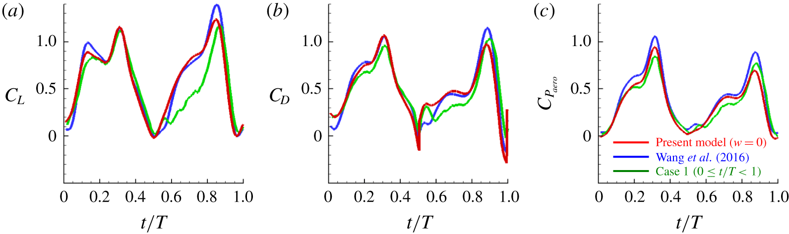
Predicted force and power coefficients using the present model with  $w=0$ and the model of Wang et al. (Reference Wang, Goosen and van Keulen2016), and those from the present numerical simulation during the first stroke period (case 1): (a) lift; (b) drag; (c) aerodynamic power.

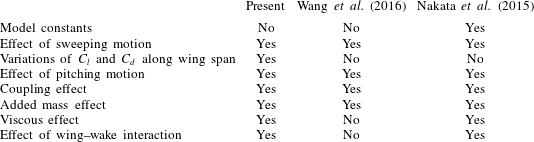
Comparison of the present quasi-steady model with the models by Wang et al. (Reference Wang, Goosen and van Keulen2016) and Nakata et al. (Reference Nakata, Liu and Bomphrey2015).

Table 4 summarizes the differences among the present model, a predictive model by Wang et al. (Reference Wang, Goosen and van Keulen2016) and a semi-empirical model by Nakata et al. (Reference Nakata, Liu and Bomphrey2015). The model of Nakata et al. (Reference Nakata, Liu and Bomphrey2015) contained model constants that were obtained by fitting them to predict their numerical results for a flapping hawkmoth wing during a quasi-periodic state. Thus, the effects of the fluid viscosity and wing–wake interaction were inherently included therein. However, their model constants depend on the wing geometry and should be determined whenever a wing geometry changes. Thus, their model is not entirely predictive. On the contrary, the predictive model suggested by Wang et al. (Reference Wang, Goosen and van Keulen2016) did not contain any model constants, but did not include the effects of friction force and wing–wake interaction. In the present study, we include the effect of wing–wake interaction, and consider the variations of  $C_{l}$ and
 $C_{d}$ along the wing span.
6 Model validation and discussions
In this section, we compare the forces and power ((5.8) and (5.9)) predicted by the present model ((5.10)–(5.13), (5.21) and (5.22)) together with  $w$ (5.33) for case 1 with those from the present numerical simulation and from the previous model by Wang et al. (Reference Wang, Goosen and van Keulen2016). Figure 12 shows the temporal variations of the lift, drag and aerodynamic power coefficients predicted by the present model with
 $w=0$ during the first stroke period (
 $0\leqslant t/T<1$), together with those from the present numerical simulation, and predicted by the model of Wang et al. (Reference Wang, Goosen and van Keulen2016). For the first half-stroke (
 $0\leqslant t/T<0.5$), both models show excellent prediction performance, although they slightly overestimate the force and power peaks. On the contrary, the predictions are poor (especially for
 $C_{L}$) during the second half-stroke (
 $0.5\leqslant t/T<1$) because of neglected induced downwash motion.
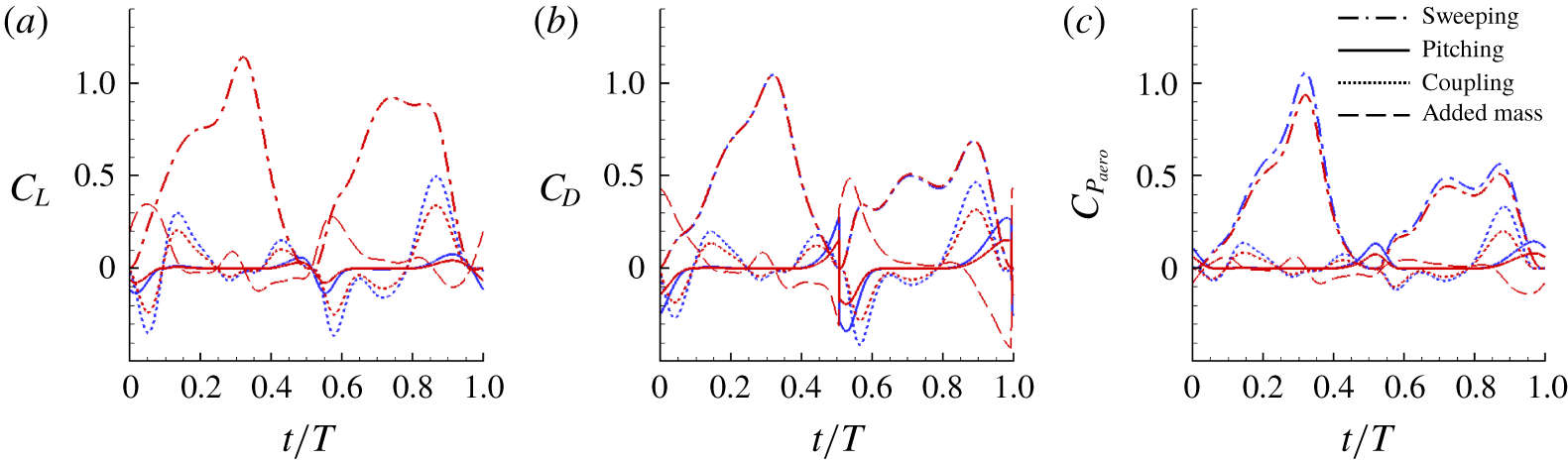
Predicted components of the force and power coefficients using the present model with  $w=0$ and the model of Wang et al. (Reference Wang, Goosen and van Keulen2016): (a) lift; (b) drag; (c) aerodynamic power. Red and blue lines denote the results predicted by the present model (
 $w=0$) and model of Wang et al. (Reference Wang, Goosen and van Keulen2016), respectively.

As shown in figure 13, the sweeping motion is the most dominant contributor to the force generation and power expenditure. The  $C_{L}$ due to the sweeping motion predicted by the present model is the same as that by the model of Wang et al. (Reference Wang, Goosen and van Keulen2016), although different
 $C_{l}$s in (5.21) and (5.16) are used for the present model and the model of Wang et al. (Reference Wang, Goosen and van Keulen2016), respectively. The present
 $C_{D}$ due to the sweeping motion is almost same as that of Wang et al. (Reference Wang, Goosen and van Keulen2016), because the Reynolds number (
 $Re\approx 12\,000$) is high enough to neglect the viscous drag (the first term of
 $C_{d}$ in (5.21)). On the other hand, predictions of the aerodynamic power due to the sweeping motion by two models are slightly different, because the sectional force coefficients due to the sweeping motion vary along the spanwise direction in the present model. The magnitudes of the forces and power due to the pitching motion are very small except during the stroke reversal. During the stroke reversal, the predictions are different because
 $C_{pit}=2\unicode[STIX]{x03C0}AR/(\sqrt{AR^{2}+4}+2)\simeq 3.53$ for the hind wing (
 $AR=3.30$) in Wang et al. (Reference Wang, Goosen and van Keulen2016), but
 $C_{pit}=2.0$ in the present model. The coupling effect is also an important component for the force generation and power requirement, and the model by Wang et al. (Reference Wang, Goosen and van Keulen2016) predicts slightly larger peak values of the force and power from the coupling than the present model because they include the Coriolis effect. The added mass effect is quite large at the start and end of the half-stroke and both models are identical.
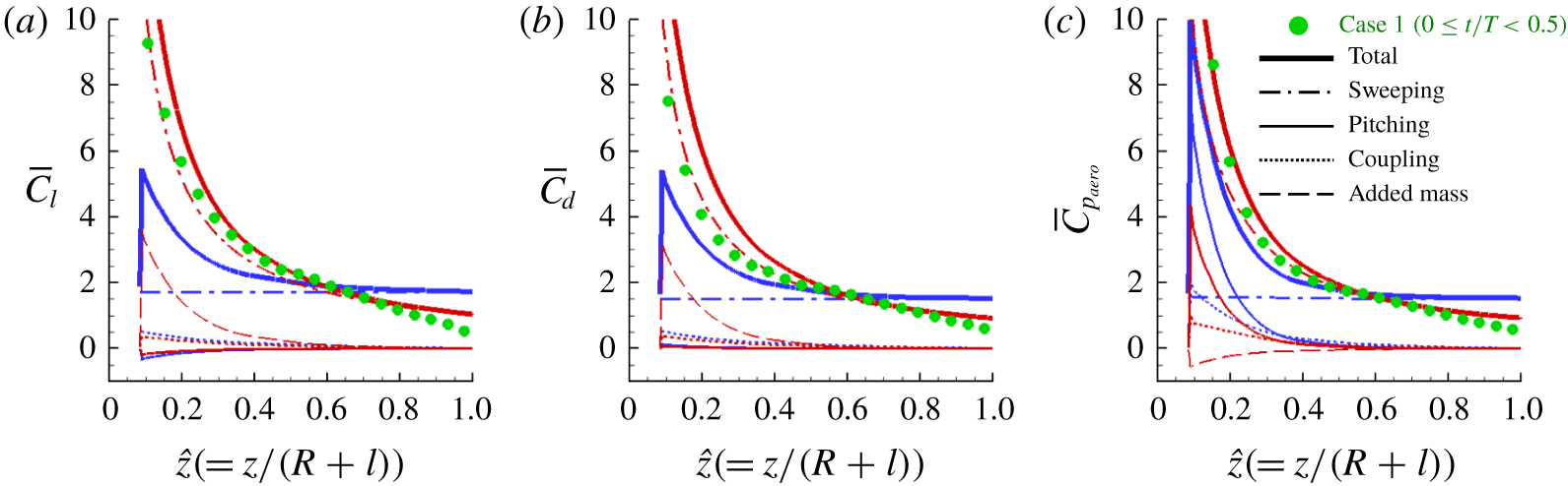
Predicted time-averaged sectional aerodynamic coefficients ( $0\leqslant t/T<0.5$; case 1): (a) lift; (b) drag; (c) aerodynamic power. Red and blue lines denote the results predicted by the present model with
 $w=0$ and model of Wang et al. (Reference Wang, Goosen and van Keulen2016), respectively, and green solid circles are those from the present numerical simulation.

Figure 14 shows the spanwise variations of the time-averaged sectional lift, drag and aerodynamic power coefficients predicted by the present model with  $w=0$ during the first half-stroke, where
 $\overline{C}_{l}=2\,\text{d}\overline{L}/\unicode[STIX]{x1D70C}(z\dot{\unicode[STIX]{x1D719}}_{rms})^{2}c\,\text{d}z$,
 $\overline{C}_{d}=2\,\text{d}\overline{D}/\unicode[STIX]{x1D70C}(z\dot{\unicode[STIX]{x1D719}}_{rms})^{2}c\,\text{d}z$,
 $\overline{C}_{p_{aero}}=2\,\text{d}\overline{P}_{aero}/\unicode[STIX]{x1D70C}(z\dot{\unicode[STIX]{x1D719}}_{crmc})^{3}c\,\text{d}z$, as used in figure 10. Here,
 $\text{d}\overline{L}/\text{d}z$,
 $\text{d}\overline{D}/\text{d}z$ and
 $\text{d}\overline{P}_{aero}/\text{d}z$ can be obtained by the present model together with (5.7) and (5.9). The results from the present numerical simulation and predicted by the model of Wang et al. (Reference Wang, Goosen and van Keulen2016) are also plotted in this figure. The present model quite accurately predicts the sectional force and power coefficients. Since the time-averaged sectional force coefficients due to the wing pitching motion and coupling effects are very small for both models and two models are the same for the added mass effect, the differences in the predicted time-averaged sectional force coefficients mainly come from the sweeping motion. Therefore, the present model for the sectional force coefficients due to the sweeping motion (5.21) seems to be more appropriate. High power coefficients near the wing root are predicted mainly by the sweeping motion in the present model, but they are predicted by the coupling effect and pitching motion in the model of Wang et al. (Reference Wang, Goosen and van Keulen2016).
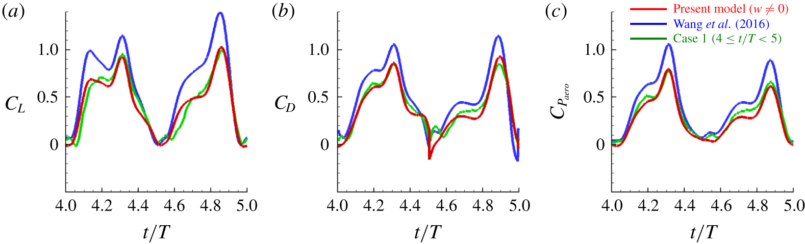
Predicted force and power coefficients using the present model with  $w\neq 0$ and the model of Wang et al. (Reference Wang, Goosen and van Keulen2016), and those from the present numerical simulation during the fifth stroke period (case 1): (a) lift; (b) drag; (c) aerodynamic power.

Figure 15 shows the temporal variations of the lift, drag and aerodynamic power coefficients predicted by the present model with  $w(\neq 0)$ (5.33), together with those from the present numerical simulation (
 $4\leqslant t/T<5$) and predicted by the model of Wang et al. (Reference Wang, Goosen and van Keulen2016). At this time period, the wake behind the hind wing reaches a quasi-periodic state. As shown in this figure, the present model including the effect of the induced downwash motion in the wake accurately predicts the force and power coefficients. The differences between the time-averaged lifts, drags and power consumptions predicted by the present model and from the numerical simulation are 0.5 %, 4.1 % and 10.8 %, respectively, and they may come from the assumptions of steady induced downwash motion (
 $w=w(z)$) and no swirl in the wake. The present result clearly indicates that the inclusion of the downwash motion in the wake (
 $w\neq 0$) is very important in developing an aerodynamic model.
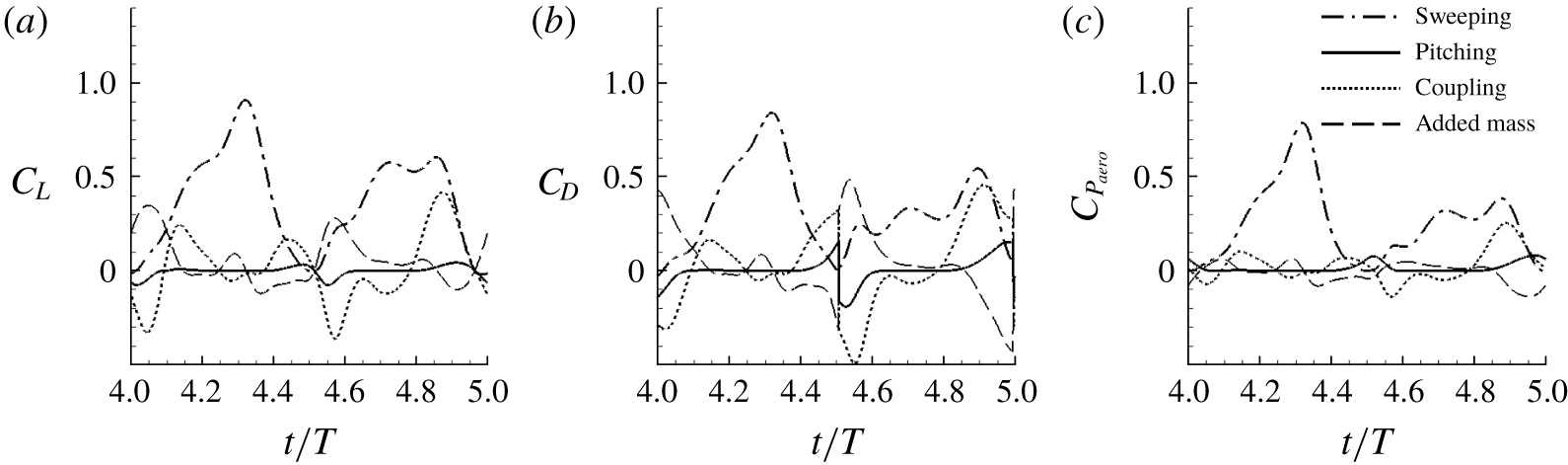
Predicted components of the force and power coefficients using the present model with  $w\neq 0$: (a) lift; (b) drag; (c) aerodynamic power.

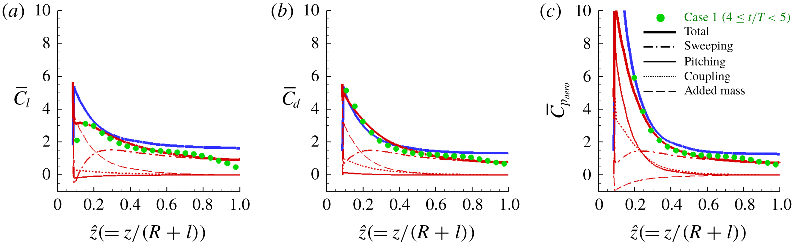
Predicted time-averaged sectional aerodynamic coefficients using the present model with  $w\neq 0$ and the model of Wang et al. (Reference Wang, Goosen and van Keulen2016), and those from the present numerical simulation (
 $4\leqslant t/T\leqslant 5$; case 1): (a) lift; (b) drag; (c) power. Red and blue lines denote the results predicted by the present model (
 $w\neq 0$) and model of Wang et al. (Reference Wang, Goosen and van Keulen2016), respectively, and green solid circles are those from the present numerical simulation.

Figure 16 shows the components of force and the power coefficients predicted by the present model with  $w(\neq 0)$ (5.33). As for the case of the first half-stroke, the sweeping motion is most dominant in generating force and power consumption that are positive during most of the flapping period. The effects of coupling and added mass are also quite large at the start and end of each half-stroke. Due to the coupling effect (5.12), the lift, drag and power become negative at the start of half-stroke (wing pitching down), but positive at the end of half-stroke (wing pitching up). On the contrary, the lift, drag and power due to the added mass effect are positive and negative at the start and end of half-stroke, respectively, because of the wing acceleration and deceleration. The pitching motion hardly produces the force and requires little power except during the stroke reversal. The lift and drag due to the pitching motion are positive before the stroke reversal but negative after that. However, the power due to the pitching motion is positive during the stroke reversal.
Figure 17 shows the spanwise variations of the time-averaged sectional lift, drag and power coefficients predicted by the present model with  $w\neq 0$ and by the model of Wang et al. (Reference Wang, Goosen and van Keulen2016), together with those from the present numerical simulation (
 $4\leqslant t/T<5$). The sectional lift, drag and power coefficients along the spanwise direction predicted by the present model with
 $w\neq 0$ are in good agreement with those from the present numerical simulation. Again, the wing sweeping motion is dominant in generating forces and power consumption away from the wing root (
 $\hat{z}>0.2$), and the added mass and coupling effects are important near the wing root. However, the pitching motion requires non-negligible power near the wing root as much as the coupling term does. Note also that the aerodynamic power consumption due to the added mass is slightly negative. This is from relatively large negative aerodynamic power during the wing deceleration, and thus the hind wing can save a small amount of the aerodynamic power due to the added mass effect.
Fruit fly (D. virilis) wing and its force and power coefficients: (a) wing planform geometry; (b) wing kinematics; (c) lift coefficient; (d) drag coefficient; (e) aerodynamic power coefficient. The results from numerical simulation are from Sun & Tang (Reference Sun and Tang2002).

To investigate the applicability of the present model to other insect wings, we consider a fruit fly (D. virilis) wing that has the Reynolds number ( $Re=253$), aspect ratio (
 $AR=2.4$), sweeping amplitude (
 $\unicode[STIX]{x1D6F7}=150^{\circ }$), non-dimensional radii of the first (
 $\hat{z}_{1}=0.54$) and second (
 $\hat{z}_{2}=0.58$) moments of wing area, and wing planform geometry and kinematics (see figure 18a,b and Sun & Tang (Reference Sun and Tang2002) for the detail), very different from those of the present rhinoceros beetle wing. Figure 18 shows the wing planform of a fruit fly (D. virilis) wing and the force and power coefficients predicted by the present model with (5.33), together with the results from the numerical simulation of Sun & Tang (Reference Sun and Tang2002). The predicted lift, drag and aerodynamic power coefficients are in excellent agreement with those from the numerical simulation by Sun & Tang (Reference Sun and Tang2002). Therefore, the present model may be applied to various wing shapes for their force and power prediction.
Downwash velocity and effective angle of attack (case 1): (a) schematic diagram of the area,  $A_{w}$, for the spatial average of the downwash velocity; (b) temporal and spanwise distribution of the downwash velocity averaged over
 $A_{w}$,
 $\overline{w}^{A_{w}}(t,\hat{z})$, from numerical simulation; (c) spanwise distribution of the downwash velocity averaged over
 $A_{w}$ and
 $t$,
 $\overline{w}^{A_{w},t}(\hat{z})$, from numerical simulation (CFD) and the present model
 $w$ (5.33); (d,e) effective angles of attack at
 $\hat{z}=0.425$ and 0.925, respectively, from numerical simulation and present model.

7 Further consideration on the induced downwash motion
So far, we modelled the induced downwash velocity as steady and non-uniform in the spanwise direction, i.e.  $w(z)$. However, the flow fields behind the wing indicate that the induced downwash motion should be unsteady. Therefore, we consider an unsteady non-uniform downwash motion
 $w(t,z)$ in this section. Figure 19 shows the comparison of the downwash velocities from the present model and numerical simulation for case 1. The area
 $A_{w}$ for the spatial average of the downwash velocity shown in figure 19(a) is similar to those used for computing the effective angle of attack in the previous studies (Birch & Dickinson Reference Birch and Dickinson2003; Kim et al. Reference Kim, Kweon and Choi2015; Han, Nguyen & Han Reference Han, Nguyen and Han2019). As shown in figure 19(b), the downwash velocity
 $\overline{w}^{A_{w}}(t,\hat{z})$ (
 $w(t,\hat{z})$ averaged over
 $A_{w}$;
 $\hat{z}=z/(R+l)$) almost linearly decreases in time except very near the wing tip (
 $\hat{z}\leqslant 0.8$): i.e. it is maximum at the beginning of each half-stroke and minimum at the end of half-stroke, because vortical structures generated in the previous stroke are convected downward. Upward velocity is also observed very near the wing tip due to the tip vortex and just before the stroke reversal because of the leading edge vortex. Figure 19(c) shows the spanwise distribution of the downwash velocity averaged over
 $A_{w}$ and
 $t$ from numerical simulation and the present model
 $w$ (5.33). Except near the wing tip, the predicted downwash velocity
 $w$ is in a good agreement with that from numerical simulation. The discrepancy near the tip comes from the upward induced velocity existing in this region. The effective angles of attack predicted by the present model are compared at two different spanwise locations (near the midspan and tip, respectively) with those obtained from numerical simulation in figure 19(d,e), together with the prescribed angle of attack
 $\unicode[STIX]{x1D6FC}$. Near the midspan (
 $\hat{z}=0.425$),
 $w<\overline{w}^{A_{w}}$ at the early stage of half-stroke and
 $w>\overline{w}^{A_{w}}$ at the late stage because
 $w\approx \overline{w}^{A_{w},t}$ (see figure 19b,c), and thus
 $\unicode[STIX]{x1D6FC}_{e}$ from the present model is larger and smaller than those from numerical simulation at early and late stages, respectively (figure 19d). On the other hand, near the wing tip (
 $\hat{z}=0.925$), the wing velocity is much larger than the induced velocity, so that the effective angles of attack from the present model and numerical simulation are not very different from the prescribed angle of attack (figure 19e).
As shown in figure 19(b), the temporal variation of the downwash velocity may be approximated with a sawtooth profile in time, i.e.  $w(t,z)({\geqslant}0)$, which can be formulated as
 $$\begin{eqnarray}w(t,z)=(1+k)\overline{w}(z)+k\overline{w}(z)f(t),\end{eqnarray}$$
where
 $$\begin{eqnarray}f(t)=\left\{\begin{array}{@{}ll@{}}\displaystyle -\frac{2}{T_{u}}(t-t_{u}) & \text{for }t_{u}\leqslant t\leqslant ~t_{u}+T_{u},\\ \displaystyle -\frac{2}{T-T_{u}}(t-t_{u}-T_{u}) & \text{for }t_{u}+T_{u}\leqslant t\leqslant t_{u}+T_{u}+T_{d},\end{array}\right.\end{eqnarray}$$
 $\overline{w}(z)$ is the downwash velocity averaged over a flapping period,
 $0\leqslant k\leqslant 1$,
 $t_{u}$ is the time corresponding to the upstroke start,
 $T_{u}$ and
 $T_{d}$ are the upstroke and downstroke periods (they not necessarily half of one flapping period (
 $T_{u}+T_{d}$)), respectively. At
 $k=0$,
 $w$ is a steady downwash motion, but
 $w$ becomes a steeper sawtooth wave at a higher
 $k$ (see figure 20a).
A model of the induced downwash velocity and its predictions of the force and power coefficients for different values of  $k$ (case 1): (a)
 $w(t,z)$ (7.1) for
 $k=0$, 0.5 and 1; (b) lift; (c) drag; (d) aerodynamic power. In (b–d), the values of
 $t_{u}/T=3.995$,
 $T_{u}/T=0.511$ and
 $T_{d}/T=0.489$ (
 $k=0$ and 1) are used for (7.1) and (7.2). The results from the present numerical simulation and also from the present model with
 $w=0$ are compared in these figures.

From the momentum theory under the consideration of a periodic downwash motion (Siekmann Reference Siekmann1963; Ellington Reference Ellington1984b), the period-averaged sectional lift of a flapping wing becomes
 $$\begin{eqnarray}\text{d}\overline{L}=2\unicode[STIX]{x1D70C}\unicode[STIX]{x1D6F7}\overline{w^{2}}z\,\text{d}z.\end{eqnarray}$$
For the sawtooth profile of  $w$ in time (7.1),
 $\overline{w^{2}}=\overline{w}^{2}(1+k^{2}/3)$. Therefore, equation (7.3) becomes
 $$\begin{eqnarray}\text{d}\overline{L}=2\unicode[STIX]{x1D70C}\unicode[STIX]{x1D6F7}\overline{w}^{2}\left(1+\frac{k^{2}}{3}\right)z\,\text{d}z.\end{eqnarray}$$
Substituting (7.1) into (5.28) yields
 $$\begin{eqnarray}\text{d}F_{x}^{swp}\sin \unicode[STIX]{x1D702}\approx \text{d}F_{x}^{swp}|_{w=0}\sin \unicode[STIX]{x1D702}+(1+k)\overline{w}I\,\text{d}z+k\overline{w}f(t)I\,\text{d}z.\end{eqnarray}$$
 $$\begin{eqnarray}\text{d}F_{x}^{cpl}\sin \unicode[STIX]{x1D702}\approx \text{d}F_{x}^{cpl}|_{w=0}\sin \unicode[STIX]{x1D702}+(1+k)\overline{w}I^{\prime }\,\text{d}z+k\overline{w}f(t)I^{\prime }\,\text{d}z,\end{eqnarray}$$
where  $I^{\prime }=-\unicode[STIX]{x03C0}\unicode[STIX]{x1D70C}((3/4)c-d)c\dot{\unicode[STIX]{x1D702}}\sin \unicode[STIX]{x1D702}\cos \unicode[STIX]{x1D702}$. Substituting (7.5) and (7.6) into (5.24) with
 $\overline{I^{\prime }}=0$ gives
 $$\begin{eqnarray}\text{d}\overline{L}\approx \overline{w}[(1+k)\overline{I}+k\overline{fI}+k\overline{fI^{\prime }}]\,\text{d}z+\text{d}\overline{L}|_{w=0}.\end{eqnarray}$$
Equating (7.4) with (7.7) provides a quadratic equation for  $\overline{w}$,
 $$\begin{eqnarray}2\unicode[STIX]{x1D70C}\unicode[STIX]{x1D6F7}\overline{w}^{2}\left(1+\frac{k^{2}}{3}\right)z=\overline{w}\underbrace{[(1+k)\overline{I}+k\overline{fI}+k\overline{fI^{\prime }}]}_{\equiv \;\overline{I}^{\ast }}+\frac{\text{d}\overline{L}|_{w=0}}{\text{d}z}.\end{eqnarray}$$
If  $\overline{I}^{\ast }$ is negative and the last term in (7.8) is positive,
 $\overline{w}$ is obtained by
 $$\begin{eqnarray}\overline{w}=\frac{1}{4\unicode[STIX]{x1D70C}\unicode[STIX]{x1D6F7}z(1+k^{2}/3)}\left\{\overline{I}^{\ast }+\left[{\overline{I}^{\ast }}^{2}+8\unicode[STIX]{x1D70C}\unicode[STIX]{x1D6F7}z\left(1+\frac{k^{2}}{3}\right)\frac{\text{d}\overline{L}|_{w=0}}{\text{d}z}\right]^{1/2}\right\}\geqslant 0\quad \text{for }z\neq 0.\end{eqnarray}$$
Here,  $\overline{I}^{\ast }=\overline{I}$ when
 $k=0$, and thus (7.9) is reduced to (5.33).
To examine the effect of the unsteadiness of the downwash motion in the present model, we obtain the aerodynamic force and power coefficients predicted by the present model ((5.10)–(5.13), (5.21) and (5.22)) together with (7.1), (7.2) and (7.9) for  $k=0$ and 1, respectively, and compare the results with those from the present numerical simulation (case 1) and also from the present model with
 $w=0$ in figure 20(b–d). As shown, the predicted results from the present model with non-zero
 $w$ (with
 $k=0$ and 1) agree very well with those of the numerical simulation, indicating that the unsteadiness of
 $w$ in the model is not very important in predicting the aerodynamic performance at least for the present wing kinematics and geometry being considered. Note also that the model with
 $w=0$ (i.e. no induced downwash motion) does not accurately predict the aerodynamic forces.
8 Conclusions
In the present study, the aerodynamic force generated and power required by hovering motion of a rhinoceros beetle (Trypoxylus dichotomus) were investigated using numerical simulations, and a quasi-steady blade element theory combined with a momentum theory was suggested to predict the force and power on the wing. The wing kinematics of a hovering beetle were measured using three high-speed cameras, and the geometries of body and elytron were three-dimensionally scanned for the use of numerical simulation. We showed from numerical simulation that the twist of the hind wing along the wing span direction has a positive but marginal effect on the total force and power on the wing, and the aerodynamic role of the elytron is negligible in producing the lift and drag forces. Thus, the hind wing alone can generate the vertical force enough to support the weight. The elytron may play a role when it moves forward or turns during flight (see, for example, Le et al. (Reference Le, Truong, Park, Truong, Ko, Park and Byun2013)). However, its detailed mechanism may be further investigated to fully understand its aerodynamic function.
We developed a predictive quasi-steady blade element theory for the force produced and power required by hovering motion, in which the effects of the wing–wake interaction as well as the wing sweeping, pitching, their coupling and added mass were included. For the wing–wake interaction, the wake generated by a flapping wing was modelled as a steady or unsteady non-uniform induced downwash motion, and this downwash motion was derived by combining the blade element theory with the inviscid momentum theory. Both models with steady and unsteady induced downwash motions provided excellent agreement with the numerical results, indicating that the steady downwash motion alone should be enough to provide accurate force generation and power consumption. With the aerodynamic model developed, we showed that the wing sweeping motion mainly contributes to aerodynamic force generation and power consumption. The added mass and coupling of sweeping and pitching motions were also important contributors to the force production and power consumption. The pitching motion hardly generated the aerodynamic forces but required the aerodynamic power near the wing root. The present aerodynamic model with the steady non-uniform induced downwash motion is a predictive model since it does not include any model constants, and thus may be used for various wing geometries. Therefore, the present model may be used for the optimizations of the flapping-wing geometry and kinematics to enhance the performance of the flapping wing in hover.
Finally, we would like to mention the limitations of the present model. First, as mentioned by Wang et al. (Reference Wang, Goosen and van Keulen2016), the present model assumed a quasi-steady state at each instant of the wing motion and thus neglected the Wagner effect (Wagner Reference Wagner1925). However, as indicated by Wang et al. (Reference Wang, Goosen and van Keulen2016), the Wagner effect may be small at high angles of attack and low Reynolds numbers. Second, the present model was based on the model equations for the drag and lift coefficients ((5.16) and (5.20)) that were tested for the ranges of  $2.83\leqslant AR\leqslant 3.74$ and
 $136\leqslant Re\leqslant 8071$ (see Oh & Choi Reference Oh and Choi2018). Thus, the present model may provide poor predictions for a much wider range of these parameters. However, since many insect wings operate at these parameter ranges (Lentink & Dickinson Reference Lentink and Dickinson2009), the present model may be predictive for most hovering insect wings. Third, we developed our model for a wing without camber. Therefore, a further study is required to develop a model for a flapping wing with camber in the future.
Measurement of the wing and body motions of a hovering rhinoceros beetle: (a) experimental set-up; (b) distribution of morphological markers; (c) body displacement. In (b), white, red and yellow circles indicate tracking points on the body (1: mouth; 2: mass centre; 3: pygidium), right elytron (1: shoulder; 2: leading edge at midspan; 3: trailing edge at midspan; 4: wing tip) and hind wing (1: shoulder; 2–5: leading edges at  $r_{h}=0.1R_{h}$,
 $0.3R_{h}$,
 $0.6R_{h}$ and
 $0.9R_{h}$; 6–9: trailing edges at
 $r_{h}=0.1R_{h}$,
 $0.3R_{h}$,
 $0.6R_{h}$ and
 $0.9R_{h}$; 10: wing tip), respectively. Linear regression lines are also plotted in (c).

Acknowledgements
This research was supported by a grant to the Bio-Mimetic Robot Research Center funded by the Defense Acquisition Program Administration and by the Agency for Defense Development (UD160027ID), as well as by the research program (NRF-2016R1E1A1A02921549, 2017R1A4A1015523 and 2019R1A2C2086237) of the Ministry of Science and ICT of Korea.
Declaration of interests
The authors report no conflict of interest.
Supplementary materials
Supplementary materials are available at https://doi.org/10.1017/jfm.2019.962.
Appendix A. Measurement of the wing kinematics
Experimental arrangements are the same as those of Lee et al. (Reference Lee, Park and Kim2015a). A hovering flight of a Trypoxylus dichotomus is filmed in a customized studio frame  $(2~\text{m}\times 2~\text{m}\times 2~\text{m})$ with three high-speed cameras (NX5-S2 MONO, Integrated Design Tools, Inc.) having maximum spatial resolution of
 $2336\times 1728$ pixels at maximum sampling rate of 730 fps, as shown in figure 21(a). One camera is located on the top and the others are located at the sides of the frame. Also, two 2 kW-halogen portable lights are used for illumination. These cameras capture the images during two seconds at the rate of 2000 fps with a spatial resolution of
 $512\times 512$ pixels and operate simultaneously via a synchronizer (miniHUB, Integrated Design Tools, Inc.). The sequential image analysis is used to separate captured images of the hovering beetle during two consecutive periods. We use seventeen soft markers that are morphologically discernible features to let the beetle fly without any external disturbance instead of using hard markers. Figure 21(b) shows selected markers including three on the body, four on the right elytron and ten on the right hind wing. The cross-correlation of pixels is performed across the acquired image sequences, known as visual image correlation method, to track the soft markers (Hedrick Reference Hedrick2008). With the visual image correlation method, we use modified direct linear transform (known as MDLT) algorithm for the reconstruction of three-dimensional wing kinematics (Hatze Reference Hatze1988; Hedrick Reference Hedrick2008).
Figure 21(c) shows the measured body displacement in  $X$- and
 $Y$-directions, where
 $X$- and
 $Y$-directions indicate the frontal and anti-gravitational directions, respectively. Also, linear regression lines are plotted to roughly estimate the mean velocity for both directions. With the least square method, the mean velocity is 0.14 and
 $-0.05~\text{m}~\text{s}^{-1}$ in
 $X$- and
 $Y$-directions, respectively. The advance ratio
 $J$ is defined as the ratio of the forward velocity to the mean velocity of wing tip
 $U_{h}=2\unicode[STIX]{x1D6F7}_{h}\,fR_{h}$ (Ellington Reference Ellington1984a), and the flight of
 $J<0.1$ is regarded as a hovering flight. From the measured data,
 $J\approx 0.01$ and the motion in the vertical direction is much slower than that in the frontal direction. Thus, it is reasonable to assume that the present wing motions measured are indeed those of the hovering beetle.