





1. Introduction
In 2015, the ice shelves of northern Ellesmere Island covered 535 km2, approximately half of their area at the start of the 21st century (Mueller and others, Reference Mueller, Copland, Jeffries, Copland and Mueller2017a). Some ice shelves have been lost completely in recent decades, such as the Ayles in 2005 (Copland and others, Reference Copland, Mueller and Weir2007) and the Markham in 2008 (Mueller and others, Reference Mueller, Copland, Jeffries, Copland and Mueller2017a), while others have lost significant area, such as the Petersen (31.0 km2 loss, 61.6%, 2003–12; White and others, Reference White, Copland, Mueller and Van Wychen2015) and the Serson (187.1 km2 loss, 95.5%, 2003–15; Mueller and others, Reference Mueller, Copland, Jeffries, Copland and Mueller2017a). These losses have resulted in ice-free fiords for the first time in ∼3500–5500 years (England and others, Reference England, Evans, Lakeman, Copland and Mueller2017) and have occurred in tandem with a period of rapidly rising air temperatures and significant reductions in the age and thickness of sea ice fringing northern Ellesmere Island (Kwok, Reference Kwok2018; Meier and Stroeve, Reference Meier and Stroeve2022). Despite the extensive fracturing that was apparent across the Milne Ice Shelf (Fig. 1), it remained relatively stable compared to the other ice shelves on northern Ellesmere Island during this period, reducing in area from 200.6 km2 in 1998 to 187.4 km2 in 2015, a loss of only 6.6% (Mueller and others, Reference Mueller, Copland, Jeffries, Copland and Mueller2017a). However, in late July 2020, a massive calving event resulted in the loss of 43% of the Milne Ice Shelf (Fig. 1c), including a 79 km2 fragment that soon fractured into two large pieces, which then drifted westward in the Arctic Ocean (Vincent and Mueller, Reference Vincent and Mueller2020).
Study site maps. (a) The Milne Ice Shelf showing the location of each mass balance site (blue and red circles), automatic weather station (AWS, triangles) at Purple Valley (PV, black), M5 (blue), M3 (green) and M1 (red). The ice shelf Outer, Central and Inner units first described by Jeffries (Reference Jeffries1986b) are shown along with the Milne Glacier ice tongue to the south. The approximate boundary between the Outer and Central units is shown with a curved dotted line. The gradient from the seaward to the landward edge of the ice shelf is shown with a black dashed line. The M1 stake and AWS drifted ∼1 km south in August 2012 (both original and new positions shown). Base image: Landsat-8, 23 July 2018. (b) Location of the study area (in red box) in the Queen Elizabeth Islands is shown, along with Ellesmere Island ice shelves and ice shelf remnants as of 2015 (Mueller and others, Reference Mueller, Copland and Jeffries2017b). Glaciated areas are from the Randolph Glacier Inventory (RGI) version 7. (c) The Milne Ice Shelf following calving of 43% of its area in 2020, with its 2015 extent for comparison (Mueller and others, Reference Mueller, Copland and Jeffries2017b). Base image: Planet Labs, 11 August 2020.

1 Long description
A) Map of the Milne Ice Shelf showing mass balance sites with red circles for Central Unit stakes and blue circles for Outer Unit stakes. Automatic weather stations (AWS) are marked with triangles: PV-AWS (yellow), M1-AWS (red), M3-AWS (orange), M5-AWS (blue). The map includes Cape Egerton, Cape Evans, Glacier 1 to Glacier 6 and Epishelf Lake. The seaward and landward edges are marked with dashed lines. B) Map of the Queen Elizabeth Islands showing the location of the study area in a red box, with ice shelves, glaciers and land areas marked. Key locations include Milne Fiord, Ward Hunt Ice Shelf, Axel Heiberg Island and Ellesmere Island. C) Detailed map of the Milne Ice Shelf with mass balance sites marked as in A, showing the boundary of the study area with pink lines. Coordinates range from 82.0°N to 82.8°N and 81.0°W to 82.0°W.
Based on previous observations, the Milne Ice Shelf appeared to be unique among the other northern Ellesmere ice shelves for its structural stability (Mueller and others, Reference Mueller, Copland, Jeffries, Copland and Mueller2017a). Some have suggested that the lack of calving events, aside from a major calving event from its seaward coastline in the 1960s and a 3 km2 loss in 2012/13 (near Cape Evans; Mueller and others, Reference Mueller, Copland, Jeffries, Copland and Mueller2017a), could be linked to the supportive physiography of Milne Fiord (Jeffries, Reference Jeffries1986a; Veillette and others, Reference Veillette, Mueller, Antoniades and Vincent2008). However, little is currently known about the surface mass balance of the ice shelf, its spatial and temporal variability and the factors that control it. This limits understanding of the causes of the 2020 calving event, including the impact of thinning reported by Mortimer and others (Reference Mortimer, Copland and Mueller2012), the roles of basal vs surface melt and how the ice shelf may evolve in the future.
This study evaluates the hypothesis that a surface mass balance gradient occurs along the inland-to-ocean length of the Milne Ice Shelf due to variations in microclimate. Accordingly, we combine field measurements and remote sensing to examine surface accumulation and ablation patterns, identify the factors controlling surface mass balance processes and evaluate how these processes have varied over time during a period of climate warming. An understanding of these processes may provide insight into the stability of the remaining ice shelves on Ellesmere Island and in other coastal regions with a semi-permanent floating ice cover (e.g. multi-year landfast sea ice [MLSI], ice tongues and tidewater glaciers).
2. Study area
The Milne Ice Shelf is located in Milne Fiord (82°41′ N, 81°25′ W), situated on the northern coast of Ellesmere Island, approximately ∼275 km west of Alert and ∼310 km north of Eureka (Fig. 1b). Milne Fiord is approximately 436 m deep and extends ∼40 km from the Milne Glacier grounding line to its head, widening from ∼6 km inland to ∼16 km where the ice shelf met the Arctic Ocean prior to the 2020 calving event (Hamilton and others, Reference Hamilton, Mueller and Laval2021). After the Ward Hunt Ice Shelf, the Milne Ice Shelf has been the second largest of the remaining Canadian ice shelves since the start of the 21st century, measuring 187.4 km2 in March 2015 (Mueller and others, Reference Mueller, Copland, Jeffries, Copland and Mueller2017a), but this was reduced by 80.9 km2 to make a total area of 106.5 km2 in July 2020. The surface of the ice shelf is characterized by surface undulations or rolls that consist of a series of ridges separated by melt-pond-filled troughs (Hattersley-Smith, Reference Hattersley-Smith1957; Coffey and others, Reference Coffey2022). Jeffries (Reference Jeffries1986a) divided the ice shelf into individual units based upon the differing geometry of the undulating surface topography. The rolls across the Outer Unit are oriented parallel to the coastline (i.e. southwest to northeast) with a longer wavelength (∼300 m) and become increasingly disorganized and shorter towards the Central Unit (∼150–180 m; Fig. 1a). The Inner Unit described by Jeffries (Reference Jeffries1986a) is now recognized as an epishelf lake, composed of a layer of buoyant freshwater overlying sea water, developed from summer melt of snow and glacier ice that is dammed by the ice shelf (Veillette and others, Reference Veillette, Mueller, Antoniades and Vincent2008; Bonneau and others, Reference Bonneau, Laval, Mueller, Hamilton, Friedrichs and Forrest2021). Jeffries (Reference Jeffries1986a) associated the variation in surface topography with ice thickness variations derived by Prager (Reference Prager1983); the more developed ridges occurred in the Outer Unit where thicker ice (up to 90 m) was more widespread. Ground-penetrating radar (GPR) measurements in 2008/09 by Mortimer and others (Reference Mortimer, Copland and Mueller2012) showed that the ice shelf had a mean thickness of 55 ± 1.1 m, with the thickest ice (70–80 m) located across the Outer Unit and considerably thinner ice (∼50 m) in the Central Unit, except where glacier inflow produced localized thickening of up to 94 m (fig. 1c in Mortimer and others, Reference Mortimer, Copland and Mueller2012).
The first accurate measurement of the area of the Milne Ice Shelf is from 1959, when aerial photos indicated an extent of 287.6 km2 (Jeffries, Reference Jeffries1986b; Mueller and others, Reference Mueller, Copland, Jeffries, Copland and Mueller2017a). For the remainder of the 20th century, the only significant loss from the northern (front, seaward) edge of the ice shelf occurred between 1959 and 1963, when 27 km2 broke away. However, this area was replaced by MLSI, named the Milne Re-entrant, which thickened in situ to reach a thickness of 7.24–9.80 m by spring 1985 (Jeffries, Reference Jeffries1986b). The Milne Re-entrant remained in place until February 1988, when it detached from the ice shelf as a large MLSI floe during a brief episode of strong offshore winds (Jeffries, Reference Jeffries1992, Reference Jeffries, Williams and Ferrigno2002). With the exception of a minor calving event in 2012/13 and the major event in 2020, all area losses since 1963 have occurred along the southern (rear, landward) edge of the ice shelf, where the ice shelf ice has been replaced by an epishelf lake ice (for a detailed list of Milne Ice Shelf area changes, see table 4 in Mueller and others, Reference Mueller, Copland, Jeffries, Copland and Mueller2017a). This epishelf lake ice has thinned from a maximum of 3.19 m in 1983 (Jeffries, Reference Jeffries1985) to ∼1.5 m in summer 2018 and 2019 (D. Mueller, unpublished data). Mortimer and others (Reference Mortimer, Copland and Mueller2012) compared terrestrial GPR measurements collected in 2008 and 2009 with airborne radio-echo sounding measurements collected in 1981 to determine that mean ice shelf thickness decreased by ∼13 m over this period. The measurements revealed spatial variability in the thinning rate, with a higher rate of loss from the landward Central Unit compared to the seaward Outer Unit (fig. 4c of Mortimer and others, Reference Mortimer, Copland and Mueller2012).
Richer-McCallum (Reference Richer-McCallum2015) examined shallow ice cores (∼2 m long) from both the Central and Outer units of the Milne Ice Shelf to identify their ice source based on salinity and structural characteristics (i.e. bubble shape, size and density). This study confirmed that meteoric ice (i.e. originating from atmospheric precipitation; Jeffries, Reference Jeffries, Copland and Mueller2017) was present across the Outer Unit, while meteoric ice and old sea ice were identified across the Central Unit. Although past studies described the Milne Ice Shelf as having originated from glacier ice (Jeffries, Reference Jeffries1986a), the results presented by Richer-McCallum (Reference Richer-McCallum2015) suggest that it is more likely a composite-type, being composed of both sea ice and glacier ice (Lemmen and others, Reference Lemmen, Evans and England1988). Composite ice shelves can accumulate mass via glacier inflow, surface snowfall, basal freeze-on and sea ice accretion, while ablation occurs via surface runoff, basal melt and calving (Dowdeswell and Jeffries, Reference Jeffries, Copland and Mueller2017). Although five tributary glaciers currently terminate along the sides of the Milne Ice Shelf, glacial input has been limited to Glacier 2 since 2011 (Mortimer and others, Reference Mortimer, Copland and Mueller2012) (Fig. 1a).
3. Methods
3.1. Mass balance
The surface mass balance of the Milne Ice Shelf was measured from a network of eight ablation stakes established in early April 2008, spanning the ice shelf length and width (Fig. 1a). Sites M5, M4, M8 and M9 were situated in the Outer Unit, while sites M1, M2, M3 and M7 were placed in the Central Unit. In August 2012, the epishelf lake lost some of its ice cover, and M1 became detached from the ice shelf and drifted south by 1.2 km on a small (∼120 m-long) ice fragment. Mass balance measurements were made annually between 2008 and 2018, except in 2010; complete annual mass balance data are available for 2009 and 2012–19, while the 2011 mass balance represents the combined change over 2010/11 (Supplementary Table S1). The entire network of eight ablation stakes could not always be visited every field season due to logistical constraints, but a minimum of four sites were measured during each field season. At each visit, the stake height above the ice and the snow depth were measured, and a new stake was installed if the previous stake was near to melting out. The locations of the ablation stakes were recorded using a Global Navigation Satellite System (GNSS) receiver.
During spring field seasons in April to May 2008, 2011 and 2013, the densities of snow layers were measured in snow pits at each site. The depth-integrated density for the snowpack was used to determine snow water equivalent (SWE) at every site. The coefficient of variation for these 3 years (n = 6, 8 and 5) never exceeded 43%. In 2009, density measurements were limited to one snow pit, so the depth-averaged density from the snow pit was used to determine SWE at sites without a snow pit that year, with an assumed error of 43%. In 2012 and 2014–19, the study sites were visited in summer (28 June to 24 July), when only two snow pits were sampled, yielding a mean density of 569 kg m−3. This value, with an assumed error of 43%, was applied to all sites where snow remained but densities were not measured.
Specific annual surface mass balance was calculated for each stake using the floating-date system (Cogley and others, Reference Cogley2011). In this convention, the annual balance represents the difference in snow and ice mass at the ice surface between site visits. The water equivalent of the ice gained (positive) or lost (negative), using a density of 880 kg m−3 with uncertainty of ±16 kg m−3 based on shallow ice core measurements (see Section 3.4 for details), was added to the SWE gained/lost between successive visits to yield a surface mass balance value. The midpoint of the field season (field season duration ranged from 1 to 10 days) was used to calculate the time elapsed between quasi-annual measurements. Except for mass balance year 2011, all stakes that were not visited annually were removed from the analysis. When there was more than one ablation stake measurement at a site, the mass balance and SWE measurements at all stakes (up to n = 3) at the site were averaged, and uncertainty was added in quadrature with the standard error of the mean (SEM) of these values.
Mass balance for all sites across the Outer and Central units was computed as the mean mass balance. Uncertainty was propagated as above, and the SEM was computed when n > 1. A final aggregation to the entire ice shelf was conducted by combining the values and uncertainty from the two units in proportion to their respective areas (65% of total ice shelf area for the Outer Unit and 35% for the Central Unit).
3.2. Microclimatology
To examine the climate and its link to surface mass balance across the ∼20 km length of the Milne Ice Shelf, three automated weather stations (AWS; M1-AWS, M3-AWS and M5-AWS, from inland to ocean, respectively; Fig. 1a) were installed on the ice shelf surface in June 2012. Climate conditions further inland were observed using data from an additional AWS located in Purple Valley (PV-AWS; Copland and Mueller, Reference Copland and Mueller2021), located ∼1 km from the Milne Glacier tongue, which was installed in May 2009. The stations contained sensors to record incoming shortwave radiation (Hobo Silicon Pyranometer Smart Sensor S-LIB-M003), air temperature and relative humidity (Hobo 12-bit temperature/RH sensor S-THB-M00X) and height to the snow/ice surface using a sonic ranger (Senix ToughSonic TS-15S at PV-AWS). PV-AWS recorded air temperature at two sensors installed 1 and 2 m above the surface, with the mean of these values used in this study.
Data from each AWS were carefully inspected, and suspected erroneous values were removed. This included filtering for unreasonable values (e.g. temperatures <−60°C) and removing data when the stations fell over. The tilt of M3-AWS affected the incoming shortwave radiation data from August 2012 to May 2013, and the pyranometer on M1-AWS suddenly gave values that were ∼20% less than previous data after July 2014, so these values were removed. A 13 hour running median filter was applied to the sonic ranger data at PV-AWS to reduce noise.
All AWS data were gap-filled using a spline interpolation for outages of up to 11 hours for all stations, and daily averages were computed for each site. M1-AWS and M3-AWS recorded almost continuously from June 2012 to December 2017 (Supplementary Figure S1). M5-AWS only recorded from June 2012 to August 2013 due to an instrumentation failure after water damage. PV-AWS recorded almost continuously between 2009 and 2019.
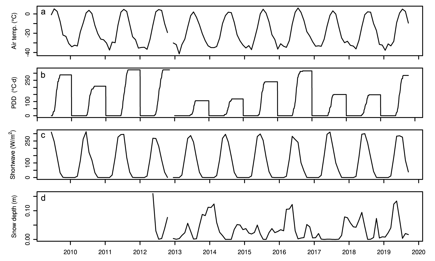
PV-AWS was used as an index station to examine how climatological factors (e.g. air temperature) influence regional surface mass balance because it provides the longest and most continuous meteorological record available (Supplementary Figure S1) and should capture the interannual variability at M1, M3 and M5 on the ice shelf (Fig. 2). The cumulative total of daily above-freezing mean temperatures, known as positive degree-days (PDD; °C·d), was calculated between site visits. The cumulative total of daily below-freezing mean temperatures, or negative degree-days (NDD; °C·d), was also tabulated along with the cumulative total of mean daily incoming shortwave radiation (CSR; J m−2). The PV-AWS cumulative snowfall was calculated as well from the sum of daily positive changes in snow depth.
Climate at PV-AWS (May 2009 to July 2019). (a) Mean monthly air temperature (°C). (b) Annual cumulative positive degree-days (PDD; °C·d). (c) Incoming shortwave radiation (W m−2). (d) Mean monthly snow depth (m).

Figure 2 Long description
Line graph with the y-axis label Air temp. (C) and tick labels 0, minus 20, minus 40. The x-axis shows years from 2010 to 2020. The line forms repeating peaks near 0 and troughs between minus 20 and minus 40 across the full time span. Line graph with the y-axis label PDD (C d) and tick labels 0, 100, 250. The x-axis shows years from 2010 to 2020. The line shows repeated step-like rises from near 0 up to around 250, followed by returns to near 0, repeating across multiple years. Line graph with the y-axis label Shortwave (W m superscript minus 2) and tick labels 0, 100, 250. The x-axis shows years from 2010 to 2020. The line shows repeated peaks near 250 and low values near 0, repeating across the full time span. Line graph with the y-axis label Snow depth (m) and tick labels 0.00 and 0.10. The x-axis shows years from 2010 to 2020. The line is near 0.00 for extended periods and rises in multiple intervals, with several peaks above 0.10, including a prominent peak near 2019.
3.3. Spatial gradient analysis
To assess the relationship between surface mass balance and distance from the ice shelf front (northern, seaward edge), we used a linear mixed effects model, which accounted for the pseudo-replication inherent in revisiting the sites annually (Pinheiro and Bates, Reference Pinheiro and Bates2000; Crawley, Reference Crawley2007). The model predicts surface mass balance using the distance from the northern edge as an independent variable (fixed effect), while accounting for environmental conditions between site visits (random effect). The model is, therefore, comprised of a slope and intercept to reveal the overall gradient in surface mass balance along the length of the Milne Ice Shelf, while also fitting parameters that are unique to each of the ten intervals between site visits. Since PDD, NDD and incoming shortwave radiation data are available for all but the first surface mass balance year (2008/09), these (n = 9 random effects groups) were used instead of balance year to define the groups. Each of these three models explained the same amount of variance in surface mass balance and differed only in the slope and intercept that were fit to account for the random effect associated with the environmental conditions during each balance year. Another version of the model was fit with cumulative snowfall as a random effect, which represented eight balance years (and is not directly comparable to the nominal model).
The final form of the model described above was produced using the lme4 package in R (version 1.1-37; Bates and others, Reference Bates, Mächler, Bolker and Walker2015) and was determined using both forward selection (from a null model) and backward selection (from a saturated model), with fit determined using maximum-likelihood and model parsimony and skill determined using the Akaike information criterion. Models were compared using analysis of variance to arrive at the optimal model, which was recalculated using restricted maximum-likelihood estimates (Bates and others, Reference Bates, Mächler, Bolker and Walker2015). The distribution of model residuals was visually inspected for patterns and to assess homoscedasticity, and normality was assessed using a Shapiro–Wilk test (Crawley, Reference Crawley2007). The variance explained by the model was calculated using Nakagawa’s formula from the performance package in R (Lüdecke and others, Reference Lüdecke, Ben-shachar, Patil, Waggoner and Makowski2021). The 95% confidence interval of the fixed effect was used to evaluate the significance of the model, while leave-one-out cross-validation (by individual site and by random effects group) was used to examine its robustness.
3.4. Distribution of ice facies
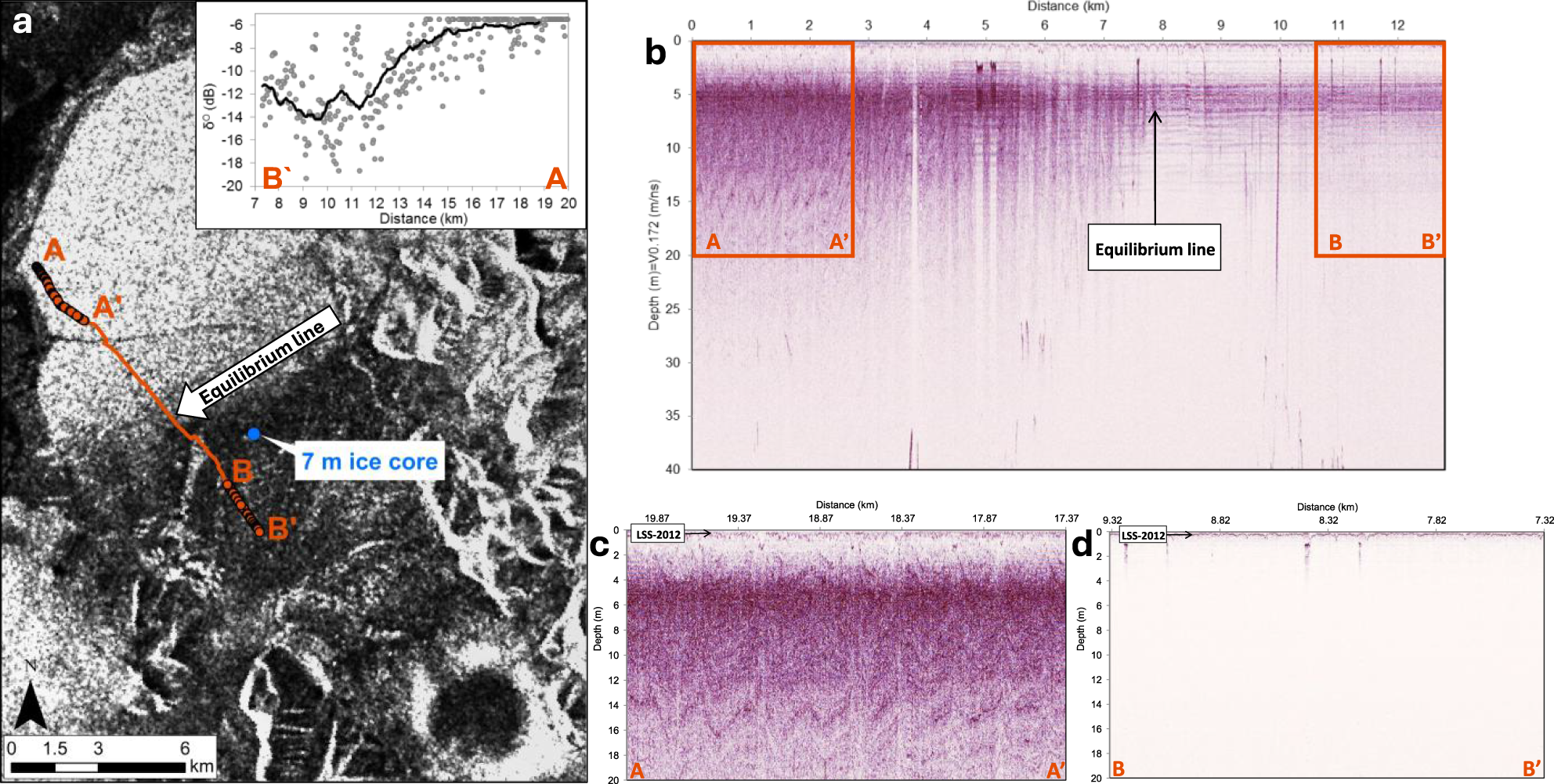
To examine the spatial distribution of ice facies, a GPR transect was collected in May 2013 to examine near-surface characteristics of the ice shelf. Data were collected with a Sensors and Software PulseEKKO Pro GPR system with 500 MHz dipole antennas. The antennas were mounted in a plastic sled and towed behind a snowmobile in a transect along the Milne Ice Shelf at a speed of ∼10 km h−1. Positioning was provided with a built-in single-frequency GNSS receiver that recorded the location of each GPR trace to an accuracy of ∼5 m. Traces were sampled at a temporal resolution of 0.2 ns over a total time window of 1000 ns, stacked eight times and recorded every 0.2 s along the transects. The GPR transect extends from the northern margin of the Outer Unit (seaward edge) to the southern part of the Central Unit (landward edge) to determine any spatial variability in subsurface layering (Fig. 3a). The GPR data were processed in EKKO_Project Version 4 using a signal saturation correction (‘dewow’), frequency filtering (vertical bandpass) and radar gain adjustments (spreading and exponential calibrated compensation). Duplicate traces, generated when the snowmobile was stationary, were deleted.
(a) Location of the 500 MHz GPR transect collected in May 2013 across the Milne Ice Shelf (base image: Radarsat-2 ScanSAR wide, HH, 26 March 2013, 21:31:19); (b) ∼13 km long transect (A to B′) spanning from the Outer Unit to the Central Unit; (c) 2.68 km long transect (A to A′) along the Outer Unit that shows strong sub-surface layering, including the last summer surface from 2012 (LSS-2012); (d) 2.01 km long transect (B to B′) along the Central Unit of the Milne Ice Shelf. Approximate position of the equilibrium line (a, b) is indicated where sub-surface layering reaches the surface. Inset graph (a): backscatter values (σ0) with a 35 m running average, extracted from the SAR image along the GPR transect. Horizontal axis represents distance from the rear of the ice shelf.

Figure 3 Long description
The scientific figure consists of four panels labeled a, b, c and d. Panel a is a satellite basemap with overlaid transects labeled A to A′ and B to B′, showing the equilibrium line and a 7 m ice core location. An inset graph displays backscatter values (sigma) against distance in kilometers, with sigma representing radar backscatter intensity. The horizontal axis is labeled distance in kilometers, ranging from 7 to 20. Panel b is a GPR radargram showing amplitude versus distance and depth, with the vertical axis labeled depth in m multiplied by 10 superscript 3 ns, ranging from 0 to 40 and the horizontal axis labeled distance in kilometers, ranging from 0 to 12. The equilibrium line is marked between A′ and B′. Panel c is a radargram from A to A′, showing depth in meters and distance in kilometers, ranging from 18.87 to 19.87, indicating strong sub-surface layering including the last summer surface from 2012 (LSS-2012). Panel d is a radargram from B to B′, showing depth in meters and distance in kilometers, ranging from 7.32 to 8.32, with less pronounced layering compared to panel c. The main scientific takeaway is the change in sub-surface layering across the equilibrium line, with stronger reflections and continuity observed in panel c compared to panel d.
To interpret and validate the GPR radargrams, a 7 m ice core was extracted at M1 (Fig. 1a) in May 2013, using a Kovacs Mark II ice coring system. Upon extraction, each ice core segment was measured lengthwise, photographed, cut into sections with an ice saw and weighed. A visual examination of stratigraphy was made to assess each core segment for the presence of features characteristic of different facies, such as firn or ice layers. The radio-wave velocity (RWV) was calculated using the mean density of four 2 m ice cores at M3, M4, M5 and M8 nearest the GPR transect using the methods described by Kovacs and others (Reference Kovacs, Gow and Morey1995). Measured densities ranged from 864 to 896 kg m−3, equating to a RWV ranging from 0.171 (M3; Central Unit) to 0.173 m ns−1 (M5; Outer Unit), respectively. This compares closely to a RWV of 0.170 m ns−1 determined by Mortimer and others (Reference Mortimer, Copland and Mueller2012) from a common midpoint survey on Milne Fiord epishelf lake in May 2009.
To assess temporal and spatial variations in ice facies across the ice shelf, backscatter properties in synthetic aperture radar (SAR) satellite imagery were analysed. European Remote-Sensing Satellite-1 (ERS-1), RADARSAT-1 and RADARSAT-2 images acquired in winter and early spring (to avoid any influence from surface melt) provided data from 1992 to 2018 (Supplementary Table S2). To examine the variation in SAR backscatter in the Outer and Central units in relation to the GPR measurements, a RADARSAT-2 image from winter 2013 was radiometrically corrected to a normalized radar cross-section (σ0) in a linear power scale. A low-pass 3 × 3 averaging filter was applied over each raster cell to smooth the image and minimize speckle in ArcGIS Desktop 10.6. Backscatter values were extracted along a 13 km transect from the northern margin (seaward edge) of the Outer Unit to the southern margin (inland edge) of the Central Unit and compared to σ0 values from SAR scenes acquired in 1992, 1998, 2006, 2013 and 2018 to assess temporal changes.
4. Results
4.1. Surface mass balance
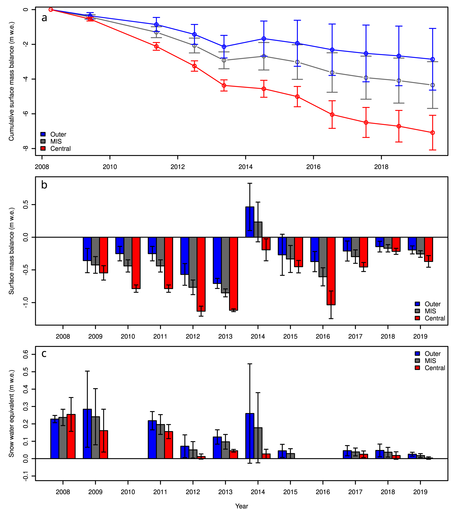
For the 11 year period from 2009 to 2019, the mean annual surface mass balance of the Milne Ice Shelf was −0.40 ± 0.13 m water equivalent (m w.e.). Over this period, winter snow accumulation remained low (Supplementary Table S1; Fig. 4): for sites visited in spring 2008, 2009, 2011 and 2013, mean winter accumulation ranged from 0.10 m w.e. in 2013 to 0.24 m w.e. in 2008 and 2009. For sites visited in summer (late-June/July), remaining snow from the winter ranged from 0.00 m w.e. in 2016 to 0.18 ± 0.11 m w.e. in 2014 (Fig. 4c). In contrast, ice shelf-wide surface mass balance was variable between years, ranging from −0.85 ± 0.06 m w.e. in 2013 to +0.23 ± 0.30 m w.e. in 2014 (Supplementary Table S1; Fig. 4b). Late spring SWE values are much smaller than the surface mass balance values, suggesting that the surface mass balance is largely controlled by summer ablation.
Surface mass balance and snow accumulation in m of water equivalent (m w.e.) across the Milne Ice Shelf (MIS): (a) Cumulative surface mass balance from 2008 to 2019 for the Outer and Central units as well as an average for the MIS, weighted by area. (b) Surface mass balance by year. Each year represents the change in balance from the previous visit (in either late spring or mid-summer). There was no visit in 2010, so the 2011 balance was divided evenly between 2010 and 2011 in this graph. (c) Accumulated snow at the time of each visit. Note that visits in 2008, 2009, 2011 and 2013 were from early April to early June, before appreciable melt. Error bars denote measurement uncertainty and standard error of the mean added in quadrature.

Figure 4 Long description
Line graph with error bars and a legend listing Outer, MIS, Central. The horizontal axis label is Year, with ticks at 2008, 2010, 2012, 2014, 2016, 2018. The vertical axis label is Cumulative surface mass balance (m w.e.), ranging from 0 to minus 8 with ticks at 0, minus 2, minus 4, minus 6, minus 8. Outer series points: 2008 at 0; 2009 about minus 0.5; 2011 about minus 1.0; 2012 about minus 1.2; 2013 about minus 2.1; 2014 about minus 1.7; 2015 about minus 2.0; 2016 about minus 2.3; 2017 about minus 2.5; 2018 about minus 2.6; 2019 about minus 2.8. MIS series points: 2008 at 0; 2009 about minus 0.5; 2011 about minus 1.3; 2012 about minus 2.0; 2013 about minus 2.8; 2014 about minus 2.7; 2015 about minus 3.0; 2016 about minus 3.6; 2017 about minus 4.0; 2018 about minus 4.1; 2019 about minus 4.3. Central series points: 2008 at 0; 2009 about minus 0.6; 2011 about minus 2.1; 2012 about minus 3.2; 2013 about minus 4.4; 2014 about minus 4.6; 2015 about minus 5.0; 2016 about minus 6.0; 2017 about minus 6.5; 2018 about minus 6.7; 2019 about minus 7.1. Grouped bar chart with error bars and a legend listing Outer, MIS, Central. The horizontal axis label is Year, with ticks at 2008 through 2019. The vertical axis label is Surface mass balance (m w.e.), ranging from minus 1.0 to 0.5 with ticks at minus 1.0, minus 0.5, 0.0, 0.5. Bars by year: 2009 Outer about minus 0.35, MIS about minus 0.45, Central about minus 0.55; 2010 Outer about minus 0.25, MIS about minus 0.40, Central about minus 0.80; 2011 Outer about minus 0.25, MIS about minus 0.45, Central about minus 0.80; 2012 Outer about minus 0.55, MIS about minus 0.75, Central about minus 1.15; 2013 Outer about minus 0.75, MIS about minus 0.85, Central about minus 1.10; 2014 Outer about 0.45, MIS about 0.25, Central about minus 0.20; 2015 Outer about minus 0.25, MIS about minus 0.35, Central about minus 0.45; 2016 Outer about minus 0.35, MIS about minus 0.55, Central about minus 1.05; 2017 Outer about minus 0.20, MIS about minus 0.30, Central about minus 0.45; 2018 Outer about minus 0.15, MIS about minus 0.20, Central about minus 0.25; 2019 Outer about minus 0.20, MIS about minus 0.25, Central about minus 0.35. Grouped bar chart with error bars and a legend listing Outer, MIS, Central. The horizontal axis label is Year, with ticks at 2008 through 2019. The vertical axis label is Snow water equivalent (m w.e.), ranging from minus 0.1 to 0.6 with ticks at minus 0.1, 0.0, 0.1, 0.2, 0.3, 0.4, 0.5, 0.6. Bars by year: 2008 Outer about 0.23, MIS about 0.24, Central about 0.26; 2009 Outer about 0.29, MIS about 0.25, Central about 0.17; 2011 Outer about 0.22, MIS about 0.18, Central about 0.16; 2012 Outer about 0.08, MIS about 0.05, Central about 0.02; 2013 Outer about 0.12, MIS about 0.10, Central about 0.05; 2014 Outer about 0.26, MIS about 0.18, Central about 0.03; 2015 Outer about 0.05, MIS about 0.04, Central about 0.00; 2017 Outer about 0.05, MIS about 0.03, Central about 0.02; 2018 Outer about 0.05, MIS about 0.03, Central about 0.02; 2019 Outer about 0.02, MIS about 0.01, Central about 0.00.
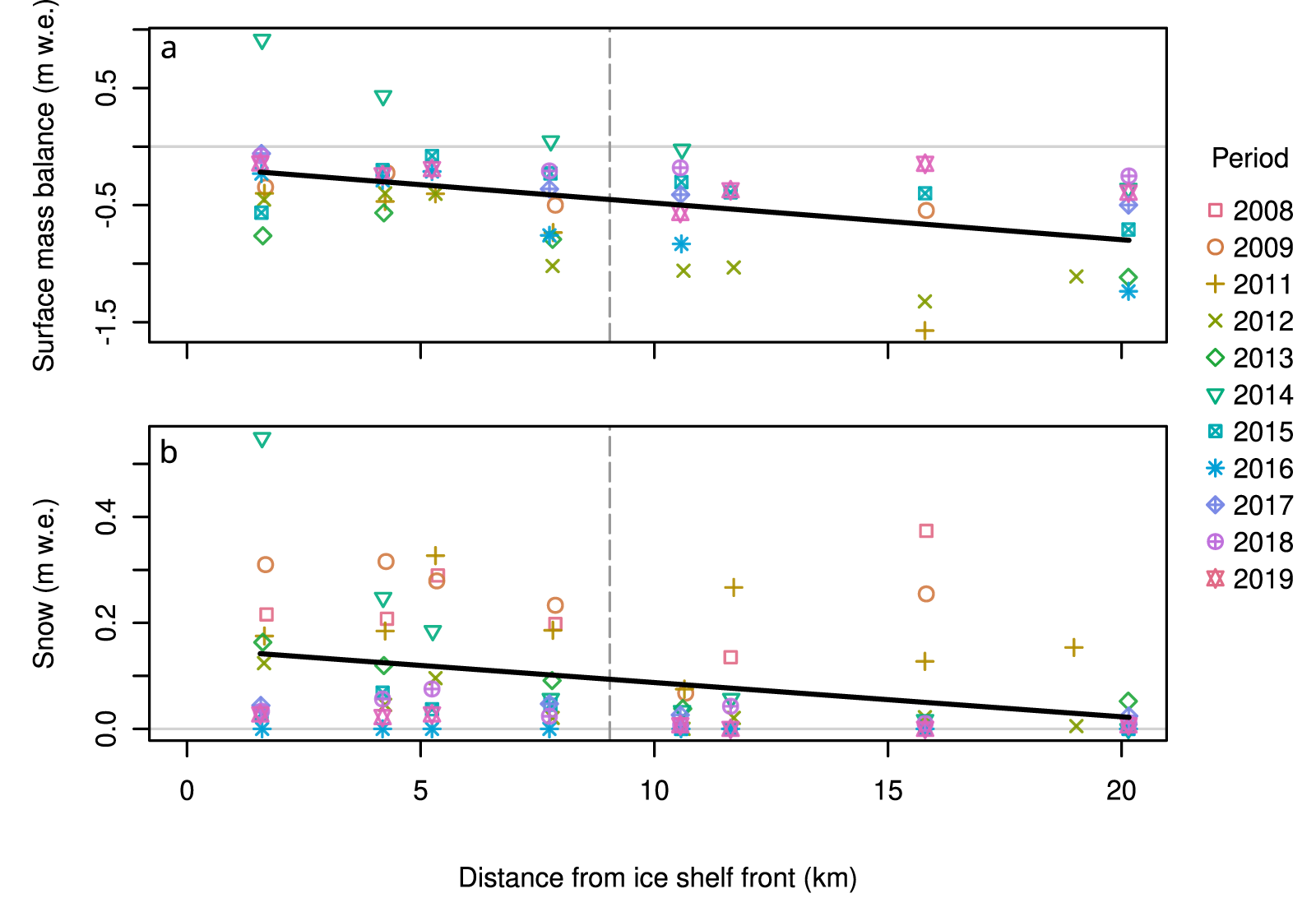
Surface mass balance was not uniform across the ice shelf, becoming progressively more negative with increasing distance inland from the northern, seaward edge (Fig. 5a). This same pattern was observed with snow depth (Fig. 5b). Separated by region, the Outer Unit had a total cumulative surface mass balance of −2.86 ± 1.78 m w.e. over the 11 year period, whereas the Central Unit had a total cumulative surface mass balance of −7.09 ± 1.00 m w.e. (Supplementary Table S1; Fig. 4a). In paired t-tests, the Outer Unit had a significantly more positive surface mass balance (t: 4.27, p: 0.001) and greater SWE (t: 2.77, p: 0.010) than the Central Unit.
(a) Annual surface mass balance and (b) annual snow water equivalent, with distance inland from the front (northern, seaward edge) of Milne Ice Shelf. Data from each field year are symbolized differently. A linear trend line for all years on record is plotted in black. The transition between the Outer and Central units of the ice shelf along the ice shelf gradient line (Figure 1a) is shown with a grey vertical dashed line.

Figure 5 Long description
Two scatter plots labeled a and b illustrate data related to the Milne Ice Shelf. The horizontal axis in both plots represents the distance from the ice shelf front in kilometers, ranging from 0 to 20. The vertical axis in plot a represents surface mass balance in meters water equivalent, ranging from negative 1.5 to 0.5. The vertical axis in plot b represents snow in meters water equivalent, ranging from 0 to 0.4. Each plot includes data points from different years, indicated by various symbols and colors. The legend on the right side identifies the years from 2008 to 2019 with corresponding symbols. A linear trend line is drawn in black across both plots, showing a decrease in values as the distance from the ice shelf front increases. A grey vertical dashed line marks a transition point at approximately 10 kilometers in both plots.
4.2. Microclimatology of the Milne Ice Shelf
A comparison of climate data recorded when M1-AWS, M3-AWS and M5-AWS were reporting simultaneously between 29 June 2012 and 2 August 2013 shows the gradients along the ice shelf. M1 and M3 had a 0.34–0.39°C lower mean air temperature compared to M5 over this 400 day timespan. M1 had the lowest mean relative humidity (87%), followed by M3 (88%) and M5 (90%). From 12 May to 2 August 2013 (83 days), all stations recorded incoming shortwave radiation, with M3 receiving 265 W m−2 on average, followed by M5 and M1, at 237 and 234 W m−2, respectively.
Differences between stations were also noted on a seasonal basis. During the summer, when temperatures often exceed 0°C, M1 was the warmest station, followed by M3, then M5. M5, located nearest the seaward edge of the ice shelf, recorded the coolest temperatures, likely due to the moderating influence of marine conditions and more frequent coastal fog and low cloud. This pattern is best illustrated by examining the temperature differences between the three ice shelf stations (Fig. 6a) and the PDD (Fig. 6b), which show clearly how much extra sensible heat is available in the Central Unit (M3 and M1) compared to the Outer Unit (M5).
Spatial and seasonal patterns in air temperature along Milne Fiord, 29 June 2012 to 2 August 2013. (a) Difference in air temperature between the index station at Purple Valley (PV-AWS) and M1-AWS (red), M3-AWS (green) and M5-AWS (blue). Locally weighted scatterplot smoothing (LOWESS) lines with a smoothing factor of 0.2 show seasonal changes in temperature patterns. (b) Positive degree-days (PDD) at each site (maximum values: PV 265. M1 85, M3 77 and M5 53·°C·d). Although M5 is warmer than M1 and M3 in general, it is much colder in the summer months, which has profound consequences for snow and ice melt.

Figure 6 Long description
Scatter plot with three overlaid smoothed lines and a legend listing M1 minus PV, M3 minus PV and M5 minus PV. The vertical axis label is delta temperature (degree Celsius) with tick labels negative 6, negative 4, negative 2, 0, 2, 4, 6. The horizontal axis shows time with tick labels Jul 2012, Jan 2013, Jul 2013. A horizontal reference line is drawn at 0. The plotted points appear across the full time range, with values spanning from about negative 6 to about 6 on the vertical axis. The three smoothed lines run across the plot, each staying mostly below 0 and varying between about negative 4 and about 0. Line graph with a legend listing PV, M1, M3 and M5. The vertical axis label is Positive degree days (degree Celsius dash d) with tick labels 0, 50, 150, 250. The horizontal axis shows time with tick labels Jul 2012, Jan 2013, Jul 2013. Four lines rise from near 0 at Jul 2012 to plateau levels, then drop to near 0 close to Jul 2013, then rise again by Jul 2013. The PV line rises to about 250, stays near that level, then drops to near 0, then rises to about 80. The M1 line rises to about 80, stays near that level, then drops to near 0, then rises to about 30. The M3 line rises to about 70, stays near that level, then drops to near 0, then rises to about 25. The M5 line rises to about 50, stays near that level, then drops to near 0, then rises to about 20.
4.3. Interannual climate
Based on air temperature observations at PV-AWS with complete years (January to December 2010–11 and 2013–18), the mean annual air temperature was −18.7°C. From 1 June 2009 to 31 August 2017, the mean summer (June–July–August) surface air temperature was 1.8°C. The warmest summer on record was in 2012, when mean air temperatures reached 3.4°C, while the coolest summer occurred in 2013, with a mean air temperature of −1.1°C (Fig. 2a).
Mean annual PDD at PV-AWS was 227.6°C·d, with large interannual variability (Fig. 2b). The years with highest PDD were in 2011, 2012 and 2016, with PDD >315°C·d and a maximum of 323.5°C·d in 2011 and 2012. The lowest PDD were recorded in 2013 at 105.5°C·d, followed by 118.4°C·d in 2014 (Fig. 2b). Mean monthly incoming shortwave radiation varied from 0 to 313 W m−2 (Fig. 2c), while the average monthly snow depth at PV was 3.6 cm, ranging from 0 cm during summers to 16 cm in May 2012 (Fig. 2d). No significant linear trends were found in the mean annual air temperature, summer air temperature or the PDD in this 10 year record.
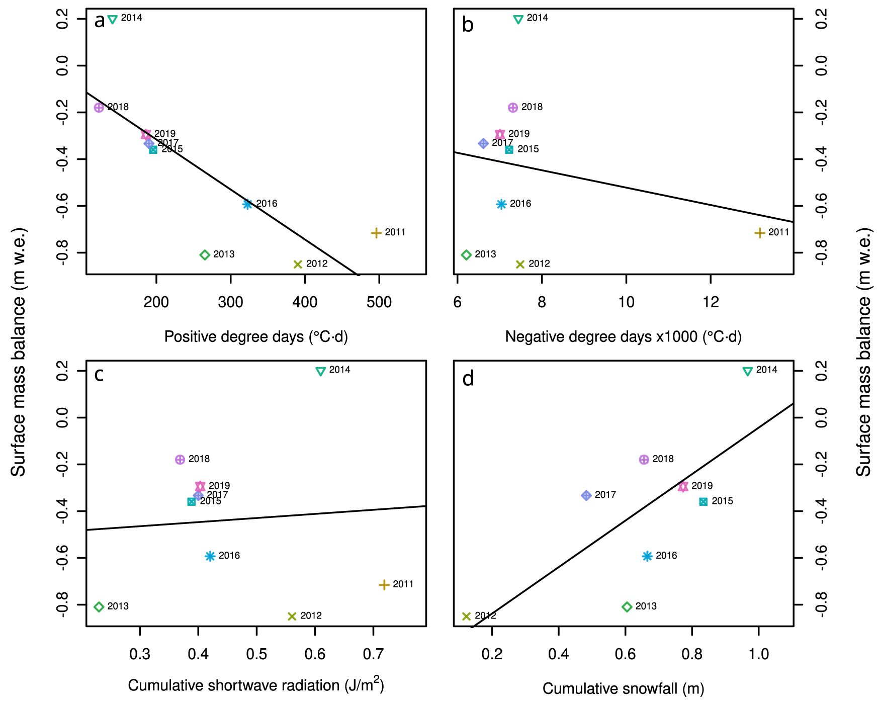
To seek an explanation for interannual differences between the surface mass balance years (Fig. 4), a series of linear regressions was calculated between this and cumulative climate variables from PV-AWS (Fig. 7). Unsurprisingly, the PDD during the interval between stake measurements is a good predictor of the surface mass balance (adjusted R 2: 0.56, p: 0.012). For every 1·3°C·d increase in PDD at PV, there was an average of 2 mm w.e. of melt on the ice shelf. The cumulative snowfall was also a significant predictor of surface mass balance (adjusted R 2: 0.46, p: 0.038). For every unit of cumulative snowfall at PV, there was a surface mass balance gain of an equal amount on the ice shelf. This high slope, coupled with a y-intercept of −1.0 m, likely reflects under-catch due to data outages (Supplementary Figure S1) and the relatively wind-blown location of PV-AWS. Nonetheless, interannual variability in snow accumulation at our index station PV-AWS is associated with surface mass balance on the Milne Ice Shelf, which is reasonable, given the underlying causal relationship between snowfall and surface mass balance.
Relationship between surface mass balance and cumulative climate variables. Each cumulative climate variable was measured at the index station at Purple Valley from May 2009 to July 2019. Individual data points are the sum of each variable over a surface mass balance interval vs the mean balance for all stake sites on the ice shelf. (a) Positive degree-days (PDD; °C·d). (b) Negative degree-days (NDD; °C·d). (c) Cumulative incoming shortwave radiation (CSR; J m−2). (d) Cumulative snowfall (m). Linear regression lines for positive degree-days and cumulative snowfall (a and d) are significant.

Figure 7 Long description
Scatter plot A with the horizontal axis labeled Positive degree days (degree C times d) and the vertical axis labeled Surface mass balance (m w.e.). The horizontal axis shows 200, 300, 400, 500. The vertical axis shows 0.2, 0.0, minus 0.2, minus 0.4, minus 0.6, minus 0.8. Points are labeled by year and a straight fitted line runs downward from left to right. The plotted years include 2014 near left parenthesis about 150, 0.2 right parenthesis; 2018 near left parenthesis about 120, minus 0.2 right parenthesis; 2019 near left parenthesis about 180, minus 0.3 right parenthesis; 2017 near left parenthesis about 190, minus 0.35 right parenthesis; 2015 near left parenthesis about 200, minus 0.38 right parenthesis; 2016 near left parenthesis about 320, minus 0.6 right parenthesis; 2013 near left parenthesis about 260, minus 0.85 right parenthesis; 2012 near left parenthesis about 390, minus 0.85 right parenthesis; 2011 near left parenthesis about 500, minus 0.72 right parenthesis. The fitted line direction matches a decrease in surface mass balance values as positive degree days increase. Scatter plot B with the horizontal axis labeled Negative degree days times 1000 (degree C times d) and the vertical axis labeled Surface mass balance (m w.e.). The horizontal axis shows 6, 8, 10, 12. The vertical axis shows 0.2, 0.0, minus 0.2, minus 0.4, minus 0.6, minus 0.8. Points are labeled by year and a straight fitted line runs downward from left to right. The plotted years include 2014 near left parenthesis about 7, 0.2 right parenthesis; 2018 near left parenthesis about 7, minus 0.2 right parenthesis; 2019 near left parenthesis about 7.2, minus 0.3 right parenthesis; 2017 near left parenthesis about 7.0, minus 0.35 right parenthesis; 2015 near left parenthesis about 7.2, minus 0.38 right parenthesis; 2016 near left parenthesis about 7.0, minus 0.6 right parenthesis; 2013 near left parenthesis about 6.5, minus 0.82 right parenthesis; 2012 near left parenthesis about 7.5, minus 0.85 right parenthesis; 2011 near left parenthesis about 13, minus 0.72 right parenthesis. Most points cluster around negative degree days values near 6.5 to 7.5 with surface mass balance between about minus 0.2 and minus 0.85 and one point at about 13 with surface mass balance about minus 0.72. Scatter plot C with the horizontal axis labeled Cumulative shortwave radiation (J over m superscript 2) and the vertical axis labeled Surface mass balance (m w.e.). The horizontal axis shows 0.3, 0.4, 0.5, 0.6, 0.7. The vertical axis shows 0.2, 0.0, minus 0.2, minus 0.4, minus 0.6, minus 0.8. Points are labeled by year and a straight fitted line runs slightly upward from left to right. The plotted years include 2014 near left parenthesis about 0.62, 0.2 right parenthesis; 2018 near left parenthesis about 0.38, minus 0.2 right parenthesis; 2019 near left parenthesis about 0.40, minus 0.3 right parenthesis; 2017 near left parenthesis about 0.42, minus 0.35 right parenthesis; 2015 near left parenthesis about 0.41, minus 0.38 right parenthesis; 2016 near left parenthesis about 0.45, minus 0.6 right parenthesis; 2013 near left parenthesis about 0.28, minus 0.82 right parenthesis; 2012 near left parenthesis about 0.58, minus 0.85 right parenthesis; 2011 near left parenthesis about 0.72, minus 0.72 right parenthesis. The fitted line is close to flat compared with the other plots. Scatter plot D with the horizontal axis labeled Cumulative snowfall (m) and the vertical axis labeled Surface mass balance (m w.e.). The horizontal axis shows 0.2, 0.4, 0.6, 0.8, 1.0. The vertical axis shows 0.2, 0.0, minus 0.2, minus 0.4, minus 0.6, minus 0.8. Points are labeled by year and a straight fitted line runs upward from left to right. The plotted years include 2014 near left parenthesis about 1.0, 0.2 right parenthesis; 2018 near left parenthesis about 0.7, minus 0.2 right parenthesis; 2019 near left parenthesis about 0.8, minus 0.3 right parenthesis; 2017 near left parenthesis about 0.45, minus 0.35 right parenthesis; 2015 near left parenthesis about 0.85, minus 0.38 right parenthesis; 2016 near left parenthesis about 0.7, minus 0.6 right parenthesis; 2013 near left parenthesis about 0.6, minus 0.82 right parenthesis; 2012 near left parenthesis about 0.2, minus 0.85 right parenthesis. The fitted line direction matches an increase in surface mass balance values as cumulative snowfall increases. Across the four scatter plots, the fitted line slopes are steepest in the positive degree days plot and the cumulative snowfall plot and closest to flat in the cumulative shortwave radiation plot.
4.4. Ground penetrating and SAR
The GPR profiles collected in May 2013 show clear layering from ∼2 to ∼20 m below the surface in the Outer Unit of the Milne Ice Shelf, particularly nearest the ocean (Fig. 3). This layering rises towards the surface near the centre of the ice shelf (Fig. 3b) and is consistent with the characteristic pattern observed between the boundary of annual firn layers on Arctic glaciers (e.g. Devon Ice Cap, Sylvestre and others, Reference Sylvestre, Copland, Demuth and Sharp2013; Austfonna, Dunse and others, Reference Dunse, Schuler, Hagen, Eiken, Brandt and Høgda2009). In contrast, the GPR profiles recorded low backscatter across the Central Unit near the inland edge of the ice shelf (apart from a few point returns assumed to be from small crevasses), with only one strong near-surface layer at the snow–ice interface from the last summer surface (Fig. 3d). The lack of internal scatter below the surface indicates that no strong dielectric contrasts were present in this part of the ice shelf, implying little variability in its internal properties. The 7 m-long core extracted from the M1 site in May 2013 was consistent with this, as it was composed of clear ice throughout with no internal layering (Supplementary Figure S2).
The areas of subsurface layering detected in the 2013 GPR results correspond closely with the location of high SAR backscatter across the Outer Unit of the Milne Ice Shelf in SAR satellite imagery (Fig. 3a). Based on the RADARSAT-2 image of the ice shelf from March 2013, a transect of backscatter values shows that the first 6 km of the Outer Unit (from the northern, seaward edge) had the highest values, with an average of −6.17 dB (Fig. 3a inset). In contrast, the remainder of the transect had relatively low backscatter, with average values of −11.06 dB across the Central Unit. Additional SAR scenes from 1992, 1998, 2006, 2015 and 2018 show that the transition between high and low backscatter has remained in essentially the same position over the 26 year period (Fig. 8).
Backscatter values extracted from a 13 km long transect extending from the Outer Unit to the Central Unit: (a) ERS-1: 29 January 1992; (b) Radarsat-1: 16 April 1998; (c) Radarsat-1: 14 January 2006; (d) Radarsat-2: 22 March 2015; (e and f) Radarsat-2: 27 November 2018. Ice shelf outlines from 1992 to 2015 from Mueller et al. (Reference Mueller, Copland and Jeffries2017b). Each graph shows the backscatter values (σ0) with a 35 m running average, extracted from each transect for each year (a–e) and the average of these values from 1992 to 2018 (f). The distance on the horizontal axis represents the distance from the rear of the ice shelf.

Figure 8 Long description
Six panels show satellite images and corresponding graphs of backscatter values along a transect on an ice shelf from 1992 to 2018. Each panel includes a satellite image with a colored outline and a graph below it. The images are labeled with years: 1992, 1998, 2006, 2015, 2018 and a combined average from 1992 to 2018. The backscatter values are represented in decibel, ranging from -20 to 5, with color-coded legends indicating different value ranges. The graphs plot backscatter values (sigma in decibel) against distance (kilometers), showing variations over the transect. The x-axis is labeled ′Distance (km)′ ranging from 7 to 20 kilometers and the y-axis is labeled ′sigma (dB)′ ranging from -18 to 2 decibel. Each graph shows a trend line with scattered data points, indicating changes in backscatter values over time. The outlines on the images represent ice shelf extents for each year, with the final panel showing the mean backscatter values from 1992 to 2018.
5. Discussion
5.1. Surface mass balance gradients along the Milne Ice Shelf
From our results, it is evident that a pronounced gradient in SWE, surface mass balance, climatic variables and physical characteristics exists along the ocean-to-inland length of the Milne Ice Shelf. The mean annual surface mass balance ranged from a mean of −0.26 m w.e. (range: −0.71 to +0.46 m w.e.) in the Outer Unit, nearest the ocean, to a mean of −0.64 m w.e. (range: −1.13 to −0.19 m w.e.) in the Central Unit, furthest inland. GPR transects, SAR backscatter and ice core records show that the Outer Unit is primarily composed of meteoric ice with internal layering reflecting long-term net accumulation, while the Central Unit is composed of solid ice with no internal layering, indicative of net annual ablation. The internal layering present in the Outer Unit rises towards the surface with distance inland along the GPR transect (Fig. 3), indicative of the long-term decrease in accumulation with distance from the northern, seaward edge. This surface mass balance gradient is reflected not only in the recent thickness of the ice shelf but also in how that thickness has changed over time. GPR transects collected across the ice shelf in 2008/09 reported average ice thicknesses of 70–80 m in the Outer Unit, compared to ∼50 m in the Central Unit (Mortimer and others, Reference Mortimer, Copland and Mueller2012). Between 1983 and 2008/09, Mortimer and others (Reference Mortimer, Copland and Mueller2012; their fig. 4c) also showed that thickness over most of the Outer Unit changed between −7.5 and +7.5 m, whereas much of the Central Unit thinned by 15–30 m.
To better understand these gradients, we applied a linear mixed effects model to predict the quasi-annual surface mass balance data from the distance of each stake from the northern, seaward edge of the ice shelf (Fig. 9). The optimized, parsimonious model explains 23% of the variance in surface mass balance for 51 observations at 8 sites from distance alone. A total of 64% of the variance was accounted for by nine different years, leaving 13% of the variance unexplained. The model had a mean absolute error of 0.111 m w.e. and a root-mean-square error of 0.144 m w.e. Upon cross-validation, these metrics rose to 0.179 and 0.241 m w.e., respectively. This shift in model skill is indicative of some model overfitting, although the R 2 values did not change appreciably, which suggests that the model is reasonably robust (Kabacoff, Reference Kabacoff2015).
Output of the linear mixed effects model that predicts the annual surface mass balance with distance from the ice shelf front (northern, seaward edge). The overall slope of this spatial gradient (the model’s fixed effect) is 37 mm w.e. km−1 along the ice shelf (dashed black line). The model considers interannual variation in environmental conditions between stake measurements. Here, for example, the value of positive degree-days between stake measurements was used as a random effect and a line was fit to each year. The transition between the Outer and Central units of the ice shelf along the ice shelf gradient line (Figure 1a) is shown with a grey vertical dashed line.

Figure 9 Long description
The graph displays surface mass balance in meters water equivalent (m w.e.) on the vertical axis, ranging from negative 1.5 to positive 1.0, against distance from the ice shelf front in kilometers on the horizontal axis, ranging from 0 to 20. Multiple lines represent different periods from 2011 to 2019, each marked with distinct symbols. The legend indicates the period with corresponding symbols: 2011 (plus), 2012 (times), 2013 (diamond), 2014 (triangle), 2015 (square), 2016 (asterisk), 2017 (cross), 2018 (circle) and 2019 (star). A dashed black line represents the overall slope of the spatial gradient. Each line shows a trend of decreasing surface mass balance with increasing distance from the ice shelf front. The transition between the Outer and Central units of the ice shelf is marked by a grey vertical dashed line at approximately 10 kilometers.
The model had a fixed-effect slope of −0.037 m w.e. km−1 (95% confidence interval: −0.057 to −0.019) and an intercept of −0.114 m w.e. (95% confidence interval: −0.364 to +0.137) (Fig. 9). The model explains 87% of the variance in surface mass balance at the eight sites across the ice shelf. Since the confidence interval of the intercept includes 0, we can conclude that the modelled ice surface at the very outer, seaward edge of the ice shelf is approximately in balance. The spatial gradient, revealed by the slope, indicates that surface ablation increases by an average of 37 mm w.e. for every km between the seaward and landward edge of the ice shelf. Although slopes were consistently negative, their magnitude varied considerably, ranging from −0.014 in 2018 to −0.074 m w.e. km−1 in 2011 (2.7× less to 1.9× more than the overall slope).
The model was fit using the nine random effects groups (years) of surface mass balance data. These groups were then represented by the PV-AWS index PDD values from each of the surface mass balance years (Figs 9 and 10a). Not only is PDD associated with greater ice surface loss (Fig. 7a), but it is also significantly related (adjusted R 2: 0.55, p: 0.013) to the spatial gradient in surface mass balance (Fig. 10a). The years in the lower right portion of the plot (i.e. 2011, 2012 and 2016) are those with a large PDD and a very large spatial gradient (Fig. 10a). The years to the upper left (i.e. 2015, 2017, 2018 and 2019) have a low PDD and a low surface mass balance gradient. In general, the higher the PDD, the bigger the spatial gradient in surface mass balance becomes.
Relationship between the cumulative climate variables and the spatial gradient in surface mass balance along the ice shelf. (a) Positive degree-days (PDD; °C·d). (b) Negative degree-days (NDD; °C·d). (c) Cumulative incoming shortwave radiation (CSR; J m−2). (d) Cumulative snowfall (CSF; m). Linear regression lines for PDD and CSR (a and c) are significant, suggesting that these variables are associated with the interannual variability in the strength of the surface mass balance gradient. As these variables increase, the spatial gradient intensifies. Vertical and horizontal dashed grey lines indicate the mean model slope (0.037 m w.e. km−1 for PDD, NDD and cumulative shortwave radiation; 0.032 for cumulative snowfall) and the mean of the cumulative climate variables, respectively. The position of individual years provides insight into what variables were important to establishing the spatial gradient in any given year. For example, in most years, the PDD is strongly associated with the spatial gradient, but in 2014, the snowfall might have contributed more to the above-average gradient, despite this variable not being associated with the gradient overall.

Figure 10 Long description
The scatterplot matrix consists of four panels, each illustrating the relationship between cumulative climate variables and the spatial gradient in surface mass balance along the ice shelf. Panel a: Positive degree days (PDD) in degrees Celsius times days are plotted on the x-axis, ranging from 0 to 500. The y-axis shows the surface mass balance gradient in m w.e./km, ranging from -0.07 to 0.03. Year-coded points are plotted, with a negative trend line indicating a decrease in gradient with increasing PDD. Notable points include 2011 at high PDD with the most negative gradient. Panel b: Negative degree days (NDD) times 1000 in degrees Celsius times days are on the x-axis, ranging from 6 to 14. The y-axis is the same as panel a. The trend line is negative, showing a decrease in gradient with increasing NDD. Year 2011 is again notable for its extreme values. Panel c: Cumulative incoming shortwave radiation (CSR) in joules per m superscript 2 is on the x-axis, ranging from 0.3 to 0.7. The y-axis remains consistent. The negative trend line suggests a decrease in gradient with increasing CSR. Year 2011 stands out with high CSR and negative gradient. Panel d: Cumulative snowfall in m is on the x-axis, ranging from 0.2 to 1.0. The y-axis is unchanged. The trend line is slightly positive, indicating a slight increase in gradient with more snowfall. Year 2014 is notable for its position. Each panel includes vertical and horizontal dashed grey lines indicating the mean model slope and mean of the cumulative climate variables. The regression lines for PDD and CSR are significant, suggesting these variables are associated with inter-annual variability in the surface mass balance gradient.
To investigate if other climate variables also influence the mass balance gradient, the model was re-fit using NDD, CSR and cumulative snowfall to account for the random effect. NDD and CSR were available for the same 9 years as PDD, so this substitution did not change the overall model slope or the variance that the model explains. The relationship between NDD and the spatial mass balance gradient (Fig. 10b) is biased by the 2011 value (the only period in the record spanning 2 years), but even without this data point the relationship is not meaningful. CSR has a significant relationship to the surface mass balance gradient (adjusted R 2: 0.54, p: 0.014; Fig. 10c), while cumulative snowfall did not (Fig. 10d). This shows that the spatial gradient in surface mass balance is related to PDD and CSR, but not NDD or cumulative snowfall.
5.2. Glacier facies along the Milne Ice Shelf
The surface mass balance gradient along the Milne Ice Shelf, together with marked differences in its physical characteristics and ice thickness, suggests that, similar to traditional glaciers (and other Ellesmere ice shelves; Mueller and Vincent, Reference Mueller and Vincent2006), it can be divided into an accumulation zone (Outer Unit, seaward margin) and ablation zone (Central Unit, inland margin), divided by a transition area or equilibrium line. This is despite the fact that the ice shelf is almost completely flat and reaches a height of no more than ∼10 m a.s.l. These distinctions are particularly apparent in 2014, when the surface of the Central Unit lost mass while the Outer Unit gained mass (Fig. 4b). In this year, the equilibrium line was positioned between M3 (−0.03 m w.e.) and M8 (+0.05 m w.e.). This compares well with the GPR and SAR data that show sub-surface layers tapering off and a distinct drop in the 1991–2018 mean backscatter values ∼12–13 km away from the southern edge of the ice shelf, respectively (Figs 3 and 8f).
The mean gradient in annual surface mass balance across the ice shelf, derived from the linear mixed effects model (Fig. 9), is 37 mm w.e. of additional melt per year per km from the front of the ice shelf to the rear. This may not seem like a large effect, but given that the ice shelf was ∼20 km long prior to August 2020, this amounts to ∼0.74 m w.e. a−1 more loss at the southern, inland edge of the ice shelf than at the northern, seaward edge, which sums to 8.14 m w.e. of enhanced ablation at the far southern end of the ice shelf over the study period. The slope of this gradient varies from year to year and was positively related to the PDD and CSR values measured at the PV-AWS index station. When PDD and CSR increased, the slope of the gradient became more pronounced. The enhanced melt observed towards the landward end of the ice shelf may reflect the influence of warmer air originating from the neighbouring ice-free terrain in PV. Air temperatures and PDD totals at PV-AWS were consistently higher than those measured at the ice shelf stations (Fig. 6), suggesting that the inland portion of the ice shelf is subjected to a greater supply of sensible heat during the melt season.
This effect places the southern, inland portion of the ice shelf in the Central Unit in double jeopardy in a warming climate: if the PDD at nearby PV increases, the surface mass balance will decrease on average across the ice shelf at a rate of 2 mm w.e. °C−1 d−1 (Fig. 10a), but the loss will be even more pronounced at the landward side of the ice shelf due to the enhanced spatial gradient that will be incurred. If the CSR increases, the model predicts that the spatial gradient will also be enhanced, although we found no significant relationship between mass loss and CSR on an annual basis.
The lower ablation rate across the seaward Outer Unit is characteristic of the ‘Arctic Ocean Effect’, whereby the ocean acts as a local moisture source that leads to increased precipitation along a narrow zone along the coastline (Koerner, Reference Koerner1979). This moisture source also results in more frequent fog and low stratus clouds along the coastline, as often observed during our fieldwork, which explains the lower shortwave radiation inputs at the Outer Unit than the Central Unit. The biggest absolute difference in shortwave radiation input on record occurred in May 2013, when mean shortwave radiation values were 43 W m2 (16%) lower at M5-AWS compared to M3-AWS. This is also the month when the largest difference in relative humidity occurred between these stations, with frequent near-coastal fog observed during fieldwork at this time of year.
The high incidence of coastal fog and low cloud has also been observed elsewhere near Sverdrup Glacier (northwest Devon Ice Cap), Ward Hunt Island and Meighen Ice Cap, where it has been suggested to be a factor in reducing ablation rates (Sagar, Reference Sagar1962; Paterson, Reference Paterson1969; Hattersley-Smith and Serson, Reference Hattersley-Smith and Serson1970; Koerner, Reference Koerner2005; Mueller and Vincent, Reference Mueller and Vincent2006; Braun, Reference Braun, Copland and Mueller2017). Koerner (Reference Koerner2005) found that the mass balance gradient (from 1961 to 2003) was disrupted by limited ablation below 350 m at Sverdrup Glacier and could possibly be linked to fog being generated from increasing open water (in summer) in Jones Sound. According to the spatial distribution of surface mass balance at Ward Hunt Ice Shelf, ablation stakes installed in marine ice sites that surround Ward Hunt Island had a significantly higher ablation (mean: 0.75 ± 0.17 m), compared to the stake clusters installed on meteoric ice sites nearer the ocean (0.29 ± 0.05 m), which Mueller and Vincent (Reference Mueller and Vincent2006) suggested could be linked to the distribution of fog. According to Alt (Reference Alt1979), Meighen Ice Cap, lying at 268 m a.s.l., owes its existence and positive mass balance years to synoptic conditions that produce fog.
PDD show large interannual variability, and the month of July accounts for the majority of summer warmth. There is a strong and significant relationship between PDD at PV-AWS and mean annual surface mass balance on the ice shelf (Fig. 7a). Assuming the 2009–11 surface mass balance was equal (−0.358 m w.e.) before and after 24 May 2010, each mass balance period is approximately 1 year. The one positive balance year in 2014 was associated with the second lowest PDD on record (141°C·d), while the years near the median PDD value (202°C·d) had a surface mass balance of ∼−0.36 m w.e. (2011 and 2015). The years above the median PDD (2010, 2012, 2013 and 2016) had a surface mass balance ranging from −0.358 m w.e. in 2010 to a maximum of −0.850 m w.e. in 2012, corresponding to a PDD of 390°C·d (Fig. 7a).
The relationship between PDD and corresponding mass balance is similar to that observed on the St Patrick Bay Ice Caps, north-east Ellesmere Island, where positive mass balance years were associated with summer PDD <190°C·d (Bradley and Serreze, Reference Bradley and Serreze1987). In examining the connection between PDD and ice shelf calving along the coastline of northern Ellesmere Island, Copland and others (Reference Copland, Mueller and Weir2007) found that periods of frequent ice shelf calving occurred between 1948 and 1963 when PDD were typically >200°C·d, followed by a period of little calving when PDD rarely exceeded 200°C·d. The period of increased ice shelf break-up between the mid-1990s and mid-2000s occurred after PDD returned to >200°C·d, with the complete loss of the Ayles Ice Shelf in 2005 when PDD exceeded 300°C·d (Copland and others, Reference Copland, Mueller and Weir2007). Our PV-AWS regularly exceeded 200°C·d half of the time, and exceeded 300°C·d twice, over the study period.
5.3. Historical changes
The consistency between areas of high and low backscatter in the GPR data and SAR imagery agrees with the study by Mueller and Vincent (Reference Mueller and Vincent2006), who used SAR imagery to map out glacier facies across the Milne Ice Shelf. Similar to studies on Arctic glaciers (Engeset and others, Reference Engeset, Kohler, Melvold and Lunden2002; Casey and Kelly, Reference Casey and Kelly2010), high backscatter in SAR imagery is indicative of the presence of firn in the accumulation area, whereas low backscatter indicates the presence of glacier ice in the ablation area. With the availability of SAR data across a 26 year period, this enables a determination of whether the locations of the accumulation and ablation zones, and equilibrium line, have changed over time (Fig. 8). This analysis indicates that the equilibrium line, defined as the boundary between the Outer and Central units, has remained in broadly the same position since at least 1992. However, the area of the Central Unit has shrunk as a result of fracture development and propagation and break-up from the rear of the ice shelf (Fig. 11).
Temporal changes in the Central Unit of the Milne Ice Shelf, highlighting the development and widening of rifts and the decrease in the extent of the ice shelf: (a) ASTER L1T, 10 July 2009; (b) ASTER L1T, 15 July 2012; and (c) Landsat-8, 31 July 2018 (panchromatic band).

Figure 11 Long description
Three satellite maps illustrate changes in the Milne Ice Shelf, located in Arctic Canada. Image A from 2009 shows the Central Unit and Epishelf Lake, with tributary glaciers feeding into the ice shelf. Blue outlines mark glacier tongues and rift locations. Image B from 2012 depicts expanding ice-dammed lakes, rift widening and glacier disconnection. Blue lines indicate rift expansion, while dashed lines show disintegration areas. Image C from 2018 highlights further rift expansion and reduced ice shelf extent, marked by red outlines. The ice shelf boundary retreats and tributary glaciers are disconnected. North is oriented at the top and scale bars are present in each image. The maps demonstrate significant structural changes over time, with rifts lengthening across the shelf and the ice shelf boundary retreating.
Mortimer and others (Reference Mortimer, Copland and Mueller2012) measured area changes across the Milne Ice Shelf between 1950 and 2009 and found that most losses occurred at its rear, where the former Inner Unit and part of the Central Unit deteriorated and were replaced by an epishelf lake, resulting in a loss of 59 km2. Since 2009, the break-up at the rear of the ice shelf has continued; between 2009 and 2018, the area of the Central Unit decreased by 9.8 km2, similar to the long-term loss rate of ∼1 km2 a−1. Additional losses resulted from the expansion of marginal epishelf lakes within the Central Unit and along the boundary of the Central and Outer units. The development and expansion of fractures penetrating the Central Unit accounted for an additional ∼2 km2 of area loss. This landward break-up is consistent with the persistent spatial gradient in surface mass balance identified in this study and with the deterioration patterns observed at other ice shelves on northern Ellesmere Island, suggesting that similar climatic controls (e.g. warm air advection from ice-free areas) may be driving preferential inland ice shelf loss across the region.
At the back of Petersen Ice Shelf, ∼15 km southwest of the Milne Ice Shelf, thin meltwater-filled troughs fractured apart individual ridges that detached and drifted as ice islands (White and others, Reference White, Copland, Mueller and Van Wychen2015; Mueller and others, Reference Mueller, Copland, Jeffries, Copland and Mueller2017a). The Ward Hunt Ice Shelf, ∼80 km to the east, also developed extensive fractures at its rear, between Disraeli Fiord and Ward Hunt Island (centrally located within the Ward Hunt Ice Shelf; Mueller and others, Reference Mueller, Vincent and Jeffries2003). By July and August 2008, 25% of the fiord ice cover had been lost (Vincent and others, Reference Vincent, Whyte, Lovejoy, Greer, Laurion, Suttle, Corbeil and Mueller2009), followed by ice shelf break-up along both the northern and southern edges into Disraeli Fiord (Mueller and others, Reference Mueller, Vincent and Jeffries2003).
Historically, the front of the Milne Ice Shelf remained quasi-stable from 1974 to 2015 (Jeffries, Reference Jeffries1986b; Mortimer and others, Reference Mortimer, Copland and Mueller2012), with the exception of a 3 km2 calving near Cape Evans in 2012–13 (Mueller and others, Reference Mueller, Copland, Jeffries, Copland and Mueller2017a). However, this long period of relative frontal stability ended abruptly in late July 2020, when a calving event removed nearly half of the ice shelf, consisting predominantly of the seaward Outer Unit (Hamilton and others, Reference Hamilton, Mueller and Laval2021). The break occurred along pre-existing fractures in the Outer and Central units, with the collapse likely driven by a combination of long-term thinning, particularly at the rear of the ice shelf, and the persistence and widening of rifts (Figs 1a and 11). This left the ice shelf unable to maintain structural integrity during a period of open water at its front, when the usual buttressing from sea ice was absent, a phenomenon also observed during calving events of other ice shelves and ice tongues on northern Ellesmere Island (Copland and others, Reference Copland, Mueller and Weir2007, Reference Copland, Mortimer, White, Richer-McCallum, Mueller, Copland and Mueller2017; White and others, Reference White, Copland, Mueller and Van Wychen2015; White and Copland, Reference White and Copland2019; Hamilton and others, Reference Hamilton, Mueller and Laval2021). Since the 2020 calving event, the remaining Milne Ice Shelf has remained broadly similar in extent and configuration to that shown in Fig. 1c.
It is clear that the spatial gradient in surface mass balance has been a long-term phenomenon in Milne Fiord, where it was likely responsible for ablating the Inner Unit of the Milne Ice Shelf between the Central Unit and the Milne Glacier ice tongue. This expanse of ice was identified as ice shelf by Jeffries (Reference Jeffries1986a) based on air photos from 1959 and surface roll morphology, in spite of in situ and airborne radar evidence that most of this ice was <10 m thick. It is possible that the Inner Unit was, at one time, much thicker, such that a thick ice shelf filled the entirety of Milne Fiord from the Milne Glacier in the south to the fiord mouth in the north. In this scenario, the surface mass balance gradient we describe could have preferentially degraded this ice, transitioning a thick Inner Unit from ice shelf to epishelf lake ice over the last 60+ years. We detected no statistically significant warming in our short PV record, but climate reanalyses in the study area show warming over longer multi-decadal periods (White and Copland, Reference White and Copland2019), and given the ongoing rate of warming in the Arctic and the link between PDD and the spatial mass balance gradient, it seems likely that this effect has intensified over the past decades. The preferential melt, thinning and loss of cryospheric features that are positioned well within fiords and embayments nearby suggest that the spatial gradient in mass balance is a significant effect along the northern coast of Ellesmere Island.
Despite the changes described above, the Milne Ice Shelf is the last of the northern Ellesmere Island ice shelves to have remained largely intact prior to its 2020 break-up. This is likely because it contained the thickest ice of any of these ice masses, with ice depths reaching >80 m across parts of the Outer Unit in 2008/09 (Mortimer and others, Reference Mortimer, Copland and Mueller2012). This compares to 42–45 m for an ice island recently calved from the Ayles Ice Shelf (Copland and others, Reference Copland, Mueller and Weir2007) and a mean of 29 m for the Petersen Ice Shelf in 2011 (White and others, Reference White, Copland, Mueller and Van Wychen2015). This substantial thickness reflects the fact that five main tributary glaciers fed ice into the Milne Ice Shelf as recently as the 1950s (Mortimer and others, Reference Mortimer, Copland and Mueller2012; Copland and others, Reference Copland, Mortimer, White, Richer-McCallum, Mueller, Copland and Mueller2017). Other studies have also highlighted how Milne Fiord has a protective physiography, by providing points of stability along its margins where the ice shelf connects with the walls of the fiord (Jeffries, Reference Jeffries1986a; Veillette and others, Reference Veillette, Mueller, Antoniades and Vincent2008). The north-south fiord orientation has also protected the ice shelf from the predominantly westward movement of pack ice along northern Ellesmere Island (Jeffries, Reference Jeffries1986a; Veillette and others, Reference Veillette, Mueller, Antoniades and Vincent2008; Mortimer and others, Reference Mortimer, Copland and Mueller2012).
6. Conclusions
Our findings indicate that the mass balance of the Milne Ice Shelf is predominantly controlled by the microclimatology along a horizontal gradient from the ice shelf’s seaward front to its inland rear. The persistence and relative stability of the seaward Outer Unit until 2020 is linked to cooler temperatures, lower shortwave radiation and higher snowfall, which suppress ablation, keeping the surface at the front of the ice shelf close to long-term balance. In contrast, the inland Central Unit is subject to warmer temperatures, higher shortwave radiation and lower snowfall. Past studies have shown that input from tributary glaciers contributed to portions of the Central Unit (Jeffries, Reference Jeffries1986b; Mortimer and others, Reference Mortimer, Copland and Mueller2012; Richer-McCallum, Reference Richer-McCallum2015), but since 2011, all but one of these tributary glaciers have become disconnected and are no longer a significant source of replenishment (Mortimer and others, Reference Mortimer, Copland and Mueller2012; Fig. 11). The lack of glacier inflow, in combination with relatively warmer temperatures and higher shortwave radiation, has led to higher rates of ablation there compared to the Outer Unit.
The Milne Ice Shelf is a remnant of what was once the continuous Ellesmere Ice Shelf that fringed the northern coast of Ellesmere Island at the start of the 20th century and developed under colder conditions of the past (Vincent and others, Reference Vincent, Gibson and Jeffries2001; Mueller and others, Reference Mueller, Copland, Jeffries, Copland and Mueller2017a). Although the Milne Ice Shelf has undergone changes over the past century, it has, until recently, been more stable than any of the other ice shelves on northern Ellesmere Island. This relative stability has changed substantially, however, as marginal epishelf lakes expanded and the rear of the ice shelf began to disintegrate rapidly starting in 2012. In 2020, a large calving event drastically changed the character of the ice shelf, with the loss of most of the Outer Unit. If the recent rate of ice loss in the remainder of the Outer Unit (∼0.26 ± 0.18 m w.e. a−1) is assumed to remain constant, the ∼63 m thick Outer Unit (Mortimer and others, Reference Mortimer, Copland and Mueller2012) would take 242 years to disappear from surface ablation alone. In contrast, the inland Central Unit would disappear in only 70 years from surface ablation alone given its recent average mass balance of 0.64 ± 0.10 m w.e. a−1 and mean thickness of ∼45 m (Mortimer and others, Reference Mortimer, Copland and Mueller2012). Based on the relationship between PDD and surface mass balance (Fig. 7a), additional PDD in the future will increase melt by approximately 2 mm w.e. °C−1 d−1 and enhance the spatial gradient in mass balance, further accelerating the thinning underway at the inland end of the ice shelf. However, the Milne Ice Shelf, which has lost a significant portion of its surface area and is already heavily fractured (Fig. 1), is likely to collapse well before this time. The ice shelf continues to be vulnerable to calving at both its landward and seaward edges.
Supplementary material
The supplementary material for this article can be found at https://doi.org/10.1017/jog.2026.10195.
Acknowledgements
We thank Colleen Mortimer, Sierra Pope, Andrew Hamilton, Miriam Richer-McCallum, Tyler De Jong, Dorota Medrzycka, Peter Wray, Jinsuk Kim, Drew Friedrichs, Yulia Antropova, Jérémie Bonneau, Abigail Dalton and members of the Canadian Rangers for assistance in data collection, and the Polar Continental Shelf Program (PCSP) for assistance with field logistics. We also thank Martin Jeffries, Sergey Samsonov, Alaska Satellite Facility and the Canadian Space Agency for providing ERS-1 and RADARSAT-1/2 data. This work was funded by grants from the Natural Sciences and Engineering Research Council (NSERC) of Canada, Canada Foundation for Innovation, Ontario Research Fund, University of Ottawa, Polar Continental Shelf Program, the Royal Canadian Geographical Society and ArcticNet, a Network of Centres of Excellence of Canada. Adrienne White was supported by graduate scholarships from NSERC, the Ontario Graduate Scholarship, the Association of Canadian Universities for Northern Studies, the Garfield Weston Foundation, and awards from the Northern Scientific Training Program.




 Open access

