II. EXPERIMENTAL DETAILS AND MEASUREMENTS

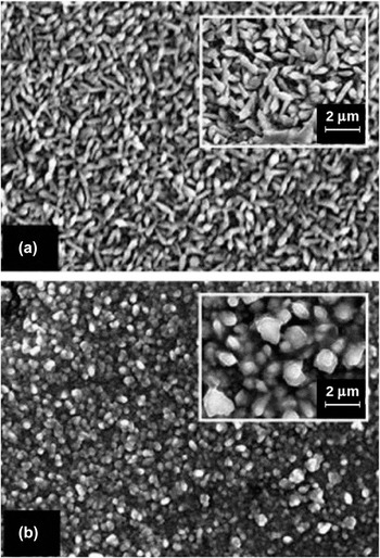
Electrodeposits of Co₈₇Cu₁₃ alloys were obtained on polished copper foil substrates from solutions containing 0.5 M CoSO₄·7H₂O, 0.05 M CuSO₄·6H₂O, and 1.0 M Na₂SO₄ using a chrono-amperometric method with cathodic potential at a different values of −1.0 V and −1.1 V versus saturated calomel electrode (SCE) applied during 90 s. ^{Reference Varalda17} The effective thickness of the films is approximately 0.7 µm. This value is consistent with observed saturation magnetization and mass evaluations using electrochemical quartz crystal microbalance. According to scanning electron microscopy (SEM) analyses performed using a JSM-5800 microscope (JEOL Ltd., Tokyo, Japan) operating at 25 kV, these electrodeposits consist of dense assemblies of Co₈₇Cu₁₃ grains. SEM images shown in Figs. 1(a) and 1(b) reveal different assemblies of elongated particles for Sample A electrodeposited at a potential of −1.0 V and Sample B electrodeposited at a potential of −1.1 V. Sizes and separations of the grains are variable in the Sample A. Besides, the elongated axis of each grain is mostly aligned in the film plane with a broad in-plane angular distribution. In Sample B, the sizes and separations of the grains are also variable, but the elongated axis of each grain tends to align parallel to the normal direction of the film with a small out-of-plane angular distribution. In this case, the different choices of the deposition potentials in the flank of the nucleation wave lead to electrodeposits with quite distinct distribution of orientations of grains and alloys with almost the same stoichiometry of Co₈₇Cu₁₃. Similarly to cobalt films electrodeposited on copper substrates, these films display a mixture of face-centered cubic and hexagonal close-packed phase, whose proportion and grain morphology depend on the deposition potential. ^{Reference Karaagac, Kockar and Alper18} We investigate in the present work the magnetic behavior of the electrodeposits, whose morphology presents distinct assemblies of grains (hereafter called particles).

FIG. 1.

SEM images obtained for (a) Sample A and (b) Sample B prepared at deposition potentials of −1.0 and −1.1 V versus SCE, respectively. The main pictures are at 1300× magnification.

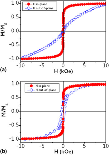
Magnetic hysteresis (M–H) loops measured at room temperature for these two samples using a vibrating sample magnetometer (EG&G model VSM-4500, Oak Ridge, Tennessee) are shown in Figs. 2(a) and 2(b). Magnetization M is normalized to the saturation magnetization M _S, whereas the magnetic field H is applied along different directions relative to the film plane. Clearly, M–H loops depend on the angle of the applied magnetic field relative to film plane and angular distributions of the elongated axis of the particles significantly affect the magnetization processes and the magnetic anisotropy. Different M–H loops are found with magnetic fields applied along different orientations with respect to the film plane. Comparatively to Sample A, which consists of particles with elongated axis distributed in the film plane, Sample B with particles having elongated axes mostly orientated out of the film plane exhibits a magnetization with stronger out-of-plane component. We will focus our attention on the M–H loops of these assemblies of particles in the cases of magnetic field applied perpendicular and parallel to the film plane.

FIG. 2.

M–H loops measured at room temperature for (a) Sample A and (b) Sample B prepared at deposition potentials of −1.0 and −1.1 V versus SCE, respectively.

III. SIMULATION DETAILS AND DISCUSSION

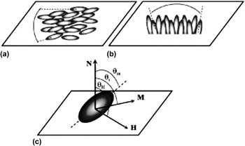
Let us now address our physical assumptions to built a consistent model and perform computational simulations of the M–H loops of these magnetic particle systems. We assume that the samples can be described by systems of ellipsoidal particles for Sample A and half-ellipsoidal particles for Sample B, as shown in Figs. 3(a) and 3(b). The volume of the particles ranges from 5 to 25 µm³ for Sample A and 3 to 50 µm³ for Sample B. A density of 3 × 10⁶ particles per mm² is estimated for sample areas of 20 mm² which are used in magnetic measurements. It is assumed that the magnetic moments inside each particle are quasihomogeneously magnetized and only the total magnetization direction along its easy axis changes from a particle to the next. Every particle i consists of a single magnetic domain in the sense that its atomic magnetic moments rotates coherently and their total magnetic moment µ _i is given by constant absolute value |µ _i | = M _S V _i . Here, V _i is the volume of particle i and M _S is the saturation magnetization with value of M _S = 1100 emu/cm³, that is supposed to be independent of the particle volume. The magnetization of all particles can rotate freely in any direction when one external field is applied because the domain wall is not considered. This model represents the reversible and the irreversible magnetization process as well, since the abrupt changes in the orientation of the magnetization mimic the Barkhausen jumps. In the standard SW model, these jumps can appear when the magnetic field intensity crosses the asteroid shape from inside to outside. ^{Reference Szabó and Iványi19}

FIG. 3.

Schematic illustration of the assemblies of (a) elongated ellipsoids and (b) half-ellipsoids used to model the morphology of the Samples A and B, respectively. (c) Convention used to define the angular coordinates between film normal N and major axis (dashed line) of an ellipsoidal particle, magnetization M and applied field H.

The magnetic anisotropy of each particle is expected to be similar to that of the pure cobalt. Whereas, the first-order magnetocrystalline constant denoted by K ₁ is assumed to be very close to bulk value, K ₂ is free to vary from sample to sample. The shape anisotropy also contributes to the effective values for K ₁ and K ₂ constants. ^{Reference Jamet, Wernsdorfer, Thirion, Dupuis, Melinon and Perez20} The easy axes of each particle are spatially distributed at random in each sample. However, there are experimental evidences indicating preferential angular distributions of the elongated axes either parallel or perpendicular to the normal direction of the film plane, as observed in Figs. 1(a) and 1(b). These axes are assumed as easy axes of magnetization. A small number (no more than 100) of particles were considered to obtain a realistic simulation of the M–H loops. The volumes V _i and orientation of easy axes of magnetization (major axis of particle) used as inputs for the calculations. These parameters were independently extracted from the experimental data shown in Figs. 1(a) and 1(b). For sake of simplicity, we disregard the influence of interparticle dipole–dipole interactions on the global magnetization. The total number of particles was progressively increased from 1 to 100. Although numerical simulation of the magnetization distribution in a system composed of few noninteracting magnetic particles can be seen as a simplified approach, it is striking to realize that a quite good agreement is obtained between simulated curves and experimental results using no more than 100 particles.

The total magnetic energy E _i of each particle i is considered by the sum of three contributions: Zeeman field energy, magnetic anisotropy terms of energy (either due to the shape or the crystalline structure of the particle), and domain nucleation energy. Thus, the density of magnetic free energy for each particle can be written as ^{Reference Paes, Graff, Varalda, Etgens and Mosca21–Reference Hrabovsky, Vanelle, Fert, Yee, Redoules, Sadowski, Kanski and Ilver25} :

(1) $${E_i} = - H \cdot {M_{\rm{S}}} + {K_1}{\sin ^2}\left( {{\theta _i} - {\theta _{{\rm{o}}i}}} \right) + {K_2}{\sin ^4}\left( {{\theta _i} - {\theta _{{\rm{o}}i}}} \right) + {E_{\rm{d}}}\quad {\rm{,}}$$

where H is the applied magnetic field, M _S is the saturation magnetization, K ₁ and K ₂ are the effective first- and second-order anisotropy constants, that include a priori magnetocrystalline anisotropy constants added to shape anisotropy constants, ^{Reference Chen, Pardo and Sanchez22} θ _i is the polar angle that the magnetic moment of i-th particle makes with the film normal [see Fig. 3(a)], θ_oi is the polar angle that the easy axis of the i-th particle makes to the film normal, and E _d is an additional contribution which takes into account the domain nucleation energy which is described below.

In Sample A, the particles are assumed as ellipsoids with variable sizes, whereas in Sample B the particles are taken as half-ellipsoids of variable sizes. Initially, the values of θ_oi are randomly generated by taking random initial values. This allows the determination of the angular distribution of the major axis of the particles from the best agreement between simulated and experimental M–H loops. For simplicity, the exchange interaction between particles is disregarded. ^{Reference Zhang, Zhang, Shen and Kronmuller23} These drastic assumptions are of importance to test the validity of our present calculations by comparison with experimental results.

To simulate the M–H loops for a magnetic field applied along the hard axis, we must take into account that there are maybe some particles with their easy axes oriented parallel to the direction of the applied field. This point is important to solve the so-called Brown paradox which states that, in general, the experimental coercivity is much lower than predicted by the SW model. Based on previous works, ^{Reference Winter, Pascher, Krenn, Liu and Furdyna24,Reference Hrabovsky, Vanelle, Fert, Yee, Redoules, Sadowski, Kanski and Ilver25} an additional energy contribution is used only for the particles with their easy axes orientated parallel to the applied magnetic field which is given by:

(2a) $${E_{\rm{d}}} = - {M_{\rm{S}}}{H_{{\rm{o}}i}}\,\cos \left( {{\theta _{i\left( n \right)}} - {\theta _{i\left( {n - 1} \right)}}} \right)\quad ,$$

where H _oi are free parameters that control the coercive field H _c and θ _i(n) is the angle of the n-th iteration of the calculation of the magnetization contribution for the i-th particle. The H _o parameter can be varied from one direction of application of the field to another due to the demagnetizing factors ^{Reference Skomski, Hadjipanayis and Sellmyer26} which also delimit the values of H _o parameters. This approach leads to quite good simulation results. The distribution of the coercive fields from particle to particle prevents the deduction of a precise evaluation of their collective behavior. However, when the particles have the easy-axis aligned along the out-of-plane direction, we must use instead of Eq. (2a), the following equation:

(2b) $${E_{\rm{d}}} = - {M_{\rm{S}}}{H_{{\rm{o}}i}}\,\sin \left( {{\theta _{i\left( n \right)}} - {\theta _{i\left( {n - 1} \right)}}} \right)\quad {\rm{,}}$$

here, the energy minimization procedure to obtain the magnetization needs a more careful analysis than in SW-like models. Considering that the magnetization value must lead to a stable equilibrium, it should be closer to its previous value. Thus, the energy minimization procedure is performed and compared to the calculated magnetization value obtained for an applied field which is slightly different from the previous one. However, the exact calculation of the equilibrium positions of the magnetization for a given field leads to a large number of coupled equations and free parameters. Thus, it was adopted the following procedure. For a given direction of application of the magnetic field, the n-th particle presents easy-axis along or near such a direction in accordance to Figs. 1(a) and 1(b). To minimize the number of parameters is imposed a criterion that H _o values are constant for a given field direction; i.e., there is no angular dependence of this term relative to the applied field direction.

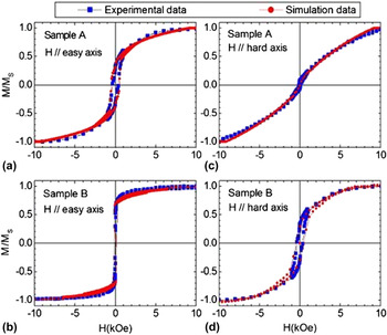
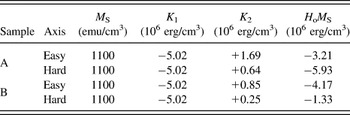
To validate the model were simulate the M–H loops measured at room temperature for Sample A and Sample B with magnetic field applied parallel and perpendicular to film plane. MC simulations were used to calculate the magnetization of the particles in the applied magnetic field for each easy axis configuration of magnetization. The representative number of particles was increased up to 100 to obtain reasonable simulations of the magnetic hysteresis loops. In these simulations considering assemblies of N × N particles with N = 10 were left free to vary only with the values of second-order anisotropy constant, K ₂, and the parameter that controls the coercivity for the assembly of particles, namely H _o. All others parameters were kept fixed, independent of the orientation of the applied magnetic field relative to film plane. MC simulations are shown in Fig. 4 only with N = 10. Simulated and measured M–H loops for magnetic field applied along the in-plane easy axes of magnetization for Sample A and Sample B are shown in Figs. 4(a) and 4(b), respectively. A good agreement is obtained between simulations and experimental results for both samples, including reasonable values for coercivities and remanences. Our simulations of the M–H loops with magnetic field applied along the hard axis of magnetization of Sample A and Sample B are shown in Figs. 4(c) and 4(d), respectively. Again, these simulations are in good agreement with experimental data. The values used in these simulations are given in Table I. For magnetic field applied in the easy axis, both M _S and K ₁ are the same for Samples A and B. Different values for K ₂ and H _o M _S were used to obtain the simulations of hysteresis loops observed for Sample A and Sample B. The same M _S and K ₁ values were used for magnetic field applied along the hard axis. Again, the hysteresis loops for Sample A and Sample B are better reproduced using different values for K ₂ and H _o M _S. Such changes in K ₂ and H _o are expected because the contribution of shape anisotropy is included in the K ₂ anisotropy constant and H _o values. These values depend on the average major axis of the particles along the applied field direction.

FIG. 4.

Simulated (red filled circles) and experimental (blue filled squares) M–H loops for Sample A and Sample B with magnetic field applied along the easy magnetic axes in the film plane (a and b) and hard magnetic axes perpendicular to the film plane (c and d).

TABLE I.

Magnetic parameters resulting from the MC simulations of magnetic hysteresis.

According to the simulations for Sample A, the easy axes of magnetization are aligned parallel to the film normal for 6% of the particles. For the remaining 94% of the particles, the easy axes of magnetization exhibit azimuthal angles randomly oriented in the film plane and polar angles ranging in between 45° and 90° (in the film plane). For Sample B, the simulations correspond to 40% of the particles with easy axes of magnetization aligned along the film normal and the remainder particles present a distribution of the easy axis of magnetization centered at 0° with an angular opening of 45° and a width of approximately 26°. These features are in good agreement with the features of SEM images shown in Figs. 1(a) and 1(b). Therefore, reasonable simulation results are generated using realistic size distributions and angular distributions of easy axes of magnetization.

In our simulations, the values of M _S and K ₁ are kept constant and quite close to values found for bulk Co. It is noticed that the minus signal of K ₁ results from the polar angle definition with respect to the film plane in our measurements. Despite the intervention of the shape anisotropy constants, K ₂ values resulting from simulations are also quite reasonable if compared to values reported for bulk Co. In a certain way, it is therefore surprising that the reasonable simulations of the experimental results were obtained using a modified-SW model and considering a relatively small number of particles without dipole–dipole interactions and interparticle exchange coupling. A possible explanation to successful MC simulations is that coherent rotation of magnetization and quite uniform switching field are in fact predominant mechanisms. Furthermore, it is likely that dipole–dipole interactions have weak effective strength and conformation of the particles creates a spatial variation of the local magnetic properties, such that the intrinsic shape anisotropy and coercivity of each particle becomes efficient enough to break the interactions between particles. ^{Reference Zhang, Zhang, Shen and Kronmuller23} The idea of introducing the magnetic dipolar interaction within an extension of the SW model is a very appealing goal, but very difficult indeed since the dipolar interaction is highly nonlinear. Also, the energy minimization procedure to calculate the magnetization for an applied field becomes much more complex if is taken into account the dipole–dipole interaction between particles. Dipolar interaction between particles can be made using the expression:

(3) $${E_{{\rm{dip}}}} = \sum\limits_{i \ne j} {\left( {{{{{\rm{\mu }}_i} \cdot {{\rm{\mu }}_j}} \mathord{\left/ {\vphantom {{{{\rm{\mu }}_i} \cdot {{\rm{\mu }}_j}} {\mathop {{r_{ij}}}\nolimits^3 - 3{{\left( {{{\rm{\mu }}_i} \cdot {r_{ij}}} \right)\left( {{{\rm{\mu }}_j} \cdot {r_{ij}}} \right)} \mathord{\left/ {\vphantom {{\left( {{{\rm{\mu }}_i} \cdot {r_{ij}}} \right)\left( {{{\rm{\mu }}_j} \cdot {r_{ij}}} \right)} {\mathop {{r_{ij}}}\nolimits^5 }}} \right. \kern-\nulldelimiterspace} {\mathop {{r_{ij}}}\nolimits^5 }}}}} \right. \kern-\nulldelimiterspace} {\mathop {{r_{ij}}}\nolimits^3 - 3{{\left( {{{\rm{\mu }}_i} \cdot {r_{ij}}} \right)\left( {{{\rm{\mu }}_j} \cdot {r_{ij}}} \right)} \mathord{\left/ {\vphantom {{\left( {{{\rm{\mu }}_i} \cdot {r_{ij}}} \right)\left( {{{\rm{\mu }}_j} \cdot {r_{ij}}} \right)} {\mathop {{r_{ij}}}\nolimits^5 }}} \right. \kern-\nulldelimiterspace} {\mathop {{r_{ij}}}\nolimits^5 }}}}} \right)}\quad ,$$

where µ _i and µ _j are the magnetic moment of the particles at sites i or j and r _ij = |r _ij | is the distance between the centers of the particles. It is worth noticing that magnetic dipole–dipole interactions are directional, repulsive, or attractive depending on the relative orientation of the dipoles in the space. The dipolar energy density decays as the inverse cube of the distance between particles and scales linearly with volume of the particle. Taking the average values of particle volumes and interparticle distances, one can estimate an average dipolar energy per unit volume not exceeding U (= 〈E _dip/V _i 〉) ∼ 2 × 10⁶ erg/cm³. Therefore, the ratio U/|K ₁| ∼ 0.4 indicates an average dipolar interaction smaller than the first-order effective anisotropy term. Another magnetic interaction disregarded in our simulations is the interparticle exchange coupling which predominates when the ratio of surface area to volume increases with decreasing particle size. ^{Reference Zhang, Zhang, Shen and Kronmuller23} Also, the interparticle exchange coupling depends on the imperfections of particle boundaries and it generally results in a decrease of exchange coupling with the disconnection of the particles. ^{Reference Zhang, Zhang, Shen and Kronmuller23} Therefore, different sizes and shapes of particles, together with coercive mechanism related with spatial distribution of magnetization easy axes, contributing to the magnetic interactions play a minor role in both samples. Comparison with experimental data justifies our calculations with only a few realistic magnetic parameters.