





1. Introduction
Accelerating technological change is essential to the societal transformations needed for climate mitigation and sustainable development (Sharpe, Reference Sharpe2023). Renewable electricity technologies such as wind and solar power have been expanding rapidly, yet not nearly fast enough to deliver the deep cuts in emissions required over the coming decade (IEA, 2021; IRENA, 2024b; Suzuki et al., Reference Suzuki, Jewell and Cherp2023). The hope that the necessary acceleration will nevertheless materialize rests on two premises. The first is the common ‘S-curve’ model of technology diffusion and the related concept of positive tipping points in technological change: once a technology matures, self-reinforcing feedbacks are expected to propel continued acceleration until saturation is approached (Lenton et al., Reference Lenton, Milkoreit, Willcock, Abrams, Armstrong McKay, Buxton, Donges, Loriani, Wunderling, Alkemade, Barrett, Constantino, Powell, Smith, Boulton, Dennis, Dijkstra, Pearce-Kelly, Pinho and Roman-Cuesta2025; Mey et al., Reference Mey, Mangalagiu and Lilliestam2024; Nijsse et al., Reference Nijsse, Mercure, Ameli, Larosa, Kothari, Rickman, Vercoulen and Pollitt2023). The second is that stronger policies – adopted in response to intensifying climate concerns and, more recently, to energy security pressures – will push growth beyond what market dynamics alone would deliver (Sovacool et al., Reference Sovacool, Geels, Andersen, Grubb, Jordan, Kern, Kivimaa, Lockwood, Markard, Meadowcroft, Meckling, Moore, Raven, Rogge, Rosenbloom, Schmidt, Schot, Sharp, Stephenson, Vormedal and Yang2025).
However, empirically, slowing and even stagnating growth of renewable technologies are common (Cherp et al., Reference Cherp, Vinichenko, Tosun, Gordon and Jewell2021; Jewell et al., Reference Jewell, Cherp, Geels, Suzuki, Nacke, Tosun, Bhowmik, Kazlou, Jakhmola and Vinichenko2026). Nor do policies always deliver the expected boost: political setbacks – from shifting governing coalitions to organized opposition – frequently derail more ambitious measures (Markard, Reference Markard2018; Stokes, Reference Stokes2020), while even well-designed schemes run up against limits in public finance, administrative capacity, and social acceptance (Boasson et al., Reference Boasson, Peters and Tosun2025; Sovacool et al., Reference Sovacool, Geels, Andersen, Grubb, Jordan, Kern, Kivimaa, Lockwood, Markard, Meadowcroft, Meckling, Moore, Raven, Rogge, Rosenbloom, Schmidt, Schot, Sharp, Stephenson, Vormedal and Yang2025). Reflecting on these obstacles, recent transitions literature suggests that acceleration may be limited to only early phases of transition, after which near-linear growth at a high but stable speed can be expected (Jewell et al., Reference Jewell, Cherp, Geels, Suzuki, Nacke, Tosun, Bhowmik, Kazlou, Jakhmola and Vinichenko2026; Sovacool et al., Reference Sovacool, Geels, Andersen, Grubb, Jordan, Kern, Kivimaa, Lockwood, Markard, Meadowcroft, Meckling, Moore, Raven, Rogge, Rosenbloom, Schmidt, Schot, Sharp, Stephenson, Vormedal and Yang2025). Yet little systematic research has traced the actual shape and parameters of deployment trajectories of policy-driven technologies or linked turning points to specific policy interventions. We ask whether these trajectories differ from standard diffusion expectations and whether the differences are linked to policy shifts.
We address this question by analyzing the four decades of onshore wind power growth in European Union (EU) countries. Wind supplies a higherer share of electricit in the EU than in any other major economy; its deployment accelerated strongly in the 1990s and 2000s, but has remained largely flat over the last 15 years. Many national and EU-level targets now call for reacceleration, including a doubling of installed capacity by 2030 (European Commission, 2022; Pavlenko & Cherp, Reference Pavlenko and Cherp2026), which signals strong policy involvement. To conduct our analysis, we introduce a model for identifying turning points in growth trajectories as well as new metrics for measuring growth. We map growth peaks and turning points against policy shifts and also evaluate whether the 2030 policy targets and deployment forecasts fall within or exceed the growth rates that countries have historically achieved.
Our analysis shows that, contrary to positive tipping point theories, the initial acceleration of wind power has ended in most countries, and that this occurred much earlier than common S-curve theories expect: already when wind reached about 2% of its capacity potential (IQR 1–4%) or generated 4% of electricity (IQR 1.5–6%). In most countries, these first slowdowns closely followed the capping, withdrawal, or destabilization of financial supporting policies. Yet the first peaks were not the beginning of terminal stagnation: growth typically reaccelerated through secondary and sometimes tertiary growth pulses. Before 2020, this reacceleration was again led by policy changes, and starting from 2021, also by market dynamics: rising electricity prices and low technology costs. In both periods, the peak growth rates at subsequent pulses were statistically close to first-peak rates, pointing to persistent constraints such as fiscal capacity, permitting throughput, and social acceptance. The aggregate effect of these pulses has been a remarkably stable average rate of annual additions – ‘cruising speed’ (Jakhmola et al., Reference Jakhmola, Jewell, Vinichenko and Cherp2026b; Jewell et al., Reference Jewell, Cherp, Geels, Suzuki, Nacke, Tosun, Bhowmik, Kazlou, Jakhmola and Vinichenko2026) – at roughly one-quarter below the first-pulse peak. Recent targets adopted in response to heightened climate and energy security pressures require growth close to historical peaks, but forecasted growth falls below these targets and reverts to the cruising speed. Policy-driven acceleration of mature technologies therefore appears to be bounded by persistent limits that may be difficult to surpass. Our data-driven approach – combining the identification of turning points, measuring growth rates, and policy analysis – can be applied to other technologies to generate ‘stylized facts’ essential for bridging mathematical modeling and mechanism-based explanations of technological change (Geels et al., Reference Geels, Berkhout and van Vuuren2016; Trutnevyte et al., Reference Trutnevyte, Hirt, Bauer, Cherp, Hawkes, Edelenbosch, Pedde and Van Vuuren2019).
2. State of knowledge and theoretical framework
Technology diffusion literature commonly describes the growth of new technologies as an S-shaped trajectory: initially slow growth accelerates and then slows down (Griliches, Reference Griliches1957; Grübler et al., Reference Grübler, Nakićenović and Victor1999). This pattern tracks the empirical reality of historical technologies and also captures two fundamental mechanisms governing diffusion. First, technology growth is driven by ‘increasing returns’ (Arthur, Reference Arthur1994) or positive feedback loops, the most prominent of them being cost decline through learning and economies of scale, whereby greater deployment reduces costs and thus stimulates further adoption (Lafond et al., Reference Lafond, Bailey, Bakker, Rebois, Zadourian, McSharry and Farmer2018; Way et al., Reference Way, Ives, Mealy and Farmer2022; Wright, Reference Wright1936). This mechanism underpins the early stage of the S-curve. Second, diffusion ultimately encounters finite market size or geophysical constraints, which impose a negative feedback that slows growth at later stages (Cherp et al., Reference Cherp, Vinichenko, Tosun, Gordon and Jewell2021; Rao & Kishore, Reference Rao and Kishore2010). A key feature of both mechanisms is their monotonic dependence on deployment: costs progressively decline while untapped market potential is progressively depleted. Together, these dynamics yield a trajectory with a single inflection point – the moment at which positive and negative feedbacks balance, the growth rate peaks and then begins to decline (Cherp et al., Reference Cherp, Vinichenko, Tosun, Gordon and Jewell2021). The logistic function, which formalizes this process by placing the inflection point at the midpoint of the deployment ceiling, has been the canonical model in the technology diffusion literature (Grubb et al., Reference Grubb, Drummond, Ives, Farmer and Kelkar2021; Grubler & Nakicenovic, Reference Grubler and Nakicenovic1991; Marchetti & Nakicenovic, Reference Marchetti and Nakicenovic1979; Wilson et al., Reference Wilson, Grubler, Bauer, Krey and Riahi2013).
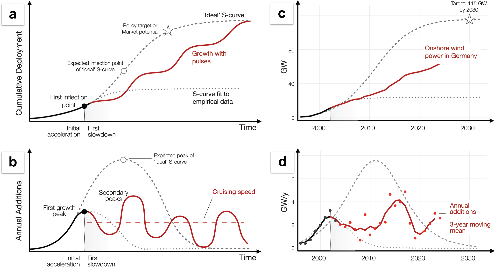
However, this framework struggles to explain and predict the growth of renewable power. The main explanatory variable in the S-curve model is the technology’s position with respect to the inflection point (Baumgärtner et al., Reference Baumgärtner, Way, Ives and Farmer2024; Cherp et al., Reference Cherp, Vinichenko, Tosun, Gordon and Jewell2021; Jakhmola et al., Reference Jakhmola, Jewell, Vinichenko and Cherp2026b; Way et al., Reference Way, Ives, Mealy and Farmer2022), yet this is difficult to determine for technologies that are still expanding (dotted curves on Figure 1). Interpreting an observed growth peak as the ‘true’ inflection point tends to under-predict future deployment (Baumgärtner et al., Reference Baumgärtner, Way, Ives and Farmer2024; Madsen & Hansen, Reference Madsen and Hansen2019; Rypdal, Reference Rypdal2018), whereas inferring an inflection point based on assumed market potential or policy targets (Grubb et al., Reference Grubb, Drummond, Ives, Farmer and Kelkar2021; Way et al., Reference Way, Ives, Mealy and Farmer2022) tends to overestimate it (long-dash curve on Figure 1d). This problem reflects a deeper issue: the canonical diffusion model does not fully account for technologies whose expansion depends heavily on policy support, as is the case for renewable energy (Kulmer et al., Reference Kulmer, Seebauer, Hinterreither, Kortschak, Theurl and Haas2022; Rao & Kishore, Reference Rao and Kishore2010; Schmidt & Sewerin, Reference Schmidt and Sewerin2017). For such policy-driven technologies, growth is shaped not only by learning and market access, but also by the availability, design, and stability of policy instruments, including feed-in tariffs (FiTs), auctions, and planning regulations. These political drivers introduce their own feedback. Deployment can generate supportive constituencies that reinforce policy ambition (‘ratcheting up’) (Meckling et al., Reference Meckling, Lipscy, Finnegan and Metz2022; Pahle et al., Reference Pahle, Burtraw, Flachsland, Kelsey, Biber, Meckling, Edenhofer and Zysman2018), but it can also provoke backlash through rising fiscal costs, distributional conflicts, local opposition, or shifting political priorities (Markard, Reference Markard2018; Stokes, Reference Stokes2020). Moreover, policymakers may respond adaptively to emerging barriers or opportunities, introducing new interventions that reshape diffusion trajectories (Jewell et al., Reference Jewell, Cherp, Geels, Suzuki, Nacke, Tosun, Bhowmik, Kazlou, Jakhmola and Vinichenko2026). Crucially, these feedbacks do not necessarily evolve in sync with the technological dynamics underpinning the S-curve.
Growth of policy-driven technologies with multiple pulses and stable cruising speed deviates from standard S-curve models.

Figure 1 Long description
The figure has four panels arranged in a two-by-two grid. Panels A and B are conceptual diagrams. Panels C and D apply the same comparison to onshore wind power in Germany. In all panels, black and grey elements represent the idealized S-curve pattern, while red elements represent growth with pulses or observed German onshore wind deployment. Panel A plots cumulative deployment on the vertical axis against time on the horizontal axis. A black curve rises slowly at first and then reaches a first inflection point, shown with a black dot. After this point, two “ideal” S-curves are shown. A dotted curve labeled “S-curve fit to empirical data” starts to decline following the first inflection point and peaks relatively early. While the dashed S-curve continues upward after the first inflection point toward a “Policy target or market potential” marked by a star on the figure. A red curve labeled “Growth with pulses” also departs from the first inflection point, but instead of following a smooth S-shape, it increases in several pulses: rapid growth periods separated by slower growth periods. Panel B plots annual additions on the vertical axis against time on the horizontal axis. A black curve rises to a first growth peak, marked with a black dot. The grey dotted “S-curve fit to empirical data” shows a single early peak and then declines toward near-zero annual additions after that peak. The grey dashed “ideal” S-curve forms larger bell-shaped curve with a later peak, before declining toward zero. The red pulse-based trajectory instead shows multiple peaks and troughs: it falls after the first growth peak, rises to a higher secondary peak, drops again, and then continues with repeated smaller waves. A red horizontal dashed line labeled “Cruising speed” indicates an approximate long-term average level around which the later red waves fluctuate. Panel C plots cumulative onshore wind power in Germany in gigawatts from about 2000 to 2030. The red line shows observed cumulative deployment, rising from near zero around 2000 to roughly the mid-50 GW range by the early 2020s in a stepwise pattern with alternating faster and slower growth. The grey dotted “S-curve fit to empirical data” stays well below the observed trajectory and levels off around the mid-20 GW range. The grey dashed “ideal” S-curve rises much more steeply after the early 2000s and continues toward a star labeled “Target: 115 GW by 2030”. Panel D plots annual onshore wind additions in Germany in gigawatts per year from about 2000 to 2030. Black and red points show annual additions, and a red line shows the three-year moving mean. The observed annual additions rise from below 1 GW per year around 2000 to an early peak of around 2 to 3 GW per year in the early 2000s, then decline and fluctuate at lower levels through the late 2000s. They rise again in the mid-2010s to around 4 to 5 GW per year, drop sharply around 2019, and then recover to around 2 to 3 GW per year in the early 2020s. The grey dotted “S-curve fit to empirical data” shows a single early peak and then declines toward near-zero annual additions. The grey dashed “ideal” S-curve forms one large bell-shaped peak, reaching above 6 GW per year around the early 2010s before declining toward near-zero by 2030.
Whether and how political forces affect S-shaped trajectories depends on both the timing of policy interventions and their strength relative to non-policy diffusion mechanisms. With respect to timing, if policy dynamics broadly align with technological forces so that increasing political returns reinforce the positive feedbacks from learning and scale, while political backlash coincides with tightening market constraints – single-inflection S-curves may still provide a reasonable approximation. Cherp et al. (Reference Cherp, Vinichenko, Tosun, Gordon and Jewell2021) implicitly adopt this view, assuming that technological and political feedbacks balance contemporaneously, giving rise to a ‘stable growth phase’ around the inflection point. Jewell et al. (Reference Jewell, Cherp, Geels, Suzuki, Nacke, Tosun, Bhowmik, Kazlou, Jakhmola and Vinichenko2026) further develop this mechanism, describing how a ‘steady growth phase’ can be sustained by policies that respond to emerging socio-technical barriers, thereby maintaining a balance between drivers and constraints and preventing premature slowdown before policy goals are reached. However, policy dynamics may also follow their own internal logic – shaped by electoral cycles, fiscal pressures, or geopolitical shocks – operating on timescales that are not synchronized with technological change. In such cases, political feedbacks are more likely to reshape standard diffusion trajectories. The magnitude of this effect also depends on the relative importance of policies vis-à-vis other factors: in contexts where renewables rely heavily on policy support, their trajectories are more strongly shaped by political change than in markets where they are already commercially competitive.
When policy interventions are both essential and not synchronized with technological evolution, they can interfere with the gradual, monotonic forces of cost decline and market saturation, producing qualitatively different growth paths (Figure 1). First, the slowdown following the first inflection point may occur not when a technology approaches half of its market potential, but when the policy support underpinning early growth is weakened, withdrawn, or destabilized. In such cases, the first inflection point reflects the limits of the initial policy regime rather than underlying market or geophysical constraints. Second, this initial growth peak does not necessarily mark the onset of sustained deceleration. Because policy regimes can be reformed, strengthened, or reinstated, growth may reaccelerate, producing multiple growth pulses rather than a single transition from acceleration to slowdown. Kulmer et al. (Reference Kulmer, Kortschak, Seebauer, Zachariadis, Milne and Andersen2020, Reference Kulmer, Seebauer, Hinterreither, Kortschak, Theurl and Haas2022) identified turning points in the deployment of electric vehicles, heat pumps, and solar PV in Austria and linked them to policy and technology changes. Cherp et al. (Reference Cherp, Vinichenko, Tosun, Gordon and Jewell2021) detected surprisingly early inflection points in most countries and identified pulses in solar and wind deployment in several countries, but still used standard S-curve models for their analysis. Similarly, Baumgärtner et al. (Reference Baumgärtner, Way, Ives and Farmer2024) considered ‘periods of acceleration and deceleration’ as fluctuations of canonical S-curves. Vetier et al. (Reference Vetier, Pavlenko, Jewell and Cherp2024) discussed wind power growth pulses in European countries, arguing that they are caused by policy shifts and comparing growth rates at the initial and subsequent pulses. Jakhmola et al. (Reference Jakhmola, Jewell, Vinichenko and Cherp2026a) provided additional evidence for pulses of wind and solar power by demonstrating that the bi-logistic growth model (a combination of two logistic curves) can often capture deployment trajectories better than a standard logistic model. Jewell et al. (Reference Jewell, Cherp, Geels, Suzuki, Nacke, Tosun, Bhowmik, Kazlou, Jakhmola and Vinichenko2026) argued that pulses are common and arise from the shifting balance of barriers and drivers. Despite these advances, the prevalence, drivers, and statistical properties of pulses and turning points remain largely unexplored. It is in particular not clear what typical pulses are, whether peak growth rate changes or stays the same across pulses, and whether pulses arise from socio-technical phenomena, autonomous policy shifts, or coupled policy-technology dynamics.
Systematically investigating the prevalence and characteristics of growth pulses requires tools and metrics that are different from standard S-curve models. These tools should be able to diagnose distinct growth segments with different patterns of growth. Such patterns are most visible on charts of annual capacity additions where an S-curve appears as an inverted U-shape, with the inflection point at the peak where the growth is fastest; see Figures 1 and 2. A growth trajectory with more than one inflection point would have more than one growth pulse separated by turning points, and a linear growth would be represented by a horizontal line. In addition to diagnostic tools, we use new growth metrics: peak growth rate, the maximum rate achieved at the inflection point of each pulse, and cruising speed (Jakhmola et al., Reference Jakhmola, Jewell, Vinichenko and Cherp2026b; Jewell et al., Reference Jewell, Cherp, Geels, Suzuki, Nacke, Tosun, Bhowmik, Kazlou, Jakhmola and Vinichenko2026), the average of annual additions after the first peak. Mapping the pulses onto policy shifts under different market conditions and comparing growth rates with policy targets advances the understanding of policy-driven acceleration of transition. Our approach and methods are discussed in more detail in the following section.
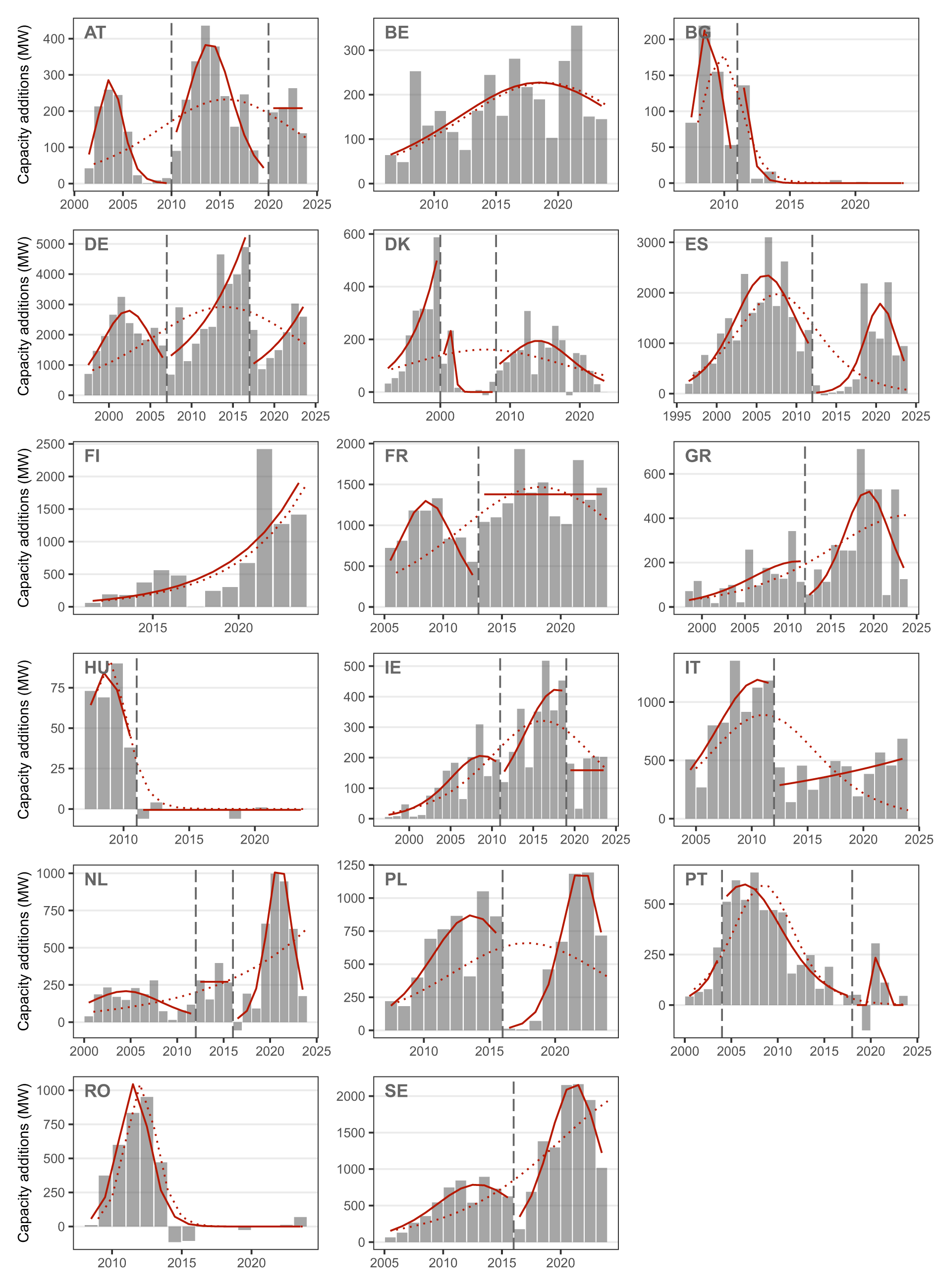
Annual additions of onshore wind capacity in 17 European countries with growth segments and turning points; Czechia is omitted because wind power has not yet taken off.

Figure 2 Long description
The figure is a grid of 17 small charts showing annual onshore wind capacity additions in 17 European countries. The horizontal axis in each panel shows years, generally from the late 1990s or early 2000s to the early 2020s, although the exact start year differs by country. The vertical axis shows annual capacity additions in megawatts. The vertical scales differ between panels: Germany and Spain reach several thousand megawatts per year, while smaller markets such as Hungary, Bulgaria, and Austria remain below a few hundred megawatts per year. Grey vertical bars represent observed yearly capacity additions. Solid red curves show fitted growth pulses. Dotted red curves show single S-curves fitted to each country’s whole data series. Vertical dashed lines mark turning points between pulses. Austria shows three pulses. The first runs from 2001 to 2010, peaking in 2004 (285 MW). A turning point occurs in 2010. The second runs from 2010 to 2020, peaking in 2014 (382 MW). A second turning point occurs in 2020. The third runs from 2020 to 2024, with its maximum in 2020 (208 MW). Belgium has one pulse, running from 2006 to 2024 and peaking in 2019 (227 MW). No turning point is identified. Bulgaria shows two pulses. The first runs from 2007 to 2011, peaking in 2009 (155 MW). A turning point occurs in 2011. The second runs from 2011 to 2024, with its maximum in 2011 (53 MW), followed by declining additions. Germany shows three pulses. The first runs from 1997 to 2007, peaking in 2003 (2,792 MW). A turning point occurs in 2007. The second runs from 2007 to 2017, peaking in 2017 (5,213 MW). A second turning point occurs in 2017. The third runs from 2017 to 2024, peaking in 2024 (2,920 MW). Denmark shows three pulses. The first runs from 1992 to 2000, peaking in 2000 (499 MW). A turning point occurs in 2000. The second runs from 2000 to 2008, peaking in 2001 (135 MW). A second turning point occurs in 2008. The third runs from 2008 to 2024, peaking in 2015 (194 MW).Spain shows two pulses. The first runs from 1996 to 2012, peaking in 2007 (2,341 MW). A turning point occurs in 2012. The second runs from 2012 to 2024, peaking in 2021 (1,783 MW). Finland shows one pulse, running from 2011 to 2024 and peaking in 2024 (1,900 MW). No turning point is identified. France shows two pulses. The first runs from 2005 to 2013, peaking in 2009 (1,298 MW). A turning point occurs in 2013. The second runs from 2013 to 2024, with its maximum in 2013 (1,380 MW). Greece shows two pulses. The first runs from 1998 to 2012, peaking in 2012 (206 MW). A turning point occurs in 2012. The second runs from 2012 to 2024, peaking in 2020 (520 MW). Hungary shows one pulse, running from 2007 to 2011 and peaking in 2009 (84 MW). A turning point occurs in 2011. This is followed by a non-pulse segment from 2011 to 2024, with little or no deployment. Ireland shows three pulses. The first runs from 1997 to 2011, peaking in 2009 (206 MW). A turning point occurs in 2011. The second runs from 2011 to 2019, peaking in 2018 (422 MW). A second turning point occurs in 2019. The third runs from 2019 to 2024, with its maximum in 2019 (159 MW). Italy shows two pulses. The first runs from 2004 to 2012, peaking in 2011 (1,191 MW). A turning point occurs in 2012. The second runs from 2012 to 2024, peaking in 2024 (514 MW). The Netherlands shows three pulses. The first runs from 2000 to 2012, peaking in 2005 (208 MW). A turning point occurs in 2012. The second runs from 2012 to 2016, with its maximum in 2012 (271 MW). A second turning point occurs in 2016. The third runs from 2016 to 2024, peaking in 2021 (1,005 MW). Poland shows two pulses. The first runs from 2007 to 2016, peaking in 2014 (869 MW). A turning point occurs in 2016. The second runs from 2016 to 2024, peaking in 2022 (1,170 MW). Portugal shows three pulses. The first runs from 2000 to 2004, peaking in 2004 (221 MW). A turning point occurs in 2004. The second runs from 2004 to 2018, peaking in 2007 (597 MW). A second turning point occurs in 2018. The third runs from 2018 to 2024, peaking in 2021 (120 MW). Romania shows one pulse, running from 2008 to 2024 and peaking in 2012 (1,045 MW). Additions subsequently decline to near zero, but no turning point is identified. Sweden shows two pulses. The first runs from 2005 to 2016, peaking in 2013 (785 MW). A turning point occurs in 2016. The second runs from 2016 to 2024, peaking in 2022 (2,152 MW).
3. Methodology
3.1. Scope of analysis
We focus on onshore wind energy in the EU: a mature technology in a region with high deployment and pronounced national-level variation. Commercial onshore wind power in the EU originated in the 1980s (Gipe & Möllerström, Reference Gipe and Möllerström2023) and currently supplies around 15% of electricity generation (Ember, 2026), the highest share among major global economies. We analyze onshore wind in the 18 largest EU member states (those with total electricity generation  $ \gt $30 TWh in 2024), excluding smaller countries where individual projects can cause large fluctuations (Cherp et al., Reference Cherp, Vinichenko, Tosun, Gordon and Jewell2021) (see Supplementary Table S1 for the full list). We use historical data from 1992 onwards on installed capacity, generation, and total electricity supply from IEA (2025a), IRENA (2025), and Eurostat (2025).
Our analysis proceeds in four stages: diagnosing growth pulses from multi-segment model fitting, testing whether pulses are synchronized across countries, measuring and normalizing growth rates, and analyzing the role of policy shifts.
3.2. Diagnosing turning points and measuring growth
We build on the tradition of fitting growth models to empirical time series (Cherp et al., Reference Cherp, Vinichenko, Tosun, Gordon and Jewell2021; Griliches, Reference Griliches1957; Grubler & Nakicenovic, Reference Grubler and Nakicenovic1991; Wilson et al., Reference Wilson, Grubler, Bauer, Krey and Riahi2013), advancing the algorithm of Kulmer et al. (Reference Kulmer, Seebauer, Hinterreither, Kortschak, Theurl and Haas2022) for identifying significant changes in growth trajectories. We introduce the multi-segment growth model and inflection point algorithm because this method excels at detecting subtle shifts between growth regimes (Jewell et al., Reference Jewell, Cherp, Geels, Suzuki, Nacke, Tosun, Bhowmik, Kazlou, Jakhmola and Vinichenko2026). Our method involves three steps.
3.2.1. Filtering out early datapoints
We start the data series for each country 3 years before the technology ‘takeoff’, when wind power generation first exceeds 1% of the total electricity supply (Cherp et al., Reference Cherp, Vinichenko, Tosun, Gordon and Jewell2021), but not earlier than 1992 in order to exclude Denmark’s atypical pre-1992 deployment (Meyer, Reference Meyer1995).
3.2.2. Fitting multi-segment growth models
Following Kulmer et al. (Reference Kulmer, Kortschak, Seebauer, Zachariadis, Milne and Andersen2020, Reference Kulmer, Seebauer, Hinterreither, Kortschak, Theurl and Haas2022) with modifications, we build compound growth models comprising multiple logistic and linear segments (Figure S1 and Equations 1–3 in Supplementary Note S1). To avoid overfitting, each segment must be at least 4 years long – enough datapoints for meaningful parameter estimation while still capturing policy-relevant growth episodes (Kulmer et al., Reference Kulmer, Seebauer, Hinterreither, Kortschak, Theurl and Haas2022; Wilson et al., Reference Wilson, Grubler, Bauer, Krey and Riahi2013). We fit all possible combinations of turning points and segment functions using the 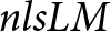 $nlsLM$ function from the
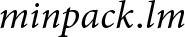 $minpack.lm$ package in R. For example, for Germany (28 datapoints, 1997–2024), this yields 3,497 candidate models.
3.2.3. Selecting the best-performing model
We select the best model using a modified version (‘mAIC’) of the corrected Akaike information criterion (Akaike, Reference Akaike1974; Hurvich & Tsai, Reference Hurvich and Tsai1989), which penalizes extra parameters and, additionally, extra curve segments to prevent overfitting (Equation 4 in Supplementary Note S1). We tested a range of penalty strengths for the mAIC criterion and selected the k = 3 value that best matched the identified segments to the observed annual capacity additions across all countries. The best model for Germany, for instance, has three logistic segments separated by turning points in 2007 and 2017 (Figure 2).
3.3. Testing whether pulses are synchronized across countries
To test whether the timing of growth peaks was synchronized across countries, which would suggest shared European or global drivers rather than purely national-level mechanisms, we compared the observed distribution of peak years with an exposure-adjusted Monte Carlo null model. In the null model, the total number of observed peaks was held fixed, but peaks were randomly redistributed across years with probabilities proportional to the number of countries observed in each year. This accounts for variation in country-year coverage over time. We applied the same test separately to turning-point years.
3.4. Measuring and normalizing growth rates
For each segment, we calculate the maximum (peak) growth rate from the fitted model (Figure S1). For linear segments, this is constant; for logistic segments, the peak rate depends on whether the inflection point falls within the segment and on the growth duration of the fitted curve (Equation 5 in Supplementary Note S1). When the inflection point lies within the segment and growth duration exceeds 3 years, we use the rate at the inflection point (Cherp et al., Reference Cherp, Vinichenko, Tosun, Gordon and Jewell2021; Wilson et al., Reference Wilson, Grubler, Bauer, Krey and Riahi2013); when growth duration is shorter, we use the maximum average 3-year rate (Cherp et al., Reference Cherp, Vinichenko, Tosun, Gordon and Jewell2021; Vinichenko et al., Reference Vinichenko, Jewell, Jacobsson and Cherp2023; Wilson et al., Reference Wilson, Grubler, Bauer, Krey and Riahi2013); when the inflection point lies outside the segment, we use the maximum rate achieved within it (see Panel A of Figure S1). We measure the cruising speed as the average annual capacity additions between the first inflection point and the end of the data series.
We measure target and forecast growth rates by taking the difference between the 2030 target or forecast and installed capacity at the end of 2024, divided by 6 years. Policy targets for onshore wind capacity in 2030 are derived from the most recent National Energy and Climate Plans (NECPs) (European Commission, 2025). Where NECPs specified targets in generation rather than capacity, we converted using the last 3 years’ average national capacity factor; where targets combined onshore and offshore wind, we consulted additional national and EU documents to isolate onshore values (Supplementary Table S1). Forecasts for 2030 are taken from WindEurope (WindEurope, 2026) and for sensitivity analysis also from IEA (IEA, 2025b). WindEurope (2026) provides consistent country-level estimates across all countries in our sample based on the project pipeline, permitting data, and auction volumes.
We normalize all growth rates for inter-country comparisons. Previous studies normalized by total electricity supply (Cherp et al., Reference Cherp, Vinichenko, Tosun, Gordon and Jewell2021; Vinichenko et al., Reference Vinichenko, Jewell, Jacobsson and Cherp2023), but this does not capture spatial constraints such as land availability (Kohsaka & Kohyama, Reference Kohsaka and Kohyama2023) or changing electricity demand. We therefore additionally normalize by capacity potential – the estimated maximum installable wind capacity per country, using the median estimate from (Dupré la Tour, Reference Dupré la Tour2023).
3.5. Policy analysis
We analyzed the relationship between policy shifts and wind power growth at two levels. First, we identified the timing of each pulse's initial acceleration, its peak and subsequent reaccelerations (Table S2), distinguishing reaccelerations peaking before and after 2021 – when rapidly rising electricity prices (IEA, 2022) combined with the preceding decade of cost reductions (IRENA, 2024a) brought onshore wind close to grid parity (Batz Liñeiro & Müsgens, Reference Batz Liñeiro and Müsgens2025; Enervis, 2022), potentially changing the role of state support. These events were mapped against policy shifts (introduction, expansion, cut, or switch of financial support instruments) documented in Council of European Energy Regulators (CEER) reports 2004–2025 (Supplementary Note S2, Section A). Second, we conducted detailed case studies of Austria, Denmark, Poland, and Spain – selected via a combination of extreme-case and diversity sampling (Patton, Reference Patton2002) for their pronounced stalling episodes, geographic spread, and coverage of the main EU support-instrument types. For each, we traced the causal mechanism from policy change to deployment outcome, drawing on regulatory documents, industry reports, and country-specific literature (Supplementary Note S2, Section B).
4. Results
4.1. Wind power trajectories deviate from classic S-curves
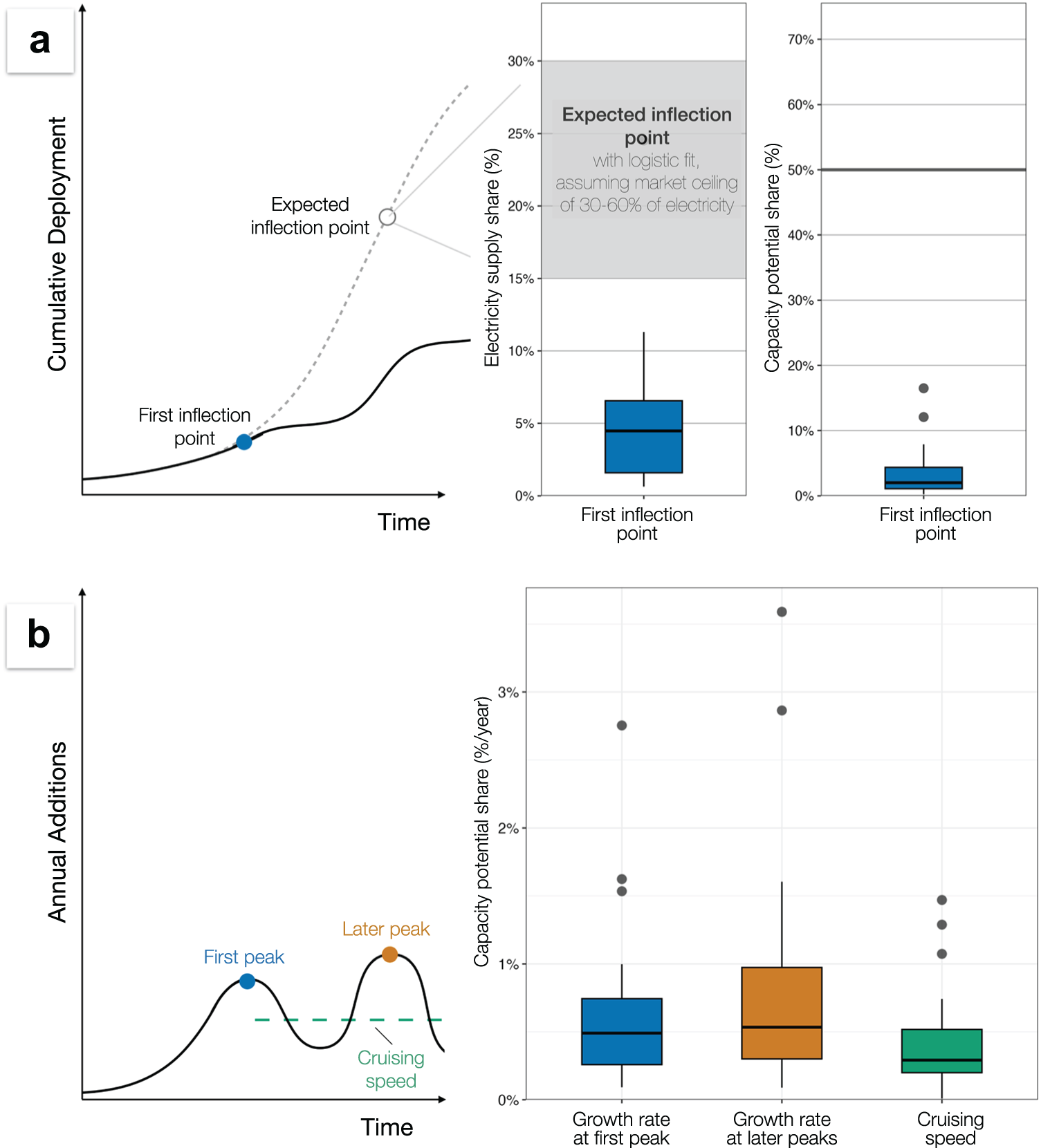
Consistent with our hypotheses, the growth of wind power in nearly all European countries experienced peaks after initial acceleration (Figure 2). The only exception is Czechia, where wind power has not taken off. Our algorithm also classifies Finland as still in the initial acceleration, despite a visible slowdown in 2016–2020. The first peaks (inflection points) occurred at relatively low levels of deployment, at 2% (IQR: 1–4%) of capacity potential, when wind generated 4% (IQR: 1.5–6%) of electricity (Figure 3a, Supplementary Table S3). This is early compared to standard S-curve expectations based on an assumption that wind can supply 30–60% of European electricity (European Commission, 2018; Fraile et al., Reference Fraile, Vandenberghe, Klonari, Ramirez, Pineda, Tardieu, Malvault and Komusanac2021), and therefore the inflection point of a standard logistic model should occur at around 15–30%.
Deployment levels at first peak (inflection point), growth rates at first and subsequent peaks, and the cruising speed.

Figure 3 Long description
The figure has two main panels. Panel A describes cumulative deployment and the timing of a first inflection point. On the left side of Panel A, a conceptual line chart plots cumulative deployment on the vertical axis against time on the horizontal axis. A black deployment curve rises slowly at first, reaches a blue point labeled “First inflection point,” then flattens before rising again later. A grey dashed S-shaped curve represents an expected cumulative deployment trajectory, with an open circle labeled “Expected inflection point” located higher and later than the observed first inflection point. Thin grey connector lines point from this expected inflection point to the adjacent data-based plots. To the right of the conceptual chart in Panel A are two vertical boxplots. The first boxplot has the vertical axis labeled “Electricity supply share (%)” and shows the electricity supply share at the first inflection point. The IQR box spans 1.5% to 6%, the median is 4%, and the upper whisker reaches 10%. A grey shaded band spans 15% to 30% and is labeled “Expected inflection point with logistic fit, assuming market ceiling of 30–60% of electricity.” The first-inflection-point distribution lies mostly below this expected range. The second boxplot has the vertical axis labeled “Capacity potential share (%)” and shows the first inflection point as a share of capacity potential. The IQR box spans 1% to 4%, the median is 2%, the upper whisker is below 10%, and two outliers are at 12% and 16%. A horizontal grey reference line is drawn at 50%. Panel B describes annual additions and growth-rate metrics. On the left side of Panel B, a conceptual line chart plots annual additions on the vertical axis against time on the horizontal axis. The black curve rises to a first peak marked by a blue point labeled “First peak,” declines, then rises again to a later peak marked by an orange point labeled “Later peak.” A green dashed horizontal line labeled “Cruising speed” runs across the later portion of the curve at a lower, steady level. This diagram defines the three quantities compared in the boxplots: growth rate at first peak, growth rate at later peaks, and cruising speed. On the right side of Panel B is a grouped boxplot with the vertical axis labeled “Capacity potential share (%/year).” The three boxplots correspond to “Growth rate at first peak,” “Growth rate at later peaks,” and “Cruising speed.” The first-peak boxplot is blue and has a median of 0.49% per year, with the IQR box spanning 0.26% to 0.74% per year. The later-peak boxplot is orange and has a median of 0.46% per year, with the IQR box spanning 0.28% to 0.97% per year. The cruising-speed boxplot is green and lower overall, with a median of 0.29% per year and the IQR box spanning 0.20% to 0.52% per year. Overall, the figure shows that peak growth rates at the first pulse and later pulses are similar, while cruising speed is lower than the peak rates.
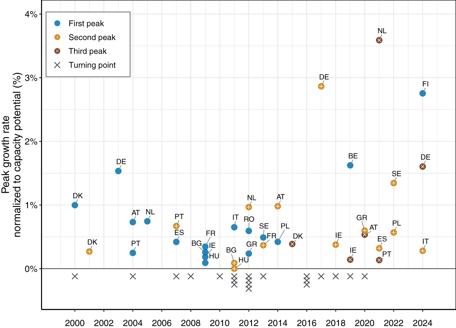
In line with our expectations, the range of peak growth rates at the first pulse (median 0.49% of capacity potential per year, IQR: 0.26–0.74) was similar to subsequent pulses (0.46%, IQR: 0.28–0.97) (Figure 3b). The median rate for secondary and tertiary peaks also remained almost the same before and after 2020 despite an outlier, the Netherlands (Figure 4). Within countries, deployment after the first inflection point typically continued at a cruising speed about one-quarter below the initial peak under both normalizations, with median cruising-to-first-peak ratios of 0.78 for capacity potential and 0.77 for electricity share (IQR: 0.34–1.15 and 0.59–1.66, respectively). Across countries, the cruising speed had a median of 0.29% of capacity potential per year (IQR: 0.20–0.52) and 0.72 percentage points (p.p.) of electricity share per year (IQR: 0.49–1.10) (Figure 3b).
Timing of peaks and turning points in individual countries.

Figure 4 Long description
The figure is a scatter plot showing the timing and peak rate of growth pulses across European countries. The horizontal axis shows years from 2000 to 2024. The vertical axis shows peak growth rate normalized to capacity potential, in percent, ranging from 0% to 4%. Each plotted point is labeled with a two-letter country code. Blue circles indicate first peaks, yellow circles indicate second peaks, brown circles indicate third peaks, and grey crosses indicate turning points. First peaks are distributed mainly between 2000 and 2014. Among first peaks occurring by 2014, Germany has the highest rate, at 1.53% in 2003, followed by Denmark, at 1.00% in 2000. One first peak occurs after 2014: Belgium at 1.62% in 2019 and Finland has not yet peaked by 2024. All other first peaks are below 1%. Second peaks span 2001 to 2024. The highest is Germany at 2.86% in 2017. Sweden has a second peak of 1.35% in 2022. Austria and the Netherlands have second peaks of 0.98% in 2014 and 0.97% in 2012, respectively. All remaining second peaks are below 0.7%. Third peaks occur in six countries between 2015 and 2024. The highest is the Netherlands at 3.59% in 2021, followed by Germany at 1.60% in 2024. The other third peaks are Austria at 0.53% in 2020, Denmark at 0.39% in 2015, Ireland at 0.14% in 2019, and Portugal at 0.13% in 2021. Grey crosses marking turning points extend from 2000 to 2020, with multiple turning points occurring in some years.
4.2. Early slowdown and pre-2021 reacceleration are induced by policy shifts
What drives these turning points and growth pulses? Turning points show some concentration around 2011–2012 (Figure 4), coinciding with two EU-wide developments documented by Pavlenko et al. (Reference Pavlenko, Jewell, Suzuki and Cherp2025): the implementation of the first Renewable Energy Directive (European Parliament and Council of the European Union, 2009), which set binding 2020 targets for all member states and prompted a wave of national support measures; and the prolonged eurozone debt crisis, which then forced austerity-driven rollbacks of renewable support across multiple member states. However, even this concentration is not statistically significant when accounting for the increasing number of countries in the sample (Monte Carlo p = 0.186, tested against a simulated null model accounting for the number of countries observed each year. The 37 peaks are even more evenly distributed over 25 years (Monte Carlo p = 0.649); thus, beyond this cluster, the timing of both peaks and turning points is asynchronous across countries. These observations, together with the  $ \sim $10-year pulse duration – much shorter than typical technology diffusion timescales (Iyer et al., Reference Iyer, Hultman, Eom, McJeon, Patel and Clarke2015) – point to national-level mechanisms, potentially political in nature, mediating these broader European drivers. A closer look at policy shifts confirms this connection.
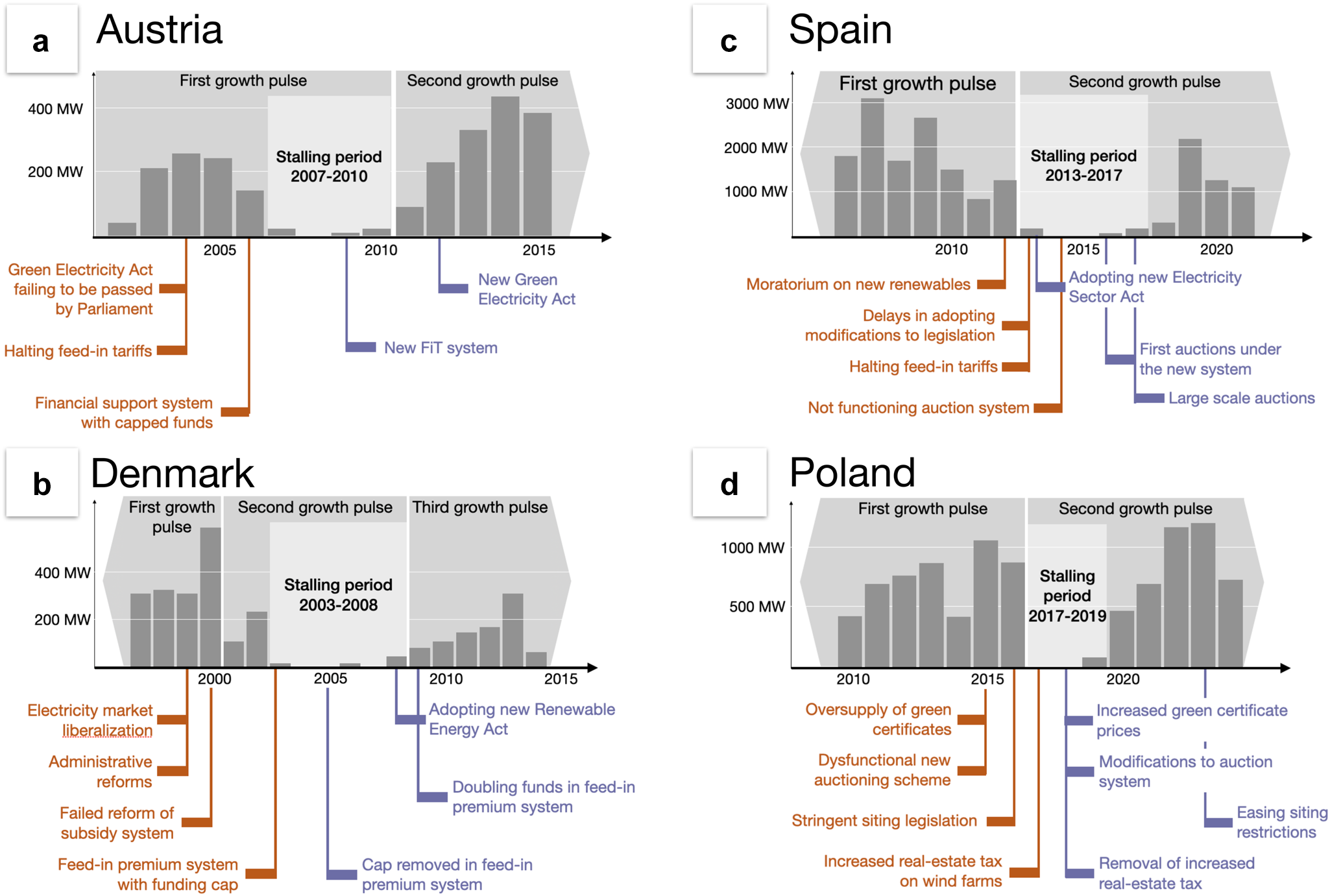
The first deviation from the standard S-curve – a relatively early slowdown after initial acceleration – has in every case coincided with cuts, moratoriums, or weakening of support (unless otherwise noted, policy shifts are sourced from CEER reports 2004–2025, see Section 3). In Spain, the moratorium and the retroactive abolition and restructuring of feed-in support ended initial acceleration, stalling deployment for 5 years (2013–2017). In Austria, the 2004 halt of FiT subsidies and subsequent regulatory uncertainty produced a four-year standstill. Denmark experienced a deployment collapse from 2003 to 2008 after electricity market liberalization and the failed attempt to replace FiTs with tradable green certificates. In Poland, three concurrent policy shocks from 2015–2017 – a dysfunctional auction system, the ‘10 H rule’ that excluded over 99% of land from wind development, and a tax increase on wind farms – stifled growth for several years (Supplementary Note S2, Section B). The same pattern extends to Italy (end of Green Certificate system in 2012), Greece (retroactive tariff cuts of  $ \sim $25% in 2012–2014), Bulgaria (FiTs for onshore wind were phased out by 2014), Hungary (a regulatory freeze through multiple mechanisms [Antal, Reference Antal2019; Szabo et al., Reference Szabo, Weiner, Deák, Knodt and Kemmerzell2021]), Sweden (certificate price collapse from 2018 [Windpower Monthly, 2019]), Romania (deferral of green-certificate revenue in 2013, effectively halving wind-farm income [Atănăsoae et al., Reference Atănăsoae, Pentiuc, Bobric and Hopulele2016]), Germany (the 2004 EEG revision that reduced tariffs while LCOE did not decline [Nacke et al., Reference Nacke, Jewell, Cherp and Bhowmik2026]), and Finland, where the 2011 FiT was closed to new applicants in 2017 (Renewables Finland, 2024). In each case, the policy disruption precedes or coincides with the inflection point (Supplementary Note S2, Section A and Figure 5). Conversely, countries whose trajectories did not experience drastic deceleration – Belgium, France, and Ireland – did not experience comparable policy disruptions during their main deployment periods (Supplementary Note S2, Section A).
Policy changes, growth pulses, and slowdown episodes in selected countries.

Figure 5 Long description
The figure has four panels showing annual onshore wind capacity additions and related policy events for Austria, Denmark, Spain, and Poland. Each panel contains a grey bar chart of annual capacity additions in megawatts, with years on the horizontal axis. Light grey shaded regions across the bar charts label periods of growth pulses and stalling periods. Policy events are annotated below the charts with vertical connector lines: orange annotations mark policy events associated with slowdowns or barriers, and purple annotations mark policy events associated with renewed support or recovery. Panel A shows Austria. The first growth pulse ends in 2010 and includes a stalling period between 2007 and 2010. Annual additions fell from 143 MW in 2006 to 23 MW in 2007 and remained below 23 MW per year through 2010. Orange annotations identify policy changes associated with this slowdown: the failure of amendments to the Green Electricity Act to pass Parliament and the halting of feed-in tariffs in 2004, followed by the introduction of a financial-support system with capped funds in 2006. A second growth pulse begins in 2010, with annual additions rising from 90 MW in 2011 to 436 MW in 2014 before declining again. Purple annotations identify subsequent supportive policy changes: the 2009 amendment introducing higher feed-in tariffs, which took effect in 2010, and the new Green Electricity Act adopted in 2011, and effective in 2012. Panel B shows Denmark. The first growth pulse ends in 2000, followed by a second pulse including a stalling period between 2003 and 2008. Annual additions fell from 233 MW in 2002 to 16 MW in 2003 and remained below 40 MW per year through 2008. Orange annotations identify policy changes associated with this slowdown: electricity-market liberalisation and administrative reforms in 1999, the failed reform of the subsidy system in 2000, and the introduction of a feed-in premium system with a funding cap in 2003. A third growth pulse begins in 2008, with annual additions rising from 82 MW in 2009 to 308 MW in 2013 before declining again. Purple annotations identify subsequent supportive policy changes: removal of the cap on the feed-in premium system in 2005, adoption of the new Renewable Energy Act in 2008, and doubling of financial support under the feed-in premium system in 2009. Panel C shows Spain. The first growth pulse ends in 2012, followed by a second pulse including a stalling period between 2013 and 2017. Annual additions fell from 1,260 MW in 2012 to 164 MW in 2013 and remained below 165 MW per year through 2017. Orange annotations identify policy changes associated with this slowdown: the moratorium on new renewable-energy support in 2012, delays in adopting legislative changes and the abolition of feed-in premiums in 2013, the 2013 Electricity Sector Act, and the introduction in 2014 of an auction-based support system that did not begin operating until 2017. Deployment subsequently recovered within the second pulse, with annual additions rising from 134 MW in 2017 to 281 MW in 2018 and 2,185 MW in 2019. Purple annotations identify policy changes that established the basis for this recovery: the 2013 Electricity Sector Act, the first national wind auction under the new system in 2016, and the substantially larger renewable-energy auctions in 2017. .Panel D shows Poland. The first growth pulse ends in 2016, followed by a second pulse including a stalling period between 2017 and 2019. Annual additions fell from 861 MW in 2016 to 12 MW in 2017 and remained below 72 MW per year through 2019. Orange annotations identify policy changes associated with this slowdown: the oversupply of green certificates and the dysfunctional auction system in the mid-2010s, stringent siting legislation adopted in 2016, and the increased real-estate tax on wind farms in 2017. Deployment recovered within the second pulse, with annual additions rising from 72 MW in 2019 to 460 MW in 2020 and 1,193 MW in 2023 before declining again. Purple annotations identify subsequent supportive policy changes: increased green-certificate prices, modification of the auction system and removal of the increased real-estate tax in 2018, followed by an easing of siting restrictions in 2023.
Secondary acceleration, which occurred in most countries, has led to pulses that can be divided into two approximately equal groups: those with peaks before and after 2021. The year 2021 was a watershed year for renewable energy policies as it marked a drastic increase in electricity prices, followed in 2022 by the outbreak of the Russia–Ukraine war that resulted in even higher prices and triggered a flurry of political activity in the energy sector (Pavlenko, Reference Pavlenko, Etkind and Morin2026). The pre-2021 pulses closely followed the introduction of new supportive policies. In Denmark, the 2008 Renewable Energy Act replaced the earlier premium-with-cap system with a 20-year feed-in premium, roughly doubling support and triggering a secondary pulse starting in 2008 and peaking in 2015 (IEA, 2008, 2013; Klima- Energi- og Forsyningsministeriet, 2008). In Austria, a pulse peaking in 2014 was driven by the 2009 ÖSG-Novelle, which reinstated financial support for onshore wind, and the 2012 Green Electricity Act, which tripled the funding envelope and earmarked support specifically for wind. Greece’s reacceleration in the mid-2010s was triggered by the 2016 renewable energy law. Poland’s reacceleration began after the June 2018 amendment unblocked the auction system, and the real-estate-tax increase was revoked. In Spain, the first national wind auction in 2016, followed by substantially larger renewable-energy auctions in 2017 launched a second pulse, which was later reinforced by high electricity prices, peaking in 2021 (see next section and Supplementary Note S2, Section B).
4.3. Starting from 2021, trajectories are affected by price dynamics, feature higher policy ambitions, but retain similar growth rates
Post-2020 trajectories suggest somewhat different policy-technology dynamics. To begin with, in some countries, deployment surged even after direct support policies had been removed. In Finland, the largest annual additions came in 2022–2024 despite the end of FiT support in 2017, driven by Power Purchase Agreements and other market mechanisms (Renewables Finland, 2024). In Sweden, certificate prices collapsed toward zero from 201 (Windpower Monthly, 2019), yet annual additions peaked in 2022 under de facto subsidy-free conditions. There has also been no obvious policy change leading to post-2020 surges in Austria, the Netherlands, Italy, and Portugal. In Spain and Poland, post-2020 pulses resulted from policy changes in 2017 and 2018, respectively (Supplementary Note S2, Section B). Only Germany’s recent acceleration has an obvious link with its post-2020 legislation (German Federal Government, 2023).
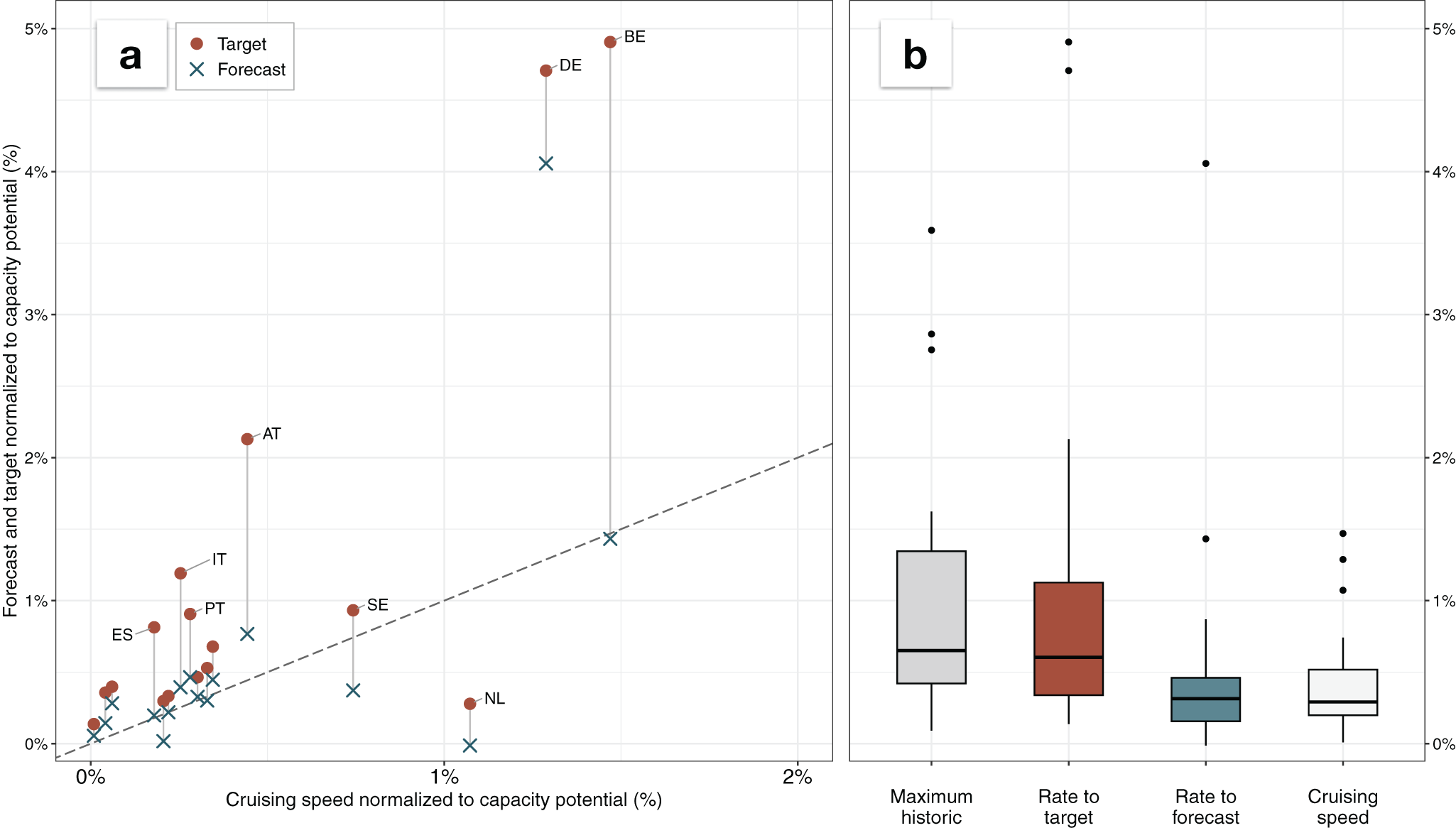
The recently adopted NECPs (European Commission, 2025), which set growth targets to 2030, provide a unique window into the role of policies in a period when technologies require fewer subsidies due to higher electricity prices and lower costs. These national targets and the overall European targets were often portrayed as ambitious, as they aimed to double the installed capacity (Pavlenko & Cherp, Reference Pavlenko and Cherp2026; Vinichenko et al., Reference Vinichenko, Jewell, Jacobsson and Cherp2023). Yet, interestingly, the target rates are close to the historical peak speeds (Figure 6), even though they were set under grid parity and heightened energy security concerns. Strikingly, however, forecasts (IEA, 2025b; WindEurope, 2026) are much closer to the cruising speed than the set targets (Figure 6 and Supplementary Figure S2). Germany remains a clear outlier on both targets and forecasts, consistent with its recent unprecedented policy effort granting overriding public interest status to wind and dedicating 2% of land area for wind development (Federal Ministry for Economic Affairs and Energy, 2022). Overall, the post-2020 targets and the prospects for their implementation show how policy ambitions increase under favorable market conditions coupled with energy security pressures. Even the increased ambitions do not exceed historical peak rates. At the same time, these increasing ambitions do not seem to lead to acceleration beyond cruising speed, signaling fundamental constraints to the latter.
Onshore wind growth rates implied by NECP targets and latest forecasts compared to cruising speed and maximum historical growth rates.

Figure 6 Long description
The figure has two panels comparing onshore wind deployment rates normalized to capacity potential. Panel A is a scatter plot comparing cruising speed with forecast and target rates, both normalized to capacity potential. The horizontal axis shows cruising speed, ranging from 0% to 2%, and the vertical axis shows forecast and target rates, ranging from 0% to 5%. Brown circles mark target rates and blue crosses mark forecast rates. A grey dashed diagonal line shows where forecast or target rates equal historical cruising speed. Points above the line are higher than cruising speed, and points below the line are lower. Forecast points are generally lower than the corresponding target points, often very close to the diagonal line indicating historic cruising speed. Most country values cluster in the lower-left corner, with cruising speeds below 0.5% of capacity potential and forecast or target rates below 1%. Spain, Italy, Portugal, and Austria have targets above their cruising speeds, while their forecasts remain close to cruising speed. Sweden’s target is close to cruising speed, but its forecast is lower. The Netherlands has both target and forecast values well below cruising speed. Germany and Belgium have the highest target rates, far above historical cruising speed; Belgium’s forecast is close to cruising speed, while Germany’s forecast is slightly below its target. Panel B contains four boxplots with the vertical axis again expressed as percent of capacity potential. The boxes, from left to right, show maximum historic rate, rate to target, rate to forecast, and cruising speed. The maximum historic boxplot has a median around 0.6%, with most values below about 1.5% and several high outliers near 2.7%, 2.9%, and 3.5%. The rate-to-target boxplot has a similar median, around 0.5% to 0.6%, but a wider spread and the highest outliers, reaching close to 5%. The rate-to-forecast boxplot is lower overall, with a median around 0.3%, most values below 0.5%, and outliers around 1.4% and 4%. The cruising-speed boxplot is also low, with a median around 0.3%, most values below 0.6%, and several outliers around 1.1% to 1.5%. Overall, the visual comparison shows that some target rates are far above countries’ historical cruising speeds, while most forecast rates are closer to the lower historical deployment-rate range.
5. Discussion and conclusions
Our analysis shows that the growth trajectories of onshore wind power in Europe systematically deviate from the expectations of standard S-curve diffusion theory. The initial acceleration is typically interrupted much earlier than expected – already when wind reaches about 2% (IQR: 1–4%) of its capacity potential – and this first inflection point closely follows the withdrawal, weakening, or destabilization of supporting policies. Yet the first turning point is not the start of a permanent slowdown as implied by monotonic feedback mechanisms. Instead, growth is shaped by the alternating dynamics of policy support. In most countries, growth reaccelerates through secondary and sometimes tertiary growth pulses, before 2021 led by policy changes and afterward reinforced by market dynamics.
Strikingly, the peak growth rate at successive pulses closely matches the rate at the first peak. This suggests that deployment speed is bounded by persistent constraints – most likely the fiscal space available for support instruments, permitting throughput, and the limits of social acceptance – rather than by steadily declining technology costs. Each new policy reform can restart growth, but it encounters a similar set of constraints, resulting in similar peak rates. The average rate of additions after the first inflection point – the ‘cruising speed’ (Jakhmola et al., Reference Jakhmola, Jewell, Vinichenko and Cherp2026b) – is about one-quarter below the first peak rate, reflecting not the weakening of individual pulses but the averaging of reacceleration phases with inter-pulse slowdowns when policy support falters.
From 2021, we observe a new dynamic. Lower technology costs and high electricity prices have enabled deployment to surge in some countries even after support instruments were withdrawn. In parallel, the recently adopted NECP targets, often portrayed as ambitious, in fact call for growth rates close to historically achieved peaks. Yet, even these targets are not expected to be met, with forecasts converging on the historical cruising speeds rather than peak rates, which underscores the persistence of constraints not easily addressed by political rhetoric or even by improved markets. The failure to achieve targets may also be connected to the fact that, somewhat paradoxically, the overall level of financial support to renewables declined from 2021 even as targets increased (Pavlenko & Cherp, Reference Pavlenko and Cherp2026). Germany stands out as the only country whose targets and forecasts substantially exceed its historical growth rates, consistent with its unprecedented policy effort to remove institutional barriers rather than merely increase financial incentives (Nacke et al., Reference Nacke, Jewell, Cherp and Bhowmik2026).
Our study advances the methodology for analyzing and projecting growth trajectories. Mainstream modeling of technology growth based on one-inflection S-curves assumes acceleration can be expected on the rising portion while slowdown follows the inflection point. The methods used to investigate trajectories are structured accordingly, centered on locating the inflection point, predicting the ceiling, and anticipating the duration of the S-curve (Baumgärtner et al., Reference Baumgärtner, Way, Ives and Farmer2024; Grubb et al., Reference Grubb, Drummond, Ives, Farmer and Kelkar2021; Way et al., Reference Way, Ives, Mealy and Farmer2022; Zielonka et al., Reference Zielonka, Wen and Trutnevyte2023). We develop a different approach that identifies segments of growth trajectories with distinct patterns and measures growth at multiple peaks as well as the cruising speed. This reveals dynamics of policy-driven technologies that single-model fitting obscures: turning points, growth pulses, and stagnation episodes. Our estimate of cruising speed at 0.72 p.p. of electricity supply per year (median; IQR: 0.49–1.10 p.p. per year) is broadly consistent with the maximum growth rate G estimated by Cherp et al. (Reference Cherp, Vinichenko, Tosun, Gordon and Jewell2021), but our analysis additionally provides evidence that the average growth speed is generally neither increasing nor decreasing after the first inflection point. The multi-segment approach also enables systematic mapping of turning points against documented policy shifts, providing a more granular evidence base for causal analysis than aggregate cross-country regressions.
Our analysis advances understanding of phases of policy-driven technology transitions. Prior literature has shown that distinct growth phases are shaped by both technological and socio-political factors (Cherp et al., Reference Cherp, Vinichenko, Tosun, Gordon and Jewell2021; Jewell et al., Reference Jewell, Cherp, Geels, Suzuki, Nacke, Tosun, Bhowmik, Kazlou, Jakhmola and Vinichenko2026), but has not examined whether technology diffusion and policy change are synchronized in timing and aligned in direction. We find that, at least for onshore wind power in Europe, they are not: policy cycles often diverge from diffusion trends in both timing and direction, producing multiple turning points rather than a linear sequence of phases.
Our findings also inform how policy-driven acceleration is conceptualized. Jewell et al. (Reference Jewell, Cherp, Geels, Suzuki, Nacke, Tosun, Bhowmik, Kazlou, Jakhmola and Vinichenko2026) define acceleration in the steady growth phase as either a higher linear growth rate or the avoidance of slowdown (see also Sovacool et al., Reference Sovacool, Geels, Andersen, Grubb, Jordan, Kern, Kivimaa, Lockwood, Markard, Meadowcroft, Meckling, Moore, Raven, Rogge, Rosenbloom, Schmidt, Schot, Sharp, Stephenson, Vormedal and Yang2025). We support this interpretation and propose a real-world benchmark for ‘faster’ growth: the speed observed at the first peak (inflection point). While later peaks in individual countries may occasionally exceed this level, the range of peak growth rates across countries remains stable. We further examine whether this benchmark holds once technologies become economically competitive and policies shift away from direct financial support. In this context, growth peaks remain similarly prevalent and average growth rates persist at comparable levels despite more ambitious targets. Exceeding historical benchmarks appears rare and typically requires dedicated policy interventions, as illustrated by Germany (Nacke et al., Reference Nacke, Jewell, Cherp and Bhowmik2026).
Our analysis is specific to onshore wind in the EU: a capital-intensive, relatively decentralized but complex technology that requires local customization (Binz & Truffer, Reference Binz and Truffer2017) where deployment depends heavily on national support. Whether our findings about growth trajectories generalize to other types of technologies and contexts should be investigated in future research that could extend our framework to other policy-driven technologies – solar PV, offshore wind, heat pumps – and to regions where institutional contexts and policy capacities differ from Europe. Jakhmola et al. (Reference Jakhmola, Jewell, Vinichenko and Cherp2026b) provide a promising example of such a study. Onshore wind in Europe is also a technology which is both beyond its formative phase (i.e., a mature technology in this region) and still far away from saturation. For technologies that are still locally in the formative or slowdown phases, the effect of policy interventions may differ (Jewell et al., Reference Jewell, Cherp, Geels, Suzuki, Nacke, Tosun, Bhowmik, Kazlou, Jakhmola and Vinichenko2026; Markard et al., Reference Markard, Geels and Raven2020). Further research should also investigate the relative contributions of non-policy factors, including macroeconomic cycles, supply-chain bottlenecks, and shifts in social acceptance, to the presence, timing, and magnitude of growth pulses. In part, this could be done by comparing the trajectories of policy-driven technologies and those historically driven by market forces and innovation (Jakhmola et al., Reference Jakhmola, Jewell, Vinichenko and Cherp2026b).
Our policy analysis demonstrates a strong temporal association between policy shifts and growth turning points, but we do not claim that policy is the sole driver: macroeconomic conditions, supply-chain dynamics, and social acceptance also play a role. The 4-year minimum segment length may miss shorter policy effects, and the capacity-potential estimates used for normalization carry uncertainty about national conditions; these limitations could be addressed in future studies. In the future, it would be particularly valuable to investigate what specific policy designs and institutional reforms (permitting, grid planning, spatial allocation) can sustain deployment at peak rates rather than cruising speed, effectively raising the country-specific ceiling. Connecting the growth-pulse framework with the broader literature on socio-technical transitions and the political economy of energy policy could yield insights into the conditions under which reacceleration is possible – and what it would take to sustain the speeds required to meet 2030 climate targets.
Supplementary material
The supplementary material for this article can be found at https://doi.org/10.1017/sus.2026.10086.
Acknowledgements
The authors are grateful for the valuable discussions and feedback they have received on earlier drafts of this paper at their respective research institutions and from participants of the European Consortium for Political Research (ECPR) Joint Sessions 2024 workshop.
Author contributions
Conceptualization (M.V., V.V., J.J., A.P., A.C.), Data acquisition and curation (M.V., A.P.), Formal analysis (M.V., V.V., A.P.), Funding acquisition (J.J., A.C.), Investigation (M.V., A.P., A.C.), Methodology (M.V., V.V., J.J., A.P., A.C.), Project administration (M.V., J.J., A.C.), Resources and software (V.V.), Supervision (J.J., A.C.), Visualization (M.V., V.V., A.C.), Writing – original draft (M.V., V.V., J.J., A.P., A.C.), Writing – review and editing (M.V., V.V., J.J., A.P., A.C.).
Data availability statement
The research was based on publicly available data; no further data have been generated during this work.
Funding statement
The authors thank the following sources for financial support. M.V.: MISTRA Electrification research program funded by the Swedish foundation for strategic environmental research (MISTRA), and NEWSTEPS project funded by the Swedish Energy Agency; V.V.: MANIFEST project (no. 950408) funded by the European Commission's Horizon 2020 ERC Starting Grant; A.P.: MISTRA Electrification research program funded by the Swedish Foundation for Strategic Environmental Research (MISTRA); J.J.: MANIFEST project (no. 950408) funded by the European Commission's Horizon 2020 ERC Starting Grant, MISTRA Electrification research program funded by the Swedish Foundation for Strategic Environmental Research (MISTRA); and NEWSTEPS project funded by the Swedish Energy Agency. A.C.: MISTRA Electrification research program funded by the Swedish Foundation for Strategic Environmental Research (MISTRA), and NEWSTEPS project funded by the Swedish Energy Agency.
Competing interests
The authors declare no competing interests.


 Open access

