1. Introduction
Jets of fluid emerging from a circular tube are encountered in many applications. These include propulsion of large aircraft to microjets used for cooling in electronic circuits. The jet should be highly directional if used as a thruster and must spread maximally if used for mixing. Jets are also a source of noise and may need to be suitably controlled. In view of its importance, considerable research has been devoted towards understanding the evolution of jets. Problems of diverse nature such as noise generation, mixing and flame stability are intimately linked to jet instabilities and the formation of vortex rings, which are large-scale coherent structures in the flow field.
The strength of flow structures and their point of initiation can be externally controlled. A possibility is to actuate the nozzle on its exit plane, thus forcing the jet emanating into the ambient. Preliminary research shows that a forced jet displays large-scale effects in the development and characteristics of the flow field. The inflow perturbation at both large and small scales can augment entrainment, spreading and mixing.
An understanding of the instability mechanisms in free jets and the formation of coherent structures helps in the design of active control strategies that enhance the spreading of the jet. In the present study, the temporal characteristics of the background instability of a free jet have been used to define active control. These perturbations are classified as varicose (axisymmetric), flapping and dual-mode. Analysis suggests that the varicose mode is the most fundamental one in the shear layer instability of circular jets. It can be realized by applying a time periodic excitation to the entire nozzle at a particular forcing frequency and amplitude. This approach can be used to control the generation of vortex rings as well as the distance between consecutive vortex rings. Dual-mode perturbation is obtained by combining axisymmetric excitation with the helical mode, where pulsations appear by a rhythmic undulation or twisting of the jet. The frequency ratio of the two modes of perturbation plays a significant role in jet control.
Reynolds et al. (Reference Reynolds, Parekh, Juvet and Lee2003) experimentally studied the evolution of a circular jet using dual-mode excitation. They showed the formation of two distinct types of jets – bifurcating and blooming. These were accompanied by a spectacular increase in jet spreading. In a bifurcating jet, two branches on the bifurcating plane were clearly formed. For irrational values of the frequency ratio, Reynolds et al. (Reference Reynolds, Parekh, Juvet and Lee2003) suggested that the jet can be made to bloom, leading to ‘an amazing shower of vortex rings’. A few numerical studies in the literature discuss jet bifurcation. There is no computational study available on blooming of a forced jet. Direct numerical simulation (DNS) of a jet perturbed at its inflow plane has been carried out in the present work at a Reynolds number of 2000, which is based on the nozzle diameter,
 $D$
, and the maximum nozzle exit velocity,
 $U_{\mathit{inlet}}$
.
The paper is organized as follows. The literature on jet control is first reviewed. The numerical methodology is DNS, and it is described along with the simulation parameters. Validation, grid and domain independence studies are presented next. Results are described with the help of instantaneous snapshots as well as selected time-averaged three-dimensional flow fields for various controlling parameters. Conclusions form the final section.
2. Background literature
Jet control has attracted a great deal of attention over the past decade. Since large scales of fluid motion play a primary role in transport phenomena, selective manipulation of these structures is needed to achieve efficient control (Cantwell Reference Cantwell1981; Ho & Huerre Reference Ho and Huerre1984; Robinson Reference Robinson1991). Excitation can result in an amplification of instabilities in the mixing layer and increase the strength of the vortical structures (Crow & Champagne Reference Crow and Champagne1971; Moore Reference Moore1977; Hussain & Zaman Reference Hussain and Zaman1980). The potential core is also shortened because of the perturbation and is a sign of greater mixing (Lepicovsky, Ahuja & Burrin Reference Lepicovsky, Ahuja and Burrin1985).
2.1. Forced jets
Active control of flow along with momentum and scalar transport has been a central theme in the work of many authors (Moin & Bewley Reference Moin and Bewley1994; Gad-el-Hak Reference Gad-el-Hak1996; Kasagi Reference Kasagi1998). There are two ways to force the flow: mechanically, with an oscillating flap at the exit of the nozzle, and acoustically, with loudspeakers inside the nozzle. The present work aims at exciting a jet at its preferred mode frequency, with the expectation that large structures will form. For the design of such an inlet perturbation, three input parameters are required. These are the frequency of excitation, the excitation level and the mode of excitation. Prior research related to these approaches is presented below.
2.1.1. Frequency of excitation
The literature on forced jets shows the preferred mode frequency and the subharmonic frequency of the undisturbed jet to be important. The preferred mode frequency is the natural frequency associated with large-scale structures in a free jet. The growth of the subharmonic mode in a jet is related to alternate pairing of vortex rings. Interesting results have been obtained from subharmonic forcing both in numerical simulation (Patnaik, Sherman & Corcos Reference Patnaik, Sherman and Corcos1976; Riley & Metcalfe Reference Riley and Metcalfe1980) and in experimental studies (Zang, Ho & Monkewitz Reference Zang, Ho, Monkewitz and Kozlov1985; Hajj, Miksad & Powers Reference Hajj, Miksad and Powers1992). Theoretical studies on subharmonic forcing have been carried out by Kelly (Reference Kelly1967), Nikitopoulos & Liu (Reference Nikitopoulos and Liu1987) and Monkewitz (Reference Monkewitz1988).
The degree of jet spreading offered by a single-frequency plane wave excitation may not seem attractive enough for practical applications. However, when the preferred mode frequency becomes neutrally stable, its subharmonic, which amplifies rapidly, can be used to cause mixing and enhancement of momentum transport. An analysis presented by Kelly (Reference Kelly1967) showed that there exists a mechanism for the generation of a subharmonic for a tangent hyperbolic velocity profile with an inflexion point. It was shown later by Ho & Huang (Reference Ho and Huang1982) that the spreading rate of a mixing layer can be improved significantly by forcing near the subharmonic of the preferred frequency. Furthermore, when the shear layer is excited simultaneously by the fundamental and the subharmonic, a large augmentation of the subharmonic amplitude can occur. Some aspects of this question have been addressed by Cohen & Wygnanski (Reference Cohen and Wygnanski1987) and Ng & Bradley (Reference Ng and Bradley1988).
2.1.2. Excitation level
The excitation amplitude needs to be correctly chosen for proper control. Crow & Champagne (Reference Crow and Champagne1971) characterized the excitation level in terms of the turbulent intensity at the centreline of the jet as a function of the forcing amplitude. The plot shows a linear relationship for an excitation range of 0.1–1 %, beyond which it reaches saturation. If the excitation is low, no control is possible. If it is high, the entire power spectrum suffers nonlinear distortion. At an optimum excitation level, the power spectrum does not differ from the unforced spectrum except over a narrow band centred on the forcing frequency.
2.1.3. Modes of excitation
Long & Petersen (Reference Long and Petersen1990) performed excitation with helical waves for an axisymmetric jet. The shape of the jet cross-section was seen to change with the mode number,
 $m$
. It was elliptic for a combination of
 $m=+1$
and
 $m=-1$
, and square for a combination of
 $m=+2$
and
 $m=-2$
. Pashereit et al. (Reference Pashereit, Oster, Long, Fiedler and Wygnanski1992) showed the visualization of patterns arising from the secondary interaction of helical and axisymmetric modes. In an earlier study, azimuthal modulation was seen to control the cross-sectional shape of the isovelocity contours in the near field (Cohen & Wygnanski Reference Cohen and Wygnanski1987).
Acoustic forcing can also influence the pairing between fundamental and subharmonic vortices. A phase difference between the two frequencies affects the pairing. The relative phase of the two modes is a determining factor of the intramodal energy transfer (Monkewitz Reference Monkewitz1988). The possibility of coalescence of two vortices increases as the phase difference decreases. When the phase difference is
 ${\rm\pi}$
, no pairing occurs. Instead, a shedding interaction takes place. Petersen & Clough (Reference Petersen and Clough1992) observed improved resonant interaction in forcing the
 $3/2$
harmonic, the fundamental and the subharmonic rather than the last two alone. A three-mode interaction has been theoretically explained by Nikitopoulos & Liu (Reference Nikitopoulos and Liu1987) in a mixing layer as providing a weak direct effect and a strong indirect effect on the flow.
2.2. Active control
Here, the reference is to a methodology of affecting the flow evolution by introducing externally powered perturbations into the fluid medium.
Crow & Champagne (Reference Crow and Champagne1971) reported results related to jet control when a loudspeaker was devised for excitation. By superimposing several frequencies
 $f$
at the jet inlet, the maximum amplification of the initial perturbation was studied at the end of the potential core (
 $x/D=4$
, where
 $x$
is the streamwise direction). The maximum was seen at a Strouhal number of
 $\mathit{St}_{D}=fD/U_{\mathit{inlet}}=0.3$
. Within limits, this observation was found to be independent of the Reynolds number. Consequently, the particular frequency was denoted as the preferred mode as it showed the strongest response in the jet. It was further noticed that a natural unforced jet has a peak frequency right at this preferred mode which corresponds to the periodic passage of vortical structures at the end of the potential core. The authors further noticed increase in the spreading rate between 0 and
 $x/D=8$
. Crow & Champagne (Reference Crow and Champagne1971) and Ginevsky, Vlasov & Karavosov (Reference Ginevsky, Vlasov and Karavosov2004) have both shown that the dynamical character of the flow field strongly responds to the applied forcing frequency. This attribute can be used to achieve a jet of desired character, as active forcing at certain discrete frequencies may either promote or suppress the formation of vortical structures.
Corke & Kusek (Reference Corke and Kusek1993) introduced localized acoustic disturbances, which were produced by an array of miniature loudspeakers placed around the jet nozzle. They investigated the effect of forcing by axisymmetric and counter-rotating helical modes. Smith & Glezer (Reference Smith and Glezer1997) successfully applied miniature zero-mass-flux jet actuators for the control of a large-scale planar jet. The primary jet could be vectored either towards or away from the synthetic jet actuators by creating a low-pressure recirculation region.
Many experimental studies on jet control have focused on enhancement of the jet spreading rate (Lee & Reynolds Reference Lee and Reynolds1985a
,Reference Lee and Reynolds
b
; Corke & Kusek Reference Corke and Kusek1993; Longmire & Duong Reference Longmire and Duong1996; Suzuki, Kasagi & Suzuki Reference Suzuki, Kasagi and Suzuki1999, Reference Suzuki, Kasagi and Suzuki2004). Lee & Reynolds (Reference Lee and Reynolds1985a
,Reference Lee and Reynolds
b
) demonstrated a dramatic increase in the jet spreading by combining the axisymmetric disturbance with a helical one. Bifurcating jets display a substantial increase in the spreading rate along one particular plane (the bifurcating plane) while maintaining an unchanged or even reduced spreading rate along a perpendicular plane (the bisecting plane). The authors showed how simultaneous axisymmetric and orbital excitations can be used to increase the growth of the shear layer in the bifurcating plane. For the range of Reynolds numbers considered (
 $2800<\mathit{Re}_{D}<10\,000$
), the spreading of the jet was found to depend solely on the ratio between the axisymmetric frequency
 $(\,f_{a})$
and the helical (orbital) frequency
 $(\,f_{o})$
,
 $R_{f}=f_{a}/f_{o}$
. The ranges of Strouhal numbers used were
 $0.35<f_{a}D/U_{\mathit{inlet}}<0.75$
and
 $0.15<f_{o}D/U_{\mathit{inlet}}<0.35$
for axisymmetric and orbital excitations respectively. For
 $R_{f}=2$
, a bifurcating jet was obtained in which the primary vortex rings were expelled towards two opposite directions in the bifurcating plane. For
 $R_{f}=3$
, the jet spread into three branches (trifurcating jet). For non-integer values of
 $R_{f}$
in the interval
 $1.6<R_{f}<3.2$
, the jet branched in all directions and blooming jets were formed.
Suzuki et al. (Reference Suzuki, Kasagi and Suzuki1999, Reference Suzuki, Kasagi and Suzuki2004) experimentally studied a bifurcating jet resulting from small flap actuators placed on the sidewalls of the jet nozzle. Maximum spreading in the bifurcating plane was obtained for a Strouhal number based on the flapping frequency of
 $\mathit{St}_{f}=0.25$
. This value is approximately one-half of the preferred Strouhal number measured in a natural jet (
 $=0.52$
). The range of Reynolds numbers investigated was up to
 $\mathit{Re}_{D}<13\,000$
. The flapping amplitude was quite high, the streamwise velocity fluctuation being approximately 10 % of the average amplitude of a natural jet. Another experimental study of bifurcating jets at high Reynolds numbers was performed by Parekh, Leonard & Reynolds (Reference Parekh, Leonard and Reynolds1988) using four loudspeakers at the jet inlet. Using a combination of axisymmetric and flapping perturbations, they showed that bifurcating jets can still be generated at very high Reynolds numbers (
 $1.0\times 10^{4}<Re_{D}<1.0\times 10^{5}$
) with a forcing amplitude of 15 % of the inlet velocity profile.
There are very few numerical studies dealing with jet control. Urbin & Métais (Reference Urbin, Métais, Chollet, Voke and Kleiser1997) applied specific perturbations at the inlet of a spatially growing round jet. They performed large-eddy simulation with various inlet perturbations and could trigger axisymmetric, helical and alternate pairing modes. An impressive spreading of the jet along a preferential plane was observed, bearing strong similarity to bifurcating jets realized in experiments. With this excitation, the primary rings of the jet were seen to be alternately inclined with respect to their axis, creating a zigzag arrangement and localized pairings. Danaila & Boersma (Reference Danaila and Boersma1998, Reference Danaila and Boersma2000) revisited the work of Urbin & Métais (Reference Urbin, Métais, Chollet, Voke and Kleiser1997) by using DNS at a low Reynolds number (
 $\mathit{Re}_{D}=1500$
). They recovered the original trends with flapping excitation. Moreover, Danaila & Boersma (Reference Danaila and Boersma2000) created jet bifurcation from a combination of axisymmetric and flapping excitation. Although both flapping and bifurcating excitations caused a drastic increase of the spreading rate in the bifurcating plane, the statistical and topological features of the two jets were found to be quite distinct. Furthermore, bifurcating excitation induced the largest spreading rate only in the bifurcating plane. It is to be mentioned that Urbin & Métais (Reference Urbin, Métais, Chollet, Voke and Kleiser1997) used a much lower excitation amplitude (5 %) compared with the 15 % of Danaila & Boersma (Reference Danaila and Boersma2000).
da Silva & and Métais (Reference da Silva and Métais2002) performed direct and large-eddy simulations to analyse vortex dynamics and the statistics of bifurcating jets in the Reynolds number range of
 $1.5\times 10^{3}{-}5.0\times 10^{4}$
. Flapping excitation was imposed at both the preferred mode and subharmonic frequencies. Results of combined varicose and flapping excitation were also documented. Although it was possible to have bifurcation at low Reynolds numbers using flapping excitation, it became difficult to achieve bifurcation at high Reynolds numbers. Fragmentation of the larger vortices due to transition to turbulence led to loss of flow control. da Silva & and Métais (Reference da Silva and Métais2002) also reported that varicose excitation at the preferred mode combined with the flapping excitation at the subharmonic frequency causes the jet to have large spreading rates, while being insensitive to the Reynolds number.
The authors of the present work have previously studied the characteristics of a forced circular jet subjected to flapping excitation and observed bifurcation (Y) as well as trifurcation (
 ${\rm\Psi}$
) patterns for certain forcing parameters (Gohil, Saha & Muralidhar Reference Gohil, Saha and Muralidhar2010). Direct numerical simulation of spatially developing circular jets was reported by the authors at a moderate Reynolds number of 1030 (Gohil, Saha & Muralidhar Reference Gohil, Saha and Muralidhar2011). Sinuous and varicose instabilities in a free circular jet were demonstrated for a Reynolds number range of 500–2000 (Gohil, Saha & Muralidhar Reference Gohil, Saha and Muralidhar2012). Later, Gohil, Saha & Muralidhar (Reference Gohil, Saha and Muralidhar2013, Reference Gohil, Saha and Muralidhar2014) investigated the influence of axial perturbation on jet evolution and flow structures using a computational approach. In these studies, instantaneous as well as time-averaged flow fields were presented. Apart from the experimental work of Reynolds et al. (Reference Reynolds, Parekh, Juvet and Lee2003), the survey of the literature reveals analysis of forced jets subjected to only a single perturbation. Dual-mode forcing and the possibility of jet blooming have not been numerically studied, forming the motivation of the present study. In the present work, the possibility of formation of multiple branched jets observed by Reynolds et al. (Reference Reynolds, Parekh, Juvet and Lee2003) is examined via DNS. The relation between the forcing parameters and the number of branches as well as the time-averaged jet spreading and entrainment are studied.
3. Numerical methodology
Numerical simulation of a perturbed jet is performed by solving the unsteady three-dimensional incompressible Navier–Stokes equations, written as
 $$\begin{eqnarray}\displaystyle & \displaystyle \frac{\partial u_{i}}{\partial x_{i}}=0, & \displaystyle\end{eqnarray}$$
 $$\begin{eqnarray}\displaystyle & \displaystyle \frac{\partial u_{i}}{\partial t}+\frac{\partial }{\partial x_{j}}(u_{i}u_{j})=-\frac{\partial p}{\partial x_{i}}+\frac{1}{\mathit{Re}}\frac{\partial ^{2}u_{i}}{\partial x_{j}^{2}}. & \displaystyle\end{eqnarray}$$
Equations (3.1) and (3.2) are non-dimensionalized using the nozzle diameter,
 $D$
, and the maximum nozzle exit velocity,
 $U_{\mathit{inlet}}$
, while time and pressure,
 $p$
, are non-dimensionalized using
 $D/U_{\mathit{inlet}}$
and
 ${\it\rho}U_{\mathit{inlet}}^{2}$
respectively.
The numerical algorithm that solves (3.1) and (3.2) is based on the marker and cell (MAC) formulation proposed by Harlow & Welch (Reference Harlow and Welch1966). Temporally, a second-order Adams–Bashforth scheme is employed for the convective terms while the diffusion terms are discretized using a Crank–Nicolson scheme. With this approach, the viscous stability constraint is eliminated and the flexibility in the choice of the time step is increased. The pressure-correction Poisson equation is solved using a Gauss–Seidel successive over-relaxation (GSSOR) approach. The equations are discretized on a staggered grid. The convective terms are discretized spatially using a weighted averaged fourth-order central difference scheme and a fifth-order upwind-biased scheme and the diffusion terms are discretized using a fourth-order central difference scheme. Unlike upwind schemes, a central difference discretization is found to be free from artificial/numerical dissipation. However, because of aliasing error, central difference schemes suffer from the difficulty of divergence in the iterative solution unless very fine grids that satisfy the stability constraint are utilized. As an alternative, the convective terms are discretized spatially using a weighted averaged fourth-order central difference scheme combined with a fifth-order upwind-biased scheme (Rai & Moin Reference Rai and Moin1991). For the resulting improvement in accuracy, upwind-biased difference schemes require a much smaller stencil compared with a fully upwind method. The use of fine grids in the present study helps in retaining information in the high-frequency part of the spectrum of the physical flow field that would otherwise be damped by upwinding. The percentage contribution of the fifth-order upwind-biased scheme is limited to 10–15 % relative to the fourth-order central difference formula. The discretization of diffusion terms is carried out using a fourth-order central difference scheme. For non-uniform meshes, the coefficients in the difference formulae are evaluated numerically in the computer code using the Fornberg algorithm (Fornberg Reference Fornberg1988). Code parallelization is carried out with the help of message passing interface (MPI) libraries. The detailed method of solution is explained in the prior work of the authors (Gohil et al. Reference Gohil, Saha and Muralidhar2010, Reference Gohil, Saha and Muralidhar2011, Reference Gohil, Saha and Muralidhar2012).
On the inlet boundary, the time-dependent velocity profile is prescribed as
 $$\begin{eqnarray}\left.\begin{array}{@{}c@{}}u_{x}^{\mathit{inlet}}(r,t)=u_{x}^{\mathit{profile}}(r)+u_{x}^{\mathit{noise}}(r,t)+u_{x}^{\mathit{forced}}(r,t),\\ u_{y}^{\mathit{inlet}}(r,t)=u_{y}^{\mathit{noise}}(r,t),\\ u_{z}^{\mathit{inlet}}(r,t)=u_{z}^{\mathit{noise}}(r,t).\end{array}\right\}\end{eqnarray}$$
Here,
 $u_{x}^{\mathit{inlet}}(r,t)$
is the instantaneous inlet velocity (streamwise) and
 $r=\sqrt{y^{2}+z^{2}}$
. The expression for
 $u_{x}^{\mathit{profile}}(r)$
is given by (3.4) below, while
 $\boldsymbol{u}_{i}^{\mathit{noise}}(r,t)$
(
 $i=x,y,z$
) and
 $u_{x}^{\mathit{forced}}(r,t)$
are components of random and large-scale perturbations respectively. The subscript ‘
 $i$
’ can take any value among the
 $x$
,
 $y$
and
 $z$
coordinates depending on the velocity component.
The time-averaged streamwise velocity variation given by Michalke & Hermann (Reference Michalke and Hermann1982) is used at the inflow plane. It is known to be a good approximation of the measured velocity profiles in round jets at a location close to the nozzle exit. The modelled streamwise velocity is given as
 $$\begin{eqnarray}u_{x}^{\mathit{profile}}(r)=\frac{U_{\mathit{inlet}}}{2}\left\{1+\tanh \left[\frac{R-r}{2{\it\theta}_{m}}\right]\right\}.\end{eqnarray}$$
Here,
 $R=D/2$
and
 ${\it\theta}_{m}$
is the momentum thickness of the shear layer at the nozzle exit. In most experimental apparatus, background disturbances in the form of non-uniformity in the inlet velocity profile, surface roughness and inherent vibrations prevail. The jet characteristics are sensitive to these disturbances. In the present study, a random Gaussian perturbation,
 $\boldsymbol{u}_{i}^{\mathit{noise}}(r,t)$
, with root mean square value varying between 0 % and 5 % of the space-averaged velocity is added to the three components of the velocity vector at the inlet. A non-reflective outflow condition is used at the exit plane of the physical domain (Orlanski Reference Orlanski1976). The confining surfaces transverse to the jet are modelled as periodic boundaries. The ratio of the jet radius to the initial momentum thickness of the boundary layer is varied over 10–90. With this choice, both instabilities, helical and axisymmetric, are expected to grow in the downstream direction (Cohen & Wygnanski Reference Cohen and Wygnanski1987).
In dual-mode excitation, forcing of the jet is obtained by a combination of an axisymmetric excitation at the preferred mode frequency and helical excitation (
 $m=1$
). The helical mode frequency is fixed by the excitation frequency ratio,
 $R_{f}=\mathit{St}_{D}/\mathit{St}_{H}$
, where
 $\mathit{St}_{D}$
and
 $\mathit{St}_{H}$
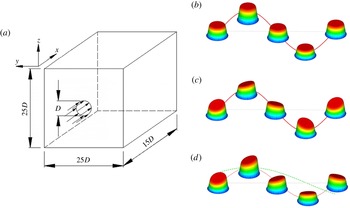
are the axisymmetric and helical Strouhal numbers respectively. The streamwise velocity profiles at the nozzle exit for varicose, helical and dual-mode excitation are shown in figure 1.
(a) Computational domain and (b–d) three-dimensional representations of the streamwise velocity profiles at the nozzle exit for various excitations: (b) varicose excitation, (c) helical excitation and (d) dual-mode excitation. It should be noted that dual-mode excitation is characterized by two frequencies and hence a frequency ratio
 $R_{f}$
.

The expression for the time- and space-dependent excitation is now given as
 $$\begin{eqnarray}\displaystyle u_{x}^{\mathit{forced}}(r,t) & = & \displaystyle \left\{A_{n}u_{x}^{\mathit{profile}}(r)\sin \left(2{\rm\pi}\mathit{St}_{D}\frac{U_{\mathit{inlet}}}{D}t\right)\right\}\nonumber\\ \displaystyle & & \displaystyle +\left\{A_{h}u_{x}^{\mathit{profile}}(r)\sin \left(2{\rm\pi}\mathit{St}_{H}\frac{U_{\mathit{inlet}}}{D}t-{\it\theta}_{c}\right)\left(\frac{2r}{D}\right)\right\}.\end{eqnarray}$$
The amplitudes of the imposed varicose and helical excitations are
 $A_{n}$
and
 $A_{h}$
, and
 ${\it\theta}_{c}$
is the azimuthal direction in cylindrical coordinates. In the present study, equal amplitudes have been used for axisymmetric and helical perturbation (
 $A_{n}=A_{h}$
). The excitations given by (3.5) are applied to the streamwise velocity component, while for the transverse velocity components, they are set to zero.
The
 $Q$
criterion, which deals with the second invariant of the velocity gradient tensor (Hunt, Wray & Moin Reference Hunt, Wray and Moin1988), is used in the present work to extract the vortical structures from the simulation data. The
 $Q$
function is given as
 $$\begin{eqnarray}Q=1/2({\it\Omega}_{ij}{\it\Omega}_{ij}-\unicode[STIX]{x1D61A}_{ij}\unicode[STIX]{x1D61A}_{ij}).\end{eqnarray}$$
Further,
 $$\begin{eqnarray}{\it\Omega}_{ij}=(\partial u_{i}/\partial x_{j}-\partial u_{j}/\partial x_{i})/2\quad \text{and}\quad \unicode[STIX]{x1D61A}_{ij}=(\partial u_{i}/\partial x_{j}+\partial u_{j}/\partial x_{i})/2\end{eqnarray}$$
are the antisymmetric and symmetric parts of the velocity gradient tensor
 $(\partial u_{i}/\partial x_{j})$
. Positive
 $Q$
isosurfaces isolate areas where the strength of rotation overcomes strain, thus making those surfaces eligible as vortex envelopes. Since the vorticity should increase towards the centre of the vortex, the function
 $Q$
can be expected to remain positive in the vortex core.
3.1. Simulation details
One of the important controlling parameters in dual-mode perturbation is the excitation frequency ratio (
 $R_{f}=\mathit{St}_{D}/\mathit{St}_{H}$
). The frequency of axisymmetric excitation is varied between 0.4 and 0.6, while the frequency of helical perturbation is prescribed to achieve the desired excitation frequency ratio. The effect of inlet small-scale perturbation is quantified by varying the root mean square fluctuation on the inflow plane between 0 % and 5 %. The effect of momentum thickness
 ${\it\theta}$
(relative to the nozzle radius
 $R$
) is studied for
 $R/{\it\theta}$
varying between 10 and 90. The amplitude of excitation is also varied in the range between 2.5 % and 7.5 %.
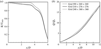
It is essential to show that the development of multiple jets is independent of the grid size and that of the physical domain. The instantaneous flow field has been computed using three different grid sizes, namely
 $190\times 240\times 240$
,
 $210\times 276\times 276$
and
 $240\times 360\times 360$
, for a domain size of
 $15D\times 25D\times 25D$
. The chosen grids are uniform in the streamwise direction and non-uniform in the spanwise direction. The uniform grids in the jet region are stretched in the two transverse directions so as to reduce the grid size in the outer domain where there are no changes in the flow field. The instantaneous vortical structures at
 $\mathit{Re}=2000$
,
 $A_{n}=5\,\%$
,
 $R/{\it\theta}=20$
and
 $\mathit{St}_{D}=0.5$
for these three grids did not show significant differences among the solutions. A direct comparison of the structures revealed that the simulations with differing grid resolution captured the formation of a blooming jet. The time-averaged centreline velocity and the normalized volumetric flow rate as functions of the axial distance are shown in figure 2 for the three grid sizes. The predictions of the intermediate and fine grids are seen to be quite close. Therefore, the results obtained using a grid size of
 $210\times 276\times 276$
are taken to be grid-independent, and this grid is used in the present study.
Variation of (a) the time-averaged streamwise velocity along the jet centreline and (b) the time-averaged volume flux normalized with the volume flux at the nozzle exit, for various frequency ratios;
 $\text{Reynolds number}=2000$
,
 $A_{n}=5\,\%$
,
 $R/{\it\theta}=20$
and
 $\mathit{St}_{D}=0.5$
; various computational grids are considered.

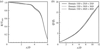
In view of the periodic nature of the boundary conditions at the transverse boundaries, the computed jet flow field is affected if a large enough transverse dimension is not chosen. Using periodic boundary conditions is equivalent to having flows created by an array of jets on the inflow boundary. The pitch of the periodicity is chosen in such a way that there is no effect of any of the jets on the evolution of the one under study. Therefore, the effect of the placement of periodic boundaries has been examined by performing calculations on various computational domains. Computations are carried out for three different transverse pitches, namely
 $25D$
,
 $30D$
and
 $40D$
, for a streamwise extent of
 $15D$
at a Reynolds number of 2000,
 $A_{n}=5\,\%$
,
 $R/{\it\theta}=20$
and
 $\mathit{St}_{D}=0.5$
. The corresponding grid sizes are
 $210\times 276\times 276$
,
 $210\times 302\times 302$
and
 $210\times 352\times 352$
respectively. The flow structures and their spatial evolution for the three domain sizes match well, indicating that a transverse domain size of
 $25D$
is sufficient to capture the physical spreading of the jet. The time-averaged centreline velocity and normalized volume flow rate are compared in figure 3 for the three domain sizes referred to above. The trends are seen to be quite close. Therefore, a pitch of
 $25D$
in the transverse direction has been selected for the placement of the periodic boundaries.
Variation of (a) the time-averaged streamwise velocity along the jet centreline and (b) the time-averaged volume flux normalized with the flux at the nozzle exit, for various frequency ratios; Reynolds number
 $=2000$
,
 $A_{n}=5\,\%$
,
 $R/{\it\theta}=20$
and
 $\mathit{St}_{D}=0.5$
; three computational domains are considered.

The influences of the time step and the initial conditions are discussed elsewhere (Gohil Reference Gohil2011). A typical dimensionless time-step size chosen for all the simulations is
 $10^{-4}$
, and the Courant–Friedrichs–Lewy (CFL) numbers are in the range of 0.05–0.2. The time step is to be compared with the time scale of order unity associated with Strouhal numbers in the range of 0.3–0.5.
Following da Silva & and Métais (Reference da Silva and Métais2002), the two confining surfaces transverse to the jet are modelled as periodic boundaries. Unlike these authors, however, a coflow boundary condition has not been used in the present study. Babu & Mahesh (Reference Babu and Mahesh2004) investigated the extent of entrainment by a jet (i) without coflow and (ii) with coflow arising from the use of a vanishing streamwise gradient of all components of velocity on the inflow plane outside the jet. In their study, no-slip boundary conditions were applied over the transverse confining surfaces. They did not observe any significant difference in the evolving flow field for their free evolving jet. Entrainment of the ambient fluid into the free jet is mainly radial. At the same time, the flow in the outer domain has to be replenished through an axial migration of the fluid opposite to the jet direction. Since the jet spreads with increasing entrainment in the downstream direction, the opposite motion of fluid in the outer domain ensures constant average velocity over the cross-section at any axial location and equal to the inlet value. Free-slip boundary conditions could have been used with transverse velocity being set to zero, instead of periodic boundary conditions. Numerical experiments show that the free-slip condition suppresses instability to a greater extent when compared with periodic conditions, and this condition has not been used in the present work. In addition, the locations of the transverse periodic boundaries have been selected to be large enough through numerical experimentation in such a way that the jet spreading is not size-dependent. With this choice of boundary conditions, both instabilities, namely helical and axisymmetric, are expected to grow spatially in a physically meaningful manner.
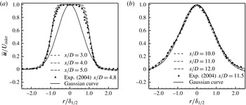
Validation of the DNS code for a free circular jet: velocity profiles in the near-orifice (
 $2\leqslant x/D\leqslant 5$
(a)) and far-orifice regions (
 $10\leqslant x/D\leqslant 12.0$
(b)) for a Reynolds number of 1030 compared with the experimental data of O’Neill, Soria & Honnery (Reference O’Neill, Soria and Honnery2004).

3.2. Validation
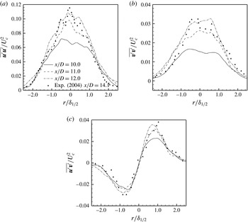
The computer code developed by the authors for the study of forced jets was first validated against the data of Wygnanski & Fiedler (Reference Wygnanski and Fiedler1969), Rodi (Reference Rodi1975), Panchapakesan & Lumley (Reference Panchapakesan and Lumley1993), Hussein, Capp & George (Reference Hussein, Capp and George1994) and O’Neill et al. (Reference O’Neill, Soria and Honnery2004) for unforced round jets. The comparison was found to be very good. Code validation for DNS as well as large-eddy simulations is discussed in detail in the previous work of the authors (Gohil et al. Reference Gohil, Saha and Muralidhar2011, Reference Gohil, Saha and Muralidhar2012, Reference Gohil, Saha and Muralidhar2013, Reference Gohil, Saha and Muralidhar2014). Figures 4 and 5 compare the present DNS calculation with the experimental results of O’Neill et al. (Reference O’Neill, Soria and Honnery2004) for a free circular jet. Time-averaged and statistical quantities in the two sets of results are seen to agree quite well. The instantaneous flows of the present simulation presented in a subsequent section for forced jets compare well qualitatively with the experimental flow visualization results of Lee & Reynolds (Reference Lee and Reynolds1985a ). Moreover, the time-averaged results for forced jets have also been compared wherever possible when discussing the results.
Validation of the DNS code for a free circular jet: Reynolds stress components in the far-orifice region for a Reynolds number of 1030 compared with the experimental data of O’Neill et al. (Reference O’Neill, Soria and Honnery2004).

4. Results and discussion
Instabilities in the evolution of a free circular jet and the appearance of large-scale structures have been discussed recently by the authors (Gohil et al.
Reference Gohil, Saha and Muralidhar2012). In an earlier work (Gohil et al.
Reference Gohil, Saha and Muralidhar2010), the authors showed the formation of Y- and
 ${\rm\Psi}$
-shaped bifurcations when the jet is perturbed by a flapping type of excitation. In the development of a circular jet, axisymmetric and helical instabilities play an important role and are jointly used in the present study to create dual-mode perturbation. This approach has been used by various authors in experiments (Lee & Reynolds Reference Lee and Reynolds1985b
; Parekh et al.
Reference Parekh, Leonard and Reynolds1988; Reynolds et al.
Reference Reynolds, Parekh, Juvet and Lee2003). A numerical approach to jet breakup using DNS at a Reynolds number of 2000 is discussed in the following sections. Small-scale perturbations are introduced at the inflow plane as Gaussian white noise with amplitude of 5 %, except in § 4.1.5 where different amplitudes are used to quantify its effect. The momentum thickness of the jet emerging into the ambient is kept fixed at 2.5 % of the jet diameter, except in § 4.1.3 which studies the influence of momentum thickness on jet breakup. Both instantaneous and the time-averaged flow fields are presented.
4.1. Instantaneous flow field
The present section is concerned with the effect of forcing parameters on the instantaneous flow field. The influences of the excitation frequency ratio, excitation frequency, initial momentum thickness, perturbation amplitude and small-scale perturbations are studied in the following sections.
4.1.1. Effect of excitation frequency ratio
Simulations show that the frequency ratio is an influential parameter for the formation of bifurcating and blooming jets. The frequency ratio can be tuned in such a way that the trajectory of an individual vortex ring is altered, thus spreading the flow in only one direction. The streamwise spacing between two consecutive vortex rings is realized in such a way that interactions between them are not possible over the computational domain.
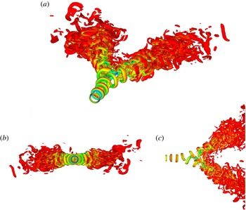
Figure 6 illustrates instantaneous vortical structures in terms of the
 $Q$
function in a bifurcating jet at a Reynolds number of 2000 and a frequency ratio of 2. Isosurfaces are coloured using the modulus of vorticity. Three different views show bifurcation on a particular plane, while no spreading is visible on the other plane. It is worth mentioning here that the choice of the bifurcating plane is dependent on the instant at which the perturbation is initiated and is controllable. Once the jet has bifurcated, each of the branches shows behaviour similar to a single jet. In addition, rapid augmentation of the entrainment rate of the external fluid into the core region is obtained.
Bifurcating jets at a Reynolds number of 2000 and a frequency ratio of 2: isosurfaces of
 $Q=0.1$
are shown in three different views for a circular jet,
 $\mathit{St}_{D}=0.5$
. The colour scale varies with the modulus of vorticity from blue (1) to red (6).

In the near field, laminar vortex rings tilt after travelling a short distance from the nozzle exit. Secondary structures develop in the intermediate region because of vortex stretching (figure 6). The interaction among various vortex structures causes the rings to lose coherence, resulting in fine-scale structures. Beyond the point of bifurcation, the core fluid between the two legs of the jet is stretched in the intermediate region where they are close to each other. The stretching of the fluid filaments enhances the mixing with the ambient fluid. The fluid element on the orthogonal plane is observed to be contracted especially in the immediate downstream vicinity of the initiation point of bifurcation. This could be due to the stretching of fluid elements on the bifurcating plane. Lee & Reynolds (Reference Lee and Reynolds1985a ) experimentally observed a similar bifurcation scenario using dual-mode perturbation at a frequency ratio of 2 and a Reynolds number of 4300 using laser-induced fluorescence (see also Reynolds et al. Reference Reynolds, Parekh, Juvet and Lee2003).
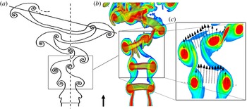
Vortex tilting in a row of non-concentric rings (a); superimposed vortical structures on the modulus of the vorticity in (b); a schematic drawing adapted from Reynolds et al. (Reference Reynolds, Parekh, Juvet and Lee2003) is shown in (c).

The physical mechanism of jet bifurcation can be described as follows. The axisymmetric part of the perturbation at the nozzle exit creates vortex rings. As these rings travel downstream, an uneven distribution of vorticity is obtained inside the rings due to helical perturbation. Hence, a variation in convective velocity is realized within a given vortex. The vortex ring tilts and generates self-induced velocity normal to its plane. For a frequency ratio of
 $R_{f}=2$
, consecutive vortex rings emerging from the nozzle exit are 180° out of phase. The movement of each of these vortex rings is along the resultant of the self-induced velocity and the streamwise convection velocity of the main flow. A closer view near the inception of bifurcation in figure 7(c) shows the modulus of the vorticity and the in-plane resultant velocity. When the resultant velocity is sufficiently large, the jet starts to bifurcate, splitting into two distinct parts. A similar bifurcation sequence has also been reported experimentally by Reynolds et al. (Reference Reynolds, Parekh, Juvet and Lee2003) (figure 7
a) where, along with the main vortex rings, secondary vortices in the form of ribs or braids connecting two consecutive vortex rings are also shown. The secondary vortices are generated due to stretching of the fluid between two consecutive rings. The results of numerical simulation reveal a similar distribution of secondary structures as well as flow evolution as conceived by Reynolds et al. (Reference Reynolds, Parekh, Juvet and Lee2003).
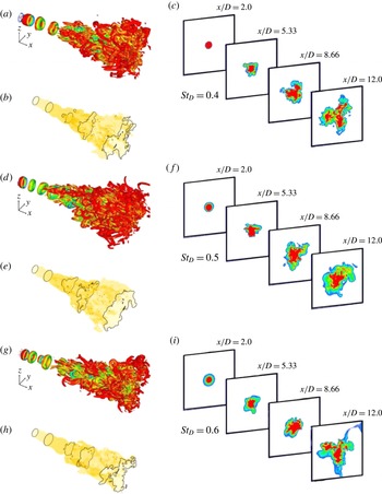
Trifurcating jets at a Reynolds number of 2000 and a frequency ratio of 3. (a,d,g) Isosurface of
 $Q=0.1$
; the colour scale varies with the modulus of vorticity from blue (1) to red (6). (b,e,h) Isosurface of instantaneous streamwise velocity (
 $u=0.1$
). (c,f,i) Contour plots of the streamwise velocity on cross-sectional planes at various
 $x/D$
locations for a circular jet.

Reynolds et al. (Reference Reynolds, Parekh, Juvet and Lee2003) suggested that a change in the excitation frequency ratio to 3 and 4 can divide the jet into three and four distinct branches respectively. To examine this proposal, simulation was independently performed at a lower Reynolds number of 2000 for combinations of axisymmetric and helical excitation with integer frequency ratios. The axisymmetric excitation frequency was varied from 0.4 to 0.6, while the excitation amplitudes were chosen to be between 2.5 % and 25 % of the peak velocity.
Figure 8 illustrates the effect of dual-mode perturbation with
 $R_{f}=3$
on the evolution of a circular jet. Despite momentary trifurcation, however, three distinct jets are not generated. In figure 8, isosurfaces of the
 $Q$
criterion show that circular vortex rings start to tilt in the near field due by dual-mode excitation. In the intermediate region, strong secondary vortices develop, and interaction of these vortices makes the flow structures complex. The formation of secondary vortices in the intermediate region makes it difficult to split the jet, although cross-sectional views at various axial sections show evidence of weak trifurcation. To see the effect of axial frequency on weak branching, computations were carried out using axisymmetric excitation frequencies (
 $\mathit{St}_{D}$
) of 0.4, 0.5 and 0.6. The contour plots of the streamwise velocity on cross-sectional planes at various
 $x/D$
locations for an axial frequency of 0.4 reveal the formation of trifurcation as compared with the other two frequencies (figure 8). At an axial frequency of 0.5, the jet exhibits spreading without any evidence of branching, while at a frequency of 0.6, the trifurcation nature in the cross-sectional planes is mildly preserved. Flow with a frequency ratio of
 $R_{f}=4$
is expected to develop four distinct branches. The present simulation did not show distinct branching, although interlinked branches were formed, as shown in figure 8. In summary, an integer frequency ratio of 2 led to clear bifurcation, but ratios of 3 and 4 did not to develop three and four distinct branches of the circular jet.
For irrational values of
 $R_{f}$
, when the axisymmetric perturbation frequency is an irrational multiple of the orbital frequency, Reynolds et al. (Reference Reynolds, Parekh, Juvet and Lee2003) stated that no vortex ring will exactly follow any other shed previously, and the jet can be made to bloom in an amazing shower of vortex rings. For a Reynolds number range of 2800–10 000, the authors predicted blooming jets for
 $1.5<R_{f}<3.2$
and
 $0.3<\mathit{St}_{D}<0.8$
. The mechanism of blooming is similar to that of a bifurcating jet, with the difference arising from the phases at which peaks of axisymmetric and helical perturbations match. For a bifurcating jet (
 $R_{f}=2$
), there are two phases per helical cycle, while for a blooming jet, the number of phases per helical cycle depends on the frequency ratio. The distance between two successive vortex rings thus depends on the frequency ratio.
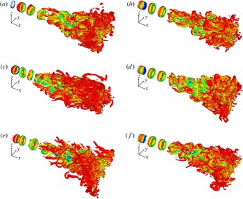
In a bifurcating jet, a single circular jet splits into two equal parts, thus dividing its mass flux into two halves. For a blooming jet, the question of the number of branches formed relative to the perturbation parameters needs to be addressed. Accordingly, simulations have been performed for various frequency ratios and amplitudes of perturbation. The axisymmetric excitation frequency is fixed at 0.4, which is the preferred mode frequency of a circular jet at the considered Reynolds number (Gohil et al. Reference Gohil, Saha and Muralidhar2011). The initial non-dimensional momentum thickness, random fluctuation level and amplitude of excitation are kept fixed at 2.5 %, 5.0 % and 15 % of the average velocity respectively. Figure 9 presents flow structures for frequency ratios between 1.3 and 3.4. Excitation frequency ratios of 1.65 and 2.4 show better spreading compared with the others. However, clear blooming is not observed.
Effect of frequency ratio: isosurfaces of
 $Q=0.1$
for a circular jet,
 $\mathit{St}_{D}=0.4$
and
 $\mathit{Re}=2000$
, for various frequency ratios,
 $R_{f}$
(1.3 (a), 2.4 (b), 1.65 (c), 2.8 (d), 1.8 (e), 3.4 ( f)). The colour scale varies with the modulus of vorticity from blue (1) to red (6).

The possibility of jet blooming for a given set of control parameters can be anticipated from the following discussion. Dual-mode excitation is a combination of axisymmetric and helical perturbations. Axial excitation encourages the formation of vortex rings and influences their strength. On the other hand, the perturbation frequency of the axial excitation determines the distance between two consecutive rings. The vorticity distribution over a given ring is affected by other rings in the neighbourhood through induced velocity. Thus, the effects of amplitude and frequency are coupled and will jointly affect the ring spacing.
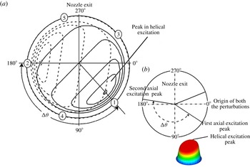
Schematic drawing explaining the idea of an offset angle (
 ${\rm\Delta}{\it\theta}$
).

The development of a tilted vortex ring is a direct consequence of the amplitude and frequency of the helical excitation. It arises from an uneven distribution of vorticity inside the ring, creating unequal induced velocities. When axisymmetric and helical perturbations are jointly present, one can imagine a wave moving along the circumference of the circular nozzle, giving rise to an uneven vorticity distribution over the vortex ring. Consequently, vortex rings move cyclically in various directions from distinct angular positions, giving an appearance of blooming.
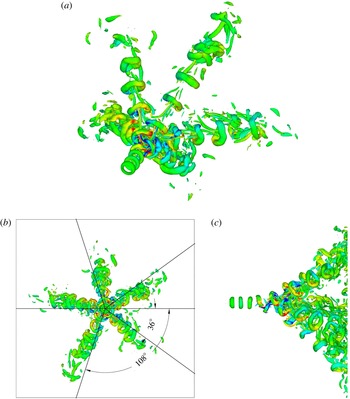
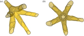
Isosurfaces of
 $Q=0.1$
in three different views for a forced circular jet. At
 $\mathit{St}_{D}=0.5$
,
 $R_{f}=2.5$
and
 $\mathit{Re}=2000$
, five distinct branches are seen at angles of 36°, 180°, 324°,
 $360^{\circ }+108^{\circ }$
and
 $360^{\circ }+252^{\circ }$
. The colour scale varies with the axial component of vorticity from blue (
 $-1$
) to red (1).

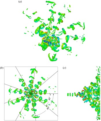
Isosurfaces of
 $Q=0.1$
in three different views for a forced circular jet. At
 $\mathit{St}_{D}=0.5$
,
 $R_{f}=2.25$
and
 $\mathit{Re}=2000$
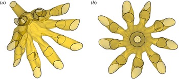
, nine distinct branches are seen at angles of 40°, 80°, 120°, 160°, 200°, 240°, 280°, 320° and 360°. The colour scale varies with the axial component of vorticity from blue (
 $-1$
) to red (1).

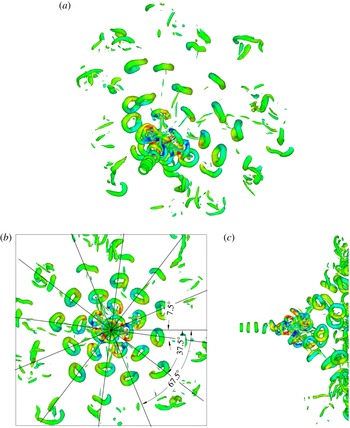
The joint effect of axisymmetric and helical perturbations is visualized in figure 10 for a frequency ratio of 2.5. The peak of the combined amplitudes of axisymmetric and helical perturbation fluctuates while rotating, as shown in figure 1. Figure 10(a) shows the contours of axial velocity fluctuations at the inflow plane for two time instants when the peaks of both the excitations match. The solid and broken contours reveal the variation of the helical perturbation at the above two instants. On the other hand, figure 10(b) represents the schematic of the instants when peaks in the axisymmetric perturbation occur. Here, the outer circle represents the boundary of the nozzle exit and 0° marks the initial phase of zero amplitude for each excitation. The initial phases (zero magnitude) of the two perturbations match in the simulations of the present study. All instants when the peaks of the excitations match are indicated by numbers, namely ‘1’, ‘2’, ‘3’, ‘4’ and ‘5’. The angle between the two consecutive peaks marked ‘1’ and ‘2’ is the offset angle (
 ${\rm\Delta}{\it\theta}$
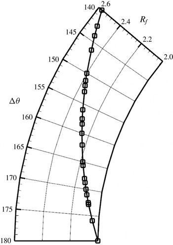
, in deg.). The first peak is expected at 36°, the second is at 180°, and so on. Therefore, the offset angle depends on the frequencies of the two excitations but not the amplitude. The offset angle can be related to the excitation frequency ratio as
 $$\begin{eqnarray}{\rm\Delta}{\it\theta}=\frac{360^{\circ }}{R_{f}}.\end{eqnarray}$$
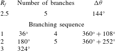
Equation (4.1) can be discussed in conjunction with figure 11, where an excitation frequency ratio of 2.5 develops a blooming jet with five branches. The offset angle is 144° and the first peak (point ‘1’) occurs at 36°. The total number of revolutions of the helical disturbance during which an axial cycle is completed is 2. Therefore, the total number of paths along which the vortex rings will move is
 $2\times 2.5=5$
. The sixth vortex ring will follow the same path as the first, and subsequent vortex rings will be displaced by the offset angle. As the time interval between two consecutive vortex rings in a particular path is large, the distance between them is large and removes the possibility of any interaction between them. However, there is a possibility of interaction between two rings of neighbouring branches. It is clear that a proper choice of frequencies is required to avoid such a possibility. Equivalently, blooming would be observed only for offset angles within a particular range. Table 1 summarizes the full sequence of shedding of vortex rings. After shedding of the first five vortex rings, the sixth ring follows the path of the first. Thus, table 1 suggests that the jet would bloom with five distinct branches.
Angular sequence of vortex branching when
 $R_{f}=2.5$
,
 $\mathit{Re}=2000$
and
 $\mathit{St}_{D}=0.5$
.

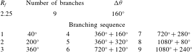
Angular sequence of vortex branching when
 $R_{f}=2.25$
,
 $\mathit{Re}=2000$
and
 $\mathit{St}_{D}=0.5$
.

Figure 11 shows isosurfaces of the
 $Q$
criterion function in three different views. It is clear from the figure that the jet blooms with five distinct branches appearing downstream. For a helical excitation frequency of 0.5, the shed vortex rings are moderately far apart and successively generated vortex rings do not interact with the preceding ones. Hence, the excitation frequency ratio controls the number of branches formed, while the applied helical perturbation controls the passage of the vortex rings, such that a newly formed ring is diverted into a particular branch. Since each branch is closely similar to the others, it is expected that the mass flow in any one of the branches is one-fifth of that leaving the nozzle. The angle between consecutive branches is estimated from an axial view of the vortical structures in figure 11. The first branch occurs at an angle of 36° from the zero phase of each excitation. The offset angle is measured to be 144°, and the angles of the other branches match those calculated in table 1. The simulation results corresponding to
 $R_{f}=2.25$
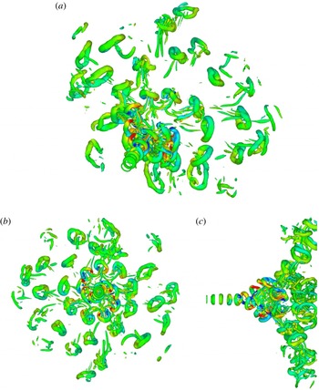
are presented in figure 12, while the vortex branching sequence is listed in table 2. The series of shedding angles suggests that nine distinct branches of the single circular jet are possible. The simulation data in figure 12 confirm this trend as well as the estimate of angles between consecutive branches.
Figure 12 can be compared with figure 11, where
 $R_{f}=2.5$
, generating five branches. The number of vortex rings in each branch is seen to diminish with increasing number of branches. For a frequency ratio of 2.25, a total of nine axial cycles is completed in four helical cycles, resulting in a longer time interval between two successive rings. Specifically, the wavelength between consecutive vortex rings increases with a reduction in frequency ratio. With greater separation between vortex rings, secondary vortices are delayed, thus making the flow quite regular. In addition, the effective Reynolds number for each branch is lower by a factor equal to the number of branches. This finding can be used to control the onset of turbulence in a jet.
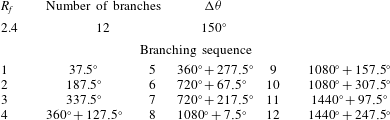
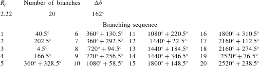
The above discussion can be extended to frequency ratios of 2.4 and 2.22, where the offset angles are 150° and 162°. The vortex branching sequences for these perturbations are listed in tables 3 and 4. The jet blooms with 12 and 20 branches for excitation frequencies of 2.4 and 2.22 respectively. These expectations are brought out through simulations. A confirmation of the branching sequence for
 $R_{f}=2.4$
is shown in figure 13. Lee & Reynolds (Reference Lee and Reynolds1985a
) carried out smoke visualization studies for
 $R/{\it\theta}=20$
,
 $\mathit{St}_{D}=0.5$
,
 $R_{f}=2.4$
and
 $\mathit{Re}=4300$
. Both studies show branches generated due to the successively generated circular vortex rings as they follow independent paths, as stipulated by the frequency ratio. A comparison of the present computations with experiments reveals an excellent match in terms of jet branching and the location point of the inception of the branching, even though the two studies are at different Reynolds numbers.
Isosurfaces of vortical structures in three different views are shown in figures 13 and 14 for excitation frequency ratios of 2.4 and 2.22 respectively. Multiple branches are visible, while the gap between consecutive vortex rings in a branch increases for increasing number of branches. For
 $R_{f}=2.22$
, the number of branches is 20, and vortices between adjacent branches interact and create secondary vorticity. The development of hairpin-like secondary vortices is now related to the close proximity of the branches. For five branches, the angle between two of them is 72°. This reduces to 40°, 30°and 18° as the number of branches increases from nine to 12 to 20 respectively. The vortex strength decreases for a greater number of branches because of mass division and the formation of secondary vortices. As they travel downstream, the vortices further lose circulation by viscous diffusion, causing each one to have lower peak vorticity.
Angular sequence of vortex branching when
 $R_{f}=2.4$
,
 $\mathit{Re}=2000$
and
 $\mathit{St}_{D}=0.5$
.

Angular sequence of vortex branching when
 $R_{f}=2.22$
,
 $\mathit{Re}=2000$
and
 $\mathit{St}_{D}=0.5$
.

Isosurfaces of
 $Q=0.1$
in three different views for a forced circular jet. At
 $\mathit{St}_{D}=0.5$
,
 $R_{f}=2.4$
and
 $\mathit{Re}=2000$
, twelve distinct branches are seen at angles of 37.5°, 67.5°, 97.5°, 127.5°, 157.5°, 187.5°, 217.5°, 247.5°, 277.5°, 307.5° and 337.5°. The colour scale varies with the axial component of vorticity from blue (
 $-1$
) to red (1).

Isosurfaces of
 $Q=0.1$
in three different views for a forced circular jet. The step size of the
 $Q$
criterion function is 0.1. At
 $R_{f}=2.22$
and
 $\mathit{Re}=2000$
, 20 distinct branches are formed. The colour scale varies with the axial component of vorticity from blue (
 $-1$
) to red (1).

Graphical representation of the dependence of the offset angle on the excitation frequency ratio within the parameter range that generates 2–50 branches.

At lower frequency ratios (figure 9), the jet has not shown evidence of blooming and (4.1) is not applicable. This observation suggests that blooming would be seen for frequency ratios falling within a certain range. For
 $R_{f}=2$
, two distinct branches are seen, the offset angle of 180° being consistent with (4.1). This frequency ratio can be taken as a lower limit for jet branching. To establish an upper limit of the excitation frequency, figures 9–12 (and tables 1–4) can be examined. The upper limit of the frequency ratio is reached when the combined effect of tilting of vortex rings with respect to the jet centreline and the distance between two vortex rings delays collapse of the ring vortices and allows the jet to bloom. The appropriate offset angles fall in the range
 $140^{\circ }<{\rm\Delta}{\it\theta}<180^{\circ }$
, corresponding to an excitation frequency ratio interval of
 $2<R_{f}<2.6$
. The polar representation connecting the offset angle with the frequency ratio is shown in figure 15.
4.1.2. Effect of axisymmetric excitation frequency
In the previous section, the axisymmetric excitation frequency was kept at a constant value of
 $\mathit{St}_{D}=0.5$
, while the frequency ratio was varied, leading to a change in the helical excitation frequency,
 $\mathit{St}_{H}$
. The present section deals with the effect of the frequency of the axisymmetric perturbation on the blooming phenomenon at an excitation frequency ratio of
 $R_{f}=2.4$
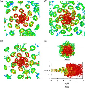
. The four frequencies chosen are
 $\mathit{St}_{D}=0.45$
, 0.50, 0.525 and 0.55 for a Reynolds number of 2000. Other parameters specified are
 $A_{n}=5\,\%$
and inlet shear layer thickness,
 $R/{\it\theta}=20$
.
Effect of axial excitation frequency: axial view of isosurfaces of
 $Q=0.1$
for a forced circular jet. At
 $R_{f}=2.4$
and
 $\mathit{Re}=2000$
, 12 distinct branches are formed. The colour scale varies with the axial component of vorticity from blue (
 $-0.5$
) to red (0.5): (a)
 $\mathit{St}_{D}=0.45$
, (b)
 $\mathit{St}_{D}=0.525$
, (c)
 $\mathit{St}_{D}=0.5$
, (d)
 $\mathit{St}_{D}=0.55$
.

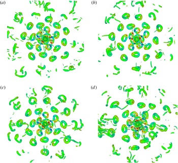
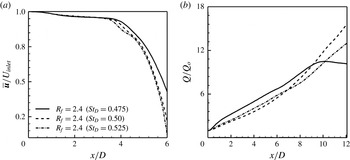
Figure 16 shows the formation of instantaneous vortical structures for various frequencies. It is clear that an axisymmetric excitation frequency in the range 0.45–0.525 shows the formation of 12 branches and confirms the possibility of achieving the blooming effect. However, differences are seen in the structures formed at various frequencies. With increasing excitation frequency, the number of vortex rings increases. Consequently, the distance between two consecutive rings decreases in any branch. This is because with increasing excitation frequency, the time interval available for advection of any ring in a branch decreases. The axial view of the vortical structures is shown in figure 16(d) for an axisymmetric excitation frequency of 0.55. Here, the jet fails to bloom and is unable to spread.
The side view of the vortical structures of the instantaneous field is also shown in figure 16(d). In the near field, the distance between two consecutive vortex rings is small, and successive vortex rings interact with one another in the intermediate region of the jet. Secondary structures are created and prevent the jet from blooming. The spreading of the circular jet is diminished in the radial direction. At the limit of the lowest frequency, vortex rings are too far apart to undergo blooming before they break down by other instability mechanisms.
The discussion related to figure 16 at a frequency ratio of 2.4 suggests that the working range of the axisymmetric excitation frequency for which there is a possibility of blooming of jets is
 $0.45<\mathit{St}_{D}<0.525$
. This range covers the preferred frequency of the jet that triggers natural transition. Reynolds et al. (Reference Reynolds, Parekh, Juvet and Lee2003) suggested a frequency range of 0.3–0.8 for axisymmetric perturbation resulting in blooming jets. The present study narrows this range down further.
4.1.3. Effect of inlet momentum thickness
The effect of inlet momentum thickness on the evolution of a blooming jet was studied with four
 $R/{\it\theta}$
ratios, namely 20, 40, 60 and 90. Other computational parameters were fixed at an excitation frequency ratio of
 $R_{f}=2.4$
, an excitation frequency of 0.5 and an excitation amplitude
 $=5\,\%$
, while the jet Reynolds number was 2000. As
 $R/{\it\theta}$
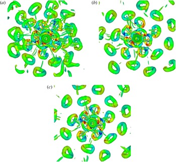
increases, the shear layer becomes thinner at the inflow plane of the jet. Figure 17 shows the axial view of the isosurfaces of vortical structures for the parameters considered. A comparison of the instantaneous fields in the figure suggests that the development of a blooming jet as well as the formation of a number of branches is not sensitive to the initial momentum thickness.
Effect of inlet momentum thickness: isosurfaces of
 $Q=0.1$
as seen along the axis of a forced circular jet;
 $\mathit{Re}=2000$
and
 $\mathit{St}_{D}=0.5$
. At
 $R_{f}=2.4$
, 12 distinct branches are formed. The colour scale varies with the axial component of vorticity from blue (
 $-1$
) to red (1): (a)
 $R/{\it\theta}=20$
, (b)
 $R/{\it\theta}=60$
, (c)
 $R/{\it\theta}=40$
, (d)
 $R/{\it\theta}=90$
.

For a free turbulent jet, Gutmark & Ho (Reference Gutmark and Ho1983) have shown that the Strouhal number defined on the basis of the inlet momentum thickness of the shear layer is a constant, indicating a dependence of the frequency on the momentum thickness. Closer to the nozzle, the spacing of the vortex rings in the forced jet is large enough to prevent generation of secondary flow. Further, the Reynolds number of the branching jets is small and, hence, the overall flow is expected to be laminar. In addition, the power spectra of the streamwise velocity component prior to branching consistently showed a definite peak at the forcing frequency without any signature of the inlet momentum thickness.
4.1.4. Effect of perturbation amplitude
Apart from the excitation frequency, a parameter quoted in active flow control is the excitation amplitude. It relates directly to the power required to influence the main flow field. In experiments, amplitudes as high as 15 % of the average inlet velocity have been utilized. Numerical studies in the literature start with amplitudes as small as 5 %. In the present work, the effect of the excitation amplitude is discussed parametrically with respect to blooming of a forced jet. Three excitation amplitudes, namely 2.5 %, 5.0 % and 7.5 %, have been used for this purpose. Other parameters in the study are Reynolds number
 $=2000$
,
 $R/{\it\theta}=20$
,
 $\mathit{St}_{D}=0.5$
and
 $R_{f}=2.4$
.
Figure 18 presents the isosurfaces of the vortical structures in terms of the
 $Q$
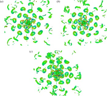
function at various excitation amplitudes. Even at the lowest excitation amplitude of 2.5 %, clear blooming of the jet with 12 distinct branches is visible.
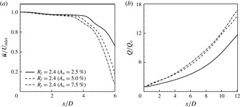
A comparison of the flow structures for the three amplitudes reveals a few differences. With an increase in excitation amplitude, the strength of the vortex ring increases and causes a distinct ring to form. Vortices of higher strength induce larger self-induced velocities. The distance between two rings in a branch then tends to increase with increasing amplitude of excitation. As a result, fewer secondary structures are generated, and clear vortex rings propagate longer distances in the flow field. In addition, stronger vortex rings increase the overall entrainment of the external fluid into the jet core and, consequently, jet spreading. Figure 18, however, shows that excitation amplitude is not a deciding parameter for the jet to bloom.
Effect of perturbation amplitude: isosurfaces of
 $Q=0.1$
seen along the axis of a circular jet;
 $\mathit{Re}=2000$
and
 $\mathit{St}_{D}=0.5$
. At
 $R_{f}=2.4$
, 12 distinct branches are formed. The colour scale varies with the axial component of vorticity from blue (
 $-1$
) to red (1): (a)
 $A_{n}=2.5\,\%$
, (b)
 $A_{n}=5\,\%$
, (c)
 $A_{n}=7.5\,\%$
.

Effect of small-scale perturbation: isosurfaces of
 $Q=0.1$
seen along the axis of a circular jet;
 $\mathit{Re}=2000$
,
 $A_{n}=5\,\%$
and
 $\mathit{St}_{D}=0.5$
. At
 $R_{f}=2.4$
, 12 distinct branches are clear. The colour scale varies with the axial component of vorticity from blue (
 $-1$
) to red (1): (a)
 $W_{n}=0.0\,\%$
, (b)
 $W_{n}=0.5\,\%$
, (c)
 $W_{n}=5.0\,\%$
.

4.1.5. Effect of small-scale perturbation
In addition to the momentum thickness, the inlet small-scale perturbation intensity is a parameter governing the behaviour of free and forced jets. Although the Reynolds number is fixed in the present simulation at 2000, the perturbation intensity can change from one experimental apparatus to another. The small-scale perturbation is generated from a sequence of random numbers that have a Gaussian probability density function (PDF). The corresponding spectrum is broadband and the energy content corresponding to the preferred mode is small. In contrast, the large-scale perturbation is organized, and will have substantial energy at the correct frequency to disturb the jet and make it bloom.
To quantify the effect of random small-scale perturbation on the inflow plane, three perturbation intensities, namely 0 %, 0.5 % and 5 %, have been used. Other parameters held fixed are Reynolds number
 $=2000$
,
 $R/{\it\theta}=20$
,
 $A_{n}=5.0\,\%$
,
 $\mathit{St}_{D}=0.5$
and
 $R_{f}=2.4$
. In the simulations, small-scale perturbation in the form of Gaussian noise is applied to the three velocity components in addition to the large-scale perturbation as per (3.3).
Figure 19 shows the isosurfaces of the vortical structures in the axial view as a function of the small-scale perturbation intensity. The flow field reveals blooming of the jet with 12 distinct branches. It is clear that blooming is barely sensitive to the inflow conditions. There could be a quantitative impact of inlet small-scale perturbations on factors such as entrainment, and these are examined from the time-averaged field, § 4.2.
4.2. Time-averaged flow field
The instantaneous flow patterns show dramatic enhancement of the jet spreading when dual-mode excitation is used at the nozzle exit. It is of interest to examine the branching of jets in the time-averaged sense. The time-averaged flow field along with velocity profiles helps in quantifying important parameters such as the entrainment rate and spreading. Time averaging was performed with data generated over 200–250 cycles of axisymmetric excitation. The initial 75 cycles were neglected in order to allow the transients to settle in the flow field.
Discussions related to the instantaneous flow field suggest that the excitation frequency ratio has a strong effect on the formation of multiple branches of a circular jet. Hence, the time-averaged flow field is analysed for excitation frequency ratios of
 $R_{f}=2$
, 2.5, 2.25 and 2.4. Figure 20 shows isosurfaces of the time-averaged streamwise velocity in various views at
 $R_{f}=2$
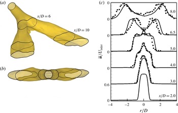
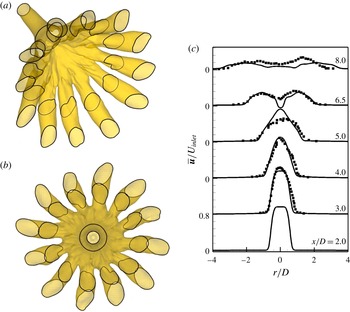
, where the formation of two branches is visible. The closed black curves show jet sections at various streamwise locations indicating the formation of multiple branches. The sectional plane is located at a particular axial location. The intersection of the sectional plane with the isosurface of the streamwise velocity generates a closed curve. The locations of the sectional plane are incorporated in figure 20. The closed curves confirm that the bifurcation phenomenon is preserved in the time-averaged field.
(a,b) Isosurfaces of the time-averaged streamwise velocity (
 $u=0.1$
) in two views for a bifurcating circular jet;
 $\mathit{Re}=2000$
,
 $A_{n}=5\,\%$
,
 $R/{\it\theta}=20$
and
 $\mathit{St}_{D}=0.5$
. At
 $R_{f}=2$
, two distinct branches are formed. (c) Time-averaged velocity profiles for a bifurcating jet on a bifurcating plane. The present data are shown by a smooth curve (
 $\mathit{Re}=2000$
), and the square symbols show the experimental data of Lee & Reynolds (Reference Lee and Reynolds1985a
) (
 $\mathit{Re}=4300$
).

According to Parekh et al. (Reference Parekh, Leonard and Reynolds1988), a jet that spreads more rapidly in one plane than in the perpendicular plane is not necessarily a bifurcating jet, since elliptic jets exhibit similar characteristics. Based on flow visualization, they proposed two criteria to define a bifurcating jet: the jet splits into two and/or the far-field streamwise velocity profile consists of two distinct peaks.
A comparison of the computed time-averaged velocity field with the experimental results of Lee & Reynolds (Reference Lee and Reynolds1985a
) on bifurcating and bisecting planes at various streamwise locations is presented here. Lee & Reynolds (Reference Lee and Reynolds1985a
) used an excitation frequency of 0.46, a frequency ratio of 2 and a Reynolds number of 4300. However, for the present study, the jet parameters are
 $\mathit{St}_{D}=0.5$
,
 $A_{n}=5.0\,\%$
and
 $\mathit{Re}=2000$
, although the frequency ratio,
 $R_{f}$
, is equal to 2. Despite differences in the Reynolds number and the excitation frequency, figure 20(c) reveals that the comparison is excellent for the near-field data. Until
 $x/D=5$
, the time-averaged velocity distribution does not show evidence of bifurcation. However, at
 $x/D=6.5$
, two distinct peaks in the velocity are visible. The magnitudes of the peak velocity in simulation and experiments are nearly equal. A slight variation in the radial spreading of the jet is observed at
 $x/D=8.0$
.
Isosurfaces of the time-averaged streamwise velocity (
 $u=0.1$
) in two views for a blooming circular jet;
 $\mathit{Re}=2000$
,
 $A_{n}=5\,\%$
,
 $R/{\it\theta}=20$
and
 $\mathit{St}_{D}=0.5$
. At
 $R_{f}=2.5$
, five distinct branches are formed.

At an excitation frequency ratio of 2.5, the instantaneous flow field shows the development of five distinct branches. The isosurfaces of the time-averaged streamwise velocity in figure 21 also reveal five branches originating from a single circular jet. The angle between any two consecutive branches is 72°, as reported for the instantaneous flow field.
Isosurfaces of the time-averaged streamwise velocity (
 $u=0.1$
) in two views for a blooming circular jet;
 $\mathit{Re}=2000$
,
 $A_{n}=5\,\%$
,
 $R/{\it\theta}=20$
and
 $\mathit{St}_{D}=0.5$
. At
 $R_{f}=2.25$
, nine distinct branches are formed.

For
 $R_{f}=2.25$
, figure 22 shows that the time-averaged flow field has developed nine branches. Similarly, figure 23 illustrates the formation of 12 branches at
 $R_{f}=2.4$
. The computed time-averaged flow field is also compared with the experimental results of Lee & Reynolds (Reference Lee and Reynolds1985a
) in figure 23(c) for
 $R_{f}=2.4$
and an excitation frequency of
 $\mathit{St}_{D}=0.5$
. The numerical simulation adopts a Reynolds number of 2000, while Lee & Reynolds (Reference Lee and Reynolds1985a
) used
 $\mathit{Re}=4300$
. Figure 23(c) shows a good comparison between the two sets of data over the physical domain of interest. At
 $x/D=8$
, the velocity profiles on the bifurcating plane become flat, indicating strong jet spreading in the radial direction.
(a,b) Isosurfaces of the time-averaged streamwise velocity (
 $u=0.1$
) in two views. (c) Time-averaged streamwise velocity profiles of a blooming circular jet;
 $\mathit{Re}=2000$
,
 $A_{n}=5\,\%$
,
 $R/{\it\theta}=20$
and
 $\mathit{St}_{D}=0.5$
. At
 $R_{f}=2.4$
, 12 distinct branches are formed. The simulation data are shown by a smooth curve (
 $\mathit{Re}=2000$
), and the square symbols show the experimental data of Lee & Reynolds (Reference Lee and Reynolds1985a
) (
 $\mathit{Re}=4300$
).

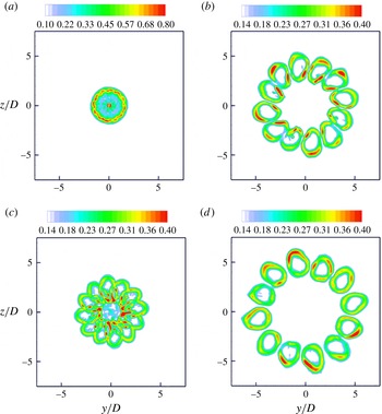
The contour plots of the modulus of the time-averaged vorticity on a cross-section plane (
 $y{-}z$
) at four axial locations,
 $x/D=6$
, 8, 10 and 12, are shown in figure 24. At
 $x/D=6$
, the signature of branches, although visible, is not distinct. Further downstream (
 $x/D=8$
), 12 branches can be clearly observed. The increasing distances among the twelve lobes from the centreline confirm the spreading of the jet. An examination of the contour levels at various locations reveals that the vorticity magnitude decays with distance, as expected. Moreover, the spreading of the individual branch jet is also clearly seen from the increasing size with increasing downstream distance.
Contour plots of the time-averaged modulus of vorticity (
 $|\bar{{\it\omega}}|$
) on cross-sectional planes of a blooming circular jet;
 $\mathit{Re}=2000$
,
 $A_{n}=5\,\%$
,
 $R/{\it\theta}=20$
,
 $\mathit{St}_{D}=0.5$
and
 $R_{f}=2.4$
; (a)
 $X/D=6$
, (b)
 $X/D=10$
, (c)
 $X/D=8$
, (d)
 $X/D=12$
.

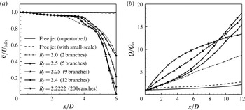
In order to measure quantitatively the spreading rates and entrainment in the bifurcating and blooming jets, the time-averaged streamwise velocity variation along the jet centreline for various excitation frequency ratios is compared with that for free jets. Figure 25(a) shows the effect of large-scale perturbation in the far field of the jet. The free jet shows similar variation with and without random small-scale perturbation. However, with dual-mode excitations, dramatic enhancement in the velocity decay is observed. Thus, improvement in jet spreading is obtained downstream. As the jet experiences bifurcation at
 $R_{f}=2$
, it starts to spread at
 $x/D\approx 2$
due to the formation of vortex rings. Spreading due to jet bifurcation becomes effective beyond
 $x/D\approx 5$
. As the number of branches increases, the centreline velocity progressively decreases. Hence, considerable improvement in spreading is obtained for a blooming jet.
An interesting property of the time-averaged flow is the volume flow rate
 $Q(x)$
associated with the jet, which is defined as
 $$\begin{eqnarray}Q(x)=\int _{0}^{\infty }\int _{0}^{\infty }\bar{u}(y,z)\,\text{d}y\,\text{d}z.\end{eqnarray}$$
Variation of (a) the time-averaged streamwise velocity and (b) the time-averaged volume flux, normalized with the flux at the nozzle exit, along the jet centreline for various frequency ratios at a Reynolds number of 2000,
 $A_{n}=5\,\%$
,
 $R/{\it\theta}=20$
and
 $\mathit{St}_{D}=0.5$
.

Its derivative with respect to the axial location provides a quantitative estimate of entrainment. The normalized volume flow rate
 $Q/Q_{o}$
data are presented in figure 25(b); here,
 $Q_{o}$
is the jet exit volume flow rate. The free jet shows a weak entrainment rate even far downstream. With the addition of small-scale random perturbation, a slight improvement in the entrainment rate is observed. However, dual-mode excitation increases the entrainment rate dramatically both in the near field as well as far downstream.
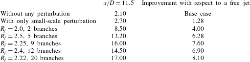
A precise assessment of the entrainment of the external fluid into the jet is reported in table 5 for
 $x/D=11.5$
and various excitation frequency ratios. Table 5 also presents the improvement in entrainment of bifurcating and blooming jets over a free jet. The addition of the small-scale random perturbation shows performance improvement by a factor of 1.28. At an excitation frequency ratio of 2, the circular jet bifurcates and the improvement in the entrainment is a factor of 4. In blooming jets with five branches, the performance increase is a factor of 6.28. As expected, the greatest performance enhancement of 8.1 is obtained for an excitation frequency ratio of 2.22 with 20 branches.
Apart from the excitation frequency ratio (
 $R_{f}$
), the instantaneous flow field shows that the axisymmetric excitation frequency and amplitude play a significant role in jet spreading. Blooming jets are formed for
 $\mathit{St}_{D}$
in the range of 0.45–0.525. To quantify the spreading of a blooming jet, the time-averaged data for three axial frequencies at
 $R_{f}=2.4$
are reported in figure 26. Increase in spreading is seen in the time-averaged data. The time-averaged streamwise velocity along the jet centreline decreases rapidly with increasing axisymmetric excitation frequency (figure 26
a).
Variation of (a) the time-averaged streamwise velocity and (b) the time-averaged volume flux, normalized with the flux at the nozzle exit, along the jet centreline for various axial perturbation frequencies at a Reynolds number of 2000,
 $R_{f}=2.4$
,
 $A_{n}=5\,\%$
and
 $R/{\it\theta}=20$
.

The variation of the normalized volume flow rate
 $Q/Q_{o}$
along the jet centreline shown in figure 26(b) shows the entrainment to be a maximum for an excitation frequency of 0.5 as compared with the other two values considered. For a frequency of 0.475, the jet performance has degraded downstream, with the flow rate becoming nearly a constant.
Three amplitudes of large-scale excitation have also been studied while keeping other controlling parameters constant. Figure 27 illustrates a rapid decay of velocity along the jet centreline and the variation of the normalized volume flux with increasing downstream distance for various excitation amplitudes. The decay of the velocity arises from stronger vortices created by higher excitation amplitude. This results in weaker secondary structures, and the blooming effect is sustained over a longer distance. With increasing excitation amplitude, the velocity distribution suggests that jets bloom early and spreading starts closer to the nozzle exit. As the excitation amplitude increases, the entrainment of the external fluid into the jet increases, although the difference between entrainment rates of 5 % and 7.5 % is only marginal.
Variation of (a) the time-averaged streamwise velocity and (b) the time-averaged volume flux, normalized with the flux at the nozzle exit, along the jet centreline for various amplitudes at a Reynolds number of 2000,
 $R_{f}=2.4$
,
 $R/{\it\theta}=20$
and
 $\mathit{St}_{D}=0.5$
.

Improvement in entrainment over a free unperturbed circular jet by inlet plane forcing.

5. Conclusions
The possibility of increasing the spreading rate of a circular jet by inlet plane perturbations has been examined at a Reynolds number of 2000 using DNS. Bifurcating and blooming jets are achieved through dual-mode forcing, namely a combination of axisymmetric and helical excitation. The properties of the forced jet are studied as a function of the excitation frequency ratio, axisymmetric frequency, excitation amplitude and amplitude of small-scale disturbances.
The present study shows that a circular jet can be divided by a suitable choice of forcing parameters. Among these,
 $R_{f}$
, the frequency ratio of the perturbation modes, plays an important role in fixing the number of branches formed. An excitation frequency ratio of 2 results in bifurcation. The blooming phenomenon is seen only for non-integer frequency ratios. For ratios of 2.5, 2.25, 2.4 and 2.22, a single circular jet divides into 5, 9, 12 and 20 branches respectively. The appropriate frequency ratio falls in the range
 $2<R_{f}<2.6$
, corresponding to offset angles of
 $140^{\circ }<{\rm\Delta}{\it\theta}<180^{\circ }$
. These trends are marginally influenced by the inlet shear layer thickness, the initial small-scale perturbation level and, within limits, the excitation amplitude. The above observations have been found to be applicable for the axisymmetric excitation frequency in the range of
 $0.45<\mathit{St}_{D}<0.525$
.
The time-averaged flow field is consistent with the instantaneous description and shows the development of blooming jets. The effect of blooming is most prominently seen in the entrainment ratio, which can be as high as a factor of 8 over a free jet, for 20 branches.
Acknowledgement
The authors gratefully acknowledge the High Performance Computing Facility available at Indian Institute of Technology Kanpur which enabled the large-scale computations reported here.