1 Introduction
The focus of the present study is to investigate the dominant physical effects at resonance for moonpools with recess. A recess is the water above an intermediate working deck in a moonpool (referred to as the ‘recess floor’ in this paper). This is considered as an alternative to working on the object on the main deck, and has recently gained increased attention. The present study involves numerical, analytical and experimental investigations of two-dimensional moonpools with recess in forced heave and surge conditions. Due to the asymmetry introduced by the recess, sloshing modes are induced also by heave motions. Damping due to flow separation and nonlinearities due to interaction between recess and free surface are expected. Experimental and numerical studies are performed in a two-dimensional setting, where a moonpool configuration is forced to heave with different periods and amplitudes. Molin (Reference Molin2017) observed a change in the mode shapes due to the presence of the recess, which motivated the present study, where we investigate the piston and first sloshing mode shapes experimentally. Main findings include the importance of viscous damping around the first sloshing mode, mainly caused by flow separation at the recess top corner. Nonlinear effects of the free-surface elevation at the first sloshing mode at relatively large amplitudes of motion are also discussed.
Several authors have studied the traditional moonpools without recess, referred to as clean moonpools in this paper. Molin (Reference Molin2001) studied the resonance problem for the clean moonpool by means of the domain-decomposition method assuming linear potential flow theory. Faltinsen, Rognebakke & Timokha (Reference Faltinsen, Rognebakke and Timokha2007) developed a two-dimensional (2-D) solution based on Green’s function for clean moonpools. They obtained solutions for both the moonpool response and linear hydrodynamic coefficients. Two-dimensional studies in forced heave are presented by Kristiansen (Reference Kristiansen2009), Kristiansen & Faltinsen (Reference Kristiansen and Faltinsen2012), Fredriksen, Kristiansen & Faltinsen (Reference Fredriksen, Kristiansen and Faltinsen2015). These studies show that the viscous damping is dominant at the piston mode resonance for clean moonpools. The viscous damping arises due to flow separation at the sharp corners of the moonpool inlet. When a recess is introduced, additional effects from flow separation at the recess corner are expected. Further, depending on the recess dimensions, free-surface nonlinearities may become important. Kristiansen & Faltinsen (Reference Kristiansen and Faltinsen2012) developed a hybrid method for numerical calculation of the response in moonpools by means of a combination of Navier–Stokes and potential flow solvers. The idea was to include the effect of flow separation, while at the same time perform time-efficient simulations. In the present work, we implement this method, and discuss its applicability for moonpools with recess.
Recently, Molin (Reference Molin2017) expanded the theory in Molin (Reference Molin2001) to moonpool configurations with recess in deep water and the three-dimensional flow field outside the moonpool. These methods provide the natural periods and corresponding mode shapes for the free surface in the moonpool. The methods involve solving an eigenvalue problem, and do not predict the amplitude of the free-surface motion. Similar work was done in Newman (Reference Newman2018), where Legendre polynomials were used instead of Fourier functions. By using Legendre polynomials, the added mass coefficients were calculated analytically, in addition to the natural frequencies. Zhang, Huang & Song (Reference Zhang, Huang and Song2019) developed a method for determining natural frequencies and modal shapes of the free surface of two-dimensional asymmetric and symmetric moonpools in finite water depth by using a domain-decomposition method. The method is applicable for side-by-side operations of vessels with two different dimensions. In the present work, we extend the methods for two-dimensional moonpools with one or two recesses in finite water depth.
The paper is organized as follows: a domain-decomposition method for predicting the natural frequencies, and corresponding mode shapes of the free surface, is developed in § 2. In § 3 the numerical methods are presented, and the experimental set-up is discussed in § 4. Finally, § 5 presents and discusses the results from the experimental and numerical studies, followed by conclusions in § 6.
2 Domain-decomposition method
A domain-decomposition (DD) method is developed to determine the natural frequencies of the resonant modes in a two-dimensional moonpool with recess for a vessel in finite depth. This is a continuation of the methods described in Molin (Reference Molin2017) for moonpools with a three-dimensional flow field outside the moonpool in deep water and two-dimensional in the moonpool, where the present method considers two-dimensional flow in the whole domain and finite water depth. Linear potential flow theory is assumed. Based on matched eigenfunction expansions, the fluid domain is divided into three subdomains. The method predicts the natural frequencies and the corresponding mode shapes of the free surface in the moonpool.
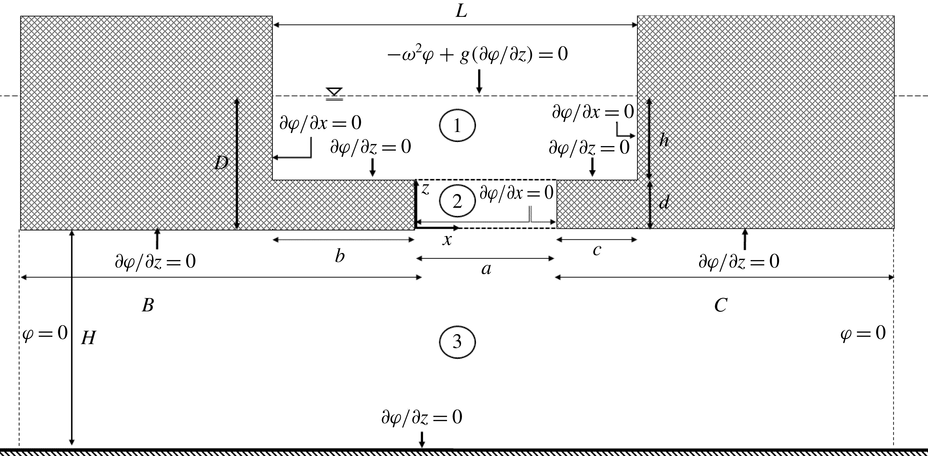
The boundary value problem is presented in figure 1. The present DD method allows for two recesses. Analytic expressions for the velocity potentials in the three domains are given in (A 1), where they satisfy the Laplace equation (
 $\unicode[STIX]{x1D6FB}^{2}\unicode[STIX]{x1D719}=0$
) and homogenous Neumann conditions for
 $\unicode[STIX]{x1D719}$
at the walls. The pressure and the normal velocities, i.e. velocity potentials and their vertical derivatives, are matched at the boundaries. The details of the derivation are given in appendix A.
The natural frequencies
 $\unicode[STIX]{x1D714}_{n}$
, with
 $n=0,1,\ldots ,\infty$
, are the solutions to (A 7). The natural frequencies are predicted with a precision of four significant digits with
 $N=25$
, where
 $N$
is the number of terms in the series in (A 1).
Boundary value problem for the domain-decomposition method with three subdomains, for determination of natural frequencies
 $\unicode[STIX]{x1D714}_{n}$
,
 $n=0,1,\ldots ,\infty$
.

3 Numerical methods
Numerical simulations are conducted with and without accounting for viscous effects. The latter is obtained by means of a time-domain boundary element method (BEM) code implemented herein, based on linearized potential flow theory. The former is obtained with approximate solutions of the Navier–Stokes equations combined with linearized free-surface and body-boundary conditions as in Kristiansen & Faltinsen (Reference Kristiansen and Faltinsen2012), referred to as CFD here.
3.1 Boundary element method
We assume that the water is incompressible and inviscid, and that the flow is irrotational. There exists a velocity potential,
 $\unicode[STIX]{x1D719}$
, such that
 $\boldsymbol{u}=\unicode[STIX]{x1D735}\unicode[STIX]{x1D719}$
in
 $\unicode[STIX]{x1D6FA}$
:
 $\unicode[STIX]{x1D6FA}$
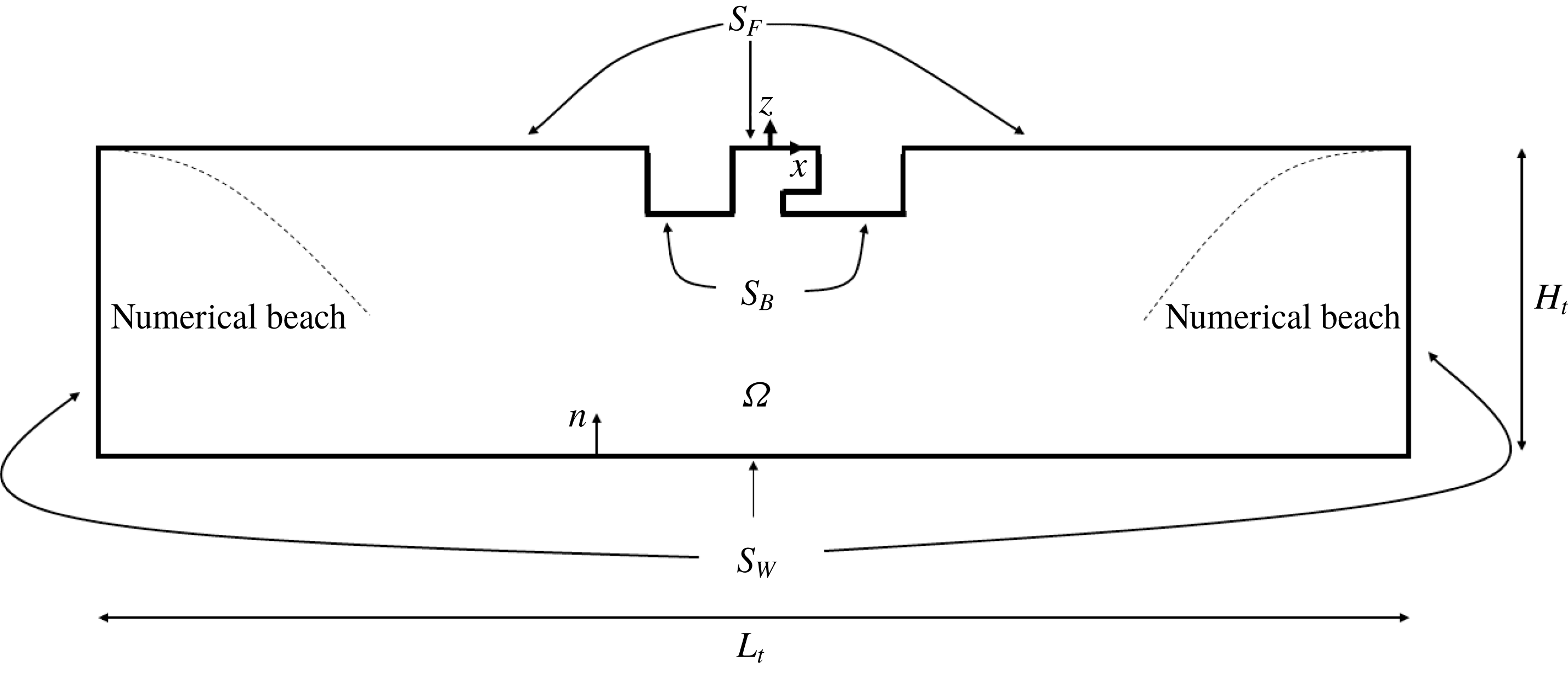
is the time-independent domain of water in the linearized problem (cf. figure 2);
 $\boldsymbol{u}=[u,w]$
is a vector with the horizontal and vertical velocity components. The BEM formulation is widely described in the literature, see e.g. Faltinsen & Timokha (Reference Faltinsen and Timokha2009), and is used in the present BEM to solve for
 $\unicode[STIX]{x1D719}$
. Here we use a distribution of sources and dipoles on the surfaces enclosing the computational domain,
 $$\begin{eqnarray}\unicode[STIX]{x1D6FC}\unicode[STIX]{x1D719}=-\unicode[STIX]{x2A0D}_{S}\unicode[STIX]{x1D719}\frac{\unicode[STIX]{x2202}\unicode[STIX]{x1D713}}{\unicode[STIX]{x2202}n}\,\text{d}S+\int _{S}\unicode[STIX]{x1D713}\frac{\unicode[STIX]{x2202}\unicode[STIX]{x1D719}}{\unicode[STIX]{x2202}n}\,\text{d}S,\end{eqnarray}$$
where
 $S=S_{W}+S_{F}+S_{B}$
(cf. figure 2),
 $\unicode[STIX]{x1D713}=\log r$
,
 $\unicode[STIX]{x1D6FC}=\unicode[STIX]{x03C0}$
on flat elements and
 $\unicode[STIX]{x1D719}$
is the velocity potential which satisfies the Laplace equation,
 $\unicode[STIX]{x1D6FB}^{2}\unicode[STIX]{x1D719}=0$
, in
 $\unicode[STIX]{x1D6FA}$
. The first term on the right-hand side in (3.1) is a principal value integral, due to the singularity located at the collocation point. A lowest-order method is applied, i.e. the source and dipole strengths are constant over each panel.
Conceptual sketch of numerical wave tank for BEM simulations. Numerical beaches are indicated by dashed lines, but are not a part of the mesh itself.
 $L_{t}$
and
 $H_{t}$
are the length and height of the numerical wave tank.
 $H_{t}=1.0~\text{m}$
is used in the present simulation, consistent with the present experiments (cf. § 4).

The presently implemented BEM code has been verified against linear wave-maker theory, see e.g. Dean & Dalrymple (Reference Dean and Dalrymple1991). Discrepancies of less than 1 % were obtained for the wave amplitude using meshes similar to those used in the present study.
The mesh consists of 80 elements per wavelength, i.e. a dedicated mesh is created for each period. A total of approximately 1800 panels is used for the meshes in the present study. The time step is
 $\unicode[STIX]{x0394}t=T/100$
(where
 $T$
is the period), and each simulation is run for approximately 60 oscillations (around the first sloshing mode, approximately 200 periods are needed, as discussed in § 5.3.1). The CPU time is approximately 45 s on a single 3.6 GHz CPU for a simulation with 60 oscillations. Numerical beaches are implemented at the ends of the tank, to avoid reflected waves, by introducing artificial dissipation in the kinematic and dynamic free-surface conditions,
 $$\begin{eqnarray}\displaystyle & \displaystyle \frac{\unicode[STIX]{x2202}\unicode[STIX]{x1D701}}{\unicode[STIX]{x2202}t}=\frac{\unicode[STIX]{x2202}\unicode[STIX]{x1D719}}{\unicode[STIX]{x2202}z}-\unicode[STIX]{x1D708}_{1}(x)\unicode[STIX]{x1D701},\quad \text{on }S_{F}, & \displaystyle\end{eqnarray}$$
 $$\begin{eqnarray}\displaystyle & \displaystyle \frac{\unicode[STIX]{x2202}\unicode[STIX]{x1D719}}{\unicode[STIX]{x2202}t}=-g\unicode[STIX]{x1D701}-\unicode[STIX]{x1D708}_{2}(x)\unicode[STIX]{x1D719},\quad \text{on }S_{F}, & \displaystyle\end{eqnarray}$$
 $\unicode[STIX]{x1D708}_{1}(x)$
and
 $\unicode[STIX]{x1D708}_{2}(x)$
are third-order polynomials in the longitudinal direction, and their magnitudes are empirically determined to be
 $\unicode[STIX]{x1D708}_{1}(\pm L_{t}/2)=0.85~\text{s}^{-1}$
and
 $\unicode[STIX]{x1D708}_{2}(\pm L_{t}/2)=0.47~\text{s}^{-1}$
;
 $L_{t}$
is the length of the numerical tank. The length of the numerical tank is varied such that there are eight wavelengths (
 $8\unicode[STIX]{x1D706}$
, where
 $\unicode[STIX]{x1D706}$
is the wavelength) on each side of the oscillating body. Experience shows that the numerical beach should be at least
 $2\unicode[STIX]{x1D706}-3\unicode[STIX]{x1D706}$
long. The solution is time stepped using an explicit fourth-order Runge–Kutta scheme for the kinematic and dynamic free-surface conditions ((3.2a
) and (3.2b
)).
3.2 Navier–Stokes solver
A Navier–Stokes solver is implemented in order to capture viscous effects related to flow separation, and this method will be referred to as CFD. The present hybrid method is based on previous work by Kristiansen & Faltinsen (Reference Kristiansen and Faltinsen2012), but differs slightly by the fact that the inviscid domain is only the uppermost cell layer in the present CFD. Incompressible Newtonian fluid properties are assumed. The flow is solved using the finite volume method (FVM). The governing equations are solved with linear body-boundary conditions on the oscillating body, and linear free-surface conditions at
 $z=0$
. The governing equations and the assumptions in the present method will be described in the remainder of this section.
The momentum equation,
 $$\begin{eqnarray}\unicode[STIX]{x1D70C}\frac{\unicode[STIX]{x2202}\boldsymbol{u}}{\unicode[STIX]{x2202}t}+\unicode[STIX]{x1D70C}\boldsymbol{u}\boldsymbol{\cdot }\unicode[STIX]{x1D735}\boldsymbol{u}=-\unicode[STIX]{x1D735}p+\unicode[STIX]{x1D707}\unicode[STIX]{x1D6FB}^{2}\boldsymbol{u}+\unicode[STIX]{x1D705}(x)\boldsymbol{u},\end{eqnarray}$$
is solved in the viscous domain, whereas the advection and diffusion terms are neglected in the potential flow domain. Here,
 $\boldsymbol{u}=[u,w]$
and
 $p$
are velocities in the
 $x$
- and
 $z$
-directions, and pressure in the computational domain, respectively. Numerical beaches are modelled by introducing a source term proportional to the velocity (
 $\unicode[STIX]{x1D705}(x)\boldsymbol{u}$
) in the Navier–Stokes equations;
 $\unicode[STIX]{x1D705}(x)$
is a third-order polynomial, with a magnitude such that
 $\unicode[STIX]{x1D705}(\pm L_{t}/2)/\unicode[STIX]{x1D70C}=1.0~\text{s}^{-1}$
at the tank ends (the tank and beach lengths are discussed in § 3.3);
 $\unicode[STIX]{x1D707}$
and
 $\unicode[STIX]{x1D70C}$
are the dynamic viscosity and density of water, respectively. The governing equations are constituted by the momentum equation (3.3) and the continuity equation
 $$\begin{eqnarray}\frac{\unicode[STIX]{x2202}u}{\unicode[STIX]{x2202}x}+\frac{\unicode[STIX]{x2202}w}{\unicode[STIX]{x2202}z}=0.\end{eqnarray}$$
The Navier–Stokes equations are solved using Chorin’s projection method. This implies solving for an intermediate velocity field in an intermediate substep *. The velocity field in substep * is not, in general, divergence free. Consequently, a Poisson equation for the pressure is obtained as
 $$\begin{eqnarray}\unicode[STIX]{x1D6FB}^{2}p^{n+1}=\frac{1}{\unicode[STIX]{x0394}t}\unicode[STIX]{x1D735}\boldsymbol{\cdot }\boldsymbol{u}^{\ast }.\end{eqnarray}$$
Given
 $p^{n+1}$
, a divergence-free velocity field,
 $\boldsymbol{u}^{n+1}$
, is obtained, where
 $n$
is the time step. The Navier–Stokes equations are time marched using an explicit fourth-order Runge–Kutta scheme. The time step,
 $\unicode[STIX]{x0394}t$
, is varied between
 $\unicode[STIX]{x0394}t=T/60$
and
 $\unicode[STIX]{x0394}t=T/120$
depending on the forced heave amplitude,
 $\unicode[STIX]{x1D702}_{3a}$
, and period,
 $T$
. The CPU time is between 105 and 125 min for a simulation with 60 oscillations and
 $\unicode[STIX]{x0394}t=T/80$
on a single 3.6 GHz CPU.
The present CFD solves the laminar problem. In reality, flows with separated vortical structures (wake flows) quickly become turbulent. As discussed in Kristiansen & Faltinsen (Reference Kristiansen and Faltinsen2008), the primary vortices were shown to provide the main contribution to damping of the moonpool response. Since the vortices travelled away from the moonpool in pairs, a turbulence model was found not to be necessary. A difference in the present study is additional vortical structures from the top recess corner, which may or may not remain in the moonpool over a period of oscillation, and this is briefly discussed in § 5.
3.2.1 Boundary conditions
Along the solid walls at the tank ends and bottom, no-slip conditions are applied. The normal derivative of the pressure is set to zero on the tank walls. On the oscillating body, linear body-boundary conditions are applied (i.e. the mesh remains undeformed). This implies that velocities are specified at the mean position. Linear boundary conditions on the body surfaces can be justified if the amplitude of the flow is considerably larger than the amplitude of the body motion. The body-boundary condition for the pressure is
 $$\begin{eqnarray}\frac{\unicode[STIX]{x2202}p}{\unicode[STIX]{x2202}n}=-\unicode[STIX]{x1D70C}\boldsymbol{a}\boldsymbol{\cdot }\boldsymbol{n},\end{eqnarray}$$
which is derived from the Navier–Stokes equations, neglecting the nonlinear and viscous terms. Here,
 $\boldsymbol{a}=[a_{x},a_{z}]$
is the acceleration of the body in the
 $x$
- and
 $z$
-directions, and
 $\boldsymbol{n}$
is the normal vector pointing into the water.
Linearized free-surface conditions are applied at
 $z=0$
. The free-surface elevation,
 $\unicode[STIX]{x1D701}$
, is evolved in time according to the kinematic boundary condition
 $$\begin{eqnarray}\frac{\unicode[STIX]{x2202}\unicode[STIX]{x1D701}}{\unicode[STIX]{x2202}t}=w|_{z=0}.\end{eqnarray}$$
The dynamic boundary condition for the linear pressure on
 $z=0$
is
 $$\begin{eqnarray}p=\unicode[STIX]{x1D70C}g\unicode[STIX]{x1D701}.\end{eqnarray}$$
The present hybrid solver assumes that viscous effects are negligible close to the free surface.
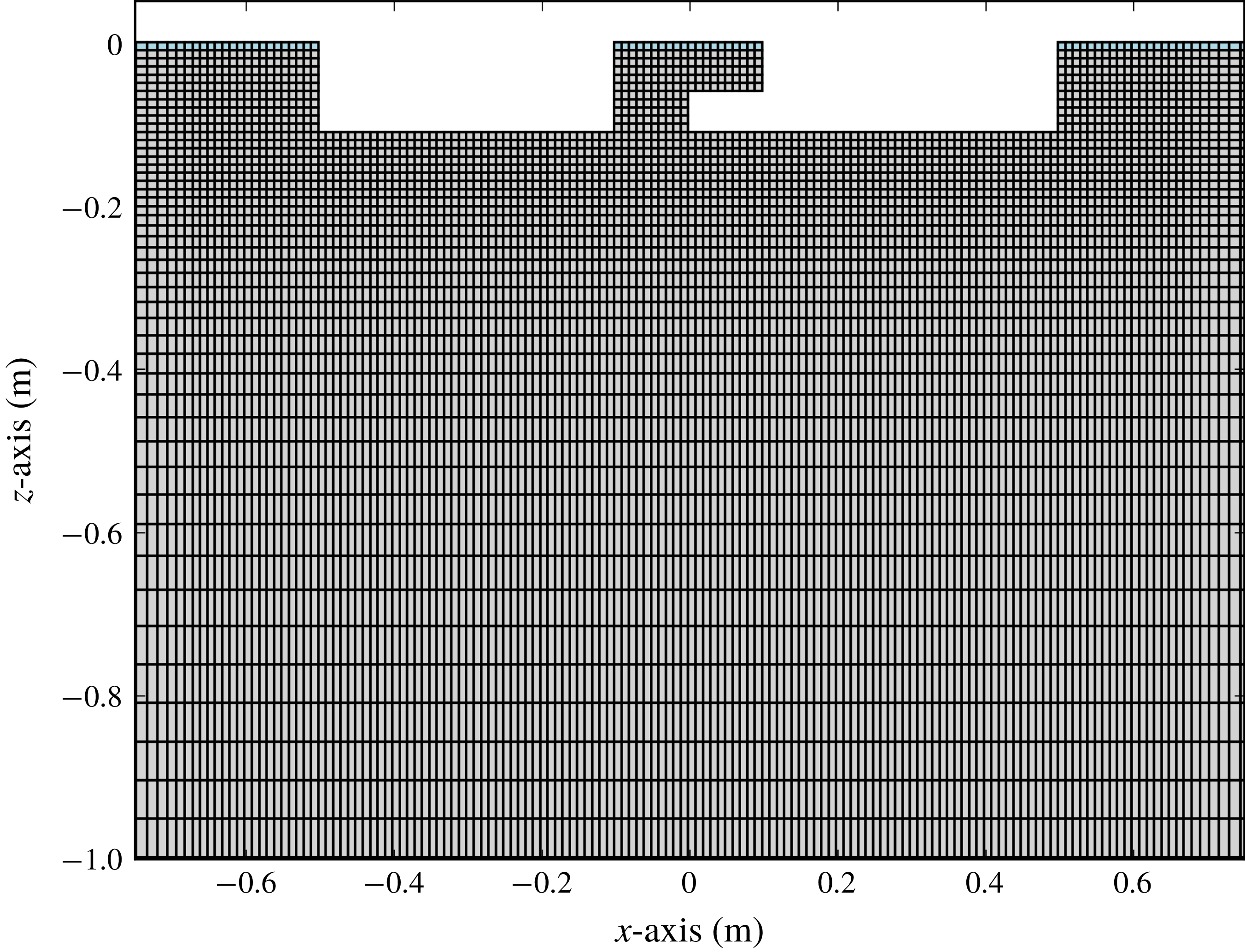
An example of mesh for the presently developed hybrid CFD for Case 3. The uppermost cell layer constitutes the linear potential flow theory domain, while the remaining cells constitute the viscous domain. The figure is zoomed in around the structure. Mesh stretching is applied from
 $x=\pm 0.7~\text{m}$
and
 $z=-0.2~\text{m}$
.

3.3 CFD mesh
Figure 3 shows an example of a discretized fluid domain. The present CFD simulations are performed for the moonpool geometries described in § 4. Across the moonpool the grid consists of 20 cells, while 40 cells are used along the bottom of each box. This corresponds to a mesh size of
 $\text{d}x=\text{d}z=0.01~\text{m}$
in the finest region. Stretching of the cell size is applied from
 $x=\pm 1.0~\text{m}$
and
 $z=-0.3~\text{m}$
. The mesh is stretched with a factor of 1.07 per cell, until a maximum limit of
 $\text{d}x_{max}$
or
 $\text{d}z_{max}$
is reached in the
 $x$
- and
 $z$
-directions, respectively, beyond which the cell size is constant equal to the maximum value; a minimum of 12 cells per wavelength is applied. This mesh density does not solve the details of the boundary layer, since it is assumed that viscous stresses in the boundary layer are of secondary importance, while flow separation from the sharp corners the primary. The length of the tank is varied for each period, with a prescribed length of four wavelengths on each side of the body.
It is found by a dedicated numerical study that a numerical beach with one wavelength is sufficient on each side. On contrary to the numerical beach in the BEM, the present beach dissipates energy more efficiently since the whole water column contributes, while in BEM, naturally, only the elements on the free surface contribute.
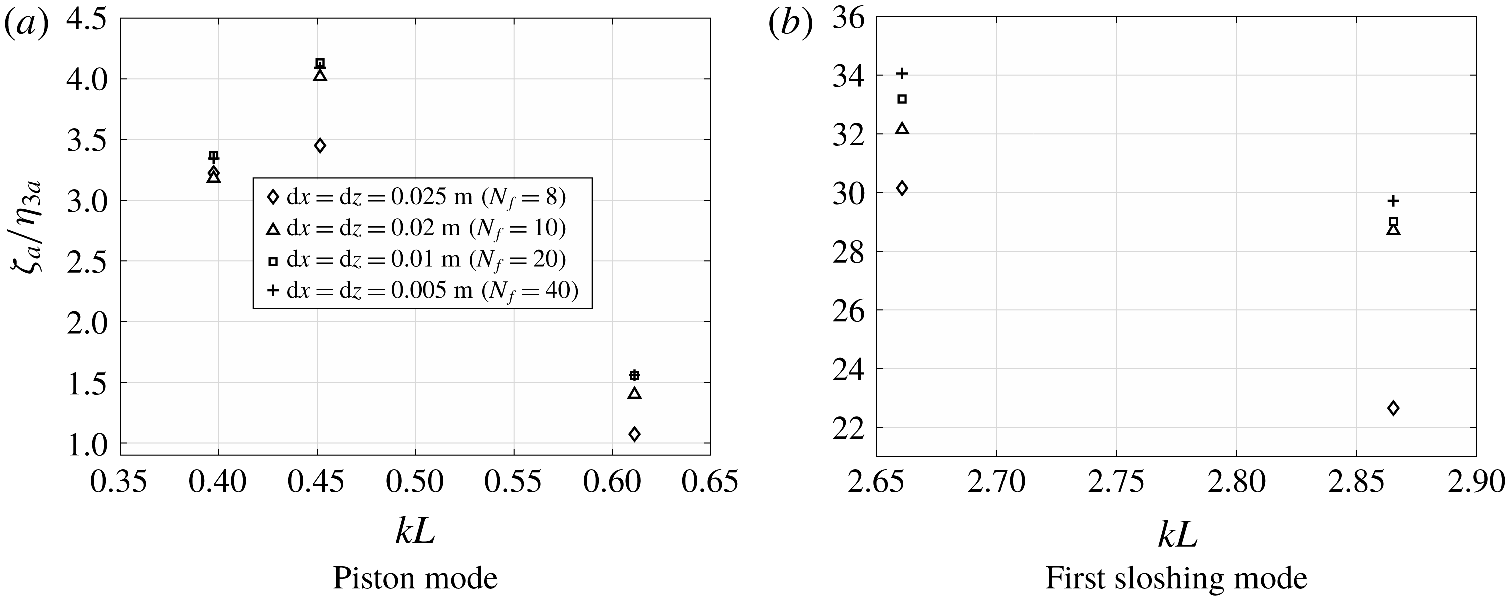
Mesh sensitivity analyses of the present CFD code are presented in figure 4 for Case 3, where the first harmonic response at WP1 for the various mesh sizes is presented. The response is made non-dimensional with respect to the first harmonic heave amplitude,
 $\unicode[STIX]{x1D702}_{3a}$
. Satisfactory convergence is obtained around the piston mode with a difference less than 0.5 % between the finest and presently adopted meshes, which is that with twenty cells across the moonpool, i.e.
 $N_{f}=L/\text{d}x=20$
, where
 $L$
is the length of the moonpool at the mean waterline. Around the first sloshing mode, this difference is less than 2.5 %. The coarsest mesh, with
 $N_{f}=8$
, deviates from the other meshes in general. We found similar results for the three other cases in the present study (not presented).
Kristiansen & Faltinsen (Reference Kristiansen and Faltinsen2012) performed sensitivity analyses on the effect of increasing the potential flow domain over several cell layers. They found that increasing the thickness of the potential flow domain had negligible effect on the responses, as long as the vortical structures of significance were not advected into the potential flow domain. From investigations of the flow predicted by the CFD in the present cases, we did not observe vortical structures wandering into the potential flow domain.
Mesh sensitivity analyses with different mesh sizes for Case 3 at WP1 for selected frequencies. The first harmonic responses are made non-dimensional with respect to
 $\unicode[STIX]{x1D702}_{3a}$
, and
 $\unicode[STIX]{x1D702}_{3a}=1~\text{mm}$
. The finest mesh size, i.e.
 $\text{d}x=\text{d}z=0.005~\text{m}$
indicates that satisfactory convergence is obtained (
 $\text{d}x=\text{d}z=0.01~\text{m}$
was used throughout the study).
 $N_{f}=L/\text{d}x$
is the number of cells over the length of the moonpool at the waterline.

4 Experimental set-up
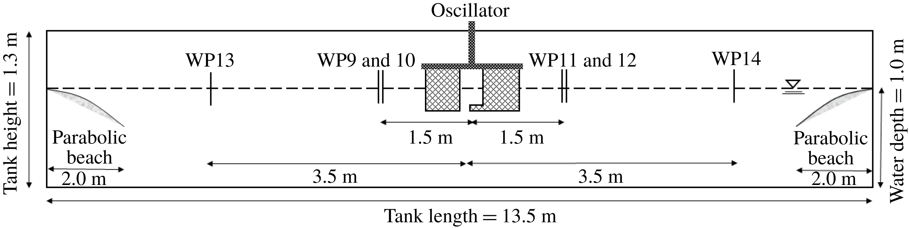
The experiments were carried out in a glass walled wave flume at the Marine Technology Centre in Trondheim. The tank is 13.5 m long and 0.6 m wide. The water depth was 1.0 m during the experiments. Two boxes, each of 40 cm length and 59 cm width, were used to represent the moonpool configuration. Approximately 20 moonpool configurations with recess were tested. Three representative configurations are included here, referred to as Cases 1–3 (see table 1), where the recess length is varied. The distance between the boxes at the mean waterline,
 $L$
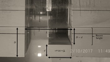
, was chosen to be 20 cm (cf. figure 5). A photo of the set-up for Case 3 is shown in figure 5, which is the set-up with the largest recess included in the present study.
Physical dimensions of the three test cases in the present experiments (cf. figure 5). The natural wavenumber of the transverse sloshing mode is presented as
 $k_{T}L$
, where
 $k_{T}$
is the wavenumber and
 $L$
is the length of the moonpool at the mean waterline.

The experimental tests presented in the present study are a continuation of the ones presented in Ravinthrakumar, Kristiansen & Ommani (Reference Ravinthrakumar, Kristiansen and Ommani2018), where the focus was on empirical modelling of damping of the piston mode in the BEM. In the present study, we include also the first sloshing mode.
The model was forced to heave sinusoidally with varying amplitudes,
 $\unicode[STIX]{x1D702}_{3a}$
, and periods,
 $T$
, as
 $\unicode[STIX]{x1D702}_{3}=\unicode[STIX]{x1D702}_{3a}\sin \unicode[STIX]{x1D714}t$
, where
 $\unicode[STIX]{x1D714}=2\unicode[STIX]{x03C0}/T$
. The heave amplitude was varied between 1 and 5 mm, with a step of 1 mm. The model tests were automated in the sense that a long time series (typically 24 h) was given as input to the oscillator. The time series consisted of a range of sinusoidal signals with varying oscillation amplitudes and periods, in addition to rest times of two minutes for the free surface in the tank to come to rest. Free-surface elevation was measured during the rest time of two minutes. After two minutes the motion was less than 1 % relative to the free-surface elevation amplitude in and outside the moonpool when the model was forced to heave. Typically, 400–500 tests were achieved in a 24 h duration run. Each test consisted of 60 oscillations, which includes five linear ramp ups and ramp downs at the beginning and end of each test.
The free-surface elevation,
 $\unicode[STIX]{x1D701}$
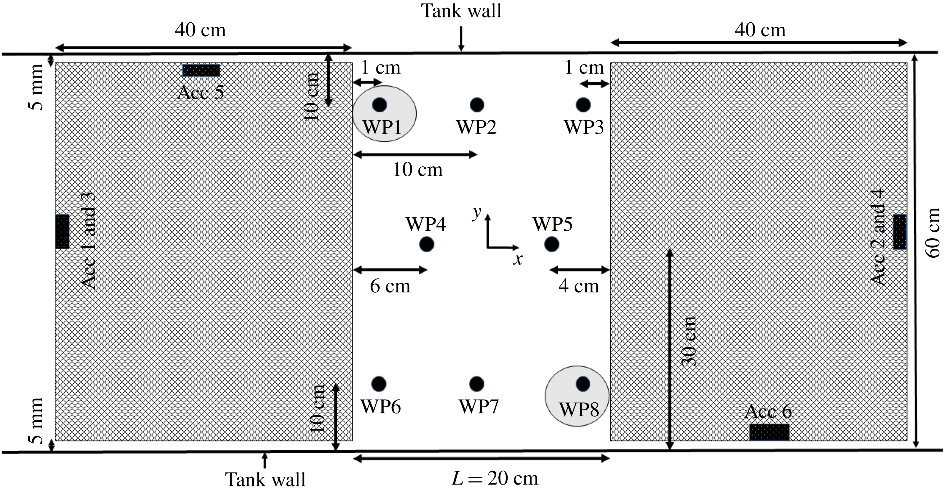
, was measured at eight locations in the moonpool. In addition, six wave probes outside the model (cf. figure 6) were used to check for evidence of reflected waves from the tank ends. Accelerations in the
 $x$
-,
 $y$
- and
 $z$
-directions were measured with six accelerometers (cf. figure 7). The latter to obtain vertical position by integrating twice in time using a standard Fourier transform-based integration method, and the two former to check for possible, unwanted lateral rig oscillations. Forces in the
 $x$
- and
 $z$
-directions were measured, but they are not presented in the present study.
Photo of the experimental set-up in the wave flume at the Marine Technology Centre in Trondheim. Recess floor dimension
 $10~\text{cm}\times 5~\text{cm}$
, draft
 $D=11~\text{cm}$
, moonpool length
 $L=20~\text{cm}$
(Case 3, cf. table 1). Recess height is defined as
 $D-d$
.

Side view of the experimental set-up. The location of the parabolic beaches and wave probes outside the moonpool are indicated.

Bird’s eye view of the set-up, showing the wave probe (WP) locations in the moonpool, and accelerometer (Acc) locations. Results from measurements at WP1 and WP8 are presented in § 5.

4.1 Error analysis in model tests
The model tests were conducted carefully in order to minimize inaccuracies and errors in the measurements. However, possible bias and random errors are addressed to discuss the quality of the experimental results.
4.1.1 Parabolic beaches
The tank is equipped with two parabolic beaches; one on each end of the tank to avoid wave reflection. The parabolic beaches were adjusted prior to each test such that the uppermost point of the beaches was located approximately 2 mm below the free surface, which was found in Kristiansen & Faltinsen (Reference Kristiansen and Faltinsen2012) to be efficient for waves with small wave steepness.
4.1.2 Wave probes
The currently used wave probes are designed to account for temperature variations. The temperature variations in the wave flume were small during the testing period (within
 $1^{\circ }\text{C}$
between each time the wave probes were calibrated). Still a drift in the zero value was observed. This offset was accounted for by daily zero setting, and during post-processing. The paired wave probes gave similar results except when transverse sloshing occurred.
4.1.3 Transverse sloshing and seiching
The first transverse sloshing mode of the wave flume is
 $kL=\unicode[STIX]{x03C0}L/B=1.04$
, but this is affected due to the presence of the recess;
 $k=2\unicode[STIX]{x03C0}/\unicode[STIX]{x1D706}$
and
 $L$
are the wavenumber and length of moonpool at the mean waterline, respectively. The second and third sloshing modes are
 $kL=2.09$
and
 $kL=3.14$
, respectively. Both video recordings and wave elevation measurements were used to detect results containing transverse sloshing. The first sloshing mode in the moonpool for the present cases is in the range
 $2.6<kL<3.1$
, and the piston mode is in the range
 $0.51<kL<0.59$
. The first transverse sloshing mode was excited at narrow ranges in the range
 $1.17<kL<1.39$
, depending on the recess length (cf. table 1). This is between the range of piston and first sloshing mode frequencies, and thus the first transverse sloshing did not affect our presented results. We observed that when the model was forced to heave at the first transverse sloshing mode frequency, transverse sloshing occurred instantly, rather than gradually over time. The second and third transverse modes were not observed to be excited in the first sloshing mode range.
4.1.4 Distance between glass walls and model
A distance of 5 mm was kept between the model and the glass walls of the tank, in order to avoid contact. This introduces a 3-D effect. This gap is, however, not more than 1.67 % of the total width of the tank, so the mass flux of water in and out of the gap between the glass wall and the model is small, although it represents a source of error. A quantitative analysis of this error was not performed. Similar studies earlier concluded this error was small (see e.g. Kristiansen & Faltinsen (Reference Kristiansen and Faltinsen2012)).
4.1.5 Repeatability
Selected periods with Case 3 were repeated eight times for forced heave amplitudes
 $\unicode[STIX]{x1D702}_{3a}=1~\text{mm}$
, 3 mm and 5 mm. The response amplitude operators (RAOs) and time series correspond well; in the piston mode frequency range (
 $0.4<kL<0.7$
), the largest standard deviation in the RAO is less than 1 %. In the range of the first sloshing mode (
 $2.25<kL<3.4$
), the largest standard deviation in the RAO is less than 2.5 %. The somewhat larger discrepancy around the first sloshing mode is likely to be related to the fact that the free-surface motion is larger, and to some extent nonlinear, in this range of
 $kL$
.
4.1.6 Accelerometers versus position sensor
The vertical motion of the model was measured also with a draw-wire sensor. The accelerometers and the draw-wire sensor were in good agreement: in general, differences less than 1.5 % were observed. On some occasions, however, the displacement sensor failed for unknown reasons. Consequently, the accelerometers are used for determining the heave motion,
 $\unicode[STIX]{x1D702}_{3}$
, in the present study.
Both accelerometers and draw-wire sensor measurements are used to ensure that the prescribed forced heave period was achieved in the experiments.
5 Results and discussion
Amplitude-dependent RAOs from the experiments are presented, along with numerical results. The results are presented separately for the piston and sloshing modes. The RAOs are defined as
 $\unicode[STIX]{x1D701}_{a}/\unicode[STIX]{x1D702}_{3a}$
, where both quantities are amplitudes of the first harmonic of the time series in a steady time window in an Earth-fixed coordinate system. Higher harmonics are very small for all the cases in the present study, except in the proximity of the first sloshing mode (cf. § 5.3). Five oscillation amplitudes are tested, but only three of them are presented in the RAOs for the sake of clarity.
RAOs for the configurations studied in the present study. The RAOs are defined as
 $\unicode[STIX]{x1D701}_{a}/\unicode[STIX]{x1D702}_{3a}$
, where
 $\unicode[STIX]{x1D701}_{a}$
and
 $\unicode[STIX]{x1D702}_{3a}$
are amplitudes of the first harmonic of the time series in a steady time window of the wave gauge and vertical forced motion, respectively. BEM results shown with experimental results for
 $\unicode[STIX]{x1D702}_{3a}=1~\text{mm}$
.

5.1 Natural period predictions and mode shapes
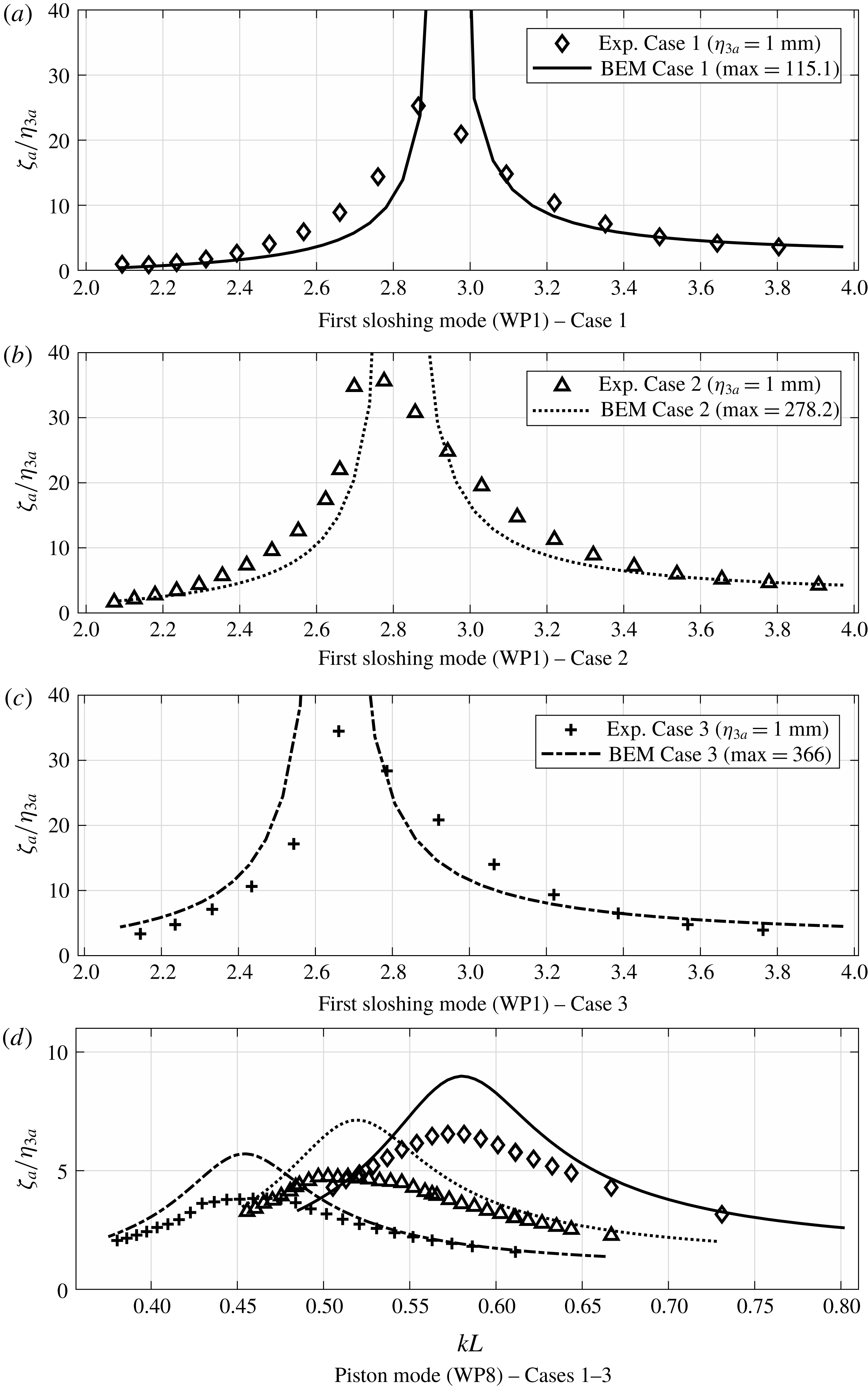
RAOs of both the first sloshing mode (cf. figure 8
a–c) and piston mode (cf. figure 8
d) for
 $\unicode[STIX]{x1D702}_{3a}=1~\text{mm}$
are presented in figure 8 together with numerical results from the BEM. The largest free-surface elevation for the piston mode occurs at the recess wall end. For the first sloshing mode, the largest response occurs at the opposite wall end. Consequently, the RAOs for the piston and sloshing modes are presented at the locations of WP8 and WP1, respectively (cf. figure 7).
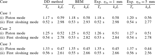
The natural periods calculated from the DD method presented in § 2, along with natural periods from the experiments and predicted with BEM, are presented in table 2. The natural periods from the BEM simulations are found by performing approximately 50 simulations with different periods close to the natural period predicted by the DD method, and choosing that with the maximum response as the natural period. The predicted natural frequencies with the present DD method are in good agreement with BEM, where the difference is 1.8 % at most. Fair agreement is also observed with the experiments, with a slight shift in the natural frequencies for all cases. This is likely to be due to viscous effects in the proximity of the piston mode, and Duffing-type behaviour in the vicinity of the first sloshing mode, as discussed in §§ 5.2 and 5.3.
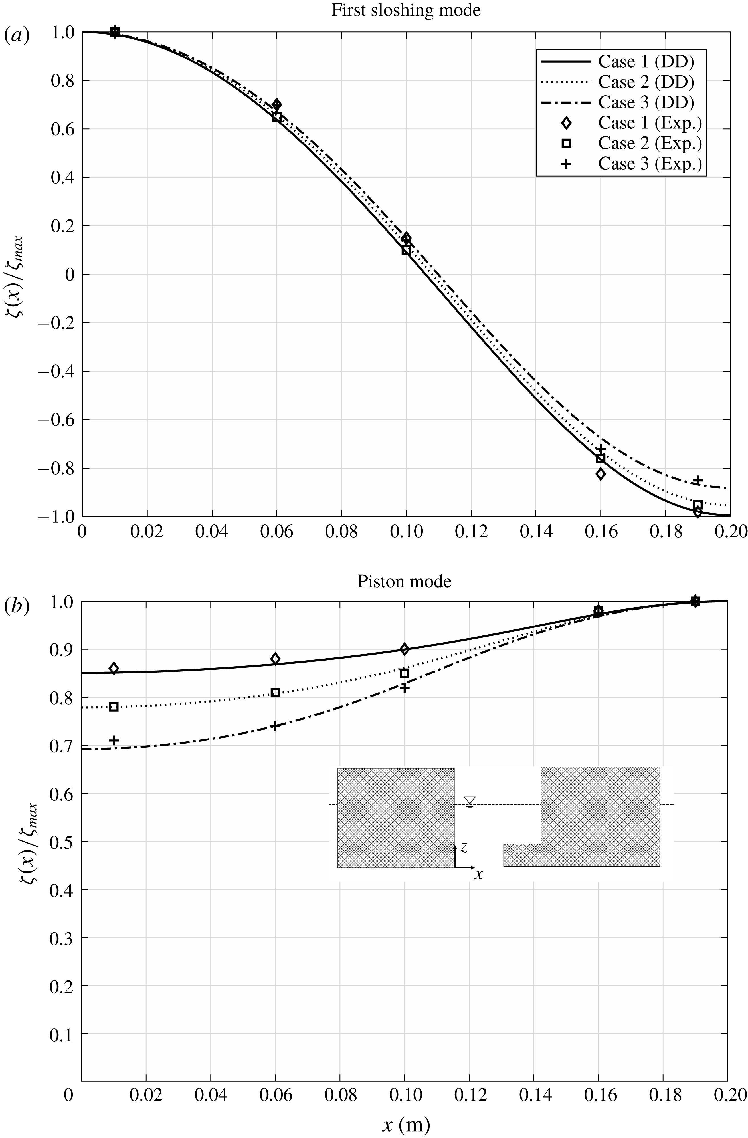
Mode shapes of the piston and first sloshing modes are presented in figure 9. Interestingly, the maximum free-surface elevation,
 $\unicode[STIX]{x1D701}_{max}$
, occurs at the wall over the recess. The variation along the moonpool increases with increasing recess length. This was first observed by Molin (Reference Molin2017). The author found this fact to be a bit surprising, since intuitively, one would expect the opposite due to that the vertical flow through the moonpool inlet would cause larger free-surface elevations there. In this study, no experimental data were presented. The present experimental data leave no doubt about the physical soundness of the phenomenon. The (small) discrepancies between the experimental data and present analytic mode shapes must be interpreted to be within experimental uncertainty.
The mode shape of the first sloshing mode is less affected by the recess for the present configurations. The experimental data support the analytic results also here.
Natural periods,
 $T_{n}$
, and non-dimensional wavenumbers,
 $k_{n}L$
, predicted by present BEM simulations, and DD method (truncated after 25 terms).
 $L$
is the length of the moonpool at the waterline and
 $k_{n}$
is the wavenumber corresponding to
 $T_{n}$
. Experimental results (Exp.) are also shown for two forced heave amplitudes.

Mode shapes predicted by the presently developed DD method (cf. § 2) shown by curves. The largest free-surface elevation occurs at the recess wall end for the piston mode, and the opposite wall end for the first sloshing mode. Experimental results (Exp.) at resonance for the smallest forced heave amplitude,
 $\unicode[STIX]{x1D702}_{3a}=1~\text{mm}$
, are also indicated with the first harmonic response amplitudes made non-dimensional by the maximum first harmonic response amplitude measured in the moonpool. Increasing the recess length has a significant influence on the piston mode shape.

5.2 Amplitude-dependent piston mode RAOs
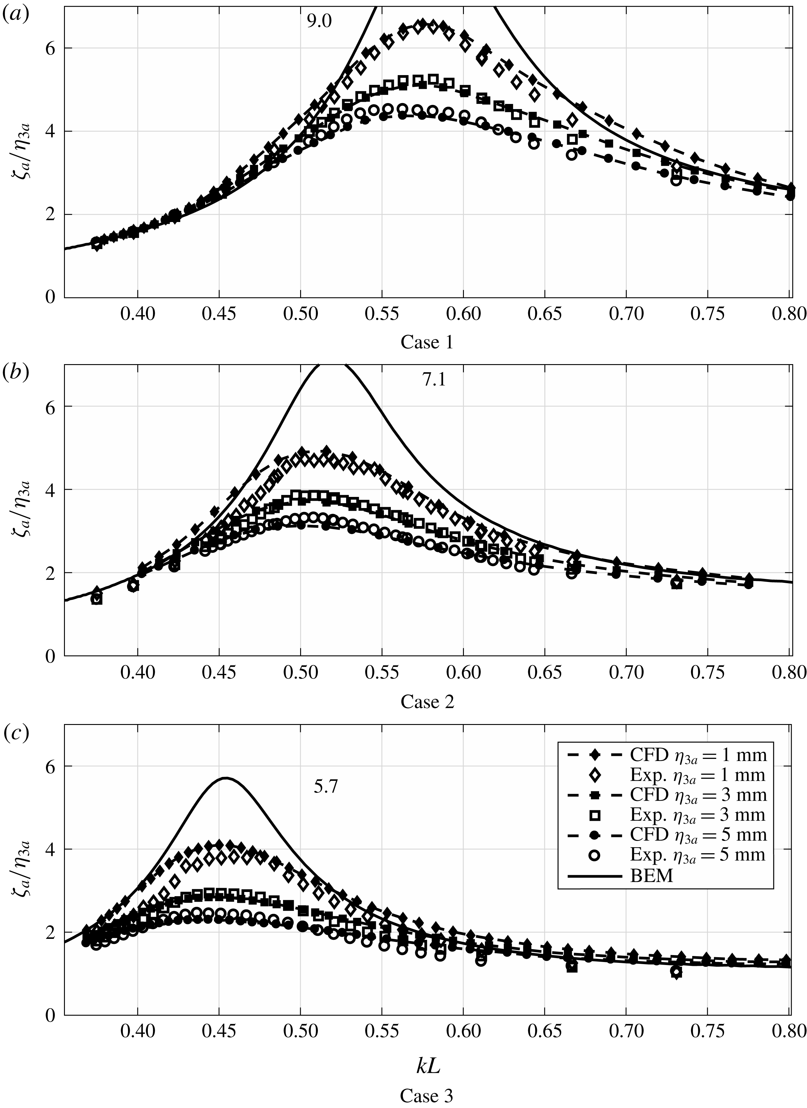
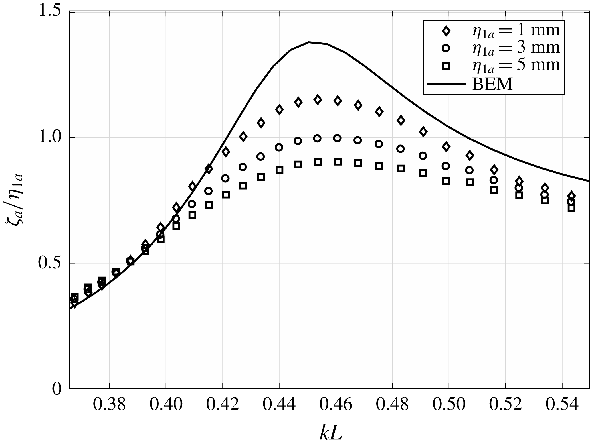
Amplitude-dependent RAOs for Cases 1–3 in a range of periods around the piston mode are presented in figure 10. The results indicate a clear damping contribution due to flow separation at the piston mode resonance, as established for clean moonpools. The BEM results clearly over-predict, since damping due to flow separation is not accounted for. The agreement between the CFD and experimental results is in general fair.
Piston mode RAOs from the present experiments, presently developed hybrid CFD and BEM (WP8). Damping due to flow separation is important at piston mode resonance. The numbers indicate the peak magnitudes at resonance as predicted by BEM.

A slight shift of the resonance peaks is noticed when
 $\unicode[STIX]{x1D702}_{3a}$
increases, most likely due to that flow separation causes amplitude-dependent added mass, in addition to amplitude-dependent damping.
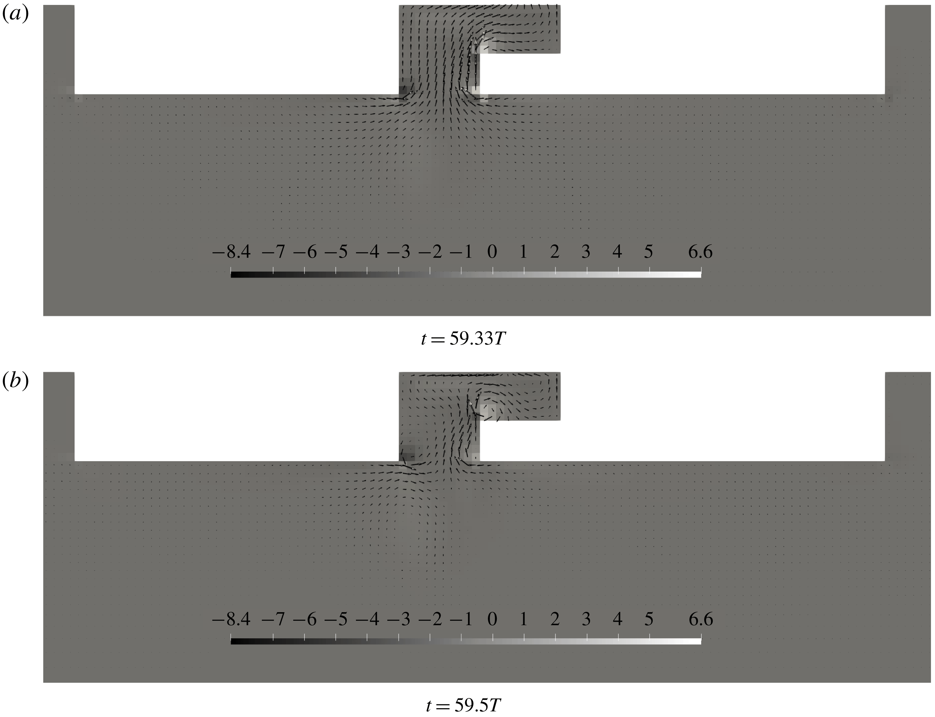
Flow separation both at the moonpool inlets and recess corner provide damping on the moonpool response. Kristiansen & Faltinsen (Reference Kristiansen and Faltinsen2012) studied moonpools with rectangular appendages at the inlet of the moonpool, which may be considered as a symmetric moonpool configuration with small recess floors. They observed increased flow separation strength due to the presence of the appendages. The present study is consistent with their investigations. Flow separation at the recess corner is significant for the present cases. Example velocity fields are presented in figure 11.
The present CFD results indicate some discrepancies for
 $kL>0.6$
in figure 10(c), which cannot be explained by non-converged results (cf. § 3.3). We believe this is related to the linear body-boundary conditions, which prevent full development of detached vortices in this frequency range. The reason is that the relative flow is not dominated by the water motions in this frequency range. This is, as mentioned earlier, important to justify linear body-boundary conditions. Fredriksen et al. (Reference Fredriksen, Kristiansen and Faltinsen2015) discussed this fact for roll motion of a floating body with a similar hybrid code. They concluded that fully nonlinear body-boundary conditions were necessary for roll damping, and that linear body-boundary conditions were inadequate. For the cases with smaller recess lengths, i.e. Cases 1 and 2, the CFD compares better with BEM and experiments outside resonance.
Contour plots of the vorticity (
 $\unicode[STIX]{x1D735}\times \boldsymbol{u}$
) in the flow field for Case 3 at two time instances at the piston mode from the present CFD in forced heave.
 $\boldsymbol{u}$
is indicated with vectors.
 $kL=0.58$
and
 $\unicode[STIX]{x1D702}_{3a}=1~\text{mm}$
.

5.3 First sloshing mode
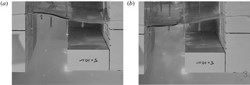
The recess introduces asymmetric flow in the moonpool, meaning that sloshing is induced. Figure 12 shows two photos illustrating the shape of the first sloshing mode in the moonpool for Case 3. Large moonpool motions were observed in the experiments, but no wave breaking was observed for the present cases.
Two consecutive photos, approximately half the sloshing period apart, illustrating the free-surface shape of the first sloshing mode for Case 3 (cf. table 1).
 $\unicode[STIX]{x1D702}_{3a}=1~\text{mm}$
and
 $kL=2.66$
.

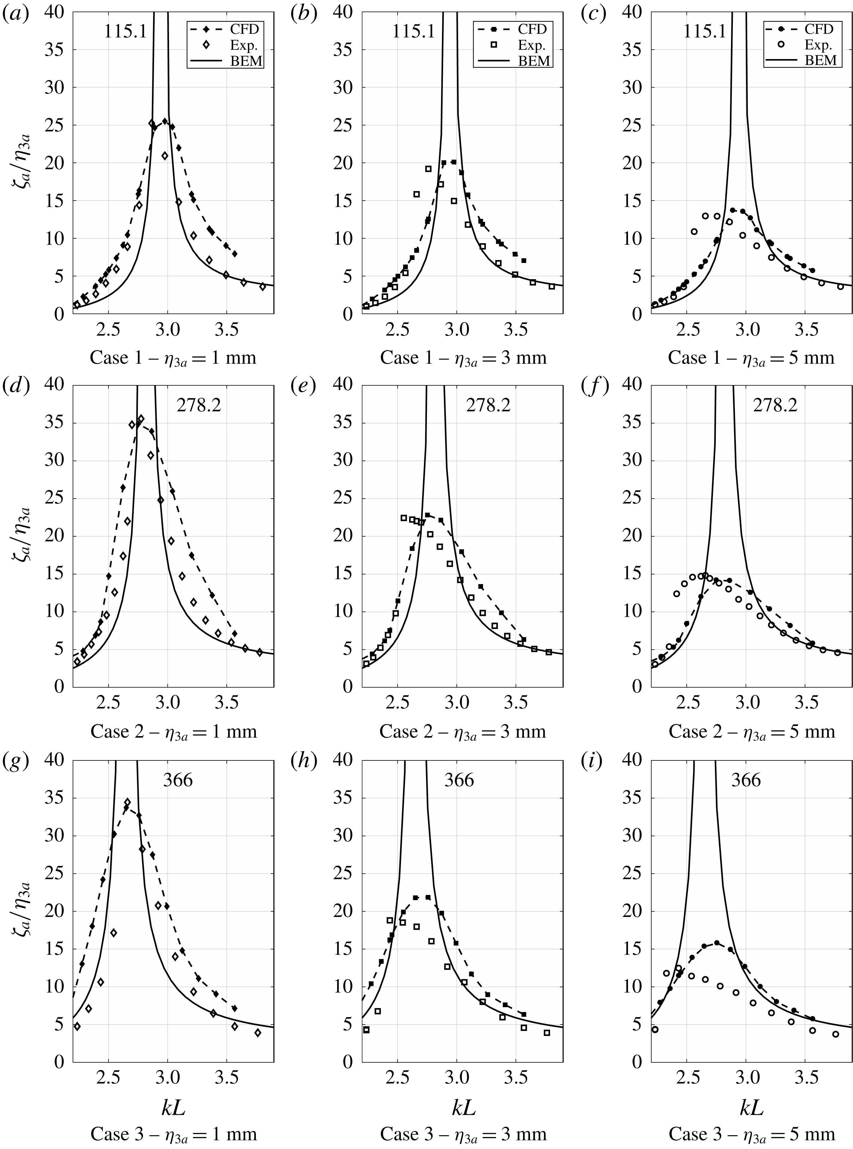
First sloshing mode RAOs from the experiments, presently implemented hybrid CFD and BEM (WP1). Viscous damping is clearly dominant at first sloshing mode. Nonlinear Duffing-type free-surface behaviour is observed in the experimental results. The numbers indicate the peak magnitudes at resonance as predicted by BEM.

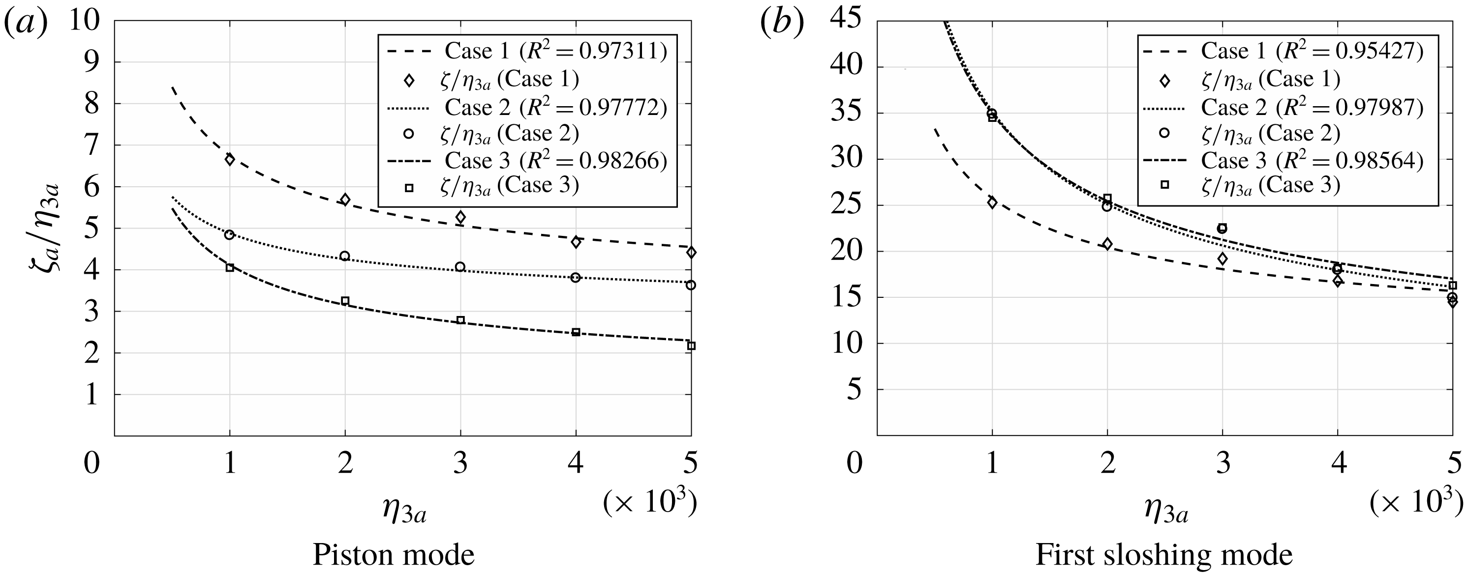
First sloshing mode RAOs at WP1 are presented in figure 13. The measured sloshing RAOs are significant; up to 35 in the tested range. The BEM results significantly over-predict the response at resonance, much more than for the piston mode. The reason is very limited wave radiation caused by the sloshing for the present configurations. The predicted RAO at the sloshing natural frequency predicted by the BEM is approximately 300–400. Evidence of that the damping is quadratic is provided in figure 14. Here the maximum RAOs at resonance are presented as a function of
 $\unicode[STIX]{x1D702}_{3a}$
. With quadratic damping, the maximum responses decrease as
 ${\unicode[STIX]{x1D702}_{3a}}^{-1/2}$
, when presented as
 $\unicode[STIX]{x1D701}_{a}/\unicode[STIX]{x1D702}_{3a}$
.
One of the objectives of the present work was to study the importance of damping due to flow separation in the vicinity of the first sloshing mode. Damping due to flow separation is significant in the proximity of the first sloshing mode, as indicated by the experimental and CFD RAOs. Although viscous effects explain a major part of the discrepancies between experimental and potential flow results, there are clear nonlinear free-surface effects observed in the RAOs for the first sloshing mode. The experimental RAOs for Cases 1–3 indicate that the moonpool response follows a soft Duffing oscillator-like behaviour (cf. figure 13). In order to improve the numerical predictions, nonlinear free-surface effects must be modelled. One alternative to achieve this is to apply a surface capturing technique such as volume of fluid (VOF), as done by Ommani et al. (Reference Ommani, Kristiansen, Berget, Sandvik and Faltinsen2016).
When the water height above the recess is varied, this Duffing-like behaviour is likely to alternate between a soft and hard Duffing oscillator, depending on the draft and recess dimensions. Faltinsen & Timokha (Reference Faltinsen and Timokha2009) show that the response curves change from hard to soft spring behaviour at
 $h/L=0.3368$
for a closed sloshing tank, where
 $h$
is the water depth in the tank. Similar behaviour might be the case for moonpools with a recess, depending on the recess dimensions and the draft. Here,
 $h/L$
is equal to 0.3 in the recess and is nearly infinite in the remaining part of the moonpool. Hence, it makes sense that a soft spring behaviour is observed.
The CFD and experimental RAOs indicate that the nonlinear effects increase with increasing recess length. The Duffing-type responses are clear for all cases. For Cases 1 and 2, the maximum responses in the experimental RAOs are in fair agreement with the maximum responses predicted by CFD for all
 $\unicode[STIX]{x1D702}_{3a}$
. For Case 3, the nonlinear effects are more significant, with a discrepancy of approximately 20 % between the experiments and CFD, where CFD over-predicts.
In the remaining part of the paper, the focus is on identifying the main source of damping in the proximity of the first sloshing mode, acknowledging that Duffing-type nonlinearities are important, especially for large recess lengths, but not dominant in terms of the maximum responses.
Regression of the maximum responses at resonance as predicted by forced heave motion simulations with the present CFD for the five forcing amplitudes studied. Damping at resonance is dominated by viscous effects, mainly quadratic with the relative motion between the flow and body motions. The maximum responses are fitted to a curve of the form
 $\unicode[STIX]{x1D701}_{a}/\unicode[STIX]{x1D702}_{3a}=c_{0}+a_{0}{\unicode[STIX]{x1D702}_{3a}}^{-1/2}$
.

5.3.1 Beating close to first sloshing mode
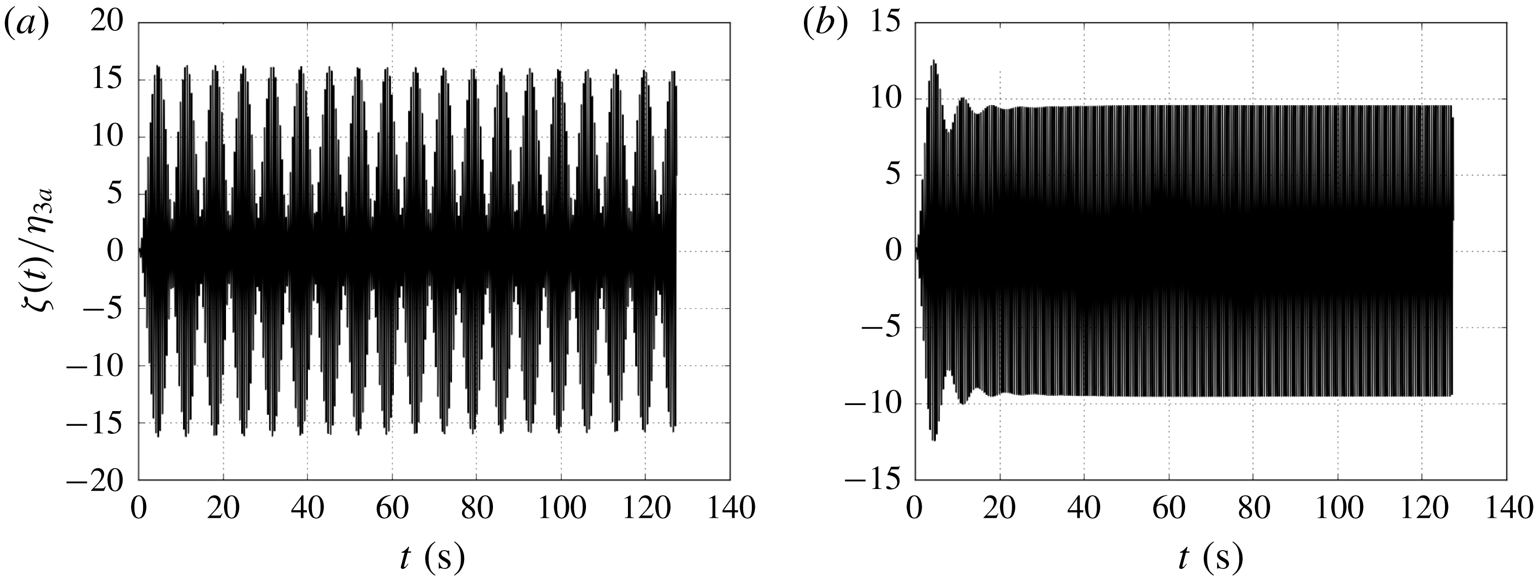
Around the first sloshing mode, radiation damping is considerably smaller than for the piston mode, due to significantly lower flux through the moonpool entrance. In the proximity of the first sloshing mode, beating might occur in the moonpool response (cf. figure 15). In the present BEM simulations, artificial damping is applied and linearly released to shorten the transients. The artificial damping is applied uniformly on the free surface in the moonpool, and released after 100 oscillations.
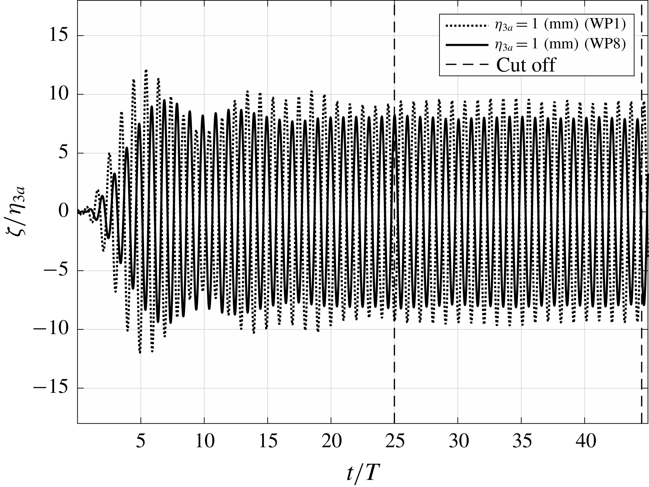
Beating is also present in the CFD and the experiments, although much less pronounced than in the BEM. An example time series for the lowest forcing amplitude is shown in figure 16 for Case 2 with
 $\unicode[STIX]{x1D702}_{3a}=1~\text{mm}$
. The transient is damped out after 25 oscillations. At forcing amplitudes higher than 1 mm the beating is considerably less pronounced.
Free-surface elevation at WP1 for Case 3, predicted by BEM under forced harmonic motion close to the first sloshing mode (
 $kL=3.1$
). Artificial damping is needed to achieve steady-state results, and is released after
 $t/T=100$
. (a) No artificial damping is applied on the free-surface in the moonpool. The beating maintains for a significant amount of time. (b) Artificial damping is applied to damp out transient beating and obtain steady-state results.

Free-surface elevation for the most pronounced beating observed in the experiments. The steady free-surface oscillations are extracted from the time window indicated by the dashed vertical lines. Experimental results for Case 3, where
 $kL=3.2$
and
 $\unicode[STIX]{x1D702}_{3a}=1~\text{mm}$
.

5.4 Forced surge
The experimental set-up does not permit us to perform forced surge oscillations. In the present work, we investigate the moonpool responses in forced surge conditions numerically, where the model is forced to oscillate as
 $\unicode[STIX]{x1D702}_{1}=\unicode[STIX]{x1D702}_{1a}\sin \unicode[STIX]{x1D714}t$
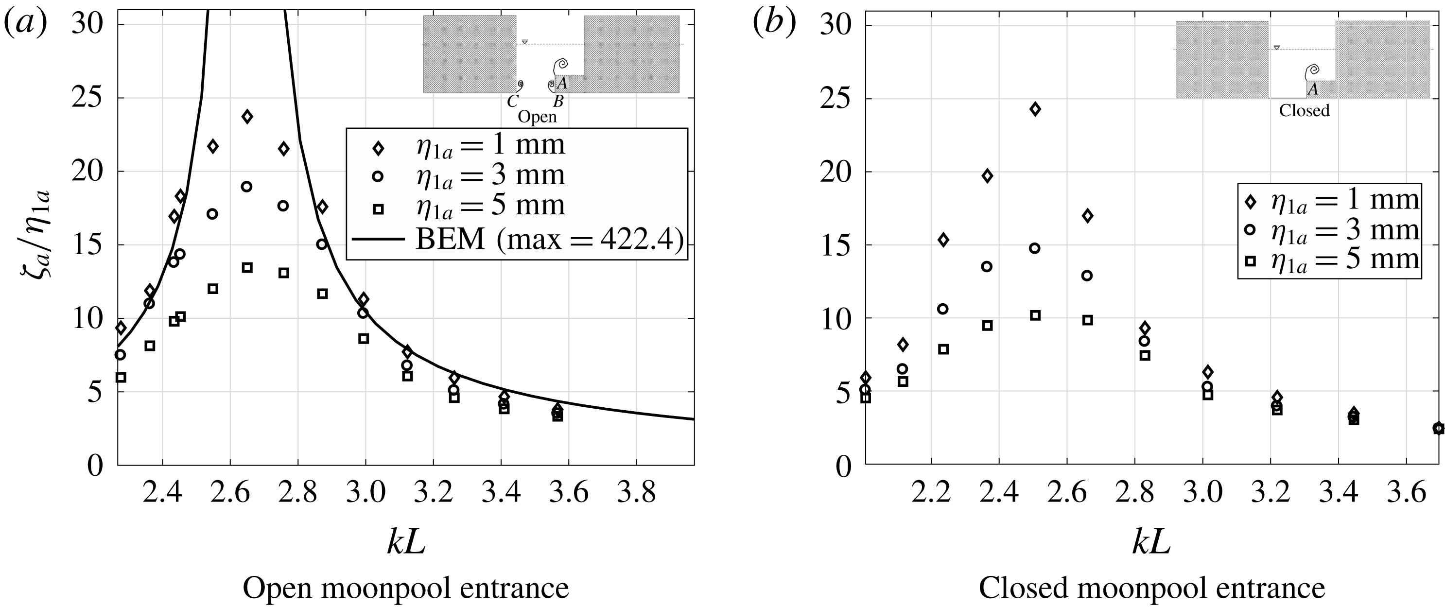
. These studies are performed using the CFD and BEM codes. First sloshing mode RAOs for Case 3 are presented in figure 17(a). As for forced heave, the results show that radiation damping is negligible, and that viscous damping related to flow separation from sharp corners at the recess corner, and possibly at the inlet, is dominant at resonance (similar results are observed for Cases 1 and 2).
As discussed above, the experimental results in forced heave around the natural frequency of the first sloshing mode clearly indicate that nonlinear free-surface effects are important, which is not captured by the present CFD. However, CFD does provide major improvement to the BEM results, which suggests that damping due to flow separation is dominant. The present study is carried out to investigate the dominant effect providing damping on the moonpool motion around the first sloshing mode.
The RAOs are significant. If a model scale of 1:100 is assumed, a surge amplitude of 10 cm of the ship will result in approximately 2.5 m sloshing amplitude. A smaller surge amplitude will result in a correspondingly larger relative sloshing amplitude due to that the damping is mainly quadratic.
Amplitude-dependent first sloshing mode RAOs as predicted by the present CFD for Case 3 with forced surge motions (WP1), with open and closed moonpool entrance. Viscous damping due to flow separation at the sharp corner at point
 $A$
is dominant at the first sloshing mode. Flow separation at points
 $B$
and
 $C$
are of secondary importance due to small flux through the moonpool entrance.

Piston mode RAOs predicted by present CFD and BEM for Case 3 with forced surge motions (WP8).

In order to study the main contribution to the damping of the first sloshing mode in surge, numerical simulations with the CFD solver were performed with closed inlet of the moonpool (i.e. a closed tank with recess), subjected to forced surge motions. The results are provided in figure 17(b). The responses are very similar to those for the cases with open inlet. A small shift in the natural frequency occurs. The similarities in the maximum responses demonstrates the importance of flow separation at the recess corner at the first sloshing mode. We conclude from this that flow separation from the moonpool inlet (points
 $B$
and
 $C$
in figure 17) is of secondary importance under forced surge conditions. We believe this is because the flow through the moonpool entrance is small compared to the flow velocity around the recess corner.
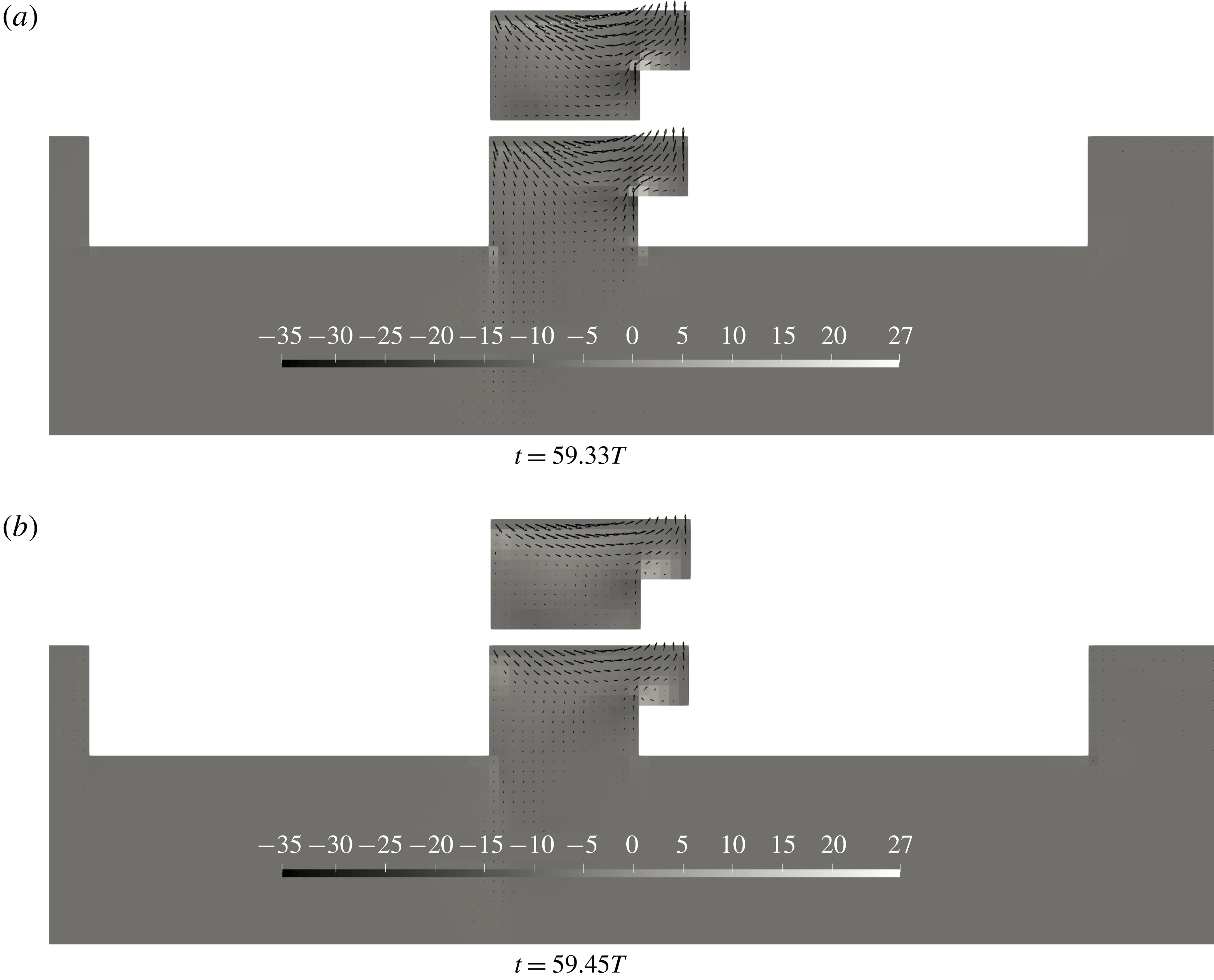
Figure 19 exemplifies the similarities in the flow separation at the top recess corner with both an open and closed inlet for Case 1. Vortices are created due to flow separation at the recess corner, which acts as damping on the sloshing motion in the moonpool and the sloshing tank. Flow separation at the moonpool inlets can be noticed in figure 19, which is significantly smaller than the vorticity at the recess corner, and is of secondary importance for the present cases. For moonpools with larger moonpool lengths, the effect of flow separation at the moonpool inlets is likely to be more prominent, since the flow will reach deeper than for the present cases. Similarly, for larger recess heights, the relative importance of flow separation at the recess corner will become less significant, since the recess corner will be closer to the moonpool inlets.
Figure 18 shows the amplitude-dependent RAO for Case 3 around the piston mode. Due to the asymmetry in the configuration, the piston mode is excited in forced surge conditions. The RAOs show that the piston mode response is significantly lower than for forced heave conditions. Despite very small responses, clear damping effects are introduced by flow separation at the inlets and recess corner.
Contour plots of the vorticity (
 $\unicode[STIX]{x1D735}\times \boldsymbol{u}$
) in the flow field for Case 1 in forced surge at two time instances at the first sloshing mode from the present CFD.
 $\boldsymbol{u}$
is indicated with vectors. Contour plots for the sloshing tank with recess is shown above the moonpool configuration at the same time instance.
 $kL=2.98$
and
 $\unicode[STIX]{x1D702}_{1a}=1~\text{mm}$
.

6 Conclusions
Experimental and numerical studies of moonpools with recess were carried out in a two-dimensional setting, where the piston and first sloshing modes are studied under forced heave conditions. In addition, pure numerical studies in forced surge conditions are presented. The studies are performed for a large range of periods, and with five forcing amplitudes. For the present paper, three representative recess configurations were chosen among the 20 configurations tested during the experimental investigations. Resonant behaviour of the free surface was discussed in terms of amplitude-dependent RAOs of the free-surface elevation. Dominant viscous effects at resonance were addressed, both for the piston mode and the first sloshing mode. A domain decomposition method was developed to determine the natural frequencies and the corresponding mode shapes for moonpools with recess in finite depth conditions.
Main findings in the paper include the large variation of the piston mode shape along the moonpool, confirming theories presented by Molin (Reference Molin2017) and Newman (Reference Newman2018). The variation increases with increasing recess length, as observed both experimentally and by the present DD method. This information is of strong interest to operators of drillships and installation vessels.
Viscous effects due to flow separation at the moonpool inlets and recess corner are observed to be dominant in the proximity of the piston mode. The present CFD gives fair agreement with the experimental results around the piston mode. As expected, the BEM over-predicts the response.
Dominant damping due to flow separation at the square edges are observed in the vicinity of the first sloshing mode. The investigations in forced surge with open and closed moonpool inlet indicate that the primary source of damping for the present cases is due to flow separation at the recess corner for the present cases. Hence, the BEM is not adequate to estimate the moonpool responses. The experiments further indicate nonlinear free-surface effects in the proximity of the first sloshing mode. The maximum responses in the experimental RAOs are in fair agreement with the CFD, but the maximum responses in the experiments are shifted slightly due to the Duffing-type behaviour.
We believe that the extensive experimental benchmark results that we present can benefit other researchers.
Acknowledgement
Valuable discussions and comments from Professor O. M. Faltinsen are highly appreciated by the authors.
Appendix A. Derivation of domain decomposition method
The present domain-decomposition method is similar to that in Molin (Reference Molin2017), except for the fact that the lower fluid domain is two-dimensional and has finite depth. The velocity potentials must satisfy the Laplace equation, no flow through walls, the free-surface conditions and the homogeneous Dirichlet conditions. In the derivation of the eigenvalue problem, orthogonality of the functions in (A 1) is utilized. The geometric parameters used in the derivation are defined in figure 1. The fluid domain is divided into three subdomains, as shown in figure 1, along with boundary conditions to be satisfied on the body. In addition, no flow through the bottom and homogeneous Dirichlet conditions at
 $x=a+C$
and
 $x=-B$
are imposed. The latter conditions are justified in Molin et al. (Reference Molin, Zhang, Huang and Remy2018), Zhang et al. (Reference Zhang, Huang and Song2019).
 $$\begin{eqnarray}\displaystyle \unicode[STIX]{x1D719}_{1}(x,z) & = & \displaystyle C_{0}+D_{0}\frac{z-d}{h}\nonumber\\ \displaystyle & & \displaystyle +\,\mathop{\sum }_{n=1}^{\infty }[C_{n}\cosh (\unicode[STIX]{x1D706}_{n}(z-d))+D_{n}\sinh (\unicode[STIX]{x1D706}_{n}(z-d))]\cos (\unicode[STIX]{x1D706}_{n}(x+b)),\qquad\end{eqnarray}$$
 $$\begin{eqnarray}\displaystyle & \displaystyle \unicode[STIX]{x1D719}_{2}(x,z)=A_{0}+B_{0}\frac{z}{d}+\mathop{\sum }_{n=1}^{\infty }[A_{n}\cosh (\unicode[STIX]{x1D705}_{n}(z-d))+B_{n}\sinh (\unicode[STIX]{x1D705}_{n}(z-d))]\cos (\unicode[STIX]{x1D705}_{n}(x+b)), & \displaystyle \nonumber\\ \displaystyle & & \displaystyle\end{eqnarray}$$
 $$\begin{eqnarray}\displaystyle & \displaystyle \unicode[STIX]{x1D719}_{3}(x,z)=\mathop{\sum }_{n=1}^{\infty }\left(E_{n}\frac{\cosh (\unicode[STIX]{x1D707}_{n}(z+H))}{\cosh (\unicode[STIX]{x1D707}_{n}H)}\right)\sin (\unicode[STIX]{x1D707}_{n}(x+B)), & \displaystyle\end{eqnarray}$$
with
 $\unicode[STIX]{x1D706}_{n}=n\unicode[STIX]{x03C0}/(a+b+c)$
,
 $\unicode[STIX]{x1D705}_{n}=n\unicode[STIX]{x03C0}/a$
and
 $\unicode[STIX]{x1D707}_{n}=n\unicode[STIX]{x03C0}/(a+B+C)$
.
At
 $z=d$
, the velocity potentials
 $\unicode[STIX]{x1D719}_{1}$
and
 $\unicode[STIX]{x1D719}_{2}$
, and their vertical derivatives, are matched such that a vectorial equation system is obtained. First, each side is integrated over the opening at the inlet of the moonpool. Then, multiplying both sides with
 $\cos (\unicode[STIX]{x1D705}_{n}x)$
and integrating over the moonpool inlet, the relationship in (A 2) is obtained for the matching of
 $\unicode[STIX]{x1D719}_{1}$
and
 $\unicode[STIX]{x1D719}_{2}$
.
 $$\begin{eqnarray}\boldsymbol{A}+\unicode[STIX]{x1D63F}_{\boldsymbol{B}}\boldsymbol{B}=\boldsymbol{M}_{\boldsymbol{C}}\boldsymbol{C}.\end{eqnarray}$$
Matching the derivatives of the potentials in domains 1 and 2, and performing the two steps of integration as earlier, gives
 $$\begin{eqnarray}\unicode[STIX]{x1D63F}=\boldsymbol{M}_{\unicode[STIX]{x1D63F}\boldsymbol{A}}\boldsymbol{A}+\boldsymbol{M}_{\unicode[STIX]{x1D63F}\boldsymbol{B}}\boldsymbol{B}.\end{eqnarray}$$
The combined free-surface condition reads
 $-\unicode[STIX]{x1D714}^{2}\unicode[STIX]{x1D719}_{1}+g(\unicode[STIX]{x2202}\unicode[STIX]{x1D719}_{1}/\unicode[STIX]{x2202}z)=0$
. Inserting for
 $\unicode[STIX]{x1D719}_{1}$
gives
 $$\begin{eqnarray}\unicode[STIX]{x1D63F}_{\mathbf{1}}\boldsymbol{C}+\unicode[STIX]{x1D63F}_{\mathbf{2}}\unicode[STIX]{x1D63F}=\unicode[STIX]{x1D714}^{2}(\boldsymbol{C}+\unicode[STIX]{x1D63F}_{\boldsymbol{ 4}}\unicode[STIX]{x1D63F}),\end{eqnarray}$$
where
 $\unicode[STIX]{x1D63F}_{\boldsymbol{i}}$
with
 $i=1,2,4$
are diagonal matrices as given in Molin (Reference Molin2017).
Performing matching of the velocity potentials
 $\unicode[STIX]{x1D719}_{2}$
and
 $\unicode[STIX]{x1D719}_{3}$
, and their vertical derivatives, at
 $z=0$
results in
 $$\begin{eqnarray}\displaystyle & \displaystyle \boldsymbol{A}=\boldsymbol{M}_{\boldsymbol{E}\boldsymbol{A}}\boldsymbol{E}, & \displaystyle\end{eqnarray}$$
 $$\begin{eqnarray}\displaystyle & \displaystyle \boldsymbol{E}=\boldsymbol{M}_{\boldsymbol{B}\boldsymbol{E}}\boldsymbol{B}. & \displaystyle\end{eqnarray}$$
Combining (A 2) and (A 6) gives the eigenvalue problem
 $$\begin{eqnarray}\begin{array}{@{}c@{}}\{\unicode[STIX]{x1D63F}_{\mathbf{1}}+\unicode[STIX]{x1D63F}_{\mathbf{2}}[\boldsymbol{M}_{\unicode[STIX]{x1D63F}\boldsymbol{A}}\boldsymbol{M}_{\boldsymbol{C}}+(\boldsymbol{M}_{\unicode[STIX]{x1D63F}\boldsymbol{B}}-\boldsymbol{M}_{\unicode[STIX]{x1D63F}\boldsymbol{A}}\unicode[STIX]{x1D63F}_{\boldsymbol{B}})(\boldsymbol{M}_{\boldsymbol{E}\boldsymbol{A}}\boldsymbol{M}_{\boldsymbol{B}\boldsymbol{E}}+\unicode[STIX]{x1D63F}_{\boldsymbol{B}})^{-1}\boldsymbol{M}_{\boldsymbol{C}}]\}\boldsymbol{C}\\ -\unicode[STIX]{x1D714}^{2}[\boldsymbol{I}+\unicode[STIX]{x1D63F}_{\mathbf{4}}\boldsymbol{M}_{\unicode[STIX]{x1D63F}\boldsymbol{A}}\boldsymbol{M}_{\boldsymbol{C}}+\unicode[STIX]{x1D63F}_{\mathbf{4}}(\boldsymbol{M}_{\unicode[STIX]{x1D63F}\boldsymbol{B}}-\boldsymbol{M}_{\unicode[STIX]{x1D63F}\boldsymbol{A}}\unicode[STIX]{x1D63F}_{\boldsymbol{B}})(\boldsymbol{M}_{\boldsymbol{E}\boldsymbol{A}}\boldsymbol{M}_{\boldsymbol{B}\boldsymbol{E}}+\unicode[STIX]{x1D63F}_{\boldsymbol{B}})^{-1}\boldsymbol{M}_{\boldsymbol{C}}]\boldsymbol{C}=0.\end{array}\end{eqnarray}$$