



1. Introduction
Understanding the alignment of non-spherical particles in turbulent flows is of importance in wide applications of natural and industrial processes. For example, the alignment of ice crystals enhances their collision rates, affecting precipitation and cloud formation processes (Heymsfield Reference Heymsfield1977; Pfitzenmaier et al. Reference Pfitzenmaier, Unal, Dufournet and Russchenberg2018). In papermaking, the orientation of pulp fibres significantly affects the mechanical properties of the paper (Lundell et al. Reference Lundell, Söderberg and Alfredsson2011; Håkansson et al. Reference Håkansson2014). In the field of deep-sea mining, the transport efficiency of mineral particles is strongly affected by their orientation (Peacock & Ouillon Reference Peacock and Ouillon2023). Furthermore, microorganisms actively align themselves to specific directions to achieve high-efficiency migration in watery environments (Pedley & Kessler Reference Pedley and Kessler1992). Additionally, the alignment of fibres within fluid structures is known to be a significant mechanism for drag reduction in wall turbulence (Paschkewitz et al. Reference Paschkewitz, Dubief, Dimitropoulos, Shaqfeh and Moin2004). In summary, the alignment of non-spherical particles plays a non-negligible role in particle transport and particle–fluid interactions.
In the past decades, the alignment of non-spherical particles in turbulent flows has been extensively investigated by means of experiments and direct numerical simulations (DNS). A well-documented phenomenon in homogeneous isotropic turbulence (HIT) is the tendency for the major axis of tiny non-spherical particles to align with the vorticity vector of the fluid (Pumir & Wilkinson Reference Pumir and Wilkinson2011; Parsa et al. Reference Parsa, Calzavarini, Toschi and Voth2012; Chevillard & Meneveau Reference Chevillard and Meneveau2013; Gustavsson et al. Reference Gustavsson, Einarsson and Mehlig2014; Ni et al. Reference Ni, Ouellette and Voth2014; Byron et al. Reference Byron, Einarsson, Gustavsson, Voth, Mehlig and Variano2015; Zhao et al. Reference Zhao, Challabotla, Andersson and Variano2015). One possible explanation for this behaviour is that the governing equation of vorticity is similar to the equations governing the principal axes of particles (Pumir & Wilkinson Reference Pumir and Wilkinson2011; Chevillard & Meneveau Reference Chevillard and Meneveau2013). In most numerical and theoretical studies, it is often assumed that the particle is spheroidal, possessing an axisymmetric structure with fore–aft symmetry. Besides, the particles are assumed to be small enough to ignore inertial effect (Subramanian & Koch Reference Subramanian and Koch2005; Einarsson et al. Reference Einarsson, Angilella and Mehlig2014, Einarsson et al. Reference Einarsson, Candelier, Lundell, Angilella and Mehlig2015; Rosén et al. Reference Rosén, Einarsson, Nordmark, Aidun, Lundell and Mehlig2015), but large enough to disregard rotational diffusion (Hinch & Leal Reference Hinch and Leal1972). Under these assumptions, the orientational dynamics of spheroidal particles is governed by the Jeffery equation (Jeffery Reference Jeffery1922), i.e.
 \begin{align} \dot {\boldsymbol{n}}=({\unicode{x1D64A}} +\varLambda {\unicode{x1D64E}})\boldsymbol{\cdot }\boldsymbol{n}-\varLambda ({\unicode{x1D64E}} :\boldsymbol{n} \boldsymbol{n}) \boldsymbol{n}, \end{align}
where
 $\boldsymbol{n}$
is the direction of the symmetry axis,
 $\unicode{x1D64A}$
is the rotation tensor of the fluid, and
 $\unicode{x1D64E}$
is the tensor of fluid strain rate. In addition,
 $\varLambda$
is a shape parameter referring to
 $(\lambda ^2-1)/(\lambda ^2+1)$
, where
 $\lambda$
is the aspect ratio of the symmetry axis to the equatorial axis of the spheroid. Prolate spheroids have
 $\lambda \gt 1$
(
 $0\lt \varLambda \lt 1$
), while oblate spheroids have
 $0\lt \lambda \lt 1$
(
 $-1\lt \varLambda \lt 0$
). Note that although shape parameter
 $\varLambda$
is similar to the eccentricity, it more directly reflects how particle shape modifies the contribution of the fluid strain rate in the Jeffery equation. This definition of
 $\varLambda$
is widely adopted in earlier studies (Bretherton Reference Bretherton1962; Zhao et al. Reference Zhao, Gustavsson, Ni, Kramel, Voth, Andersson and Mehlig2019). By integrating the Jeffery equation along the particle trajectory, i.e. (1.1), the orientation of spheroids can be determined. This implies that the alignment of the spheroids is related to the fluid velocity gradients that the particle experiences along the trajectory (Parsa et al. Reference Parsa, Guasto, Kishore, Ouellette, Gollub and Voth2011; Pujara et al. Reference Pujara, Arguedas-Leiva, Lalescu, Bramas and Wilczek2021). Consequently, the correlations of particle alignment with local fluid vorticity and strain rate are not universal, but rather depend on the specific characteristics of the turbulence that the particles experienced. When the time-history effect is considered from a Lagrangian perspective, spheroids always have strong alignments with the directions of Lagrangian fluid stretching and compression along trajectories. Therefore, the directions of Lagrangian fluid stretching and compression are often utilised in analysing spheroid orientations in turbulence (Parsa et al. Reference Parsa, Guasto, Kishore, Ouellette, Gollub and Voth2011; Pumir & Wilkinson Reference Pumir and Wilkinson2011; Ni et al. Reference Ni, Ouellette and Voth2014; Zhao & Andersson Reference Zhao and Andersson2016; Cui et al. Reference Cui, Dubey, Zhao and Mehlig2020).
For the alignment of spheroids in turbulence discussed above, two distinct processes may be identified. From an Eulerian viewpoint, alignment refers to the relaxation of an initially random distribution of particle orientations towards preferential alignment with the local velocity-gradient tensor over a finite time scale (Pumir & Wilkinson Reference Pumir and Wilkinson2011). From a Lagrangian perspective, spheroids require a finite time to align in the directions of Lagrangian fluid stretching and compression experienced along particle trajectories (Parsa et al. Reference Parsa, Guasto, Kishore, Ouellette, Gollub and Voth2011; Ni et al. Reference Ni, Ouellette and Voth2014; Zhao & Andersson Reference Zhao and Andersson2016). In both cases, the alignments are both defined with respect to fluid quantities, rather than the mutual alignment among particles. When the alignment is defined in the Eulerian viewpoint, as reported in Pumir & Wilkinson (Reference Pumir and Wilkinson2011), the spheroids in turbulence exhibit statistically stationary alignment with the velocity-gradient tensor. Therefore, the relative angle between the nearby spheroid pairs is expected to be small. However, Zhao et al. (Reference Zhao, Gustavsson, Ni, Kramel, Voth, Andersson and Mehlig2019) reported an anomalously large relative angle between a pair of nearby spheroids within a Kolmogorov scale. This implies that in the Eulerian framework, statistically stable alignment corresponds to a stationary distribution of orientations, and does not result in a parallel alignment between two nearby spheroids. Similarly, when considering alignment with Lagrangian directions of fluid stretching and compression, spheroids with finite aspect ratios (
 $|\varLambda |\lt 1$
) do not align perfectly with these directions, and the degree of alignment depends on particle shape (Cui & Zhao Reference Cui and Zhao2022).
(a) Time evolution of the relative angle between a pair of particles along the same trajectory. (b) The alignment evolution of spheroids (
 $\varLambda =0.8$
) along a single trajectory in HIT with
 $Re_\lambda \approx 90$
, where the simulation includes
 $N_p=50$
particles, with blue segments representing the symmetry axes of the spheroid, and black points showing the end-points of the symmetry axes. Here, the solid line is the particle trajectory, and its colour represents the alignment factor
 $\phi _p$
, where
 $\phi _p =0$
indicates a random distribution, and
 $\phi _p=1$
signifies the alignment of spheroids all along a certain direction.

To better quantify the time scale of particle alignment, we consider the evolution of the relative orientation between a pair of particles. According to figure 1(a), they require a finite time to align in the same direction. Nevertheless, the initial relative angle is not controlled and therefore not representative. To describe this process in a statistical approach, we compute the alignment evolution of a cloud of non-interacting spheroids evolving along the same Lagrangian trajectory. In this formulation, particles with initial random orientations eventually align in a common direction, as shown in figure 1(b). This approach provides a statistical description of alignment and is equivalent to repeatedly evolving a particle with different initial orientations along the same trajectory. Note that this is an idealised model, in which particle–particle interactions are neglected. Building upon this framework, the alignment time
 $T_a$
can be defined as the time required for spheroids with random initial orientations to converge to an identical direction along a single trajectory. When both the alignment time
 $T_a$
and the residence time
 $T_{\kern-1pt f}$
of particles within the Kolmogorov-scale region are considered, their relative magnitude may help to explain the counter-intuitive findings reported in Zhao et al. (Reference Zhao, Gustavsson, Ni, Kramel, Voth, Andersson and Mehlig2019). As shown in figure 1(a), spheroids with different
 $\varLambda$
exhibit different alignment rates, i.e. spheroids with
 $\varLambda$
approaching unity align rapidly, while those with
 $\varLambda \leqslant 0.5$
align more slowly. When
 $T_a\ll T_{\kern-1pt f}$
, the particles align perfectly in the same direction, whereas large relative angles persist if
 $T_a\gg T_{\kern-1pt f}$
. Notably, for particles of the Kolmogorov length size, both
 $T_a$
and
 $T_{\kern-1pt f}$
could be proportional to the Kolmogorov time scale
 $\tau _\eta$
, but
 $T_a$
is strongly dependent on particle shape. Note that in this study, we primarily focus on the time
 $T_a$
required for complete alignment of spheroids along the Lagrangian trajectories, whereas the time
 $T_{\kern-1pt f}$
, associated with particle separation, is not examined.
In this study, the time required for spheroids to align in a certain direction from random initial orientations in turbulence is referred to the response time of spheroid alignment, denoted by
 $\tau _a$
. Note that
 $\tau _a$
refers to a statistical alignment time obtained by averaging over a large number of trajectories, i.e.
 $\tau _a=\langle T_a\rangle$
. As illustrated in figure 1(b), prolate spheroids with
 $\varLambda =0.8\ (\lambda =3)$
in a single trajectory first align on a plane, then gradually align in one direction over a long time. The corresponding time, scaled by the Kolmogorov time scale
 $\tau _\eta$
, is of the order of
 $O(10^2)$
, indicating that alignment of prolate spheroids is a slow process. Note that when spheroids with random initial orientations converge towards a common direction along a trajectory, their orientation distribution relative to the local fluid quantities is expected to have reached a statistically stationary state. However, the converse is not necessarily true: a statistically stationary orientation distribution does not imply that spheroids with different initial orientations have converged to the same direction along a Lagrangian trajectory. Therefore, the response time
 $\tau _a$
defined here represents a more stringent criterion for alignment, and is generally expected to be larger than the time scale required for spheroids to reach a statistically stationary orientation distribution with respect to local fluid quantities, as reported by Pumir & Wilkinson (Reference Pumir and Wilkinson2011). In this study, we focus on the dependence of the time scale
 $\tau _a$
on the particle shape parameter in turbulence.
The remainder of this paper is organised as follows. Section 2 provides details of the numerical simulations of inertialess spheroids in HIT, along with the modelling of spheroid orientation along trajectories. Section 3 presents the simulation results, and discusses the mechanism underlying the response time of an inertialess spheroid. Finally, § 4 contains a summary and conclusions.
2. Methodology
2.1. The DNS of spheroidal particle-laden turbulent flows
We conduct a series of DNS for inertialess spheroidal particle-laden turbulent flows in the Eulerian–Lagrangian frame. In this computational frame, the fluid field is computed at the Eulerain mesh grid, while particles are tracked using the Lagrangian particle-tracking method. The fluid field is governed by the incompressible Navier–Stokes and continuity equations, given by
 \begin{align} \frac {\partial \boldsymbol{u}}{\partial t}+ \boldsymbol{u}\boldsymbol{\cdot }\boldsymbol{\nabla } \boldsymbol{u}=-\frac {1}{\rho _{\kern-1pt f}}\boldsymbol{\nabla } p +\nu \,{\nabla} ^2\boldsymbol{u} +\boldsymbol{f}, \end{align}
where
 $\boldsymbol{u}$
is the fluid velocity at the grid,
 $\rho _{\kern-1pt f}$
is the fluid density,
 $p$
is the pressure,
 $\nu$
is the kinematic viscosity of the fluid, and
 $\boldsymbol{f}$
is the force applied to maintain the turbulence.
In this study, we focus on the incompressible forced HIT by using a pseudo-spectral method (Cui & Zhao Reference Cui and Zhao2021). A second-order Adams–Bashforth method is employed for time integration of both fluid and particles. The computational domain is a
 $2\pi \times 2\pi \times 2\pi$
cubic box, with periodic boundary conditions in the
 $x$
-,
 $y$
- and
 $z$
-directions. To sustain the turbulence, the forces
 $\boldsymbol{f}$
, following the prescription of Machiels (Reference Machiels1997), are imposed at wavenumbers
 $k=1{-} 2$
in spectral space.
We perform simulations for four different Taylor Reynolds numbers,
 $Re_\lambda =30$
, 90, 170 and 418, with corresponding grids of
 $64^3$
,
 $192^3$
,
 $384^3$
and
 $1024^3$
, respectively. Note that the
 $Re_\lambda =418$
case is obtained from the Johns Hopkins Turbulence Databases (Li et al. Reference Li, Perlman, Wan, Yang, Meneveau, Burns, Chen, Szalay and Eyink2008). The Kolmogorov time scale is defined as
 $\tau _\eta =(\nu ^3/\epsilon )^{1/4}$
, where
 $\epsilon$
is the dissipation rate of turbulence.
For each simulation, we track 2500 trajectories obtained from the fluid fields by integrating tracers according to
 $\dot {\boldsymbol{x}}_p=\boldsymbol{u}_{\kern-1pt f}$
, where
 $\boldsymbol{x}_p$
is the particle position, and
 $\boldsymbol{u}_{\kern-1pt f}$
is the fluid velocity at particle position. The orientation dynamics of spheroids along these trajectories is governed by (1.1). The fluid properties at the particle position are interpolated using second-order Lagrangian interpolation. Note that this study is based on the assumption of a dilute suspension, in which the particle volume fraction is sufficiently small so that both particle–particle interaction and particle–fluid interaction can be neglected.
2.2. Alignment of inertialess spheroids
To statistically describe the alignment behaviours of spheroids, as shown in figure 1(b), we compute the second moment tensor
 $\unicode{x1D64B}$
of spheroid orientation along trajectories, defined as
 \begin{align} {\unicode{x1D64B}}=\frac {1}{N_p}\sum _{m=1}^{N_p} \boldsymbol{n}^{(m)} \boldsymbol{n}^{(m)}, \end{align}
where
 $N_p$
is the number of particles along the same trajectory, and
 $\boldsymbol{n}^{(m)}$
represents the orientation vector of the
 $m$
th particle. When
 $N_p$
is large enough, the tensor
 $\unicode{x1D64B}$
converges to a statistical representation of the particle orientation along a trajectory, independent of
 $N_p$
. Nevertheless,
 $\unicode{x1D64B}$
is a symmetry tensor with five independent components, and the summation of the diagonal components should be unity, i.e.
 $\text{tr}({\unicode{x1D64B}} \kern1pt )=1$
, which decreases one independent component. To estimate the alignment state of spheroids more conveniently, we introduce an alignment factor
 $\phi _p$
, defined as
 \begin{align} \phi _p =\sqrt {\frac {3}{2}\left({\unicode{x1D64B}}-\frac {1}{3}{\unicode{x1D644}}\right):\left({\unicode{x1D64B}}-\frac {1}{3}{\unicode{x1D644}}\right)}, \end{align}
where
 $\unicode{x1D644}$
is the identity tensor. Here,
 $\phi _p=0$
corresponds to a random orientational distribution, whereas
 $\phi _p=1$
indicates perfect alignment of all spheroids in one direction. Although the definitions of
 $\unicode{x1D64B}$
and
 $\phi _p$
are straightforward, reliable and efficient computations of these quantities can be challenging.
In this study, we adopt an alternative method for computing
 $\unicode{x1D64B}$
by using an exact tensor closure, inspired by the work of Montgomery-Smith et al. (Reference Montgomery-Smith, He, Jack and Smith2011). The idea is based on the relationship between
 $\unicode{x1D64B}$
and the Cauchy–Green tensor. Along the particle trajectory, analogous to the fluid deformation gradient tensor, we define a deformation gradient tensor for particle orientation
 $\unicode{x1D648}$
. The evolution of
 $\unicode{x1D648}$
is governed by
 \begin{align} \kern2pt \dot {{\kern-2pt \unicode{x1D648}}}=({\unicode{x1D64A}}+\varLambda {\unicode{x1D64E}} \kern1pt )\boldsymbol{\cdot }{\unicode{x1D648}}, \end{align}
where,
 $\unicode{x1D64A}$
is the rotation tensor of the fluid, and
 $\unicode{x1D64E}$
represents the strain-rate tensor of the fluid. The left Cauchy–Green tensor for particle orientation is defined as
 \begin{align} {\unicode{x1D63E}}={\unicode{x1D648}}\boldsymbol{\cdot }{\unicode{x1D648}}^{\rm T}. \end{align}
The three eigenvalues of the Cauchy–Green tensor
 $\unicode{x1D63E}$
, denoted as
 $c_1\gt c_2\gt c_3\gt 0$
, satisfy the incompressiblity condition, where the product
 $c_1c_2c_3$
is constant and equal to 1. Defining the auxiliary variables
 $b_1=c_2c_3,\ b_2=c_1c_3,\ b_3=c_1c_2$
, we can calculate the diagonalised elements of the second moment tensor of spheroid orientation
 $\kern2pt \tilde{\kern-2pt \unicode{x1D64B}}$
, i.e.
 \begin{align} \begin{split} \tilde {P}_{11}&=\frac {1}{2}\int _{0}^{\infty }\frac {\mathrm{d}s}{(b_1+s)^{3/2}\sqrt {b_2+s}\sqrt {b_3+s}},\\[4pt]\tilde {P}_{22}&=\frac {1}{2}\int _{0}^{\infty }\frac {\mathrm{d}s}{(b_2+s)^{3/2}\sqrt {b_1+s}\sqrt {b_3+s}},\\[4pt]\tilde {P}_{33}&=\frac {1}{2}\int _{0}^{\infty }\frac {\mathrm{d}s}{(b_3+s)^{3/2}\sqrt {b_1+s}\sqrt {b_2+s}}.\\ \end{split} \end{align}
Here, the tilde
 $\tilde {({\cdot })}$
represents the second-order tensor in the diagonalised form via
 $\kern2pt \tilde{\kern-2pt \unicode{x1D646}}={\unicode{x1D64D}}^{\rm T}\boldsymbol{\cdot }{\unicode{x1D646}} \boldsymbol{\cdot }{\unicode{x1D64D}}$
, where
 $\unicode{x1D64D}$
is the rotation matrix spanned by the eigenvectors of
 $\unicode{x1D646}$
. Note that the integrals in (2.6) can be numerically calculated using the QUADPACK package (Phyllis et al. Reference Phyllis, Andrew and Norman1978). Once the diagonalised components of
 $\kern2pt \tilde{\kern-2pt \unicode{x1D64B}}$
are obtained, the alignment factor
 $\phi _p$
, which measures the alignment of the spheroids, is computed as
 \begin{align} \phi _p=\sqrt {\frac {3}{2}\left [\Big(\tilde {P}_{11}-\frac {1}{3}\Big)^2+\Big(\tilde {P}_{22}-\frac {1}{3}\Big)^2+\Big(\tilde {P}_{33}-\frac {1}{3}\Big)^2\right ]}. \end{align}
According to (2.6), it is important to obtain accurate eigenvalues of
 $\unicode{x1D63E}$
. Actually, the components of
 $\unicode{x1D63E}$
vary exponentially, and can ultimately become singular after a long-time integration. In the current study, we monitor
 $\phi _p$
along each particle trajectory to ensure accuracy. To obtain precise eigenvalues of
 $\unicode{x1D63E}$
over extended time intervals, Cui & Zhao (Reference Cui and Zhao2021) proposed a method for computing the eigenvalues and eigenvectors of
 $\unicode{x1D63E}$
separately. This method is inspired by the governing equations that describe the relationship between the tri-axial ellipsoid and the Cauchy–Green tensor (Cui & Zhao Reference Cui and Zhao2021). The governing equation for
 $\unicode{x1D63E}$
is given by
 \begin{align} \kern2pt \dot{\kern-2pt \unicode{x1D63E}}={\unicode{x1D63D}}\boldsymbol{\cdot }{\unicode{x1D63E}}+{\unicode{x1D63E}}\boldsymbol{\cdot }{\unicode{x1D63D}}^{\rm T}, \end{align}
where
 ${\unicode{x1D63D}}={\unicode{x1D64A}}+\varLambda {\unicode{x1D64E}}$
. The diagonalised form
 $\kern2pt \tilde {{\kern-2pt \unicode{x1D63E}}}= \text{Diag}({\rm e}^{2\rho _1},{\rm e}^{2\rho _2},{\rm e}^{2\rho _3})$
satisfies
 ${\unicode{x1D63E}}={\unicode{x1D64D}}\boldsymbol{\cdot } \kern2pt\tilde {{\kern-2pt \unicode{x1D63E}}} \boldsymbol{\cdot }{\unicode{x1D64D}}^{\rm T}$
. Here, the
 $\rho _i$
are half of the natural logarithms of the eigenvalues of
 $\unicode{x1D63E}$
. The time evolution of
 $\rho _i$
is governed by
 \begin{align} \dot {\rho _i}=\tilde {B}_{\textit{ii}}. \end{align}
Note that no summation is implied over the repeated index, and
 $\kern1pt \tilde {{\kern-1pt \unicode{x1D63D}}}={\unicode{x1D64D}}^{\rm T}\boldsymbol{\cdot }{\unicode{x1D63D}} \boldsymbol{\cdot }{\unicode{x1D64D}}$
. Here,
 $\unicode{x1D64D}$
is the rotation tensor spanned by the eigenvectors of
 $\unicode{x1D63E}$
, i.e.
 $[\boldsymbol{e}_1, \boldsymbol{e}_2, \boldsymbol{e}_3]$
. The evolution of
 $\unicode{x1D64D}$
is described by
 \begin{align} \kern2pt \dot {{\kern-2pt \unicode{x1D64D}}}^{\rm T}=- {\unicode{x1D652}}\boldsymbol{\cdot }{\unicode{x1D64D}}^{\rm T}, \end{align}
where the anti-symmetric tensor
 $\unicode{x1D652}$
is expressed by
 \begin{align} W_{\textit{ij}}=\left\{\!\!\begin{array}{cc} -\dfrac {{\rm e}^{2\rho _i}\,\tilde {B}_{\textit{ji}}+{\rm e}^{2\rho _{\kern-1pt j}}\,\tilde {B}_{\textit{ij}}}{{\rm e}^{2\rho _i}-{\rm e}^{2\rho _{\kern-1pt j}}}, & i\neq j,\\[5pt]0, &i=j. \end{array}\right. \end{align}
Further details on implementing (2.9)–(2.11) can be found in Cui & Zhao (Reference Cui and Zhao2021).
The spatial statistics of alignment factors
 $\phi _p$
of (a) prolate and (b) oblate spheroids with different shape parameters in
 $Re_\lambda \approx 90$
forced HIT flow.

Figure 2 illustrates the evolution of the spatially averaged
 $\phi _p$
over time, which demonstrates the significant differences in alignment rates for spheroids of different shapes. For the spheroids with
 $|\varLambda |$
close to 1, alignment occurs rapidly after a short integration time. In contrast, for the spheroids with
 $|\varLambda |$
close to zero, the alignment process is extremely slow, and the corresponding alignment response time approaches infinity. Nonetheless, it is evident that all spheroids (excluding spheres) eventually align perfectly along the trajectories, even when
 $|\varLambda |$
is small, after prolonged integration. In this study, the shape parameter
 $|\varLambda |$
of spheroids ranges from 0.1 to 1. Note that the maximum value of
 $|\varLambda |$
is constrained to 1 in physical reality.
Nevertheless, no analytical expression is available for the alignment dynamics of spheroids in turbulence, and the alignment process varies from one Lagrangian trajectory to another. To quantify the alignment time in the DNS, we define the alignment time along each trajectory,
 $T_a$
, as the time required for the alignment factor
 $\phi _p$
to increase from 0 to
 $\phi _{pc}$
. Here,
 $\phi _{pc}$
is a critical value representing the condition when all spheroids are aligned in the same direction. By averaging the alignment times across all trajectories, a statistical time
 $\tau _a=\langle T_a\rangle$
can be viewed as the characteristic response time for alignment.
2.3. Lyapunov exponents of spheroid orientation
Since spheroid alignment is an asymptotic process, the value of
 $\tau _a$
depends on the choice of the critical threshold
 $\phi _{pc}$
. Therefore, to characterise the intrinsic rate of alignment independently of any prescribed threshold, it is desirable to introduce a time scale that is determined directly by the alignment dynamics rather than by a specific value of
 $\phi _{pc}$
. To this end, we introduce the Lyapunov exponents of spheroid orientation, and derive a theoretical time scale associated with the alignment process as follows.
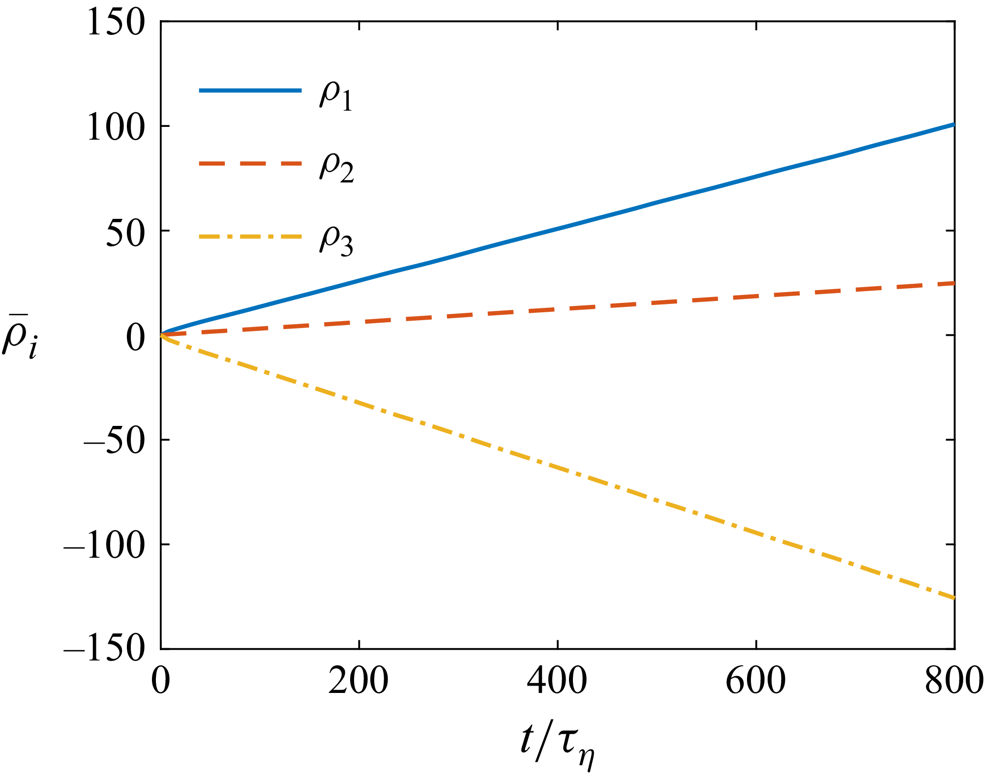
The spatial-averaged increasing/decreasing rates of the eigenvalues of
 $\unicode{x1D63E}$
with
 $\varLambda =1$
in
 $Re_\lambda \approx 90$
forced HIT flow.

According to (2.6)–(2.11), the orientation of the spheroid is closely related to the Cauchy–Green tensor
 $\unicode{x1D63E}$
. When spheroid orientations are fully developed in turbulent flow, i.e. when particle orientations become statistically stationary with respect to the fluid vorticity and the principal axes of the strain-rate tensor, the spatial-averaged rates of change in the eigenvalues of
 $\unicode{x1D63E}$
are nearly constant, as shown in figure 3. These constant rates of change are referred to as the Lyapunov exponents. Therefore, the spatially averaged Lyapunov exponents
 $\bar \sigma _i$
of spheroid orientations are given by
 \begin{align} \bar \sigma _i=\frac {\bar \rho _i(t_1)-\bar \rho _i(t_0)}{t_1-t_0}, \quad \text{where } i=1,2,3. \end{align}
Here, the bar represents a spatial average. The ensemble-averaged Lyapunov exponents
 $\langle \sigma _i \rangle$
of spheroid orientation can thus be expressed as
 \begin{align} \langle \sigma _i\rangle =\varLambda \langle \tilde {S}_{\textit{ii}}\rangle , \quad \text{where } i=1,2,3. \end{align}
Here, no summation is implied over the repeated index,
 $\tilde {{\unicode{x1D64E}}}$
is the fluid strain-rate tensor transformed by
 $\kern2pt \tilde {{\kern-2pt \unicode{x1D64E}}}={\unicode{x1D64D}}^{\rm T}\boldsymbol{\cdot }{\unicode{x1D64E}} \boldsymbol{\cdot }{\unicode{x1D64D}}$
, and
 $\langle {\cdot }\rangle$
represents both spatial and temporal ensemble averaging. Furthermore, the alignment factor
 $\bar \phi _p$
is approximately given by
 \begin{align} \bar {\phi }_p\sim \frac {{\rm e}^{2\langle \sigma _1\rangle t}}{{\rm e}^{2\langle \sigma _1\rangle t}+{\rm e}^{2\langle \sigma _2\rangle t}+{\rm e}^{2\langle \sigma _3\rangle t}}. \end{align}
For a given critical alignment factor
 $\phi _{pc}$
, the following relation holds:
 \begin{align} {\phi }_{pc}^{-1}-1={\rm e}^{2(\langle \sigma _2\rangle -\langle \sigma _1\rangle )t_\sigma } \big(1+{\rm e}^{2(\langle \sigma _3\rangle -\langle \sigma _2\rangle )t_\sigma } \big), \end{align}
where
 $t_\sigma$
is the time when
 $\bar \phi _p$
approaches the critical factor
 $\phi _{pc}$
. Note that subscript
 $\sigma$
indicates that the time is defined by Lyapunov exponents. Let
 $\varGamma _a=\langle \sigma _1\rangle -\langle \sigma _2\rangle$
,
 $\varGamma _b=\langle \sigma _2\rangle -\langle \sigma _3\rangle$
and
 $\vartheta _c=-\ln (\phi _{pc}^{-1}-1)$
. Equation (2.15) can thus be written as
 \begin{align} \vartheta _c=2\varGamma _a t_\sigma -\ln \big(1+{\rm e}^{-2\varGamma _b t_\sigma } \big). \end{align}
Here,
 $\varGamma _a\gt 0$
,
 $\varGamma _b\gt 0$
and
 $\vartheta _c\gt 0$
. Hence
 $\ln (1+{\rm e}^{-2\varGamma _b t_\sigma })\sim {\rm e}^{-2 \varGamma _b t_\sigma }\ll 1$
. When
 $\phi _{pc}\rightarrow 1$
, (2.16) simplifies to
 \begin{align} \vartheta _c\approx 2\varGamma _a t_\sigma . \end{align}
Therefore, the corresponding alignment time
 $t_\sigma$
may be approximated as
 \begin{align} t_\sigma \approx \frac {\vartheta _c}{2\varGamma _a}. \end{align}
Note that
 $\vartheta _c$
is a constant determined by the critical alignment factor
 $\phi _{pc}$
, thus
 $t_\sigma \sim 1/\varGamma _a$
. Here,
 $1/\varGamma _a$
can be viewed as a time scale, denoted as
 $\tau _\sigma$
, and
 $\tau _a$
is the statistical alignment response time obtained by averaging alignment time over individual trajectories, whereas
 $\tau _\sigma$
is estimated from the Lyapunov-based description. Consequently, the statistical alignment response time
 $\tau _a$
is not identical to
 $\tau _\sigma$
, but is of the same order of magnitude, i.e.
 \begin{align} \tau _a\sim \tau _\sigma =\frac {1}{\varGamma _a}. \end{align}
Here, the time scale
 $\tau _\sigma$
is independent of the critical alignment factor
 $\phi _{pc}$
. Nevertheless,
 $\tau _a$
and
 $\tau _\sigma$
are obtained from two fundamentally different approaches. The former is defined from the DNS alignment dynamics, whereas the latter is derived from the Lyapunov-exponent analysis. Therefore, their relationship requires further examination, which is presented in § 3.
3. Results and discussion
3.1. Alignment response time
 $\tau _a$

Response time versus shape parameter for (a) prolate and (b) oblate spheroids. The dashed lines correspond to the power-law slopes
 $-\xi _a=-1.760$
and
 $-\xi _a=-2.072$
, respectively. The corresponding power-law functions
 $\xi _a$
versus Taylor Reynolds number
 $Re_\lambda$
for prolate and oblate spheroids are shown in (c) and (d), respectively. Note that JHU represents the results computed via Johns Hopkins Turbulence Databases.

Figure 4 shows a clear power-law relationship between the alignment response time
 $\tau _a$
and the shape parameter
 $\varLambda$
for a critical alignment factor
 $\phi _{pc}=0.99$
, namely
 $\tau _a\sim |\varLambda |^{-\xi _a}$
. These power-law exponents of prolate and oblate spheroids at
 $Re_\lambda =90$
are
 $\xi _a=1.760$
and
 $\xi _a=2.072$
, respectively. As shown in figures 4(c) and 4(d), the exponents
 $\xi _a$
for prolate spheroids exhibit a noticeable dependence on
 $Re_\lambda$
, whereas the exponent for oblate spheroids remains nearly unchanged. With increasing
 $Re_\lambda$
,
 $\xi _a$
for prolate spheroids decreases to approximately 1.5, while the exponent for oblate spheroids remains close to 2. Zhao et al. (Reference Zhao, Gustavsson, Ni, Kramel, Voth, Andersson and Mehlig2019) found that the spheroid alignment is mainly driven by the stretching effect of the fluid strain rate that the particle experiences, and the shape parameter
 $\varLambda$
modifies the dominance of fluid strain rate on spheroid alignment relative to the rotation of fluid. In the present study, the relative importance of vorticity and the strain-rate eigenvectors is determined by the turbulent flow and is therefore independent of particle shape due to the one-way coupling assumption. The shape parameter instead modifies the strength of the strain-induced alignment. As
 $|\varLambda |$
decreases, the fluid strain-rate contribution is weakened relative to rotation, which effectively increases the delay in alignment with the strain-rate directions. By contrast, as
 $|\varLambda |$
increases, the strain contribution is enhanced, reducing the delay time, and leading to rapid alignment with the strain-rate eigenvectors. Moreover, as
 $|\varLambda |$
approaches zero (sphere), the stretching effect of the fluid strain rate vanishes, leading to an infinitely long response time for spheres. In the physical regime
 $|\varLambda |\lt 1$
, and even in the limiting case
 $|\varLambda |=1$
, the alignment with the strain-rate eigenvectors remains delayed relative to that of vorticity or material lines and surfaces. In addition, it is notable that the response time for prolate spheroids is slightly longer than that for oblate ones, suggesting that the sign of
 $\varLambda$
also affects spheroids alignments. For prolate spheroids (
 $\varLambda \gt 0$
), the symmetry axis preferentially aligns with the intermediate principal direction of the strain-rate tensor, similarly to vorticity and material lines. By contrast, the symmetry axis of oblate spheroids preferentially aligns with the most compressive principal direction of the strain-rate tensor, similar to the material surface. Since the magnitude of the compressive direction of the strain-rate tensor is statistically stronger than that associated with the intermediate principal direction, the alignment dynamics of oblate spheroids may differ from that of prolate spheroids. This difference provides a possible explanation for the different response times observed for prolate and oblate spheroids with the same value of
 $|\varLambda |$
.
As shown in figure 4, the alignment response time
 $\tau _a$
is derived for a single critical value
 $\phi _{pc}=0.99$
. To further explore the influence of
 $\phi _{pc}$
, we vary it over the range from 0.6 to 0.99, as depicted in figure 5. The results indicate that the power-law exponent
 $\xi _a$
is almost independent of
 $\phi _{pc}$
. From figure 5, it is clear that a reliable and
 $\phi _{pc}$
-independent power-law relationship can be obtained within the physical regime
 $|\varLambda | \lt 1$
, indicating a physical intrinsic relationship. As shown in figures 4 and 5, the anisotropic shape of spheroids inherently affects the alignment rate in turbulence as
 $|\varLambda |$
increases. Notably, even as the shape approaches a physical limit, i.e.
 $|\varLambda |=1$
, spheroids within a tiny fluid parcel still require a longer alignment time
 $\tau _a$
compared to the residence time scale
 $\tau _{\kern-1pt f}$
of the fluid particles staying within a small scale. Here,
 $\tau _{\kern-1pt f}$
is a statistical time by averaging the times that particle pairs remain in close proximity, i.e.
 $\tau _{\kern-1pt f} =\langle T_{\kern-1pt f}\rangle$
. According to Salazar & Collins (Reference Salazar and Collins2009),
 $\tau _{\kern-1pt f}\propto \tau _\eta$
within the dissipation subrange. This implies
 $\tau _a \gt \tau _{\kern-1pt f}$
for inertialess spheroids of any shape in turbulence, indicating that the flow varies on a time scale shorter than that required for alignment. Consequently, if the separation of two nearby spheroids is taken into account, then they are unlikely to align in the same direction.
Besides, according to figure 4, for the limiting case
 $\varLambda =1$
, the alignment response time is approximately
 $40\tau _\eta$
. The corresponding large-eddy turnover times for
 $Re_\lambda =30$
, 90, 170 and 418 are
 $6.75\tau _\eta$
,
 $12.55\tau _\eta$
,
 $22.31\tau _\eta$
and
 $46.93\tau _\eta$
, respectively. Therefore, the alignment response time of the limiting case
 $\varLambda =1$
exceeds the large-eddy turnover time for
 $Re_\lambda =30{-}170$
, while it becomes slightly smaller than the large-eddy turnover time at
 $Re_\lambda =418$
. For the case
 $\varLambda =-1$
, its alignment response time is approximately
 $20\tau _\eta$
, which is larger than the large-eddy turnover time for
 $Re_\lambda =30$
and
 $90$
, but smaller than that for
 $Re_\lambda =170$
and
 $418$
. These results indicate that during the alignment process, finite-aspect-ratio spheroids experience many different fluid structures in turbulence rather than remaining within a single coherent vortical structure. Consequently, the alignment process cannot be interpreted as the response of spheroids to an individual fluid structure. Instead, it reflects the cumulative effect of the evolving velocity-gradient field along a Lagrangian trajectory. The fact that the alignment response time is comparable to or even exceeds the large-eddy turnover time suggests that spheroid orientations retain memory of their initial conditions over long periods, highlighting the strong Lagrangian history effect of the alignment dynamics.
Response time
 $\tau _a/\tau _\eta$
and shape parameter
 $\varLambda$
plotted against different critical alignment factors
 $\phi _{pc}$
for (a) prolate and (b) oblate spheroids. The corresponding power-law functions
 $\xi _a$
versus alignment factors
 $\phi _{pc}$
are also shown in (c) and (d), respectively. The dashed lines in (a) and (b) indicate the power-law fits with slopes
 $-\xi _a=-1.760$
and
 $-\xi _a=-2.072$
, respectively.

3.2. Explanation from the Lyapunov exponents of spheroid orientation
According to the results shown in figures 4 and 5, two intriguing questions are what is the origin of the observed power-law relationship, and why are power laws of prolate and oblate spheroids different? In this subsection, we attempt to provide theoretical explanations.
Schematic of the spheroid Cauchy–Green tensor
 $\unicode{x1D63E}$
. (a,b) The physical shapes of prolate and oblate spheroids, respectively. (c,d) The geometries of the orientational Cauchy–Green tensors for prolate and oblate spheroids, respectively. (e,f) The corresponding Cauchy–Green tensors from different viewing perspectives.

First, the alignments of spheroids, described by the second-moment tensor
 $\unicode{x1D64B}$
of spheroids, are associated with the left Cauchy–Green tensor of spheroids; see (2.5) (Montgomery-Smith et al. Reference Montgomery-Smith, He, Jack and Smith2011; Cui & Zhao Reference Cui and Zhao2021). The closure between
 $\unicode{x1D64B}$
and
 $\unicode{x1D63E}$
, as well as the specific steps for calculating
 $\unicode{x1D64B}$
, are detailed in § 2.2. Second, we find that the eigenvalues of
 $\unicode{x1D63E}$
evolve exponentially with nearly stationary rates (see figure 3). This is attributed to the stationary correlation between the eigenvectors
 $\boldsymbol{e}_i\ (i=1,2,3)$
of
 $\unicode{x1D63E}$
and the principal axes of the fluid strain rate in turbulence. These stationary rates of increasing or decreasing of the eigenvalues of
 $\unicode{x1D63E}$
are inherently associated with the Lyapunov exponents. Specifically, the Lyapunov exponents of spheroid orientations over a time interval
 $[t_0, t_1]$
are defined as
 $\sigma _i=[\rho _i(t_1)-\rho _i(t_0)]/(t_1-t_0)$
, where
 $i=1,2,3$
,
 $2\rho _i(t)=\ln c_i$
, and
 $c_i$
represents the
 $i$
th eigenvalue of
 $\unicode{x1D63E}$
. In this study, the ensemble-averaged Lyapunov exponents for spheroids are given by
 \begin{align} \langle \sigma _i\rangle =\varLambda \langle \boldsymbol{e}_{i}^{\rm T} \boldsymbol{\cdot }{\unicode{x1D64E}}\boldsymbol{\cdot }\boldsymbol{e}_{i}\rangle ,\quad i=1,2,3, \end{align}
where
 $\langle \sigma _1\rangle \gt \langle \sigma _2\rangle \gt \langle \sigma _3\rangle$
and
 $\langle \sigma _1\rangle +\langle \sigma _2\rangle +\langle \sigma _3\rangle =0$
due to the fluid incompressibility. In general, prolate spheroids exhibit
 $\langle \sigma _2\rangle \gt 0$
, while oblate spheroids have
 $\langle \sigma _2\rangle \lt 0$
, owing to the statistically positive middle eigenvalue of fluid strain rate in turbulence, which tends to deform fluid material elements into a pancake. Note that due to the sign of
 $\varLambda$
,
 $\langle \sigma _1\rangle _{\varLambda =1}=-\langle \sigma _3\rangle _{\varLambda =-1}$
,
 $\langle \sigma _2\rangle _{\varLambda =1}=-\langle \sigma _2\rangle _{\varLambda =-1}$
and
 $\langle \sigma _3\rangle _{\varLambda =1}=-\langle \sigma _1\rangle _{\varLambda =-1}$
. According to (2.19), the alignment response time based on Lyapunov exponents is defined as
 $\tau _\sigma =1/\varGamma _a$
, where
 $\varGamma _a=\langle \sigma _1\rangle -\langle \sigma _2\rangle$
. Nonetheless,
 $\varGamma _a$
represents the difference between the largest and middle Lyapunov exponents of spheroids. This difference quantifies the stretching rate between the fastest and second-fastest deformation directions of
 $\unicode{x1D63E}$
. Figure 6 shows the geometric characteristics of the orientation Cauchy–Green tensor of spheroids. For prolate spheroids, the orientation Cauchy–Green tensor possesses two stretching directions and one contracting direction, resulting in a disk-like geometric representation, as shown in figure 6(c). By contrast, for oblate spheroids, the orientation Cauchy–Green tensor possesses one stretching direction and two contracting directions, giving rise to a rod-like geometric representation, as shown in figure 6(d). Figures 6(e) and 6(f) present different perspectives of the corresponding Cauchy–Green tensors, where the dashed lines denote the initial spherical configuration. These perspectives illustrate the deformation of the orientation Cauchy–Green tensor over time, and highlight the distinct stretching and contraction characteristics associated with prolate and oblate spheroids.
(a) Relationship between the Lyapunov-description alignment response time
 $\tau _\sigma$
and the shape parameter
 $|\varLambda |$
of spheroids. The dashed lines represent the corresponding fitted curves, while the dash-dotted line refers to (3.2) with
 ${Ku}=0.2$
.(b) The corresponding power-law functions
 $\zeta _\sigma$
versus Taylor Reynolds number
 $Re_\lambda$
for prolate and oblate spheroids.

In this subsection, we examine the relationship given by (2.19), namely
 $\tau _a\sim \tau _\sigma$
. Figure 7(a) shows that
 $\tau _\sigma$
also exhibits a power-law dependence on the shape parameter, i.e.
 $\tau _\sigma \sim |\varLambda |^{-\zeta _\sigma }$
. The exponent
 $\zeta _\sigma$
is found to be close to the exponent
 $\xi _a$
obtained from the scaling of the alignment response time
 $\tau _a$
. Additionally, the difference between prolate and oblate spheroids observed in
 $\zeta _\sigma$
is consistent with that found for
 $\xi _a$
. The agreement between these two power-law exponents is particularly noteworthy because they are obtained from two independent approaches. The exponent
 $\xi _a$
is determined directly from DNS by fitting the dependence of the ensemble-averaged response time on the shape parameter, whereas
 $\zeta _\sigma$
is derived from the Lyapunov-exponent analysis of spheroid orientation dynamics. The close agreement demonstrates that the scaling behaviour of the alignment response time can be explained by the dependence of the Lyapunov-exponent difference
 $\varGamma _a$
on the shape parameter. It also suggests that
 $\tau _\sigma$
provides a physically meaningful alignment time scale that is independent of the critical threshold. Therefore, the power law between
 $\tau _a$
and
 $|\varLambda |$
can be directly illustrated via the power law of
 $\tau _\sigma$
versus
 $|\varLambda |$
, as shown in figure 7(a). According to the definition (2.19), similar power laws between
 $\tau _\sigma$
and
 $|\varLambda |$
can be observed in random flows, specifically in isotropic, homogeneous Gaussian random velocity fields (Byron et al. Reference Byron, Einarsson, Gustavsson, Voth, Mehlig and Variano2015; Gustavsson & Mehlig Reference Gustavsson and Mehlig2016). The corresponding
 $\varGamma _a$
is expressed as
 \begin{align} \quad \varGamma _a \tau =\langle \sigma _1\rangle \tau \approx 2\,\textit{Ku}^2\varLambda ^2-\textit{Ku}^4\varLambda ^2 \big(9\varLambda ^2+16 \big)/3, \end{align}
where
 $\textit{Ku}=u_0\tau /\eta$
, with
 $u_0$
representing the intensity of velocity fluctuations in random flows, and
 $\eta$
and
 $\tau$
being the correlation length and time scales of random flows, respectively. The Kubo number
 $\textit{Ku}$
is a dimensionless measure of how rapidly the fluid velocity fluctuates (Gustavsson & Mehlig Reference Gustavsson and Mehlig2016);
 $\textit{Ku}\rightarrow 0$
represents a white-noise limit. According to (3.2),
 $\varGamma _a\sim \varLambda ^2$
when
 $\textit{Ku}\ll 1$
. Nonetheless, the relationships between
 $\varGamma _a$
and
 $|\varLambda |$
of prolate and oblate spheroids are the same, because the middle Lyapunov exponent
 $\langle \sigma _2\rangle$
is always zero in the random flow employed by Byron et al. (Reference Byron, Einarsson, Gustavsson, Voth, Mehlig and Variano2015) and Gustavsson & Mehlig (Reference Gustavsson and Mehlig2016). Note that in Gaussian random flows, the velocity-gradient fields do not exhibit preferential strain structures, and the correlation between vorticity and strain rate is absent.
Although HIT differs from random flows, the
 $-2$
power-law relationship between the response time
 $\tau _\sigma$
and shape parameter
 $|\varLambda |$
of spheroids in the random flow can help us to understand the power-law relationship in HIT. In HIT, the middle eigenvalue of the fluid strain rate is statistically positive, which indicates that the strain structure tends to be axisymmetric, with extension in two directions, and compression in the third (Ashurst et al. Reference Ashurst, Kerstein, Kerr and Gibson1987; Meneveau Reference Meneveau2011). This is in contrast to the random flow where the middle eigenvalue of the strain rate is zero, corresponding to non-preferred strain structures. Despite spheroids having preferential alignments in the eigenframe of the strain-rate tensor, these alignments are not perfect in HIT, leading to a non-zero middle Lyapunov exponent (Guala et al. Reference Guala, Liberzon, Lüthi, Kinzelbach and Tsinober2006). This causes
 $\varGamma _a$
of prolate spheroids to be slightly smaller than that of oblate ones, because of the statistically positive (negative) middle Lyapunove exponent of prolate (oblate) spheroids, as illustrated in figure 6.
Additionally, the non-zero middle Lyapunov exponent of spheroids is also related to the shape parameter, which finally affects the power laws
 $\zeta _\sigma$
for the alignment response time. An interesting observation in the present results is that the theoretical model predicts the power-law behaviour of oblate spheroids reasonably well, whereas deviations are observed for prolate spheroids. To illustrate this phenomenon, we further examined this from the viewpoint of the Cauchy–Green tensor associated with the orientation dynamics, as shown in figure 6, because the Cauchy–Green tensor directly reflects the orientation of the symmetry axes of spheroids. For prolate spheroids
 $(\varLambda \gt 0)$
, the corresponding orientation Cauchy–Green tensor possesses two stretching directions and one contracting direction. This structure resembles the deformation of fluid elements in turbulence, and is closely related to the statistically positive value of the intermediate principal strain-rate eigenvalue. In contrast, for oblate spheroids
 $(\varLambda \lt 0)$
, the sign of
 $\varLambda$
leads to an opposite structure of the orientation Cauchy–Green tensor compared with that of prolate spheroids having the same
 $|\varLambda |$
, namely one stretching direction and two contracting directions. Since the alignment dynamics is primarily governed by stretching directions, the number of stretching directions plays a key role in determining the alignment response. In an ideal random flow, the intermediate strain-rate eigenvalue is statistically zero, implying that fluid elements evolve effectively with one stretching direction, one neutral direction and one contracting direction. Under such conditions, the orientation Cauchy–Green tensors of both prolate and oblate spheroids effectively possess only one stretching direction, resulting in a symmetric alignment behaviour and identical scaling exponents. However, the situation is different in turbulence. Owing to the statistically positive intermediate strain-rate eigenvalue, the second stretching direction of the prolate orientation Cauchy–Green tensor becomes active, whereas the orientation Cauchy–Green tensor of oblate spheroids still retains only one stretching direction. Consequently, the orientation dynamics of oblate spheroids remains closer to that predicted in random flows, while that of prolate spheroids deviates from the results in random flows. We therefore believe that this asymmetry in the stretching structure of the orientation Cauchy–Green tensor provides a plausible explanation for why the scaling exponent
 $\zeta _\sigma$
of prolate spheroids differs from the random-flow prediction, whereas that of oblate spheroids remains much closer to it.
To support this explanation, we show the time evolution of the ensemble-averaged eigenvalues of
 $\unicode{x1D64B}$
using the Lyapunov exponents
 $\langle \sigma _i\rangle\ (i=1,2,3)$
related to the orientation Cauchy–Green tensors, i.e.
 \begin{align} \begin{split} \langle \tilde {P}_{11}\rangle &=\frac {1}{2}\int _{0}^{\infty }\frac {\mathrm{d}s}{(\textrm{e}^{-2\langle \sigma _1\rangle t}+s)^{3/2}\sqrt {\textrm{e}^{-2\langle \sigma _2\rangle t}+s}\sqrt {\textrm{e}^{-2\langle \sigma _3\rangle t}+s}},\\[5pt]\langle \tilde {P}_{22}\rangle &=\frac {1}{2}\int _{0}^{\infty }\frac {\mathrm{d}s}{(\textrm{e}^{-2\langle \sigma _2\rangle t}+s)^{3/2}\sqrt {\textrm{e}^{-2\langle \sigma _3\rangle t}+s}\sqrt {\textrm{e}^{-2\langle \sigma _1\rangle t}+s}},\\[5pt]\langle \tilde {P}_{33}\rangle &=\frac {1}{2}\int _{0}^{\infty }\frac {\mathrm{d}s}{(\textrm{e}^{-2\langle \sigma _3\rangle t}+s)^{3/2}\sqrt {\textrm{e}^{-2\langle \sigma _1\rangle t}+s}\sqrt {\textrm{e}^{-2\langle \sigma _2\rangle t}+s}}.\\ \end{split} \end{align}
Time evolution of the eigenvalues of the orientational second-moment tensors
 $\unicode{x1D64B}$
of (a–c) prolate and (d–f) oblate spheroids. The three ensemble-averaged eigenvalues of
 $\unicode{x1D64B}$
correspond to (a,d)
 $\langle \tilde {P}_{11}\rangle$
, (b,e)
 $\langle \tilde {P}_{22}\rangle$
and (c,f)
 $\langle \tilde {P}_{33}\rangle$
. Solid lines are computed using the statistic Lyapunov exponents measured in DNS, while dashed lines are obtained using Lyapunov exponents predicted for Gaussian random flow. The horizontal black dotted lines mark the isotropic value
 $1/3$
.

Reynolds number effect of the evolution of the second eigenvalues of the orientational second-moment tensors
 $\langle \tilde {P}_{22}\rangle$
for (a) prolate and (b) oblate spheroids. Solid, dashed, dash-dotted and symbol-connected lines denote
 $Re_\lambda =418$
,
 $170$
, 90 and 30, respectively. The horizontal black dotted lines mark the isotropic value
 $1/3$
.

For the DNS results, the Lyapunov exponents of prolate spheroids satisfy
 $\langle \sigma _1\rangle \gt \langle \sigma _2\rangle \gt 0\gt \langle \sigma _3\rangle$
, whereas those of oblate spheroids satisfy
 $\langle \sigma _1\rangle \gt 0\gt \langle \sigma _2\rangle \gt \langle \sigma _3\rangle$
. However, for Gaussian random flows, the Lyapunov exponents satisfy
 $\langle \sigma _1\rangle \gt \langle \sigma _2\rangle =0\gt \langle \sigma _3\rangle$
and
 $\langle \sigma _1\rangle =-\langle \sigma _3\rangle$
for both prolate and oblate spheroids. This fundamental difference reflects the distinct stretching properties of real turbulence and Gaussian random flows. To facilitate a meaningful comparison with turbulence, the Lyapunov exponents of the Gaussian random flow are chosen such that their overall magnitude matches that of the DNS results. Specifically, the Lyapunov exponents of the random flow satisfy
 $\langle \sigma _1\rangle _{\textit{random}}=\sqrt {(\langle \sigma _1\rangle _{\textit{turb}}^2+\langle \sigma _2\rangle _{\textit{turb}}^2+\langle \sigma _3\rangle _{\textit{turb}}^2)/2}$
, where subscript
 $\textit{turb}$
denotes the corresponding values obtained from turbulence. Consequently, figure 8 shows that
 $\langle \tilde {P}_{22}\rangle \gt 1/3$
during the early stage of the alignment process for prolate spheroids with large aspect ratios. This indicates that the intermediate stretching direction of the Cauchy–Green tensor contributes to the alignment process, giving rise to two preferential alignment directions during the initial stage. As the alignment process proceeds, the influence of the intermediate stretching direction gradually diminishes, and the corresponding eigenvalue eventually falls below the isotropic value
 $1/3$
. Moreover, this effect becomes progressively weaker as
 $\varLambda$
approaches zero and vanishes in the spherical limit. In contrast, oblate spheroids exhibit only a single preferential alignment direction throughout the whole evolution. This behaviour is consistent with that predicted for random flows, where the intermediate Lyapunov exponent is identically zero, and only one dominant stretching direction governs the alignment process. As a result, the evolution of the ensemble-averaged eigenvalues of
 $\unicode{x1D64B}$
for oblate spheroids in Gaussian random flows closely resembles that observed in turbulence, as shown in figures 8(d–f). This suggests that oblate spheroids are less sensitive to the intermediate Lyapunov exponent present in turbulence, whereas the alignment dynamics of prolate spheroids is more strongly affected by this additional stretching direction.
Besides, the Reynolds number dependence of the power-law exponent
 $\zeta _\sigma$
governing the scaling between
 $\tau _\sigma$
and
 $\varLambda$
is shown in figure 7(b). The behaviour is consistent with that observed for
 $\xi _a$
: as
 $Re_\lambda$
increases, the exponent
 $\zeta _\sigma$
for prolate spheroids decreases, whereas the exponent
 $\zeta _\sigma$
for oblate spheroids remains close to 2. The discrepancy becomes more pronounced with increasing Reynolds number, reflecting the growing influence of the non-Gaussian characteristics of turbulence. As the Reynolds number increases, intermittency becomes stronger, and the statistics of the velocity-gradient tensor depart further from those of an ideal Gaussian random flow, leading to more pronounced preferential strain-rate structures. Consequently, the influence of the intermediate stretching direction on the orientation dynamics of prolate spheroids is enhanced. As shown in figure 9(a), this effect causes
 $\langle \tilde {P}_{22}\rangle$
to remain above the isotropic value
 $1/3$
for a longer period as Reynolds number increases, leading to an increasing deviation from the random-flow prediction. In contrast, the evolution of
 $\langle \tilde {P}_{22}\rangle$
for oblate spheroids in figure 9(b) exhibits only a weak dependence on Reynolds number.
4. Conclusion
In this study, we introduce the concept of the alignment response time, which quantifies the time it takes for spheroids with random initial orientations to align in a certain direction along their particle trajectories. Our findings reveal that the response time exhibits a power-law relationship with the shape parameter of spheroids. In particular, the exponent for oblate spheroids is approximately
 $-2$
, whereas the exponent for prolate spheroids deviates slightly and exhibits a dependence on the Reynolds number
 $Re_\lambda$
.
We propose that this power law arises from the relationship between the difference in the maximum and middle Lyapunov exponents of spheroids and their shape parameter. This reflects the disparity in stretching rates between the fastest and second-fastest directions of the deformation rate tensor of spheroid orientation. The difference in power-law exponents between prolate and oblate spheroids can be attributed to the statistical properties of the fluid strain rate in turbulence, particularly the positive middle eigenvalue of the fluid strain-rate tensor, which is associated with the non-Gaussian characteristics of turbulence.
Moreover, the inverse relationship between the response time and
 $\varGamma _a$
, i.e. the difference of the maximum Lyapunov exponent to the middle Lyapunov exponent of spheroids, furnishes a novel and efficient way to estimate the aligning processes of spheroids in turbulence. If this relationship is also confirmed in inhomogeneous turbulent flows, such as jet and wall-bounded flows, then we believe that
 $\tau _\sigma =1/\varGamma _a$
should be a powerful tool to estimate the characteristic time of the spheroid alignment in turbulence. This method is also a benefit in estimating how long the spheroid orientations are fully developed and independent of initial distribution of orientations.
In addition, the present study is restricted to a dilute particle phase, and interactions among the particles are neglected. In future work, particle separation dynamics and particle–particle collisions will be considered. Furthermore, theoretical models accounting for the influence of turbulent intermittency and the non-Gaussian velocity-gradient statistics on spheroid alignment warrant further investigation.
Funding
This work was supported by the Natural Science Foundation of China (grant nos 12302285, 12532011 and 12388101), the Hunan Provincial Natural Science Foundation of China (grant no. 2026JJ40004), and the Fundamental Research Funds for the Central Universities. This work is also funded by State Key Laboratory of Advanced Space Propulsion (No. 2025ASP0101).
Declaration of interests
The authors report no conflict of interest.
AI transparency statement
ChatGPT was used to improve the English language of the manuscript, including grammar correction, word choice and sentence structure. All scientific content, code, analyses and conclusions were conducted by the authors.
Appendix A. Validity of the computation method for the orientational moment tensor
To assess the validity and efficiency of the present method (see § 2.2), we compare its predictions with those obtained by an analytical solution (Okagawa et al. Reference Okagawa, Cox and Mason1973) and the results from explicit ensemble averaging in a simple shear flow,
 $\boldsymbol{u} =[\kappa y,0,0]^{\rm T}$
, where
 $\kappa$
denotes the shear rate. In the analytical approach, the orientation moment tensor is evaluated as
 \begin{align} {\unicode{x1D64B}}(t)=\langle \boldsymbol{n} \boldsymbol{n} \rangle _{\psi }(t) =\iint _S \boldsymbol{n} \boldsymbol{n} \psi\, \mathrm{d} S(\boldsymbol{n}), \end{align}
where
 $\psi$
is the probability density function of particle orientation, initially uniform, given by
 \begin{align} \psi =\frac {1}{4\pi \big[\cos ^2\theta +\beta ^2 \sin ^2\theta \big]^{3/2}}. \end{align}
Here,
 \begin{align} \begin{split} \beta ^2&=\beta _1\sin ^2\varphi +\dfrac {1}{2}\beta _2 \sin 2\varphi +\beta _3 \cos ^2\varphi , \\[3pt]\beta _1&=\frac {1}{2}\left [1+\lambda ^{-2}+ \big(1-\lambda ^{-2} \big)\cos \frac {4\pi t}{T_J}\right ], \\[3pt]\beta _2&= \big(\lambda ^{-1}-\lambda \big)\sin \frac {4\pi t}{T_J},\\[3pt]\beta _3&=\frac {1}{2}\left [1+\lambda ^{2}+ \big(1-\lambda ^{2} \big)\cos \frac {4\pi t}{T_J}\right ], \end{split} \end{align}
where
 $\theta$
,
 $\varphi$
are the zenithal and azimuthal angles of spherical coordinates, respectively, and
 $T_J=2\pi (\lambda + \lambda ^{-1})/\kappa$
is the Jeffery period.
Time evolution of the second moment tensor
 $P_{\textit{ij}}=\langle n_i n_{\kern-1pt j}\rangle$
of spheroid orientation with
 $\lambda =5$
in a simple shear flow.

Figure 10. Long description
The image contains four line graphs labeled (a), (b), (c), and (d). Each graph plots the second moment tensor of spheroid orientation over time in a simple shear flow. The x-axis for all graphs is labeled with ‘κt’ and ranges from 0 to 30. Panel A: The y-axis is labeled with ‘<n1n1>’ and ranges from 0.3 to 0.9. The graph shows multiple lines representing different methods and particle counts, with data points marked by circles. The lines exhibit a periodic trend with peaks and troughs. Panel B: The y-axis is labeled with ‘<n2n2>’ and ranges from 0 to 0.35. Similar to Panel A, this graph also shows multiple lines with periodic trends. Panel C: The y-axis is labeled with ‘<n3n3>’ and ranges from 0.14 to 0.34. The graph displays periodic trends with peaks and troughs, represented by multiple lines. Panel D: The y-axis is labeled with ’<n1n2>’ and ranges from -0.20 to 0.20. This graph also shows periodic trends with multiple lines.
For comparison, the moment tensor obtained by explicit ensemble averaging along the same trajectory is computed as
 \begin{align} {\unicode{x1D64B}}(t)=\langle \boldsymbol{n} \boldsymbol{n} \rangle _{\psi }(t) =\frac {1}{N_p} \sum _{i=1}^{N_p}\boldsymbol{n}^{(i)} \boldsymbol{n}^{(i)} , \end{align}
where
 $N_p$
is the number of particles. Three ensemble sizes are considered,
 $N_p=100, 1000, 5000$
.
To ensure a consistent comparison, all methods employ the same time step
 $\Delta t=T_J/5000$
. At each time step, the moment tensor is evaluated using the respective approach. The temporal evolution of the components of
 $\unicode{x1D64B}$
is shown in figure 10. The results obtained using the present method are in an excellent agreement with the analytical solution, whereas the ensemble-averaging approach exhibits noticeable deviations that decrease with increasing
 $N_p$
.
We further compare the evolution of corresponding alignment factor
 $\phi _p$
in figure 11. The predictions of the present method collapse onto the analytical solution, while those obtained from explicitly ensemble-averaging show pronounced deviations. The mean absolute errors of alignment factor
 $\phi _p$
over one Jeffery period, relative to the analytical solution, are summarised in table 1, confirming that the present method achieves high accuracy. The computational costs of the different approaches are also listed in table 1. The present method is the most efficient, whereas the explicit ensemble-averaging method requires a large number of particles and incurs the highest computational cost.
Accuracy and efficiency of different methods for computing the second-moment tensor of spheroid orientation.

Table 1. Long description
A table comparing errors and time costs of different methods for computing the second-moment tensor of spheroid orientation. The table has 2 rows and 5 columns. The columns are labeled as Methods, Analytical, Present, 100 particles, 1000 particles, and 5000 particles. The rows are labeled as Errors and Time costs. Row 1: Methods, Analytical, Present, 100 particles, 1000 particles, 5000 particles. Row 2: Errors, --, 0.0038, 0.0112, 0.0067, 0.0046. Row 3: Time costs, 501.08 s, 0.65 s, 3.96 s, 41.15 s, 199.29 s.
Time evolution of the alignment factors
 $\phi _p$
in a simple shear flow.

In conclusion, the method for computing the moment tensor described in § 2.2 exhibits both high accuracy and computational efficiency. It is therefore well suited for the present study, which requires evaluating the orientation statistics along a large number of Lagrangian trajectories in turbulence.

 Λ=0.8
 Reλ≈90
 Np=50
 ϕp
 ϕp=0
 ϕp=1

 ϕp
 Reλ≈90
 𝘾
 Λ=1
 Reλ≈90

 −ξa=−1.760
 −ξa=−2.072
 ξa
 Reλ

 τa/τη
 Λ
 ϕpc
 ξa
 ϕpc
 −ξa=−1.760
 −ξa=−2.072

 𝘾

 τσ
 |Λ|
 Ku=0.2
 ζσ
 Reλ

 𝙋
 𝙋
 ⟨P~11⟩
 ⟨P~22⟩
 ⟨P~33⟩
 1/3

 ⟨P~22⟩
 Reλ=418
 170
 1/3

 Pij=⟨ninj⟩
 λ=5


 ϕp


