1 Introduction
The flow connecting a thin liquid film with a static meniscus first emerged in the context of dip coating: in the classic set-up investigated by Landau & Levich (Reference Landau and Levich1942), the film is deposited on a plate which is gradually withdrawn from a reservoir of liquid. This set-up received a lot of attention later on. In particular, Wilson (Reference Wilson1982) demonstrated that the problem considered by Landau and Levich boils down to the asymptotic matching of a thin liquid film with a static meniscus. Besides that, numerous extensions of the Landau and Levich analysis were developed. Dip coating was considered in the presence of soluble (Krechetnikov & Homsy Reference Krechetnikov and Homsy2006; Campana et al. Reference Campana, Ubal, Giavedoni and Saita2010) and insoluble surfactants (Park Reference Park1991); the case of significant interface elasticity was considered by Dixit & Homsy (Reference Dixit and Homsy2013), whereas the theory of dip coating for non-Newtonian liquids was developed by Spiers, Subbaraman & Wilkinson (Reference Spiers, Subbaraman and Wilkinson1975) and Afanasiev, Münch & Wagner (Reference Afanasiev, Münch and Wagner2007). For a general review of coating flows see the papers of Ruschak (Reference Ruschak1985) and Weinstein & Ruschak (Reference Weinstein and Ruschak2004) and for an extensive review on coating fibres see the work of Quéré (Reference Quéré1999).
The propagation of a long bubble through a capillary filled with liquid can be also considered as a coating process. In his classical analysis, Bretherton (Reference Bretherton1961) arrived to the Landau–Levich equation while investigating the flow connecting the tip of the bubble with the thin liquid film sandwiched between the bubble and the capillary wall. Bretherton’s analysis, corresponding to the limit of small capillary number, was extended by Park & Homsy (Reference Park and Homsy1984), who obtained a higher-order correction to the thickness of the deposited film. Another extension of Bretherton’s analysis, valid for moderate capillary numbers, was developed by Klaseboer, Gupta & Manica (Reference Klaseboer, Gupta and Manica2014). Bretherton’s results were extensively checked experimentally (Schwartz, Princen & Kiss Reference Schwartz, Princen and Kiss1986; Aussillous & Quéré Reference Aussillous and Quéré2000). On a different note, the propagation of long bubbles through capillaries of a polygonal cross-section was first considered by Wong, Radke and Morris who adopted the language of matched asymptotic expansions to describe the deposition and rearrangement of the thin liquid film on the channel walls (Wong, Radke & Morris Reference Wong, Radke and Morris1995a ,Reference Wong, Radke and Morris b ). A review of the mathematical models of confined bubbles can be found in the paper by Ajaev & Homsy (Reference Ajaev and Homsy2006), and a discussion on bubbles in the more general context of microfluidics can be found in the review by Huerre, Miralles & Joullien (Reference Huerre, Miralles and Joullien2014).
The aim of this paper is to adapt the ideas stemming from the work of Landau and Levich to the world of acustofluidics. Recent experimental observations and theoretical investigations revealed that the excitation of thin liquid films by MHz-frequency surface acoustic waves (SAW) results in complex fluid flows (Rezk et al. Reference Rezk, Manor, Friend and Yeo2012, Reference Rezk, Manor, Yeo and Friend2014; Altshuler & Manor Reference Altshuler and Manor2015, Reference Altshuler and Manor2016; Manor, Rezk, Friend & Yeo Reference Manor, Rezk, Friend and Yeo2015) exhibiting fingering instabilities (Rezk et al. Reference Rezk, Manor, Friend and Yeo2012), solitary-like waves (Rezk et al. Reference Rezk, Manor, Friend and Yeo2012) and flow reversal (Rezk et al. Reference Rezk, Manor, Yeo and Friend2014; Manor et al. Reference Manor, Rezk, Friend and Yeo2015). It was also shown that the lubrication approximation combined with the multiscale asymptotic expansion of the equations describing the fluid flow due to SAW results in a thin-film evolution equation governing the large-scale dynamics of the film (Altshuler & Manor Reference Altshuler and Manor2015, Reference Altshuler and Manor2016; Manor et al. Reference Manor, Rezk, Friend and Yeo2015). For a general review of microfluidic phenomena driven by surface acoustic waves see the work of Friend & Yeo (Reference Friend and Yeo2011).
None of the theoretical models of the coating flows cited above consider the flow driven by acoustofluidic forces. In this paper we demonstrate that a Rayleigh SAW propagating in the solid substrate may generate a coating flow in a thin liquid film lying atop the substrate. We adopt the approach developed by Altshuler & Manor (Reference Altshuler and Manor2015) and derive the thin-film evolution equation governing the dynamics of the liquid film under the action of the propagating SAW. We then show that in a steady state the evolution equation reduces to a generalized Landau–Levich equation with the dragging velocity depending on the film thickness. In order to investigate the system dynamics, we carry out numerical analysis of both steady states and time-dependent solutions of the thin-film evolution equation. We expect that the theoretical predictions obtained in the present paper will provide additional insight into the interaction of SAW with thin liquid films and guide corresponding experimental work in the field of SAW assisted coating flows.
This paper is organized as follows. In § 2, we present the problem statement, review the derivation of the thin-film evolution equation and obtain the generalized Landau–Levich equation, which we study in § 3. In § 4 we explore the numerical stability of the steady states and the time-dependent solutions of the evolution equation. We discuss our theoretical predictions in § 5.
2 Thin-film equation
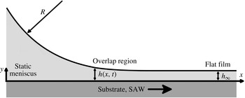
We investigate the interaction of a Rayleigh SAW with a thin liquid film lying atop a solid substrate, as shown in figure 1. Specifically, we demonstrate that a SAW propagating in the solid substrate may support a dip coating-like flow in the liquid film. In this section we discuss the problem statement and employ the lubrication approximation to obtain an extension of the Landau–Levich equation in the case of dragging a liquid film by a propagating Rayleigh SAW.
Sketch of the physical system under consideration: a flat liquid film of the constant thickness
 $h_{\infty }$
is dragged out of a static meniscus with curvature
 $R^{-1}$
. The aim of the present analysis is to describe the overlap region where the flow from the meniscus is matched with the flow in the flat film (Wilson Reference Wilson1982).

The flow geometry presented in figure 1 emerges in several different contexts. It is observed in coating processes, for instance, in blade coating where the typical set-up comprises a channel ending with a sharp corner (Ruschak Reference Ruschak1985; Weinstein & Ruschak Reference Weinstein and Ruschak2004). Further, the flow connecting a static meniscus with a thin liquid film develops naturally around a long bubble propagating through a capillary filled with liquid. In the case of a circular capillary, this type of flow appears near the tip of the bubble (Bretherton Reference Bretherton1961). In the case of a polygonal capillary, a similar flow corresponds to the rearrangement of liquid in the cross-sectional plane of the capillary (Wong et al.
Reference Wong, Radke and Morris1995a
). The flow geometry considered in this paper constitutes two separate mathematical problems: the outer problem, corresponding to the meniscus, and the inner problem, corresponding to the thin liquid film dragged out of the meniscus (Wilson Reference Wilson1982). For the sake of simplicity, we consider the inner problem, assuming that the solution of the outer problem yields a meniscus with a constant radius of curvature
 $R$
.
We further note that the assumption of a meniscus with a constant radius of curvature,
 $R$
, implies that the acoustic radiation pressure on the free surface of the liquid (Beyer Reference Beyer1974; Lee & Wang Reference Lee and Wang1993), exerted by sound waves leaking (diffracting) off the propagating SAW and impinging on the free surface of the liquid, is negligible compared to the Laplace pressure in the liquid due to the curvature of the meniscus. This assumption is satisfied by the requirement that
 $R\ll 2\unicode[STIX]{x1D6FE}(\unicode[STIX]{x1D70C}U^{2})^{-1}(1+B/2A)^{-1}$
, where
 $\unicode[STIX]{x1D70C}$
is the density of the liquid,
 $U$
is the displacement velocity of the substrate due to the SAW (characteristic values associated with SAW microfluidic platforms are between
 $1{-}1000~\text{mm}~\text{s}^{-1}$
) and
 $B/A$
is the nonlinearity parameter in the relation between pressure and density in liquid (characteristic values are between 1–10). For example, exciting water, satisfying
 $\unicode[STIX]{x1D70C}\approx 1000~\text{g}~\text{cm}^{-3}$
and
 $\unicode[STIX]{x1D6FE}\approx 70~\text{mN}~\text{m}^{-1}$
, by a SAW, supporting
 $U\approx 100~\text{mm}~\text{s}^{-1}$
, requires the radius of curvature of the meniscus to satisfy
 $R\ll 10~\text{mm}$
, such that the contributions from the acoustic radiation pressure are small. Further details are given in appendix A.
2.1 Problem statement
We consider a Rayleigh SAW, propagating along the
 $x$
-coordinate, in an isotropic solid substrate under a liquid film. At rest the solid is at
 $y\leqslant 0$
, as shown in figure 1. The SAW supports in-plane,
 $X(x,y,t)$
, and out-of-plane,
 $Y(x,y,t)$
, displacements of a similar magnitude along and transverse to the solid surface, respectively. We consider the limit of small displacements, where the ratio between the characteristic magnitude of the displacements,
 $U/\unicode[STIX]{x1D714}$
, and the length scale of the SAW in the solid,
 $k^{-1}$
, is small, such that
 $\unicode[STIX]{x1D701}\equiv (U/\unicode[STIX]{x1D714})/k^{-1}\ll 1$
; the quantities
 $U$
,
 $\unicode[STIX]{x1D714}$
and
 $k$
are the characteristic velocity of the displacements, the angular frequency and the wavenumber of the SAW, respectively. An asymptotic approximation of the velocity at the deforming solid surface may then be given in the form (Spencer Reference Spencer1970; Parker Reference Parker1988),
 $$\begin{eqnarray}\displaystyle (X_{t},Y_{t})|_{y=Y}=(X_{1,t},Y_{1,t})|_{y=0}+\unicode[STIX]{x1D701}(X_{2,t},Y_{2,t})|_{y=0}+\cdots \,, & & \displaystyle\end{eqnarray}$$
where
 $t$
is time,
 $Y$
is the out-of-plane displacement of the solid surface with respect to its position at rest,
 $X_{1}$
,
 $X_{2}$
,
 $Y_{1}$
, and
 $Y_{2}$
etc. are components of a similar magnitude in the asymptotic series that represent
 $X$
and
 $Y$
and additional subscripts denote corresponding partial derivatives; for example,
 $X_{1,t}\equiv \unicode[STIX]{x2202}X_{1}/\unicode[STIX]{x2202}t$
. The theory of linear elasticity gives the leading-order term in the expansion (2.1) (Wilmanski & Albers Reference Wilmanski and Albers2014),
 $$\begin{eqnarray}\displaystyle (X_{1,t},Y_{1,t})|_{y=0}=U[\cos (\unicode[STIX]{x1D714}t-kx),\unicode[STIX]{x1D712}\sin (\unicode[STIX]{x1D714}t-kx)], & & \displaystyle\end{eqnarray}$$
where
 $\unicode[STIX]{x1D712}\approx 1.3$
is the magnitude ratio between the in-plane and the out-of-plane displacements of the solid surface. Further details are given in appendix B.
The corresponding dimensional boundary condition for the flow above the solid surface reads then,
 $$\begin{eqnarray}\displaystyle (u,v)|_{y=0}=U[\cos (\unicode[STIX]{x1D714}t-kx),\unicode[STIX]{x1D712}\sin (\unicode[STIX]{x1D714}t-kx)]+O(U\unicode[STIX]{x1D701}), & & \displaystyle\end{eqnarray}$$
where
 $u$
and
 $v$
are the velocities of the fluid along the
 $x$
and
 $y$
coordinates, respectively.
We further impose the kinematic boundary condition and the balance of stresses at the free surface of the liquid film, namely,
 $$\begin{eqnarray}\displaystyle & \displaystyle h_{t}+uh_{x}=v\quad \text{at }y=h(x,t), & \displaystyle\end{eqnarray}$$
 $$\begin{eqnarray}\displaystyle & \displaystyle \unicode[STIX]{x1D64F}\boldsymbol{\cdot }\boldsymbol{n}+\unicode[STIX]{x1D6FE}\unicode[STIX]{x1D705}\boldsymbol{n}=0\quad \text{at }y=h(x,t), & \displaystyle\end{eqnarray}$$
 $h(x,t)$
is the thickness of the film,
 $\unicode[STIX]{x1D64F}$
is the stress tensor in the liquid,
 $\boldsymbol{n}$
is the outward unit normal vector to the free surface and
 $\unicode[STIX]{x1D6FE}$
and
 $\unicode[STIX]{x1D705}$
are the surface tension and mean curvature of the free surface.
Finally, we note that the typical thickness of the liquid film under consideration is assumed small compared to the wavelength of the applied SAW,
 $h\ll k^{-1}$
, such that compressional effects in the liquid may be ignored (Rezk et al.
Reference Rezk, Manor, Friend and Yeo2012, Reference Rezk, Manor, Yeo and Friend2014). In the absence of compressibility effects the continuity and the Navier–Stokes equations can be rewritten in terms of a streamfunction as follows,
 $$\begin{eqnarray}\displaystyle \unicode[STIX]{x1D70C}[(\unicode[STIX]{x1D6FB}^{2}\unicode[STIX]{x1D713})_{t}+\unicode[STIX]{x1D713}_{y}(\unicode[STIX]{x1D6FB}^{2}\unicode[STIX]{x1D713})_{x}-\unicode[STIX]{x1D713}_{x}(\unicode[STIX]{x1D6FB}^{2}\unicode[STIX]{x1D713})_{y}]=\unicode[STIX]{x1D707}\unicode[STIX]{x1D6FB}^{4}\unicode[STIX]{x1D713}. & & \displaystyle\end{eqnarray}$$
Here
 $\unicode[STIX]{x1D713}$
is the streamfunction defined by
 $(\unicode[STIX]{x1D713}_{y},-\unicode[STIX]{x1D713}_{x})=(u,v)$
,
 $\unicode[STIX]{x1D70C}$
and
 $\unicode[STIX]{x1D707}$
are the density and viscosity of the liquid, respectively and
 $\unicode[STIX]{x1D6FB}^{2}\unicode[STIX]{x1D713}\equiv \unicode[STIX]{x1D713}_{xx}+\unicode[STIX]{x1D713}_{yy}$
.
2.2 Scalings
We assume the thickness of the downstream film
 $h$
is scaled by the viscous penetration length of the SAW into the liquid
 $$\begin{eqnarray}\displaystyle \unicode[STIX]{x1D6FF}\equiv \sqrt{2\unicode[STIX]{x1D707}/\unicode[STIX]{x1D70C}\unicode[STIX]{x1D714}} & & \displaystyle\end{eqnarray}$$
and that the curvature of the upstream corner meniscus is given by
 $R^{-1}$
. We are interested in the intermediate region between the corner meniscus and the downstream flat film whose characteristic length is scaled by
 $$\begin{eqnarray}\displaystyle L\equiv \sqrt{\unicode[STIX]{x1D6FF}R}. & & \displaystyle\end{eqnarray}$$
The lubrication parameter, i.e. the characteristic ratio between the thickness and length, for this intermediate region is
 $$\begin{eqnarray}\displaystyle \unicode[STIX]{x1D716}\equiv \unicode[STIX]{x1D6FF}/L=\sqrt{\unicode[STIX]{x1D6FF}/R}\ll 1. & & \displaystyle\end{eqnarray}$$
In the following analysis we require
 $\unicode[STIX]{x1D701}=O(\unicode[STIX]{x1D716}^{2})$
to ensure the validity of the leading-order approximation for the displacement of the solid surface in (2.3).
In order to rewrite the governing equations (2.5) and the boundary conditions (2.3)–(2.4) in a dimensionless form, we define the dimensionless problem variables as follows,
 $$\begin{eqnarray}\displaystyle (x,y,h)\rightarrow \unicode[STIX]{x1D6FF}(\unicode[STIX]{x1D716}^{-1}x,y,h),\quad t\rightarrow \unicode[STIX]{x1D714}^{-1}t,\quad k\rightarrow \frac{\unicode[STIX]{x1D716}}{\unicode[STIX]{x1D6FF}}k,\quad \unicode[STIX]{x1D713}\rightarrow \unicode[STIX]{x1D6FF}U\unicode[STIX]{x1D713},\quad p\rightarrow \frac{\unicode[STIX]{x1D6FE}}{\unicode[STIX]{x1D6FF}}\unicode[STIX]{x1D716}^{2}p, & & \displaystyle \nonumber\\ \displaystyle & & \displaystyle\end{eqnarray}$$
where
 $p$
is the pressure in the liquid. In what follows, all problem variables are dimensionless, despite the unchanged notation. Substitution of the definition (2.9) into equations (2.5), (2.3)–(2.4) gives the dimensionless form of the problem formulated in § 2.1,
 $$\begin{eqnarray}\displaystyle & \displaystyle 2\unicode[STIX]{x1D713}_{yyt}+\unicode[STIX]{x1D716}Re(\unicode[STIX]{x1D713}_{y}\unicode[STIX]{x1D713}_{xyy}-\unicode[STIX]{x1D713}_{x}\unicode[STIX]{x1D713}_{yyy})=\unicode[STIX]{x1D713}_{yyyy}+O(\unicode[STIX]{x1D716}^{2}), & \displaystyle\end{eqnarray}$$
 $$\begin{eqnarray}\displaystyle & \displaystyle (\unicode[STIX]{x1D713}_{y},-\unicode[STIX]{x1D713}_{x})|_{y=0}=\text{Re}[\text{e}^{\text{i}(t-kx)},\unicode[STIX]{x1D716}^{-1}\unicode[STIX]{x1D712}\text{e}^{\text{i}(t-kx-\unicode[STIX]{x03C0}/2)}]+O(\unicode[STIX]{x1D701}), & \displaystyle\end{eqnarray}$$
 $$\begin{eqnarray}\displaystyle & \displaystyle 2h_{t}+\unicode[STIX]{x1D716}Re(\unicode[STIX]{x1D713}_{x}+h_{x}\unicode[STIX]{x1D713}_{y})=0\quad \text{at }y=h(x,t), & \displaystyle\end{eqnarray}$$
 $$\begin{eqnarray}\displaystyle & \displaystyle (\unicode[STIX]{x1D713}_{yy},-\unicode[STIX]{x1D713}_{xy})=\left[0,\frac{\unicode[STIX]{x1D716}}{2Ca}(h_{xx}+p)\right]+O(\unicode[STIX]{x1D716}^{2})\quad \text{at }y=h(x,t), & \displaystyle\end{eqnarray}$$
 $Re\equiv \unicode[STIX]{x1D70C}U\unicode[STIX]{x1D6FF}/\unicode[STIX]{x1D707}=2U/\unicode[STIX]{x1D6FF}\unicode[STIX]{x1D714}$
and
 $Ca\equiv \unicode[STIX]{x1D707}U/\unicode[STIX]{x1D6FE}$
are the Reynolds number and the capillary number, respectively and
 $\text{Re}[f]$
gives the real component of the arbitrary function
 $f$
.
Following Benny (Reference Benny1966) and Krantz & Goren (Reference Krantz and Goren1970), we eliminate the pressure from (2.10d
) by substituting the boundary condition (2.10d
) into the component of the Navier–Stokes equation that describes the balance of momentum along the
 $x$
coordinate. The normal stress condition is then replaced by
 $$\begin{eqnarray}\displaystyle 2\unicode[STIX]{x1D713}_{yt}=\frac{\unicode[STIX]{x1D716}^{3}}{Ca}h_{xxx}+\unicode[STIX]{x1D713}_{yyy}+O(\unicode[STIX]{x1D716}^{2})\quad \text{at }y=h(x,t). & & \displaystyle\end{eqnarray}$$
We further assume that temporal variations in the thickness of the film
 $h(x,t)$
are small. The flow at the free surface of the film may then be approximated by a corresponding flow at the undisturbed free surface of the film at
 $y=h_{0}(x)$
in the form
 $$\begin{eqnarray}\displaystyle \unicode[STIX]{x1D713}|_{y=h}=\unicode[STIX]{x1D713}|_{y=h_{0}}+(h-h_{0})\unicode[STIX]{x1D713}_{y}|_{y=h_{0}}+{\textstyle \frac{1}{2}}(h-h_{0})^{2}\unicode[STIX]{x1D713}_{yy}|_{y=h_{0}}+\cdots \,. & & \displaystyle\end{eqnarray}$$
2.3 Asymptotic analysis
We seek for a solution of the problem formulated by (2.10)–(2.12) in the form of asymptotic series for
 $\unicode[STIX]{x1D713}$
and
 $h$
, under the assumption that
 $Re=O(\unicode[STIX]{x1D716})$
, namely,
 $$\begin{eqnarray}\displaystyle & \displaystyle \unicode[STIX]{x1D713}(x,y,t)=\unicode[STIX]{x1D716}^{-1}\unicode[STIX]{x1D713}_{-1}(x,y,t)+\unicode[STIX]{x1D713}_{0}(x,y,t)+\unicode[STIX]{x1D716}\unicode[STIX]{x1D713}_{1}(x,y,t)+\cdots \,, & \displaystyle\end{eqnarray}$$
 $$\begin{eqnarray}\displaystyle & \displaystyle h(x,t)=h_{0}(x)+\unicode[STIX]{x1D716}h_{1}(x,t)+\unicode[STIX]{x1D716}^{2}h_{2}(x,t)+\cdots \,. & \displaystyle\end{eqnarray}$$
The expansions (2.13) and the approximation of the flow field (2.12) imply that the following approximation holds at the free surface of the film:
 $$\begin{eqnarray}\displaystyle & & \displaystyle \unicode[STIX]{x1D713}|_{y=h}=\unicode[STIX]{x1D716}^{-1}\unicode[STIX]{x1D713}_{-1}|_{y=h_{0}}+(\unicode[STIX]{x1D713}_{0}+h_{1}\unicode[STIX]{x1D713}_{-1,y})|_{y=h_{0}}\nonumber\\ \displaystyle & & \displaystyle \quad +\,\unicode[STIX]{x1D716}(\unicode[STIX]{x1D713}_{1}+h_{1}\unicode[STIX]{x1D713}_{0,y}+{\textstyle \frac{1}{2}}h_{1}^{2}\unicode[STIX]{x1D713}_{-1,yy}+h_{2}\unicode[STIX]{x1D713}_{-1,y})|_{y=h_{0}}+O(\unicode[STIX]{x1D716}^{2}).\end{eqnarray}$$
We employ the approximation (2.14) to expand the derivatives of
 $\unicode[STIX]{x1D713}$
at
 $y=h$
.
We substitute expansions (2.13) and the approximation (2.14) into (2.10)–(2.12) and collect the terms of the same order of magnitude, while noting our previous assumption that
 $Re=O(\unicode[STIX]{x1D716})$
. The leading order, i.e.
 $O(\unicode[STIX]{x1D716}^{-1})$
, terms of (2.10)–(2.11) read,
 $$\begin{eqnarray}\displaystyle & \displaystyle 2\unicode[STIX]{x1D713}_{-1,yyt}=\unicode[STIX]{x1D713}_{-1,yyyy}, & \displaystyle\end{eqnarray}$$
 $$\begin{eqnarray}\displaystyle & \displaystyle (\unicode[STIX]{x1D713}_{-1,y},-\unicode[STIX]{x1D713}_{-1,x})|_{y=0}=\text{Re}[0,\unicode[STIX]{x1D712}\text{e}^{\text{i}(t-kx-\unicode[STIX]{x03C0}/2)}], & \displaystyle\end{eqnarray}$$
 $$\begin{eqnarray}\displaystyle & \displaystyle h_{0,t}=0\quad \text{at }y=h_{0}, & \displaystyle\end{eqnarray}$$
 $$\begin{eqnarray}\displaystyle \unicode[STIX]{x1D713}_{-1,yy}=0,\quad 2\unicode[STIX]{x1D713}_{-1,yt}=\unicode[STIX]{x1D713}_{-1,yyy}\quad \text{at }y=h_{0}. & & \displaystyle\end{eqnarray}$$
Equations (2.15) correspond to the flow due to vertical displacements of the solid substrate and admit a solution in the form,
 $$\begin{eqnarray}\displaystyle h_{0}=h_{0}(x),\quad \unicode[STIX]{x1D713}_{-1}=-\frac{\unicode[STIX]{x1D712}}{k}\text{Re}[\text{e}^{\text{i}(t-kx)}]. & & \displaystyle\end{eqnarray}$$
It is easy to see that in the leading order the flow is in phase with the applied SAW.
At
 $O(\unicode[STIX]{x1D716}^{0})$
, equations (2.10)–(2.12) give
 $$\begin{eqnarray}\displaystyle & \displaystyle 2\unicode[STIX]{x1D713}_{0,yyt}=\unicode[STIX]{x1D713}_{0,yyyy}, & \displaystyle\end{eqnarray}$$
 $$\begin{eqnarray}\displaystyle & \displaystyle (\unicode[STIX]{x1D713}_{0,y},-\unicode[STIX]{x1D713}_{0,x})|_{y=0}=\text{Re}[\text{e}^{\text{i}(t-kx)},0], & \displaystyle\end{eqnarray}$$
 $$\begin{eqnarray}\displaystyle & \displaystyle 2h_{1,t}+\frac{Re}{\unicode[STIX]{x1D716}}\unicode[STIX]{x1D713}_{-1,x}=0\quad \text{at }y=h_{0}, & \displaystyle\end{eqnarray}$$
 $$\begin{eqnarray}\displaystyle \unicode[STIX]{x1D713}_{0,yy}=0,\quad 2\unicode[STIX]{x1D713}_{0,yt}=\unicode[STIX]{x1D713}_{0,yyy}\quad \text{at }y=h_{0}, & & \displaystyle\end{eqnarray}$$
noting that
 $\unicode[STIX]{x1D713}_{-1}$
is not a function of
 $y$
. Equations (2.17) describe the Stokes boundary layer created by the horizontal displacements of the substrate and admit a solution in the form
 $$\begin{eqnarray}\displaystyle & \displaystyle h_{1}=-\frac{\unicode[STIX]{x1D712}Re}{2\unicode[STIX]{x1D716}}\text{Re}[\text{e}^{\text{i}(t-kx)}], & \displaystyle\end{eqnarray}$$
 $$\begin{eqnarray}\displaystyle & \displaystyle \unicode[STIX]{x1D713}_{0}=\text{Re}\left[\frac{(1-\text{i})(\sinh [(1+\text{i})h_{0}]+\sinh [(1+\text{i})(y-h_{0})])}{2\cosh [(1+\text{i})h_{0}]}\text{e}^{\text{i}(t-kx)}+g(t)\right],\qquad & \displaystyle\end{eqnarray}$$
 $h_{1}$
represents capillary waves at the free surface of the film and
 $g(t)$
is an arbitrary function of
 $t$
. Since
 $g(t)$
does not contribute to the further analysis, we assume
 $g(t)=0$
in what follows.
We note that all of the time-dependent components of the solution found so far, namely,
 $\unicode[STIX]{x1D713}_{-1}$
,
 $\unicode[STIX]{x1D713}_{0}$
and
 $h_{1}$
, represent fast oscillations corresponding to the vibrational time scale,
 $\unicode[STIX]{x1D714}^{-1}$
, of the SAW. On the other hand, we are interested in the phenomena occurring in the liquid film at the hydrodynamic time scale, assumed to be much slower and defined as
 $$\begin{eqnarray}\displaystyle T\equiv \frac{L}{\unicode[STIX]{x1D712}ReU}\gg \unicode[STIX]{x1D714}^{-1}. & & \displaystyle\end{eqnarray}$$
We assume that only steady components of
 $\unicode[STIX]{x1D713}$
contribute to the film dynamics at the long time scale
 $T$
and assess these contributions by means of averaging over time using the operator (Rayleigh 1884; Eckart Reference Eckart1948; Nyborg Reference Nyborg1953; Altshuler & Manor Reference Altshuler and Manor2015, Reference Altshuler and Manor2016; Manor et al.
Reference Manor, Rezk, Friend and Yeo2015),
 $\langle f(t)\rangle =(1/2\unicode[STIX]{x03C0})\int _{0}^{2\unicode[STIX]{x03C0}}\text{Re}(f(t))\,\text{d}t$
, where
 $f(t)$
is an arbitrary function. Averaging of the
 $O(\unicode[STIX]{x1D716})$
terms of (2.10)–(2.11) yields
 $$\begin{eqnarray}\displaystyle & \displaystyle \langle \unicode[STIX]{x1D713}_{1,yyyy}\rangle =-\frac{Re}{\unicode[STIX]{x1D716}}\langle \unicode[STIX]{x1D713}_{-1,x}\unicode[STIX]{x1D713}_{0,yyy}\rangle , & \displaystyle\end{eqnarray}$$
 $$\begin{eqnarray}\displaystyle & \displaystyle (\langle \unicode[STIX]{x1D713}_{1,y}\rangle ,-\langle \unicode[STIX]{x1D713}_{1,x}\rangle )|_{y=0}=(0,0), & \displaystyle\end{eqnarray}$$
 $$\begin{eqnarray}\displaystyle & \displaystyle \langle \unicode[STIX]{x1D713}_{1,yy}\rangle =-\langle h_{1}\unicode[STIX]{x1D713}_{0,yyy}\rangle \quad \text{at }y=h_{0}, & \displaystyle\end{eqnarray}$$
 $$\begin{eqnarray}\displaystyle & \displaystyle \langle \unicode[STIX]{x1D713}_{1,yyy}\rangle =-\frac{\unicode[STIX]{x1D716}^{2}}{Ca}h_{0,xxx}-\langle h_{1}\unicode[STIX]{x1D713}_{0,yyyy}\rangle \quad \text{at }y=h_{0}, & \displaystyle\end{eqnarray}$$
 $\unicode[STIX]{x1D713}_{-1}$
is not a function of
 $y$
. Unlike its lower-order counterparts, equations (2.20) include quadratic nonlinearities. Nonlinear terms allow for interaction of the waves given by
 $\unicode[STIX]{x1D713}_{-1}$
,
 $\unicode[STIX]{x1D713}_{0}$
and
 $h_{1}$
, thus producing the steady component of the flow.
The solution of the problem formulated by (2.20) allows us to approximate the steady volume flux per unit film width
 $$\begin{eqnarray}\displaystyle Q(x,t) & = & \displaystyle \langle \unicode[STIX]{x1D713}\rangle |_{y=h}-\langle \unicode[STIX]{x1D713}\rangle |_{y=0}\nonumber\\ \displaystyle & {\approx} & \displaystyle \unicode[STIX]{x1D716}(\langle \unicode[STIX]{x1D713}_{1}\rangle |_{y=h}-\langle \unicode[STIX]{x1D713}_{1}\rangle |_{y=0})=\unicode[STIX]{x1D712}Rehv(h)+\frac{\unicode[STIX]{x1D716}^{3}}{3Ca}h^{3}h_{xxx},\end{eqnarray}$$
where
 $v(h)$
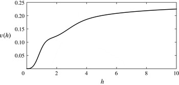
is the dimensionless dragging velocity due to the propagating Rayleigh SAW defined as
 $$\begin{eqnarray}\displaystyle v(h)\equiv \frac{1}{4h}\left(\frac{h\sinh (2h)-h\sin (2h)+2\cos (h)\cosh (h)}{\cos (2h)+\cosh (2h)}-1\right). & & \displaystyle\end{eqnarray}$$
It is easy to see that
 $v(0)=0$
and
 $v(h)\rightarrow 1/4$
as
 $h\rightarrow \infty$
(as shown in figure 2). We note that the expression (2.22) differs from the respective results obtained by Altshuler & Manor (Reference Altshuler and Manor2015) and Manor et al. (Reference Manor, Rezk, Friend and Yeo2015), since the perturbations of the liquid film thickness were not fully accounted for in these works.
Dimensionless dragging velocity due to the propagating Rayleigh SAW,
 $v(h)$
, as a function of the liquid film thickness
 $h$
.

We employ the hydrodynamic time scale defined in (2.19) as a unit of time and substitute the volume flux
 $Q$
into the mass conservation law, given from the integration of the continuity equation subject to the kinematic condition (2.10c
), to obtain the evolution equation for the liquid film thickness,
 $$\begin{eqnarray}\displaystyle h_{t}=-Q_{x}=-\left(hv(h)+\frac{1}{3We_{s}}h^{3}h_{xxx}\right)_{x}, & & \displaystyle\end{eqnarray}$$
where
 $We_{s}\equiv \unicode[STIX]{x1D712}ReCa/\unicode[STIX]{x1D716}^{3}$
is the scaled Weber number quantifying the ratio between the convective stress, imposed by the SAW, and the capillary stress, imposed by the surface tension at the free surface of the film.
Finally, we note that evolution equations visually similar to (2.23) were obtained previously, for instance by Shklyaev, Alabuzhev & Khenner (Reference Shklyaev, Alabuzhev and Khenner2009) who considered a liquid film on a vibrating substrate. However, in the case considered by by Shklyaev et al. (Reference Shklyaev, Alabuzhev and Khenner2009), the volume flux due to substrate vibration vanishes when the film is flat. The latter is not the case for the evolution equation (2.23), given here, due to the propagating nature of the SAW in this paper.
2.4 Thin-film equation in the steady state
Similarly to the Landau & Levich (Reference Landau and Levich1942) and the Bretherton (Reference Bretherton1961) models, we wish to show that the dragging of liquid by means of SAW can indeed result in a film of constant thickness. Not surprisingly, the latter corresponds to a static film profile, namely,
 $h_{t}=0$
. In this case one may integrate the evolution equation (2.23) over
 $x$
to obtain the equation governing the film thickness in a steady state,
 $$\begin{eqnarray}\displaystyle h_{xxx}=3We_{s}\frac{Q_{0}-hv(h)}{h^{3}}, & & \displaystyle\end{eqnarray}$$
where the integration constant
 $Q_{0}$
represents the steady volume flux throughout the film. In the case of
 $v(h)=1$
, equation (2.24) reduces to the well-known Landau–Levich equation (Landau & Levich Reference Landau and Levich1942). Indeed, Landau & Levich (Reference Landau and Levich1942) have investigated dragging of a liquid film by a plate moving with constant velocity. In our case, however, the dimensionless dragging velocity
 $v(h)$
depends on the film thickness
 $h$
. In § 3 we show that this new feature of (2.24) causes a qualitative change in the behaviour of the liquid film.
3 Steady states
In § 2 we have shown that the SAW excitation of a thin liquid film results in the transport of liquid in the direction of the propagating SAW. In this section we employ (2.24) to model the film profile in the overlap region connecting the static meniscus located upstream with the film of constant thickness
 $h_{\infty }$
downstream, as shown in figure 1.
In the case of dragging of a liquid film by a moving plate, it has been shown that the steady states characterized by monotonic behaviour of the film thickness, originally found by Landau & Levich (Reference Landau and Levich1942), correspond to the limit of perfectly wetting liquid in the absence of gravity (Snoeijer et al.
Reference Snoeijer, Ziegler, Andreotti, Fermigier and Eggers2008). Whereas for a partially wetting liquid in the presence of gravity, steady states with non-monotonic
 $h(x)$
exist (Snoeijer et al.
Reference Snoeijer, Ziegler, Andreotti, Fermigier and Eggers2008; Benilov et al.
Reference Benilov, Chapman, McLeod, Ockendon and Zubkov2010). In the present paper, the limit of the perfectly wetting liquid in the absence of gravity is considered.
Following Landau & Levich (Reference Landau and Levich1942), we match the film profile
 $h(x)$
with the static meniscus,
 $$\begin{eqnarray}\displaystyle h_{xx}\rightarrow 1\quad \text{as }x\rightarrow -\infty , & & \displaystyle\end{eqnarray}$$
and with the flat film,
 $$\begin{eqnarray}\displaystyle h_{x}\rightarrow 0,\quad h_{xx}\rightarrow 0\quad \text{as }x\rightarrow \infty . & & \displaystyle\end{eqnarray}$$
Boundary conditions (3.1)–(3.2) are applied at infinity, since the length scale of the overlap region of interest
 $L$
is small compared to the characteristic length of the meniscus
 $R$
and large compared to the typical thickness of the flat film
 $\unicode[STIX]{x1D6FF}$
,
 $$\begin{eqnarray}\displaystyle \unicode[STIX]{x1D6FF}\ll L\ll R. & & \displaystyle\end{eqnarray}$$
Furthermore, we argue that the contribution of the capillary forces to the volume flux
 $Q$
should vanish downstream, where the film is flat. The latter allows to express the volume flux in the steady state
 $Q_{0}$
in terms of a dimensionless thickness of the flat film,
 $h_{\infty }$
, as follows:
 $$\begin{eqnarray}\displaystyle Q_{0}=h_{\infty }v(h_{\infty }), & & \displaystyle\end{eqnarray}$$
where
 $h_{\infty }=\lim _{x\rightarrow +\infty }h$
.
We solve (2.24) subject to boundary conditions (3.1)–(3.2) by means of the shooting method. In particular, equation (2.24) is integrated using the MATLAB ordinary differential equations solver ode113. We start the integration from
 $x\rightarrow \infty$
, using trial values of
 $h$
for a given value of
 $We_{s}$
; then we use cubic splines, implemented in the MATLAB function spline, to interpolate the value of
 $h_{\infty }$
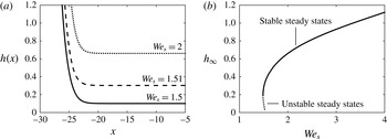
that satisfy the boundary condition (3.1). The calculated film profiles are shown in figure 3(a).
Profiles of the steady liquid film for various values of
 $We_{s}$
(a); and the dimensionless thickness of the resulting flat film,
 $h_{\infty }$
, versus
 $We_{s}$
(b).

We summarize the results of our numerical computations in the bifurcation diagram shown in figure 3(b). The bifurcation diagram reveals two important features of the system at hand.
-
(i) Steady solutions of the evolution equation (2.23) exist only for
 $We_{s}\gtrsim 1.49$
.
-
(ii) For
$We_{s}\gtrsim 1.49$
, there exist two branches of steady states meeting at
$We_{s}\approx 1.49$
. The latter hints that a saddle-node bifurcation occurs at
$We_{s}\approx 1.49$
, and thus, only one branch of the bifurcation diagram shown in figure 3(b) is stable. This conjecture is supported by the results of the stability analysis presented in § 4.2.


4 Time-dependent thin-film profiles
We proceed with the numerical analysis of the thin-film evolution equation (2.23).
4.1 Boundary conditions and method of solution
We are particularly interested in the evolution of the perturbations localized in the overlap region. Therefore, we approximate the boundary conditions in (3.1)–(3.2) as follows:
 $$\begin{eqnarray}\displaystyle h=h_{1},\quad h_{xx}=1\quad \text{at }x=x_{1}, & & \displaystyle\end{eqnarray}$$
 $$\begin{eqnarray}\displaystyle h=h_{2},\quad h_{x}=0\quad \text{at }x=x_{2}, & & \displaystyle\end{eqnarray}$$
where
 $h_{1}$
,
 $x_{1}$
,
 $h_{2}$
and
 $x_{2}$
are constants determined by the particular initial condition.
We solve (2.23) subject to boundary conditions (4.1) by means of the Newton–Kantorovich method (Boyd Reference Boyd2000). To ensure that the choice of the endpoints
 $x_{1}$
and
 $x_{2}$
does not affect the results, we used computational domains of different lengths, namely,
 $x_{2}-x_{1}=50$
and
 $100$
. All of the results presented below were obtained using the constant time step
 $\unicode[STIX]{x1D70F}=10^{-2}$
and the spatial discretization step
 $\unicode[STIX]{x1D6E5}=0.125$
. Similar results were also obtained at the finer resolution:
 $\unicode[STIX]{x1D70F}=2\times 10^{-3}$
and
 $\unicode[STIX]{x1D6E5}=0.05$
.
4.2 Stability of the steady states
Rigorous procedure of the linear stability analysis of the steady solutions of the evolution equation (2.23) is quite cumbersome. Instead, we demonstrate stability/instability of the steady states by means of direct numerical solution of (2.23). Specifically, we consider the evolution of the perturbed steady states defined as,
 $$\begin{eqnarray}\displaystyle \tilde{h}_{0}(x)=(1+a\text{e}^{-(x-x_{0})^{2}/b})h_{0}(x), & & \displaystyle\end{eqnarray}$$
where
 $h_{0}(x)$
is a solution of (2.24) with boundary conditions (3.1)–(3.2),
 $a$
is the perturbation amplitude,
 $b$
is the width of the perturbation and
 $x_{0}$
is the position of the centre of the perturbation. Naturally, we expect the perturbations of stable steady states to decay, whereas the perturbations of unstable steady states are expected to grow. To detect decay or growth of the perturbations, we employ the
 $L_{1}$
norm of the difference between the current film profile
 $h(x,t)$
and the steady state
 $h_{0}(x)$
, namely,
 $$\begin{eqnarray}\displaystyle \Vert h(x,t)-h_{0}(x)\Vert \equiv \int _{x_{1}}^{x_{2}}|h(x,t)-h_{0}(x)|\,\text{d}x. & & \displaystyle\end{eqnarray}$$
We study the stability of the steady states obtained at
 $We_{s}=$
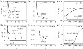
1.49, 1.5, 1.52 and 2. Typical results of the numerical computations are shown in figure 4. Overall, we observe that the perturbations of the steady states with
 $h_{\infty }>0.19$
lead to a steady state in the vicinity of
 $h_{0}(x)$
(the latter is not reproduced exactly due to numerical inaccuracies in the estimations of
 $h_{1}$
and
 $h_{2}$
). In turn, steady states with
 $h_{\infty }<0.19$
break down due to perturbations: when the perturbation is a deep trough, i.e. for
 $a\lesssim -0.1$
, gradual thinning of the film is observed (as shown in figure 4
a); while for
 $a>-0.1$
our computations result in redeposition of the film with the thickness corresponding to a stable steady state (the latter case is illustrated in figure 4
d).
The observations summarized in the paragraph above support our conjecture that a branch of stable steady states, for
 $h_{\infty }>0.19$
, meets a branch of unstable steady states, for
 $h_{\infty }<0.19$
, at a saddle-node bifurcation point, where
 $We_{s}\approx 1.49$
, as shown in figure 3(b).
Three types of the dynamical behaviour observed in the course of the numerical analysis of the thin-film evolution equation in (2.23): gradual thinning of an unstable film observed for
 $h_{\infty }=0.101$
and
 $a=-0.1$
is shown on (a); redeposition of the film observed for
 $h_{\infty }=0.101$
and
 $a=0.1$
is shown on (d); stable films observed for
 $h_{\infty }=0.276$
and
 $a=-0.1,\;0.01$
are shown in (b,e). The evolution of the distance from the initial condition measured using (4.3) is shown in (c,f). The results presented in this figure were obtained for
 $We_{s}=1.5$
,
 $b=10$
,
 $x_{0}=-20$
,
 $x_{2}-x_{1}=50$
,
 $\unicode[STIX]{x1D70F}=2\times 10^{-3}$
and
 $\unicode[STIX]{x1D6E5}=0.05$
. Note that the particular values of
 $h_{\infty }$
in the figures are obtained from the solution of (2.24) and rounded to 3 significant figures.

4.3 Decay of the thin film in the absence of steady states
We finalize the analysis of the thin-film evolution equation (2.23) with a discussion on the film dynamics in the absence of steady states, namely, in the case of
 $We_{s}<1.49$
. In this case, we employ one of the stable steady states obtained in § 3 for
 $We_{s}\gtrsim 1.49$
as an initial condition, and study its evolution by means of numerical solution of (2.23).
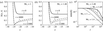
Our numerical computations for
 $We_{s}=1$
, 1.4, 1.45 and 1.48 result in the gradual thinning of the liquid film (as shown in figure 5). We observe that the thinning is a two-stage process: during the first stage the minimal film thickness remains almost constant, whereas during the second stage the decay of the minimal film thickness is close to exponential (as shown in figure 5
c). Moreover, higher values of
 $We_{s}$
correspond to a longer first stage and a higher rate of decay in the second stage. That is, unlike in the case where surface tension is the only driving force of the film dynamics (Wong, Fatt & Radke Reference Wong, Fatt and Radke1996), in the presence of SAW the decay of the film thickness in time is not exponential. It is also worth noting that in the course of thinning the liquid film attains a dimple-like shape, which is typical to models that neglect the effects of a disjoining pressure between the solid and the film interfaces (Chan, Klaseboer & Manica Reference Chan, Klaseboer and Manica2011).
Decay of the thin-film profile in the absence of steady states observed for
 $x_{2}-x_{1}=50$
,
 $\unicode[STIX]{x1D70F}=2\times 10^{-3}$
,
 $\unicode[STIX]{x1D6E5}=0.05$
and several values of
 $We_{s}$
. Thin-film profiles for
 $We_{s}=1$
are shown in (a); film profiles for
 $We_{s}=1.48$
are shown in (b); evolution of the minimal film thickness in the course of our computations for
 $We_{s}=1$
, 1.4, 1.45 and 1.48 is shown in (c).

5 Discussion
In this paper we use theory to investigate the dragging of a thin liquid film from a static meniscus using a Rayleigh SAW, propagating in the solid substrate, as shown in figure 1. We employ the lubrication approximation to derive a thin-film evolution equation (2.23), governing the dynamics of the thickness of the film
 $h(x,t)$
. We show that in a steady state the thickness of the film is governed by a generalized Landau–Levich equation (2.24) with the dragging velocity of the film depending on its thickness. We demonstrate that this new feature of the model causes a qualitative change in the predicted thin-film behaviour.
Unlike the Landau–Levich equation, equation (2.24) matches a static meniscus with a flat film only for sufficiently large values of the scaled Weber number, namely,
 $We_{s}\gtrsim 1.49$
. Moreover, for
 $We_{s}\gtrsim 1.49$
, equation (2.24) possesses two branches of solutions (as shown in figure 3
b). The numerical solution of the evolution equation (2.23) with the boundary conditions (4.1) suggests that stable steady states belong to the top branch of the bifurcation diagram in figure 3(b), whereas the steady states corresponding to the bottom branch of the diagram are unstable. The latter implies that
 $We_{s}\approx 1.49$
is a saddle-node bifurcation point.
Further, by means of a numerical solution of (2.23) with the boundary conditions (4.1) we demonstrate that in the absence of steady states, i.e. for
 $We_{s}<1.49$
, the liquid film thins gradually. In the absence of SAW it is possible to obtain the universal rate of film thinning (Wong et al.
Reference Wong, Fatt and Radke1996). However, in our case the rate of decay depends on the scaled Weber number. We also note that in the course of the thinning the film attains a dimple-like shape typical to models that neglect the effects of a disjoining pressure between the solid and the interfaces of the film (Chan et al.
Reference Chan, Klaseboer and Manica2011).
Finally, we note that in the present paper we consider the limit of perfectly wetting liquid in the absence of gravity. It has been shown that for a partially wetting liquid in the presence of gravity, the steady states with non-monotonic behaviour of
 $h(x)$
exist (Snoeijer et al.
Reference Snoeijer, Ziegler, Andreotti, Fermigier and Eggers2008; Benilov et al.
Reference Benilov, Chapman, McLeod, Ockendon and Zubkov2010). The question of the existence of non-monotonic steady states of (2.23) is left for future research.
Acknowledgement
We acknowledge support of this research by the Israel Science Foundation (ISF) under grant no. 489/14.
Appendix A. Acoustic radiation pressure
The assumption of a constant radius of curvature
 $R$
implies that the acoustic radiation pressure,
 $P_{ar}$
, exerted on the meniscus by sound waves leaking off the propagating SAW and impinging on the free surface of the liquid, is negligible compared to the Laplace pressure in the liquid,
 $P_{L}$
, due to curvature of the meniscus, i.e.
 $$\begin{eqnarray}\displaystyle P_{L}\gg P_{ar}. & & \displaystyle\end{eqnarray}$$
The acoustic radiation pressure on the free surface of the liquid due to the impinging of a sound wave, propagating in the liquid in a direction perpendicular to the free surface and with a velocity amplitude
 $U$
, can be estimated as follows (Beyer Reference Beyer1974; Lee & Wang Reference Lee and Wang1993),
 $$\begin{eqnarray}\displaystyle P_{ar}=\frac{\unicode[STIX]{x1D70C}U^{2}}{2}\left(1+\frac{B}{2A}\right). & & \displaystyle\end{eqnarray}$$
We note that when a sound wave leaks off the SAW in the solid, the velocity amplitude of the sound wave is the same as the normal component of the velocity amplitude of the solid surface (
 $U$
). As the sound wave propagates in the liquid away from the solid it will attenuate due to viscous and thermal mechanisms. Using the definition of the Laplace pressure and (A 2), the condition (A 1) can be rewritten as follows,
 $$\begin{eqnarray}\displaystyle R\ll \frac{2\unicode[STIX]{x1D6FE}}{\unicode[STIX]{x1D70C}U^{2}}\left(1+\frac{B}{2A}\right)^{-1}, & & \displaystyle\end{eqnarray}$$
where
 $\unicode[STIX]{x1D6FE}$
is the surface tension of the liquid.
Appendix B. Asymptotic representation of the SAW
We consider a Rayleigh SAW, propagating in a half-space of an isotropic solid along the
 $x$
-coordinate and supporting in-plane,
 $X(x,y,t)$
, (along the solid surface) and out-of-plane,
 $Y(x,y,t)$
, (transverse to the solid surface) displacements in the solid, shown in figure 1. In the limit of small displacements the ratio between the characteristic magnitude of the displacements,
 $U/\unicode[STIX]{x1D714}$
, and the length scale of the SAW in the solid along the
 $x$
and
 $y$
coordinates,
 $k^{-1}$
, is small, such that
 $\unicode[STIX]{x1D701}\equiv (U/\unicode[STIX]{x1D714})/k^{-1}\ll 1$
; the quantities
 $U$
,
 $\unicode[STIX]{x1D714}$
and
 $k$
are the characteristic velocity of the displacements, the angular frequency and the wavenumber of the SAW, respectively. The transformations
 $(X,Y)\rightarrow (U/\unicode[STIX]{x1D714})(\tilde{X},{\tilde{Y}}),~(x,y)\rightarrow k^{-1}(\tilde{x},{\tilde{y}})$
and
 $t\rightarrow \unicode[STIX]{x1D714}^{-1}\tilde{t}$
give the scaled displacement field in the solid that may be described as an asymptotic series (Spencer Reference Spencer1970; Parker Reference Parker1988) in
 $\unicode[STIX]{x1D701}$
, such that,
 $$\begin{eqnarray}\displaystyle (\tilde{X},{\tilde{Y}})=\unicode[STIX]{x1D701}(\tilde{X}_{1},{\tilde{Y}}_{1})+\unicode[STIX]{x1D701}^{2}(\tilde{X}_{2},{\tilde{Y}}_{2})+\cdots \,, & & \displaystyle\end{eqnarray}$$
where the non-dimensional functions
 $\tilde{X}_{1},~\tilde{X}_{2},~{\tilde{Y}}_{1},~{\tilde{Y}}_{2}$
, etc. are
 $O(1)$
functions. The leading-order terms in the asymptotic expansion is associated with the theory of linear elasticity. Terms of lower magnitudes in the series correct the displacement field for nonlinearities in the governing equations that are associated with the nonlinear stress components, the displacements in the solid, etc.
The velocity field in the solid may then be represented by
 $$\begin{eqnarray}\displaystyle (\tilde{X}_{\tilde{t}},{\tilde{Y}}_{\tilde{t}})=\unicode[STIX]{x1D701}(\tilde{X}_{1,\tilde{t}},{\tilde{Y}}_{1,\tilde{t}})+\unicode[STIX]{x1D701}^{2}(\tilde{X}_{2,\tilde{t}},{\tilde{Y}}_{2,\tilde{t}})+\cdots \,. & & \displaystyle\end{eqnarray}$$
Further, the velocity field at the solid surface is given by
 $(\tilde{X}_{\tilde{t}},{\tilde{Y}}_{\tilde{t}})|_{{\tilde{y}}={\tilde{Y}}}$
; the solid surface satisfies the condition
 ${\tilde{y}}-{\tilde{Y}}=0$
. Expanding the expression for the surface velocity near the position of the solid surface at rest,
 $y=0$
, gives
 $$\begin{eqnarray}\displaystyle (\tilde{X}_{\tilde{t}},{\tilde{Y}}_{\tilde{t}})|_{{\tilde{y}}={\tilde{Y}}}=\unicode[STIX]{x1D701}(\tilde{X}_{1,\tilde{t}},{\tilde{Y}}_{1,\tilde{t}})|_{{\tilde{y}}=0}+O(\unicode[STIX]{x1D701}^{2}). & & \displaystyle\end{eqnarray}$$
In dimensional terms the velocity at the solid surface is given by
 $$\begin{eqnarray}\displaystyle (X_{t},Y_{t})|_{y=Y(y=0)}=(X_{1,t},Y_{1,t})|_{y=0}+O(U\unicode[STIX]{x1D701}), & & \displaystyle\end{eqnarray}$$
and the first term of the expansion on the right-hand side of the equation is exactly the result given from the theory of linear elasticity in an isotropic solid for an infinitesimally small displacement in the solid (Wilmanski & Albers Reference Wilmanski and Albers2014), i.e.
 $$\begin{eqnarray}\displaystyle (X_{1,t},Y_{1,t})|_{y=0}=U[\cos (\unicode[STIX]{x1D714}t-kx),\unicode[STIX]{x1D712}\sin (\unicode[STIX]{x1D714}t-kx)]. & & \displaystyle\end{eqnarray}$$