1. Introduction
Chaotic mixing of a passive scalar, such as temperature or pollutant concentration, by a turbulent velocity field, is often observed to create convoluted spatial structures, characterized by elongated lamellar (in two dimensions) or sheets (in three dimensions) with a wide range of self-similar scales, which produce large intermittent fluctuations with a non-Gaussian probability density function (p.d.f.) (Ottino Reference Ottino1989; Sreenivasan, Ramshankar & Meneveau Reference Sreenivasan, Ramshankar and Meneveau1989; Procaccia et al. Reference Procaccia, Ching, Constantin, Kadanoff, Libchaber and Wu1991; Villermaux Reference Villermaux2012). The strong non-Gaussian fluctuations in turbulent mixing are relevant to the transport of heat and mass in many natural systems of geophysical and astrophysical scales, such as in the ocean (Rahmstorf Reference Rahmstorf2000), the atmosphere (Sidorenkov Reference Sidorenkov2009) and the outer layer of the Sun (Cattaneo, Emonet & Weiss Reference Cattaneo, Emonet and Weiss2003), and in numerous industrial processes of polymers, minerals, fine chemicals, paints, cosmetics, food, water and waste-water treatment (Ottino Reference Ottino1989; Paul, Atiemo-Obeng & Kresta Reference Paul, Atiemo-Obeng and Kresta2004; Dimotakis Reference Dimotakis2005).
Experimentally or numerically well-controlled studies of turbulent temperature fluctuations are often conducted in Rayleigh–Bénard convection (or RBC), which occurs in a confined fluid layer between two horizontal plates heated from below and cooled from above. The convective flow in RBC is determined by the Rayleigh number, a dimensionless form of buoyancy,  ${\textit {Ra}} \equiv \psi g \Delta T\, H^3/(\nu \kappa )$ and the Prandtl number
 ${\textit {Pr}} \equiv \nu /\kappa$. Here
 $g$ is the gravitational acceleration,
 $\Delta T$ is the temperature difference across the fluid layer of height
 $H$, and
 $\psi$,
 $\nu$ and
 $\kappa$ are, respectively, the thermal expansion coefficient, and the viscous and thermal diffusivities of the convecting fluid. For a detailed review of RBC turbulence, please see Siggia (Reference Siggia1994), Kadanoff (Reference Kadanoff2001), Ahlers, Grossmann & Lohse (Reference Ahlers, Grossmann and Lohse2009), Lohse & Xia (Reference Lohse and Xia2010), Chillá & Schumacher (Reference Chillá and Schumacher2012) and references therein.
When the Rayleigh number is sufficiently large (e.g.  ${\textit {Ra}} \gtrsim 10^8$ for
 ${\textit {Pr}}\simeq 4.4$), the bulk fluid becomes turbulent and a large-scale circulation (LSC) is formed across the convection cell (Krishnamurti & Howard Reference Krishnamurti and Howard1981; Zocchi, Moses & Libchaber Reference Zocchi, Moses and Libchaber1990). The LSC is driven by the warm and cold plumes emitted from the unstable thermal boundary layers (BLs) near the bottom and top conducting plates and is maintained in a turbulent environment. This large-scale flow with
 ${\textit {Pr}}>1$ has been studied extensively in upright cylindrical cells of aspect ratio unity (Du & Tong Reference Du and Tong2000; Qiu & Tong Reference Qiu and Tong2001; Xi, Lam & Xia Reference Xi, Lam and Xia2004; Sun, Xia & Tong Reference Sun, Xia and Tong2005), in which the LSC has a single roll structure, with its size comparable to the cell height. An intriguing feature of this convective flow is the continuing appearance of large fluctuations in the temperature field, which do not follow the Gaussian statistics (Kadanoff Reference Kadanoff2001). The measured p.d.f.
 $P(\delta T)$ of temperature fluctuations
 $\delta T$ from the mean value in the central region of the cell has a long exponential tail with its amplitude varied by more than four decades, which falls off much slower than a Gaussian (Castaing et al. Reference Castaing, Gunaratne, Heslot, Kadanoff, Libchaber, Thomae, Wu, Zaleski and Zanetti1989; Sano, Wu & Libchaber Reference Sano, Wu and Libchaber1989; Gollub et al. Reference Gollub, Clarke, Gharib, Lane and Mesquita1991; Belmonte, Tilgner & Libchaber Reference Belmonte, Tilgner and Libchaber1994; Niemela et al. Reference Niemela, Skrbek, Sreenivasan and Donnelly2000; Du & Tong Reference Du and Tong2001; Zhou & Xia Reference Zhou and Xia2002; He, Tong & Xia Reference He, Tong and Xia2007; Wei & Ahlers Reference Wei and Ahlers2016).
In a recent experiment, He, Wang & Tong (Reference He, Wang and Tong2018) showed that the exponential temperature p.d.f. in RBC is generated by the thermal plumes, which intermittently emit from the thermal boundary layers (BLs) and carry temperature fluctuations from the BLs to the bulk region of the flow (Kadanoff Reference Kadanoff2001; Siggia Reference Siggia1994). Because of the rapid mixing and advection of warm and cold plumes passing through the central region of the convection cell, the local thermal dissipation rate  $\epsilon (t) \equiv \kappa [{\nabla } T(t)]^2$ associated with the thermal plumes was found to have a broad distribution
 $f(\epsilon )$ (He et al. Reference He, Tong and Xia2007; He & Tong Reference He and Tong2009). Consequently, the temperature p.d.f.
 $P(\delta T)$ can be written as
 \begin{equation} P(\delta T) = \int_{0}^{\infty}f(\epsilon)\,G(\delta T\vert \epsilon)\,{\rm d}\epsilon, \end{equation}
where  $G(\delta T\vert \epsilon )$ is the conditional p.d.f. of temperature fluctuations when
 $\epsilon$ is held constant (He et al. Reference He, Wang and Tong2018). The measured
 $G(\delta T \vert \epsilon )$ was found to be of Gaussian form
 \begin{equation} G(\delta T\vert \epsilon) = \frac{1}{\sqrt{2{\rm \pi}}\sigma_0(\epsilon)} \exp({-\delta T^2/[2\sigma_0^2(\epsilon)]}), \end{equation}
and its variance  $\sigma ^2_0$ for different values of
 $\epsilon$ follows an exponential distribution
 \begin{equation} F(\sigma_0^2) = \frac{1}{\sigma_T^2}\exp({-\sigma_0^2/\sigma_T^2}), \end{equation}
where  $\sigma _T$ is the r.m.s. value of the measured
 $\delta T$. The convolution of the two distribution functions gives rise to the exponential p.d.f.
 $P(\delta T)$. The physical origin of (1.2) and (1.3) was discussed in He et al. (Reference He, Wang and Tong2018).
With this finding, Wang, He & Tong (Reference Wang, He and Tong2019) further proposed that the temperature p.d.f.  $P(\delta T)$ at other (non-symmetric) locations of the cell can be obtained by assuming the overall temperature fluctuations result from two independent sources, namely,
 \begin{equation} \delta T(t)=\delta T_B(t)+\delta T_P(t), \end{equation}
where  $\delta T_B(t)$ denotes temperature fluctuations from the (turbulent) background with a Gaussian distribution, and
 $\delta T_P(t)$ represents those resulting from the thermal plumes with an exponential distribution. With (1.4), the temperature p.d.f.
 $P(\delta T)$ can be derived from a convolution of the two fluctuation modes with a relative ratio between the two modes and a duty-cycle parameter for plume intermittency. These two adjustable parameters were used to fit the measured
 $P(\delta T)$ in different flow regions along the central vertical axis of two different convection cells. A good agreement between the calculated
 $P(\delta T)$ and the experimental results was obtained (Wang et al. Reference Wang, He and Tong2019), which suggests that the above theoretical framework captures the essential physics behind the non-Gaussian statistics of temperature fluctuations in a closed convection cell.
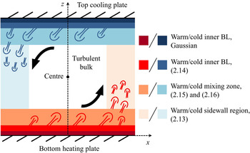
Based on the spatial distribution of thermal plumes in the closed convection cell, the convective flow can be divided into five distinct regions, namely, thermal BL, mixing zone, turbulent bulk, sidewall and cell centre, as shown in figure 1. Thermal plumes first form and grow in the outer BL and they are mixed and bundled together in the mixing zone. Because of the coherent LSC, most of the thermal plumes in the mixing zone are eventually swept to the sidewall region. As a result, the bulk region has fewer plumes. The mixing zone can be further divided into an inner region ( $0.04 \lesssim z/H \lesssim 0.1$) and an outer region (
 $0.1 \lesssim z/H \lesssim 0.3$), depending on whether the thermal plumes emitted from the opposite BL can be detected (outer mixing zone) or not (inner mixing zone).
Sketch of distinct flow regions in the  $A = 1$ upright cylinder: inner BL (
 $z/\delta \lesssim 0.6$), outer BL (
 $0.6 \lesssim z/\delta \lesssim 4$), mixing zone (
 $0.04 \lesssim z/H \lesssim 0.3$), turbulent bulk (
 $0.3 \lesssim z/H \lesssim 0.5$ and
 $|x|/D_{{up}} \lesssim 0.3$), sidewall region (
 $0.3 \lesssim |x|/D_{{up}} \lesssim 0.5$) and cell centre (
 $z/H=0.5$). Here
 $\delta$ is the thermal BL thickness and
 $A \equiv D_{{up}}/H$ is the aspect ratio of the cylindrical cell with diameter
 $D_{{up}}$ and height
 $H$. The dashed lines show the Cartesian coordinates used in the experiment. The black arrows indicate the direction of the large-scale circulation. The temperature p.d.f.s in each flow region are described by the given equations.

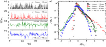
Figure 2 shows the evolution of local temperature fluctuations  $\delta {T}(t)$ and their p.d.f.s in four different flow regions. The measured
 $\delta {T}(t)$ in the outer BL (figure 2a) exhibits dense positive spikes, indicating that warm plumes are formed intermittently in this region. These intermittent temperature spikes give rise to a downward-bending tail in the temperature p.d.f.
 $P(\delta T)$ (black squares in figure 2(e) with
 $\delta {T}/\sigma _T\gtrsim 1$). Furthermore, the measured
 $\delta {T}(t)$ has a continuous background of small-amplitude fluctuations resulting from thermal conduction. These continuous fluctuations produce a symmetric distribution in the resulting
 $P(\delta T)$ (black squares in figure 2(e) with
 $\delta {T}/\sigma _T < 1$). In the inner mixing zone (figure 2b), only those positive spikes with a large amplitude remain in the measured
 $\delta {T}(t)$, but their number is reduced considerably because many warm plumes have been swept to the sidewall region by the LSC. As a result, continuous small-amplitude fluctuations from the turbulent background occupy a longer duration of time in the measured
 $\delta {T}(t)$, and the resulting
 $P(\delta T)$ exhibits an exponential-like long tail (red circles in figure 2(e) with
 $\delta {T}/\sigma _T\gtrsim 1.5$). At the cell centre (figure 2c), temperature fluctuations are symmetric because of the reflection symmetry between the upper and lower halves of the convection cell. The resulting
 $P(\delta T)$ thus has two symmetric exponential tails on both sides of the temperature p.d.f. (green up-pointing triangles in figure 2e). Finally, in the sidewall region (figure 2d), the measured
 $\delta {T}(t)$ exhibits many positive spikes resulting from the rising warm plumes in the region and a few negative spikes from the falling cold plumes. The resulting
 $P(\delta T)$ in the sidewall region possesses a most complex form (blue down-pointing triangles in figure 2e).
Measured time series of local temperature fluctuations  $\delta {T}(t)$ in four different flow regions: (a) outer BL (
 $x=0$ mm and
 $z=1.6$ mm), (b) inner mixing zone (
 $x=0$ mm and
 $z=9.5$ mm), (c) cell centre (
 $x=0$ mm and
 $z=95$ mm) and (d) sidewall region (
 $x=85$ mm and
 $z=95$ mm). In the plot,
 $\delta {T}(t)$ is normalized by its r.m.s. value
 $\sigma _T$. The measurements are made in the upright cylinder filled with water and at
 ${\textit {Ra}}=4.4\times 10^9$ and
 ${\textit {Pr}}=4.4$ for (a–c) and
 ${\textit {Ra}}=4.7\times 10^9$ and
 ${\textit {Pr}}=5.4$ for (d). The coordinate system used is shown in figure 3(b). (e) Corresponding p.d.f.s of the measured
 $\delta {T}/\sigma _T$.

The complex spatial distribution of thermal plumes gives rise to a rich behaviour of the temperature p.d.f. Nonetheless, we found that the simple decomposition of temperature fluctuations  $\delta T(t)$ into a Gaussian background together with a contribution from individual plumes (one plume at a time as recorded by a temperature sensor), as shown in (1.4), works for most of the regions, as shown in figure 1. Hereafter, we refer to these regions collectively as the ‘single-plume’ region. However, we find two exceptional regions in the closed convection cell, in which the plumes are highly concentrated and the above mentioned ‘single-plume’ decomposition of
 $\delta T(t)$ does not work. These two regions are the sidewall and outer BL regions, in which the thermal plumes merge together in space and produce large temperature fluctuations. This ‘multi-plume’ effect changes the tail part of the temperature p.d.f.
 $P(\delta T)$ (see figure 2e), causing it to deviate from the functional form derived from (1.4).
In this paper, we take the multi-plume effect into account and further decompose  $\delta T_P(t)$ into two independent and mutually excluded fluctuation modes, namely,
 $\delta T_P(t)=\{\delta T_{s}(t), \delta T_{m}(t)\}$, where
 $\delta T_{s}(t)$ and
 $\delta T_{m}(t)$ are, respectively, temperature fluctuations produced by single and multiple plumes. By assuming that the p.d.f. of
 $\delta T_{m}(t)$ follows the Gamma distribution, and together with the given p.d.f. form of the other two independent sources, we derive an analytical form of
 $P(\delta T)$, which is a sum of convolutions of p.d.f.s of individual fluctuation modes and contains a set of spatially varying parameters that account for the relative strength and incidence of each fluctuation mode, and the average number of thermal plumes involved in the multi-plume effect. A good agreement between the calculated and measured
 $P(\delta T)$ is obtained with the temperature data collected at various locations in two different convection cells. Our results demonstrate that the theoretical framework proposed by Wang et al. (Reference Wang, He and Tong2019) with the multi-plume effect included is capable of explaining the complex non-Gaussian form of temperature p.d.f.s in a highly non-uniform convective flow with a unified set of physical parameters.
The remainder of the paper is organized as follows. We first derive a general form of temperature p.d.f.  $P(\delta T)$ for turbulent thermal convection in § 2. In § 3, we briefly describe the two convection cells and experimental methods used for temperature data acquisition in turbulent RBC. In § 4, we present the measured p.d.f.s
 $P(\delta T)$ along the central axis of the cell and in the sidewall region at the mid-height of the convection cell, and compare the experimental results with the theoretical model. Finally, we conclude the paper with a summary in § 5.
2. Update of the theoretical framework
We now expand the theory of Wang et al. (Reference Wang, He and Tong2019) by assuming that the plume-induced temperature fluctuations  $\delta T_P$ in (1.4) contain contributions from both single and multiple plumes, namely,
 \begin{equation} \delta T_P(t)=\left\{\delta T_{sw}(t), \delta T_{mw}(t), \delta T_{sc}(t), \delta T_{mc}(t)\right\}, \end{equation}
where the subscripts ‘ $sw$’ and ‘
 $sc$’ denote, respectively, the single-warm and single-cold plumes, and the subscripts ‘
 $mw$’ and ‘
 $mc$’ denote, respectively, the multiple-warm and multiple-cold plumes. As shown in Wang et al. (Reference Wang, He and Tong2019), the continuous background temperature fluctuations
 $\delta T_B(t)$ follow the Gaussian distribution with zero mean and r.m.s. value
 $\sigma _B$:
 \begin{equation} P_B(\delta T_B)=\frac{1}{\sqrt{2{\rm \pi}}\sigma_B} \exp({-\delta T^2_B/(2\sigma_B^2)}), \quad \delta T_B\in(-\infty, +\infty) . \end{equation}
As shown in He et al. (Reference He, Wang and Tong2018), temperature fluctuations from single plumes have a simple exponential p.d.f.
 \begin{equation} P_{sw}(\delta T_{sw})=\frac{1}{\sigma_w} \exp({-\delta T_{sw}/\sigma_w}), \quad \delta T_{sw}\in[0, +\infty) \ \end{equation}
for  $\delta T_{sw}(t)$ and
 \begin{equation} P_{sc}(\delta T_{sc})=\frac{1}{\sigma_c} \exp({\delta T_{sc}/\sigma_c}), \quad \delta T_{sc}\in(-\infty,0], \end{equation}
for  $\delta T_{sc}(t)$. Here
 $\sigma _w$ and
 $\sigma _c$ are the r.m.s. values of
 $\delta T_{sw}(t)$ and
 $\delta T_{sc}(t)$, respectively. The condition
 $\delta T_{sw}\geq 0$ (
 $\delta T_{sc}\leq 0$) applies for warm (cold) plumes, and states that the thermal plumes are moving fluid parcels with their temperature fluctuations larger (smaller) than the average background temperature.
The single-plume mode described in (2.3) and (2.4) was found to be a dominant one in most regions along the central axis of the convection cell (Wang et al. Reference Wang, He and Tong2019). Nonetheless, we find that multi-plume clusters appear frequently in the outer BL region and in the sidewall region, which is an extra effect to be considered in addition to the single-plume mode. When a warm plume cluster contains  $n$ independent warm plumes, its temperature fluctuation is a sum of
 $n$ independent ones, namely,
 \begin{equation} \delta T_{mw}(t) = \delta T_{sw,1}(t)+\delta T_{sw,2}(t)+\cdots+\delta T_{sw,n}(t), \end{equation}
where each term results from single warm plumes at the measuring location. All the p.d.f.s of  $\delta T_{sw,i}(t)$ with
 $i = 1,\ldots, n$ obey the same exponential distribution, as shown in (2.3). As a result, the p.d.f. of their sum
 $\delta T_{mw}(t)$ follows the gamma distribution:
 \begin{equation} P_{mw}(\delta T_{mw})=\frac{\delta T_{mw}^{n_w-1} \exp({-\delta T_{mw}/\sigma_w})}{\varGamma(n_w)\,\sigma_w^{n_w}} , \quad \delta T_{mw}\in[0, +\infty) . \end{equation}
Similarly, the p.d.f. of  $\delta T_{mc}(t)$ from multiple-cold plumes is
 \begin{equation} P_{mc}(\delta T_{mc})=\frac{\left(-\delta T_{mc}\right)^{n_c-1} \exp({\delta T_{mc}/\sigma_c})}{\varGamma(n_c)\,\sigma_c^{n_c}}, \quad \delta T_{mc}\in(-\infty,0] . \end{equation}
The gamma distribution is used to model the distribution of a random variable that is a sum of  $n$ independent and identically distributed random variables following an exponential distribution with rate parameter
 $1/\sigma$ (Hogg & Craig Reference Hogg and Craig1978). It has been used in a variety of applications ranging from describing the size of insurance claims (Boland Reference Boland2007) and the amount of rainfall (Aksoy Reference Aksoy2000) to the protein concentration in live cells (Friedman, Cai & Xie Reference Friedman, Cai and Xie2006). It has also been used previously to describe concentration fluctuations of a dye in a turbulent jet (Villermaux & Duplat Reference Villermaux and Duplat2003; Duplat & Villermaux Reference Duplat and Villermaux2008; Le Borgne et al. Reference Le Borgne, Huck, Dentz and Villermaux2017). When
 $n_w = 1$ (or
 $n_c = 1$), the gamma distribution becomes the simple exponential distribution for single plumes. For
 $n_w>1$ (or
 $n_c>1$), the gamma distribution is a single-peaked function with a value of zero at the origin. It has larger effects on the distribution of large fluctuations. In principle, one needs a separate gamma distribution for each given type of multi-plume clusters of size
 $n$, and the total distribution would be a sum of gamma distributions with
 $n = 1, 2, 3, \ldots, N$. The experimental results to be discussed below reveal that the thermal plumes often organize themselves into two groups. One group is the individual single plumes with
 $n =1$, and the other group is the multi-plume clusters with a narrow size distribution so that a single gamma distribution is adequate to describe their effect on
 $P(\delta T)$. In this case, the value of
 $n_w$ (
 $n_c$) becomes a positive real number representing the average number of warm (cold) plumes in the multi-plume clusters at the measuring location.
Because the emission and appearance of thermal plumes at the measuring location is intermittent, the four plume fluctuation modes,  $\delta T_{sw}(t)$,
 $\delta T_{mw}(t)$,
 $\delta T_{sc}(t)$ and
 $\delta T_{mc}(t)$, do not occur continuously. To characterize this intermittency effect, we introduce four duty-cycle parameters,
 $\beta _{sw}$,
 $\beta _{sc}$,
 $\beta _{mw}$ and
 $\beta _{mc}$, each varying from 0 to 1, to describe the incidence of these fluctuation modes. As
 $\delta T_{sw}(t)$ and
 $\delta T_{mw}(t)$ (or
 $\delta T_{sc}(t)$ and
 $\delta T_{mc}(t)$) are mutually exclusive at the measuring point (otherwise, they would be referred to as a new multi-plume cluster), their coincidence is thus zero. When there are only warm plumes present at the measuring location, the incidence of detecting the background fluctuation
 $\delta T_B(t)$ is
 $(1-\beta _{sw}-\beta _{mw})$. Similarly, when there are only cold plumes present at the measuring location, the incident of detecting
 $\delta T_B(t)$ is
 $(1-\beta _{sc}-\beta _{mc})$. When both warm and cold plumes are present at the measuring location and they are independent of each other, one has
 $\beta _{sw} + \beta _{mw} \leq 1$ and
 $\beta _{sc} + \beta _{mc} \leq 1$. In this case, the total temperature fluctuations
 $\delta T(t)$ can be expressed as
 \begin{align} \delta T(t)=\left\{
\begin{array}{@{}ccc@{}} \delta T_B(t), & \delta T_B(t)+\delta
T_{sc}(t), & \delta T_B(t)+\delta T_{mc}(t)\\ \delta
T_B(t)+\delta T_{sw}(t), & \delta T_B(t)+\delta
T_{sw}(t)+\delta T_{sc}(t), & \delta T_B(t)+\delta
T_{sw}(t)+\delta T_{mc}(t)\\ \delta T_B(t)+\delta
T_{mw}(t), & \delta T_B(t)+\delta T_{mw}(t)+\delta
T_{sc}(t), & \delta T_B(t)+\delta T_{mw}(t)+\delta
T_{mc}(t) \end{array} \right\},
\end{align}
and the corresponding incidence is given by
 \begin{align} \left\{
\begin{array}{@{}ccc@{}}
(1-\beta_{sw}-\beta_{mw})(1-\beta_{sc}-\beta_{mc}), &
\beta_{sc}(1-\beta_{sw}-\beta_{mw}), &
\beta_{mc}(1-\beta_{sw}-\beta_{mw})\\
\beta_{sw}(1-\beta_{sc}-\beta_{mc}), &
\beta_{sw}\beta_{sc}, & \beta_{sw}\beta_{mc}\\
\beta_{mw}(1-\beta_{sc}-\beta_{mc}), &
\beta_{mw}\beta_{sc}, & \beta_{mw}\beta_{mc}
\end{array} \right\}. \end{align}
From the above discussions, we obtain the p.d.f.  $P(\delta T)$ as a weighted sum of convolutions of the p.d.f.s for individual fluctuation modes:
 \begin{align} P(\delta T) &=
(1-\beta_{sw}-\beta_{mw})(1-\beta_{sc}-\beta_{mc})\,P_B(\delta{T})\nonumber\\
&\quad
+\beta_{sw}(1-\beta_{sc}-\beta_{mc})\int_{0}^{+\infty}P_B(\delta
T-\delta T_{sw})\,P_{sw}(\delta T_{sw})\,\mathrm{d}(\delta
T_{sw})\nonumber\\ &\quad
+\beta_{mw}(1-\beta_{sc}-\beta_{mc})\int_{0}^{+\infty}P_B(\delta
T-\delta T_{mw})\,P_{mw}(\delta T_{mw})\,\mathrm{d}(\delta
T_{mw})\nonumber\\ &\quad
+\beta_{sc}(1-\beta_{sw}-\beta_{mw})\int_{-\infty}^{0}P_B(\delta
T-\delta T_{sc})\,P_{sc}(\delta T_{sc})\,\mathrm{d}(\delta
T_{sc})\nonumber\\ &\quad
+\beta_{mc}(1-\beta_{sw}-\beta_{mw})\int_{-\infty}^{0}P_B(\delta
T-\delta T_{mc})\,P_{mc}(\delta T_{mc})\,\mathrm{d}(\delta
T_{mc})\nonumber\\ &\quad
+\beta_{sw}\beta_{sc}\int_{-\infty}^{0}\int_{0}^{+\infty}
P_B(\delta T-\delta T_{sw}-\delta T_{sc})\,P_{sw}(\delta
T_{sw})\,P_{sc}(\delta T_{sc})\,\mathrm{d}(\delta
T_{sw})\,\mathrm{d}(\delta T_{sc})\nonumber\\ &\quad
+\beta_{sw}\beta_{mc}\int_{-\infty}^{0}\int_{0}^{+\infty}
P_B(\delta T-\delta T_{sw}-\delta T_{mc})\,P_{sw}(\delta
T_{sw})\,P_{mc}(\delta T_{mc})\,\mathrm{d}(\delta
T_{sw})\,\mathrm{d}(\delta T_{mc})\nonumber\\ &\quad
+\beta_{mw}\beta_{sc}\int_{-\infty}^{0}\int_{0}^{+\infty}
P_B(\delta T-\delta T_{mw}-\delta T_{sc})\,P_{mw}(\delta
T_{mw})\,P_{sc}(\delta T_{sc})\,\mathrm{d}(\delta
T_{mw})\,\mathrm{d}(\delta T_{sc})\nonumber\\ &\quad
+\beta_{mw}\beta_{mc}\int_{-\infty}^{0}\int_{0}^{+\infty}
P_B(\delta T-\delta T_{mw}-\delta T_{mc})\,P_{mw}(\delta
T_{mw})\,P_{mc}(\delta T_{mc})\,\mathrm{d}(\delta
T_{mw})\,\mathrm{d}(\delta T_{mc}) .
\end{align}
With the p.d.f.s of the individual fluctuation modes as defined in (2.10), we find that the total temperature fluctuations  $\delta T$ have mean value
 \begin{equation} \zeta = \sigma_w(\beta_{sw}+\beta_{mw}n_w)-\sigma_c(\beta_{sc}+\beta_{mc}n_c), \end{equation}
and r.m.s. value
 $$\begin{align} \sigma_{T} &= \{
\sigma_B^2 + [2\beta_{sw}+\beta_{mw}n_w(n_w+1)-(\beta_{sw}+\beta_{mw}n_w)^2]\sigma_w^2\nonumber\\
&\quad +[2\beta_{sc}+\beta_{mc}n_c(n_c+1)-(\beta_{sc}+\beta_{mc}n_c)^2]\sigma_c^2
\} ^{1/2} . \end{align}$$
The normalized temperature fluctuation is defined as  $\xi =(\delta {T}- \zeta )/\sigma _{T}$. Except for some specific symmetric locations in the flow, where the effects of warm and cold plumes are equal, the local mean temperature
 $\zeta$ is non-zero.
By substituting (2.2)–(2.7) into (2.10), we obtain the analytic form of  $P(\xi )$:
 \begin{align}
& P(\xi;\alpha_w,\alpha_c,n_w,n_c,\beta_{sw},\beta_{mw},\beta_{sc},\beta_{mc})
=\frac{(1-\beta_{sw}-\beta_{mw})(1-\beta_{sc}-\beta_{mc})\chi_1}{\sqrt{2{\rm \pi}}}\nonumber\\
&\quad \times
\exp\left({-\frac{(\chi_1\xi+\chi_2)^2}{2}}\right)+\frac{\beta_{sw}(1-\beta_{sc}-\beta_{mc})\alpha_w\chi_1}{2}
\exp\left({\frac{\alpha_w^2}{2}-\alpha_w\left(\chi_1\xi+\chi_2\right)}\right)\nonumber\\
&\quad\times
\mathrm{erfc}\left(\frac{\alpha_w-\chi_1\xi-\chi_2}{\sqrt{2}}\right)+\frac{\beta_{mw}(1-\beta_{sc}-\beta_{mc})2^{({n_w-3})/{2}}\alpha_w^{n_w}\chi_1}{\sqrt{\rm \pi}\,\varGamma(n_w)}\nonumber\\
&\quad \times
\exp\left({-\frac{\left(\chi_1\xi+\chi_2\right)^2}{2}}\right)
\left\{\varGamma\left(\frac{n_w}{2}\right){_1F_1}\left(\frac{n_w}{2},\frac{1}{2},\frac{\left[\alpha_w-\chi_1\xi-\chi_2\right]^2}{2}\right)
\right. \nonumber\\
&\quad\left.+\sqrt{2}\,\varGamma\left(\frac{n_w+1}{2}\right)\left(\chi_1\xi+\chi_2-\alpha_w\right)
{_1F_1}\left(\frac{n_w+1}{2},\frac{3}{2},\frac{\left[\alpha_w-\chi_1\xi-\chi_2\right]^2}{2}\right)\right\}\nonumber\\
&\quad
+\frac{(1-\beta_{sw}-\beta_{mw})\beta_{sc}\alpha_c\chi_1}{2}
\exp\left({\frac{\alpha_c^2}{2}+\alpha_c(\chi_1\xi+\chi_2)}\right)
\mathrm{erfc}\left(\frac{\alpha_c+\chi_1\xi+\chi_2}{\sqrt{2}}\right)\nonumber\\
&\quad +\frac{(1-\beta_{sw}-\beta_{mw})\beta_{mc}
2^{({n_c-3})/{2}}\alpha_c^{n_c}\chi_1}{\sqrt{\rm \pi}\,\varGamma(n_c)}
\exp\left({-\frac{\left(\chi_1\xi+\chi_2\right)^2}{2}}\right)\nonumber\\
&\quad \times
\left\{\varGamma\left(\frac{n_c}{2}\right){_1F_1}\left(\frac{n_c}{2},\frac{1}{2},\frac{\left[\alpha_c+\chi_1\xi+\chi_2\right]^2}{2}\right)
\right. \nonumber\\ & \quad - \left.
\sqrt{2}\,\varGamma\left(\frac{n_c+1}{2}\right)\left(\chi_1\xi+\chi_2+\alpha_c\right)
{_1F_1}\left(\frac{n_c+1}{2},\frac{3}{2},\frac{\left[\alpha_c+\chi_1\xi+\chi_2\right]^2}{2}\right)\right\}\nonumber\\
&\quad
+\frac{\beta_{sw}\beta_{sc}\alpha_w\alpha_c\chi_1}{2(\alpha_w+\alpha_c)}\left[
\exp\left({\frac{\alpha_w^2}{2}-\alpha_w\left(\chi_1\xi+\chi_2\right)}\right)
\mathrm{erfc}\left(\frac{\alpha_w-\chi_1\xi-\chi_2}{\sqrt{2}}\right)
\right. \nonumber\\ &\quad +\left.
\exp\left({\frac{\alpha_c^2}{2}+\alpha_c(\chi_1\xi+\chi_2)}\right)
\mathrm{erfc}\left(\frac{\alpha_c+\chi_1\xi+\chi_2}{\sqrt{2}}\right)
\right]\nonumber\\ &\quad
+\frac{\beta_{sw}\beta_{mc}\alpha_w\chi_1}{2\,\varGamma(n_c)}
\exp\left({\frac{\alpha_w^2}{2}-\alpha_w\left(\chi_1\xi+\chi_2\right)}\right)
\int_{-\infty}^0(-\eta)^{n_c-1}
\exp\left({\left(1+\frac{\alpha_w}{\alpha_c}\right)\eta}\right)\nonumber\\
&\quad \times
\mathrm{erfc}\left(\frac{\alpha_w-\chi_1\xi-\chi_2+\frac{\eta}{\alpha_c}}{\sqrt{2}}\right)\,\mathrm{d}\eta+\frac{\beta_{mw}\beta_{sc}\alpha_c\chi_1}{2\,\varGamma(n_w)}\nonumber\\
&\quad\times
\exp\left({\frac{\alpha_c^2}{2}+\alpha_c\left(\chi_1\xi+\chi_2\right)}\right)
\int_0^{+\infty}\eta^{n_w-1}
\exp\left({-\left(1+\frac{\alpha_c}{\alpha_w}\right)\eta}\right)\nonumber\\
&\quad \times
\mathrm{erfc}\left(\frac{\alpha_c+\chi_1\xi+\chi_2-\frac{\eta}{\alpha_w}}{\sqrt{2}}\right)\,\mathrm{d}\eta+\frac{\beta_{mw}\beta_{mc}\chi_1}{\sqrt{2{\rm \pi}}\,\varGamma(n_w)\,\varGamma(n_c)}
\int_{-\infty}^0\int_0^{+\infty}\eta_1^{n_w-1}(-\eta_2)^{n_c-1}\nonumber\\
&\quad \times
\exp\left({-\frac{(\chi_1\xi+\chi_2-\eta_1/\alpha_w-\eta_2/\alpha_c)^2}{2}-\eta_1+\eta_2}\right)\,
\mathrm{d}\eta_1\,\mathrm{d}\eta_2 \ .
\end{align}
In the above,  $\chi _1 = \sigma _{T}/\sigma _B$,
 $\chi _2 = \zeta / \sigma _B$,
 $\mathrm {erfc}(x)$ is the complementary error function, and
 ${_1F_1(x)}$ is the confluent hypergeometric function of the first kind. The p.d.f.
 $P(\xi )$ has eight parameters, including four duty-cycle parameters as mentioned above, two r.m.s. ratios,
 $\alpha _w=\sigma _B/\sigma _w$ and
 $\alpha _c=\sigma _B/\sigma _c$, and two plume numbers,
 $n_w$ and
 $n_c$, for the superimposed plume clusters. Equation (2.13) is a further expansion of the general form of
 $P(\xi )$ in (4.13) in Wang et al. (Reference Wang, He and Tong2019), and includes the contributions from multiple plumes. It is expected to be valid in most regions in the convection cell, especially in the plume-concentrated regions.
The complex form of  $P(\xi )$ can be simplified in certain representative regions, as shown in figure 1. For example, we now consider temperature fluctuation along the vertical central axis of the lower half of an aspect ratio
 $A=1$ upright cylinder. In the inner BL (
 $z/\delta \lesssim 0.6$), heat transport is conducted predominantly by means of conduction rather than convection. In this case, thermal plumes do not play a role in
 $P(\xi )$, so that the four duty-cycle parameters,
 $\beta _{i,j}$, vanish. As a result, (2.13) is simplified to a Gaussian function, which has been confirmed in previous experiments (Zhou & Xia Reference Zhou and Xia2013; He et al. Reference He, Wang and Tong2018; Wang et al. Reference Wang, He and Tong2019).
In the outer BL region ( $1 \lesssim z/\delta \lesssim 4$), many warm plumes are emitted and move upwards. No cold plume is detected. In this case, we have
 $\beta _{sc} = \beta _{mc} = 0$ and the p.d.f.
 $P(\xi )$ becomes
 \begin{align} &P(\xi;\alpha_w,n_w,\beta_{sw},\beta_{mw})=\frac{(1-\beta_{sw}-\beta_{mw})\chi_1}{\sqrt{2{\rm \pi}}} \exp\left({-\frac{\left(\chi_1\xi+\chi_2\right)^2}{2}}\right)\nonumber\\ &\quad +\frac{\beta_{sw}\alpha_w\chi_1}{2} \exp\left({\frac{\alpha_w^2}{2}-\alpha_w\left(\chi_1\xi+\chi_2\right)}\right) \mathrm{erfc}\left(\frac{\alpha_w-\chi_1\xi-\chi_2}{\sqrt{2}}\right)\nonumber\\ &\quad +\frac{\beta_{mw}2^{({n_w-3})/{2}}\alpha_w^{n_w}\chi_1}{\sqrt{\rm \pi}\,\varGamma(n_w)} \exp\left({-\frac{\left(\chi_1\xi+\chi_2\right)^2}{2}}\right) \left\{\varGamma\left(\frac{n_w}{2}\right){_1F_1}\left(\frac{n_w}{2},\frac{1}{2},\frac{\left[\alpha_w-\chi_1\xi-\chi_2\right]^2}{2}\right) \right. \nonumber\\ &\quad +\left.\sqrt{2}\,\varGamma\left(\frac{n_w+1}{2}\right)\left(\chi_1\xi+\chi_2-\alpha_w\right) {_1F_1}\left(\frac{n_w+1}{2},\frac{3}{2},\frac{\left[\alpha_w-\chi_1\xi-\chi_2\right]^2}{2}\right)\right\} . \end{align}
Away from the BL region, both the p.d.f. of temperature fluctuations (Wang et al. Reference Wang, He and Tong2019) and the temperature variance profiles (Wang, He & Tong Reference Wang, He and Tong2016; Wang et al. Reference Wang, Xu, He, Yik, Wang, Schumacher and Tong2018b) scale with the cell height  $H$ instead of the BL thickness
 $\delta$. In the mixing zone above the outer BL (
 $0.04 \lesssim z/H \lesssim 0.3$), most warm plumes emitted from the outer BL are swept away by the horizontal shear flow of the LSC, and the chance of finding multiple warm plumes is negligible. Specifically, in the inner mixing zone (
 $0.04 \lesssim z/H \lesssim 0.1$), we have
 $\beta _{sc} = \beta _{mc} = \beta _{mw} = 0$ and (2.14) is reduced to
 $$\begin{align}
P(\xi;\alpha_w,\beta_{sw})&=\frac{(1-\beta_{sw})\chi_1}{\sqrt{2{\rm \pi}}}
\exp\left({-\frac{\left(\chi_1\xi+\chi_2\right)^2}{2}}\right)\nonumber\\
&\quad +\frac{\beta_{sw}\alpha_w\chi_1}{2}
\exp\left({\frac{\alpha_w^2}{2}-\alpha_w\left(\chi_1\xi+\chi_2\right)}\right)
\mathrm{erfc}\left(\frac{\alpha_w-\chi_1\xi-\chi_2}{\sqrt{2}}\right),
\end{align}$$
which is the same as (4.8) in Wang et al. (Reference Wang, He and Tong2019).
In the outer mixing zone ( $0.1 \lesssim z/H \lesssim 0.3$), a small number of single cold plumes are detected. Because these cold plumes travel a long distance from the upper cooling plate, their intermittency is lost due to turbulent diffusion, and therefore they become continuous. In this case, we have
 $\beta _{mw} = \beta _{mc} = 0$ and
 $\beta _{sc}=1$. Equation (2.13) then can be simplified as
 \begin{align} P(\xi;\alpha_w,\alpha_c,\beta_{sw}) &=\frac{(1-\beta_{sw})\alpha_c\chi_1}{2} \exp\left({\frac{\alpha_c^2}{2}+\alpha_c(\chi_1\xi+\chi_2)}\right) \mathrm{erfc}\left(\frac{\alpha_c+\chi_1\xi+\chi_2}{\sqrt{2}}\right)\nonumber\\ &\quad +\frac{\beta_{sw}\alpha_w\alpha_c\chi_1}{2(\alpha_w+\alpha_c)}\left[ \exp\left({\frac{\alpha_w^2}{2}-\alpha_w\left(\chi_1\xi+\chi_2\right)}\right) \mathrm{erfc}\left(\frac{\alpha_w-\chi_1\xi-\chi_2}{\sqrt{2}}\right) \right. \nonumber\\ &\quad + \left. \exp\left({\frac{\alpha_c^2}{2}+\alpha_c(\chi_1\xi+\chi_2)}\right) \mathrm{erfc}\left(\frac{\alpha_c+\chi_1\xi+\chi_2}{\sqrt{2}}\right) \right] , \end{align}
which is the same as (4.13) in Wang et al. (Reference Wang, He and Tong2019).
When the distance  $z$ moves to the bulk region (
 $0.3 \lesssim z/H \lesssim 0.5$), both warm and cold plumes are continuous and the multi-plume effect is negligible. In this case, we have
 $\beta _{mw} = \beta _{mc} = 0$ and
 $\beta _{sw} = \beta _{sc} = 1$. Taking all these into (2.13), we find
 \begin{align} P(\xi;\alpha_w,\alpha_c) &=\frac{\alpha_w\alpha_c\chi_1}{2(\alpha_w+\alpha_c)}\left[ \exp\left({\frac{\alpha_w^2}{2}-\alpha_w\left(\chi_1\xi+\chi_2\right)}\right) \mathrm{erfc}\left(\frac{\alpha_w-\chi_1\xi-\chi_2}{\sqrt{2}}\right) \right. \nonumber\\ &\quad + \left. \exp\left({\frac{\alpha_c^2}{2}+\alpha_c(\chi_1\xi+\chi_2)}\right) \mathrm{erfc}\left(\frac{\alpha_c+\chi_1\xi+\chi_2}{\sqrt{2}}\right) \right] . \end{align}
For large values of  $\xi$,
 $P(\xi )$ in (2.17) becomes a simple exponential function with a decay rate
 $\alpha _c\chi _1$ for
 $\xi <0$ and
 $\alpha _w\chi _1$ for
 $\xi >0$. In the bulk region, we have
 $\alpha _w \neq \alpha _c$ for most locations. Because of the reflection symmetry, the cell centre (
 $z/H=0.5$) is a special location, in which we have
 $\alpha _w = \alpha _c = \alpha _p$ (or
 $\sigma _w = \sigma _c = \sigma _p$). In this case, (2.17) can be further simplified as
 \begin{align} P(\xi;\alpha_p) &=\frac{\sqrt{\alpha_p^2+2}}{4} \exp\left({\frac{\alpha_p^2}{2}}\right)\left[ \exp\left({-\xi\sqrt{\alpha_p^2+2}}\right) \mathrm{erfc}\left(\frac{\alpha_p^2-\xi\sqrt{\alpha_p^2+2}}{\sqrt{2}\alpha_p}\right) \right. \nonumber\\ &\quad + \left. \exp\left({\xi\sqrt{\alpha_p^2+2}}\right) \mathrm{erfc}\left(\frac{\alpha_p^2+\xi\sqrt{\alpha_p^2+2}}{\sqrt{2}\alpha_p}\right) \right]. \end{align}
Equation (2.18) is the same as (4.11) in Wang et al. (Reference Wang, He and Tong2019).
With a single fitting parameter  $\alpha _p$, (2.18) was found to well describe the measured p.d.f.s of
 $\delta T(t)$ in different convection systems, including: water (
 ${\textit {Pr}}\simeq 4.4$) and 20 wt.% aqueous solution of glycerin (
 $\Pr \simeq 7.6$) filled in the two cells as shown in figure 1 (Wang et al. Reference Wang, He and Tong2019); water (
 ${\textit {Pr}}\simeq 5.4$) filled in the
 $A=1$ and
 $A=0.5$ upright cylinders with rough conducting surfaces (Du & Tong Reference Du and Tong2001); and low-temperature helium gas (
 ${\textit {Pr}}=0.7$) filled in the
 $A=0.5$,
 $A=1$ and
 $A=6.7$ upright cylinders (Wu & Libchaber Reference Wu and Libchaber1992). In particular, the exponential distribution
 \begin{equation} P(\xi)=\frac{1}{\sqrt{2}} \,{\rm e}^{-\sqrt{2}|\xi|} \end{equation}
is an asymptotic form of (2.18) when the contributions from the Gaussian background are negligible ( $\alpha _p=0$). Previous studies have shown that for all the cases studied, one has
 $\alpha _p>0$, indicating the existence of a Gaussian background that rounds off the non-analytic sharp peak of the exponential distribution at the origin (Wei & Ahlers Reference Wei and Ahlers2016; Wang et al. Reference Wang, He and Tong2019).
3. Experiment
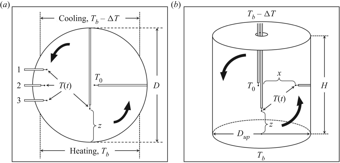
The experimental apparatus and procedures used in this work have been described in detail in previous publications (He & Tong Reference He and Tong2009; He, Ching & Tong Reference He, Ching and Tong2011; Song, Villermaux & Tong Reference Song, Villermaux and Tong2011; Wang et al. Reference Wang, He and Tong2016, Reference Wang, Lai, Song and Tong2018a,Reference Wang, Xu, He, Yik, Wang, Schumacher and Tongb, Reference Wang, He and Tong2019), and here we only mention some key features. The convection experiments are conducted in two convection cells with different geometries. As illustrated in figure 3(a), one convection cell is a vertical thin disk of diameter  $D = 188$ mm and thickness
 $L = 20$ mm, so that the aspect ratio of the cell is
 $A \equiv L/D \simeq 0.1$. Its circular cross-section is symmetrically aligned in parallel with gravity. The top and bottom thirds of the circular sidewall are made of nickel-plated copper, between which a stable temperature difference
 $\Delta T$ is maintained during the experiment. The rest of the cell is made of transparent Plexiglas. When the convection system reaches a steady state, an LSC of thermal plumes is established in the quasi-two-dimensional rotation plane of the convective flow, as indicated by the two black arrows in figure 3(a).
Sketch of the experimental set-up for the measurement of local temperature fluctuations at different locations in (a) the vertical thin disk and (b) the  $A=1$ upright cylinder. In the thin disk cell, the local temperature time series data
 $T(t)$ are measured by waterproof thermistors along the vertical axis of the cell with varying distance
 $z$ from the bottom plate and at three fixed vertical positions close to the sidewall. The measurements of
 $T(t)$ in the upright cylinder are conducted along the vertical axis of the cell with varying distance
 $z$ and along the radial direction with varying distance
 $x$ at the mid-plane of the cylinder. The black arrows indicate the direction of the large-scale circulation. The coordinate system used is also shown.

As illustrated in figure 3(b), the other convection cell is an upright cylinder whose sidewall is made of transparent Plexiglas with inner diameter  $D_{{up}} = 190$ mm and height
 $H = 190$ mm, so that the aspect ratio of the cylinder is
 $A \equiv D_{{up}}/H = 1$. The cylindrical sidewall is sandwiched between two gold-plated brass plates, and a stable temperature difference
 $\Delta T$ is maintained between them. During the experiment, the convection cells are placed inside a square thermostat box, in which the temperature is maintained the same as the mean temperature
 $T_{{bulk}}$ of the bulk convecting fluid. This set-up minimizes the heat exchange and thermal interference between the bulk fluid and surroundings.
Because of the different shapes and aspect ratios, the two convection systems have different flow structures. First, the LSC in the upright cylinder has more complex three-dimensional modes, such as torsional and sloshing modes (Funfschilling & Ahlers Reference Funfschilling and Ahlers2004; Xi et al. Reference Xi, Zhou, Zhou, Chan and Xia2009), which are absent in the quasi-two-dimensional thin disk (Wang et al. Reference Wang, He and Tong2016). As the thermal plumes are carried by the LSC, the spatial distributions of thermal plumes in the two cells are different. Second, the boundary layer dynamics in the two cells is different (one has corner flows and the other has no corner flow) (Wang et al. Reference Wang, Xu, He, Yik, Wang, Schumacher and Tong2018b), which affects the emission dynamics of thermal plumes. These two features are important in determining the spatial variations of temperature fluctuations and their p.d.f.s. We therefore use the two convection cells to test the theory more thoroughly.
For the thin disk cell, its  ${\textit {Ra}}$ is defined with the cell height
 $H$ being replaced by the disk diameter
 $D$. By varying
 $\Delta T$, we change the values of
 ${\textit {Ra}}$ in the range
 $8 \times 10^{8} \lesssim {\textit {Ra}} \lesssim 1.3 \times 10^{10}$. Two working fluids are used in the experiment. For the measurements in the thin disk, we use distilled water and a 20 wt.
 $\%$ aqueous solution of glycerin at
 $T_{{bulk}} = 40\,^{\circ }$C. The corresponding Prandtl numbers are
 ${\textit {Pr}} = 4.4$ for water and
 ${\textit {Pr}} = 7.6$ for glycerin solution. For the measurements in the upright cylinder, we use the glycerin solution with
 ${\textit {Pr}} =7.6$ and distilled water with
 ${\textit {Pr}}= 4.4$ (at
 $T_{{bulk}} = 40\,^{\circ }$C) and
 ${\textit {Pr}}=5.4$ (at
 $T_{{bulk}} = 30\,^{\circ }$C). Both convection cells are slightly tilted with their vertical axis at a small angle (
 ${<}1^{\circ }$) relative to gravity, which ensures that the LSC rotates anticlockwise as illustrated by the two black arrows in figures 3(a) and 3(b). On average, the LSC produces an azimuthal upward flow of warm plumes on one side of the cell and a downward flow of cold plumes on the other side of the cell. Otherwise, the small tilt has no other effect on our results (Ahlers, Brown & Nikolaenko Reference Ahlers, Brown and Nikolaenko2006).
Small glass-encapsulated thermistors of diameter 0.17 mm and accuracy 5 mK are used to measure local temperature fluctuations  $T(t)$ at different locations in the rotation plane of LSC. The procedures used for temperature calibration and measurements have been reported in detail by He & Tong (Reference He and Tong2009). As shown in figure 3, several thermistors are guided into the convection cell via stainless steel tubes. Each thermistor is mounted on a translational stage of 50
 $\mathrm {\mu }$m in spatial resolution. For the thin disk cell, one thermistor is placed at the cell centre to measure the centre temperature
 $T_0(t)$ at a sampling rate of 2 Hz. Another thermistor is used to measure
 $T(z,t)$ at varying vertical positions
 $z$ along the cell axis at a sampling rate of 15 Hz. For each value of
 $z$, we take a 1 h-long time series of
 $T(z,t)$ (
 $5.4\times 10^4$ data points). Three more thermistors are placed at different heights close to the sidewall along the flow direction of falling cold plumes. The middle thermistor is placed at the mid-plane of the cell, and the other two are placed above and below the middle one, with an equal vertical separation of 15 mm. All of the three thermistors have the same radial distance
 $r=84$ mm (
 $r/D \simeq 0.45$) away from the cell centre. Temperature measurements at the three positions are sampled at 40 Hz, and each set of time series data
 $T(t)$ is 8 h long (
 $1.2\times 10^6$ data points). For the upright cylinder, we measure
 $T(z,t)$ along the vertical axis of the cell with varying
 $z$, and
 $T(x,t)$ along the cell diameter at the mid-height with varying
 $x$, a horizontal distance away from the sidewall as shown in figure 3(b). In these temperature measurements, the sampling rate of
 $T(t)$ is 40 Hz and we typically take an 8 h-long time series for each data set (
 $\sim 10^6$ data points). From each set of time series data, we compute the local mean temperature
 $\langle T\rangle$ and its r.m.s. value
 $\sigma _T$. In the following analysis, the local temperature fluctuation
 $\delta T$ is defined as
 $\delta T(t)=T(t)-\langle T\rangle$, and the normalized local temperature fluctuation is defined as
 $\xi =\delta T/\sigma _T$.
4. Experimental results
In this section, we compare the measured  $P(\delta T)$ at various locations in the two convection cells with the theoretical model.
4.1. Turbulent temperature fluctuations in the  $A=1$ upright cylinder

We first examine the functional form of the measured  $P(\delta T)$ in the two multi-plume regions of the upright cylinder, namely, the outer BL (
 $1\lesssim z/\delta \lesssim 4$) and the side-wall region (
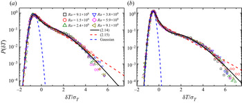
 $0.3\lesssim |x|/D\lesssim 0.5$). Figure 4 shows the p.d.f.s
 $P(\delta T)$ as functions of the normalized temperature fluctuations
 $\delta T/\sigma _T$ in the outer BL. Once the position
 $z$ is normalized by the BL thickness
 $\delta$, and
 $\delta T$ is normalized by its r.m.s. value
 $\sigma _T$, the measured p.d.f.s
 $P(\delta T)$ for different values of
 ${\textit {Ra}}$ at a given normalized position
 $z/\delta$ all collapse onto a single master curve, indicating that
 $\sigma _T$ and
 $\delta$ are the proper scaling variables for
 $P(\delta T)$ (Wang et al. Reference Wang, He and Tong2016, Reference Wang, Xu, He, Yik, Wang, Schumacher and Tong2018b). The left-hand side of the peak in
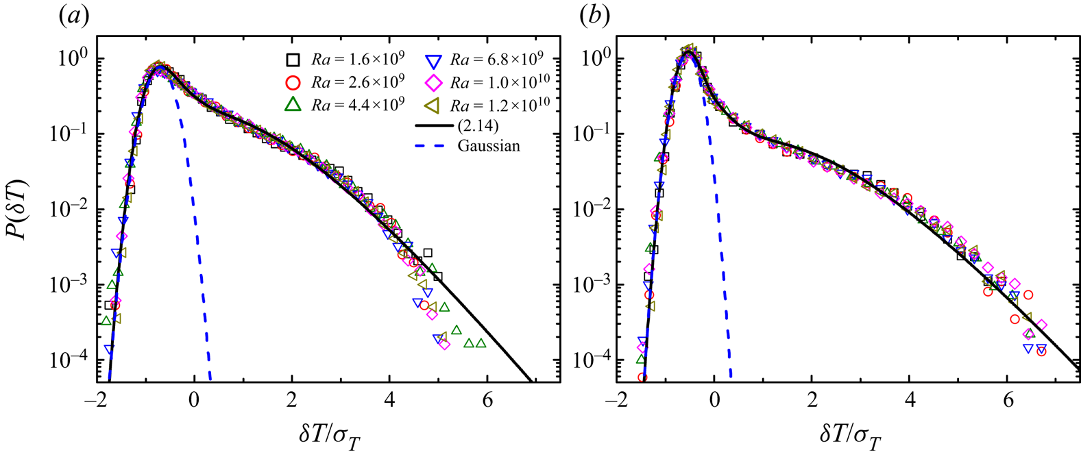
 $P(\delta T)$ has a Gaussian shape (blue dashed lines), which we believe results from the residual temperature fluctuations caused by thermal conduction inside the BL (close to the bottom conducting plate). When the warm plumes form and are emitted into the outer BL, they start to dominate the temperature fluctuations on the right-hand side of the peak in
 $P(\delta T)$, which is highly non-Gaussian. As shown by the black solid lines in figure 4, (2.14) fits the data well with four fitting parameters at both locations. For comparison, we also plot in figure 4 the fits of (2.15) to the data points (red dashed lines), which include only the contributions of single plumes; multi-plume contributions are excluded. It is seen that (2.15) gives rise to a straight exponential tail for large
 $\delta T$ (
 $\delta T/\sigma _T\gtrsim 0$) and cannot well describe the downward-bending tail of the measured
 $P(\delta T)$ (for
 $\delta T/\sigma _T\gtrsim 1$). The fitting results shown in figure 4 thus demonstrate the existence of the multi-plume effect and its significance in determining the functional form of
 $P(\delta T)$.
Measured p.d.f.s  $P(\delta T)$ as functions of the normalized temperature fluctuations
 $\delta T/\sigma _T$ for different values of
 ${\textit {Ra}}$ at a fixed
 ${\textit {Pr}}=7.6$ (20 wt.% aqueous solution of glycerin). The measurements were made in the outer BL region along the central vertical axis of the
 $A=1$ upright cylinder at a fixed normalized distance, (a)
 $z/\delta \simeq 1.3$ and (b)
 $z/\delta \simeq 2.2$, away from the bottom conducting plate. The black solid lines show the fits of (2.14) to the data points in (a) with
 $\alpha _w=0.45\pm 0.05$,
 $n_w=4.8\pm 0.5$,
 $\beta _{sw}=0.75\pm 0.05$,
 $\beta _{mw}=0.25\pm 0.05$, and in (b) with
 $\alpha _w=0.40\pm 0.05$,
 $n_w=6.0\pm 0.5$,
 $\beta _{sw}=0.50\pm 0.1$,
 $\beta _{mw}=0.13\pm 0.02$. The red dashed lines show plots of (2.15) in (a) with
 $\alpha _w=0.20$,
 $\beta _{sw}=0.80$, and in (b) with
 $\alpha _w=0.16$,
 $\beta _{sw}=0.45$. The blue dashed lines in (a,b) show a Gaussian distribution.

It is found that the fitted value of  $\alpha _w$ decreases with increasing
 $z/\delta$, suggesting that the effect of thermal conduction is weakened. This is expected because the thermal conduction is concentrated mainly in the inner BL and decays quickly as the measuring position moves away from the bottom conducting plate. Meanwhile, the average number of plumes
 $n_w$ in the multi-plume clusters increases with
 $z/\delta$, which indicates that in the outer BL the number of multi-plumes passing thorough the measuring position increases with
 $z/\delta$. As
 $z/\delta$ increases, the values of
 $\beta _{sw}$ and
 $\beta _{mw}$ (or
 $\beta _{sw}+\beta _{mw}$) decrease, suggesting that warm plumes become more intermittent in time. We used the least-squares fitting method with various initial values of the fitting parameters, and the best results are obtained using the manual fit based on our own fitting experience, which tends to give a global optimum. This is especially true for the most general form of (2.13) with eight fitting parameters. The error bar of the fitting parameters given in the figure captions and in table 1 below represents the confidence interval of the physical parameters that we obtain from the fitting.
Obtained representative values of the eight fitting parameters,  $\alpha _w$,
 $\alpha _c$,
 $n_w$,
 $n_c$,
 $\beta _{sw}$,
 $\beta _{mw}$,
 $\beta _{sc}$ and
 $\beta _{mc}$, in (2.13) for different flow regions in the lower half of the
 $A=1$ upright cylinder. Distilled water was used as a working fluid, and its value of
 ${\textit {Pr}}$ varies with the bulk fluid temperature. When a fluctuation mode is absent, its duty-cycle parameter
 $\beta$ is set to zero and the corresponding amplitude
 $\alpha$ and the average number of plumes
 $n$ in the multi-plume clusters are marked as N/A. The fitting results in the mixing zone, turbulent bulk and cell centre are adopted from Wang et al. (Reference Wang, He and Tong2019).

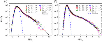
Figure 5 shows the p.d.f.s  $P(\delta T)$ as functions of
 $\delta T/\sigma _T$ at a fixed
 ${\textit {Pr}}=4.4$ (water). Similar to figure 4, the measured p.d.f.s
 $P(\delta T)$ as functions of
 $\delta T/\sigma _T$ have a
 ${\textit {Ra}}$-independent form and are well described by (2.14) (solid lines). As
 $z/\delta$ increases, the fitting parameters obtained at
 ${\textit {Pr}}=4.4$ change in a way similar to those at
 ${\textit {Pr}}=7.6$, indicating that the functional form of
 $P(\delta T)$ is not sensitive to the change in
 ${\textit {Pr}}$ in the range studied. Similar to the red dashed lines in figure 4, (2.15) – which includes only the contributions of single plumes – does not fit the p.d.f.s in figure 5 well (not shown here).
Measured p.d.f.s  $P(\delta T)$ as functions of
 $\delta T/\sigma _T$ for different values of
 ${\textit {Ra}}$ at a fixed
 ${\textit {Pr}}=4.4$ (water). The measurements were made in the outer BL region along the central vertical axis of the
 $A=1$ upright cylinder at a fixed normalized distance, (a)
 $z/\delta \simeq 1.3$ and (b)
 $z/\delta \simeq 2.5$, away from the bottom conducting plate. The black solid lines show the fits of (2.14) to the data points in (a) with
 $\alpha _w=0.45\pm 0.1$,
 $n_w=4.5\pm 1$,
 $\beta _{sw}=0.72\pm 0.05$,
 $\beta _{mw}=0.28\pm 0.05$, and in (b) with
 $\alpha _w=0.40\pm 0.05$,
 $n_w=5.0\pm 0.5$,
 $\beta _{sw}=0.40\pm 0.1$,
 $\beta _{mw}=0.15\pm 0.03$. The blue dashed lines in (a,b) show a Gaussian distribution.

We now examine the functional form of the p.d.f.s  $P(\delta T)$ obtained in the sidewall region at the mid-height (
 $z/H = 0.5$) of the
 $A=1$ upright cylinder. Figure 6 shows the p.d.f.s
 $P(\delta T)$ as functions of
 $\delta {T}/\sigma _T$ at two representative radial locations. Once the horizontal position
 $x$ is normalized by the cell diameter
 $D_{{up}}$ and
 $\delta T$ is normalized by its r.m.s. value
 $\sigma _T$, the measured p.d.f.s
 $P(\delta T)$ for different values of
 ${\textit {Ra}}$ at a given normalized position
 $x/D_{{up}}$ all fall onto a single master curve, indicating that
 $\sigma _T$ and
 $D_{{up}}$ are the proper scaling variables for
 $P(\delta T)$. A similar situation was found for the p.d.f.s
 $P(\delta T)$ measured outside the thermal BL along the vertical axis of the cell, where the cell height
 $H$ is the proper scaling length (Wang et al. Reference Wang, He and Tong2019). Because of the LSC, warm plumes accumulate on the rising side of the LSC (right-hand side of the cell as shown in figure 3b) and produce many up-rising (positive) temperature fluctuations. As a result, the most probable value of
 $\delta T$ becomes negative (smaller than the mean value of
 $T(t)$) and the p.d.f.
 $P(\delta T)$ is skewed toward the positive side. A unique feature of the measured
 $P(\delta T)$ in the sidewall region is that both single and multiple warm and cold plumes are involved in the total temperature fluctuations
 $\delta T(t)$. Consequently, all four fluctuation modes are important in (2.1), and they produce the most complex form of
 $P(\delta T)$ in the convection cell, as shown in figure 6.
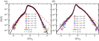
Measured p.d.f.s  $P(\delta T)$ as functions of
 $\delta T/\sigma _T$ for different values of
 ${\textit {Ra}}$ at a fixed
 ${\textit {Pr}}=5.4$ (water). The measurements were made at the mid-height (
 $z/H = 0.5$) of the
 $A=1$ upright cylinder in the sidewall region with a fixed radial distance, (a)
 $x/D_{{up}} \simeq 0.45$ and (b)
 $x/D_{{up}} \simeq 0.39$, away from the cell centre. The solid lines show the fits of (2.13) to the data points in (a) with
 $\alpha _w=1.4\pm 0.2$,
 $\alpha _c=1.3\pm 0.2$,
 $n_w=5.5\pm 1.0$,
 $n_c=5.8\pm 1.0$,
 $\beta _{sw}=0.48\pm 0.15$,
 $\beta _{mw}=0.52\pm 0.15$,
 $\beta _{sc}=0.08\pm 0.05$,
 $\beta _{mc}=0.03\pm 0.01$, and in (b) with
 $\alpha _w=0.75\pm 0.1$,
 $\alpha _c=0.65\pm 0.1$,
 $n_w=4.2\pm 1.0$,
 $n_c=3.5\pm 1.0$,
 $\beta _{sw}=0.50\pm 0.15$,
 $\beta _{mw}=0.25\pm 0.05$,
 $\beta _{sc}=0.08\pm 0.04$,
 $\beta _{mc}=0.01\pm 0.005$. The red dashed lines show the plots of (2.13) with
 ${\beta _{mw} = \beta _{mc} = 0}$ and hence
 $n_w$ and
 $n_c$ are not applicable. The red dashed line in (a) is plotted with
 $\alpha _w=0.4$,
 $\alpha _c=0.5$,
 $\beta _{sw}=1$,
 $\beta _{sc}=0.2$, and that in (b) is plotted with
 $\alpha _w=0.3$,
 $\alpha _c=0.4$,
 $\beta _{sw}=1$,
 $\beta _{sc}=0.1$.

The solid lines in figure 6 show the fits of (2.13) to the measured p.d.f.s  $P(\delta T)$ with eight fitting parameters. An excellent agreement between the theoretical model and experimental results is obtained. At each radial distance
 $x/D_{{up}}$, the fitted values of
 $\alpha _w$ and
 $n_w$ for warm plumes are close to those (
 $\alpha _c$ and
 $n_c$) for cold plumes, indicating that the strength and superposition level of multiple warm and cold plume clusters are approximately the same. Meanwhile, the duty-cycle parameters
 $\beta _{sw}$ and
 $\beta _{mw}$ for warm plumes are much larger than those (
 $\beta _{sc}$ and
 $\beta _{mc}$) for cold plumes, which suggests that there are more warm plumes passing through the measuring position than the cold plumes. This is expected as the temperature measurements are conducted on the rising side of the LSC, as shown in figure 3(b), where there are more warm plumes rising with the LSC than the cold plumes falling downwards against the LSC. When the radial location is moved closer to the cell centre (smaller value of
 $x/D_{{up}}$), the fitted values of
 $\alpha _w$,
 $\alpha _c$,
 $n_w$,
 $n_c$,
 $\beta _{mw}$ and
 $\beta _{mc}$ become smaller. These results suggest that the incidence of multi-plume clusters and the average number of plumes in them are reduced, whereas the fluctuation strength of thermal plumes relative to the background increases. The values of
 $\beta _{sw}$ and
 $\beta _{sc}$ do not show a strong dependence on the two values of
 $x/D_{{up}}$ studied. For comparison, we also plot in figure 6 the fits of (2.13) without the multi-plume modes (
 $\beta _{mw}=\beta _{mc}=0$) to the data points (red dashed lines), which cannot well describe the downward-bending tails of the measured p.d.f.s. The fitting results shown in figure 6 thus demonstrate the existence of the multi-plume effect in the sidewall region and its significance in determining the functional form of
 $P(\delta T)$.
4.2. Turbulent temperature fluctuations in the thin disk cell
Figure 7 shows the p.d.f.s  $P(\delta T)$ as functions of
 $\delta T/\sigma _T$ in the outer BL. Similar to the situation for the upright cylinder, the measured p.d.f.s
 $P(\delta T)$ for different values of
 ${\textit {Ra}}$ at a given normalized position
 $z/\delta$ all collapse onto a single master curve, once
 $\delta T$ is normalized by its r.m.s. value
 $\sigma _T$. The left-hand side of the peak in
 $P(\delta T)$ has a Gaussian shape (blue dashed lines), but the right-hand side of the peak in
 $P(\delta T)$ is highly non-Gaussian. It decays much slower than a Gaussian function but faster than a simple exponential function. As mentioned above, this is a signature of temperature fluctuations
 $\delta T_{mw}$ resulting from the multiple warm plumes, which follow the gamma distribution. It is seen that the obtained p.d.f.s at both locations in the outer BL can be well described by (2.14) with four fitting parameters (solid lines). Similar to the red dashed lines in figure 4, (2.15) – which includes only the contributions of single plumes – does not fit the data in figure 7 well (not shown here).
Measured p.d.f.s  $P(\delta T)$ as functions of
 $\delta T/\sigma _T$ for different values of
 ${\textit {Ra}}$ at a fixed
 ${\textit {Pr}}=7.6$ (20 wt.% aqueous solution of glycerin). The measurements were made in the outer BL region along the central vertical axis of the thin disk cell at a fixed normalized distance, (a)
 $z/\delta \simeq 1.3$ and (b)
 $z/\delta \simeq 2.2$, away from the bottom conducting plate. The black solid lines show the fits of (2.14) to the data points in (a) with
 $\alpha _w=0.67\pm 0.07$,
 $n_w=5.5\pm 0.8$,
 $\beta _{sw}=0.75\pm 0.15$,
 $\beta _{mw}=0.065\pm 0.02$, and in (b) with
 $\alpha _w=0.45\pm 0.05$,
 $n_w=6.0\pm 1$,
 $\beta _{sw}=0.35\pm 0.15$,
 $\beta _{mw}=0.046\pm 0.01$. The blue dashed lines in (a,b) show a Gaussian distribution.

As  $z/\delta$ increases, the fitted values of
 $\beta _{sw}$,
 $\beta _{mw}$,
 $\alpha _w$ and
 $n_w$ in the thin disk show a trend similar to those for the
 $A=1$ upright cylinder. With increasing
 $z/\delta$, the relative strength of warm plumes, as expressed by
 $\alpha _w^{-1}$, increases in agreement with the fact that the right-hand side of the peak in
 $P(\delta T)$, as shown in figure 7(b), is skewed further to the right. The two duty-cycle parameters
 $\beta _{sw}$ and
 $\beta _{mw}$ decrease with increasing
 $z/\delta$, indicating that the warm plumes become more intermittent as they move away from the BL. At the same location
 $z/\delta$ and same
 ${\textit {Pr}}$, the obtained value of
 $\beta _{mw}$ in the thin disk is much smaller than that in the upright cylinder, suggesting that the warm plume clusters appear less frequently in the thin disk. There are two possible reasons for this effect. First, the LSC in the upright cylinder has a three-dimensional motion (Funfschilling & Ahlers Reference Funfschilling and Ahlers2004; Xi et al. Reference Xi, Zhou, Zhou, Chan and Xia2009), which may bring extra plumes from the nearby region to the measuring position, thereby increasing the incidence of the multiple plumes. Second, the outer BL region in the thin disk (
 $1 \lesssim z/\delta \lesssim 2$) is narrower than that in the upright cylinder (
 $1 \lesssim z/\delta \lesssim 4$) (Wang et al. Reference Wang, He and Tong2016, Reference Wang, Xu, He, Yik, Wang, Schumacher and Tong2018b). As a result, the measuring position in the thin disk is relatively closer to the mixing zone compared with that in the upright cylinder with the same value of
 $z/\delta$, which leads to a reduced probability of detecting the multi-plume clusters in the thin disk.
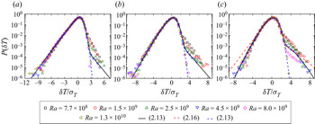
Finally, we examine the functional form of the p.d.f.s  $P(\delta T)$ obtained in the sidewall region. Figures 8(a), 8(b) and 8(c) show, respectively, the p.d.f.s
 $P(\delta T)$ obtained at three fixed positions along the flow direction of LSC, where there are more cold plumes falling along the LSC than warm plumes rising against the LSC. As illustrated in figure 3(a), cold plumes accumulate on the left-hand side of the cell (the falling side of the LSC) and produce many downward spikes in the measured
 $T(t)$. As a result, the most probable value of
 $\delta T$ becomes slightly positive (larger than the mean value of
 $T(t)$), and the p.d.f.
 $P(\delta T)$ is skewed towards the negative side. The main portion of the measured p.d.f.s
 $P(\delta T)$ (with
 $\delta T/\sigma _T \lesssim 2$) for different values of
 ${\textit {Ra}}$ falls onto a single master curve, once
 $\delta T$ is normalized by its r.m.s. value
 $\sigma _T$. This result suggests that the statistics of cold plumes and turbulent background are invariant in the
 ${\textit {Ra}}$ range studied. On the other hand, the positive (right) tail of the measured p.d.f.s
 $P(\delta T)$ (with
 $\delta T/\sigma _T \gtrsim 2$) varies with
 ${\textit {Ra}}$, suggesting that the statistics of warm plumes are influenced by the changes in
 ${\textit {Ra}}$. This is because the LSC in the thin disk is more organized compared with that in the upright cylinder, so that fewer warm plumes will move against the LSC and reach the measuring positions with increasing
 ${\textit {Ra}}$. It is seen that when
 ${\textit {Ra}} \simeq 1.3\times 10^{10}$, the measured p.d.f.s
 $P(\delta T)$ at the three positions all reach their asymptotic form.
Measured p.d.f.s  $P(\delta T)$ as functions of
 $\delta T/\sigma _T$ for different values of
 ${\textit {Ra}}$ at a fixed
 ${\textit {Pr}}=4.4$ (water). The temperature measurements were conducted at three fixed positions in the sidewall region of the thin disk cell, as indicated in figure 3(a): (a) position 1, (b) position 2, and (c) position 3. All the three positions have the same radial distance
 $r=84$ mm (
 $r/D \simeq 0.45$) away from the cell centre. The black solid lines show the fits of (2.13) to the data points obtained at
 ${\textit {Ra}}=4.5\times 10^{9}$ (blue down-pointing triangles) in (a) with
 $\alpha _w=0.57\pm 0.05$,
 $\alpha _c=0.65\pm 0.1$,
 $n_c=1.3\pm 0.3$,
 $\beta _{sw}=0.0025\pm 0.001$,
 $\beta _{mw}=\beta _{sc}=0$,
 $\beta _{mc}=1$, in (b) with
 $\alpha _w=0.6\pm 0.08$,
 $\alpha _c=1.0\pm 0.15$,
 $n_c=2.5\pm 1.0$,
 $\beta _{sw}=0.008\pm 0.002$,
 $\beta _{mw}=\beta _{sc}=0$,
 $\beta _{mc}=1$, and in (c) with
 $\alpha _w=1.1\pm 0.1$,
 $\alpha _c=1.2\pm 0.1$,
 $n_w=6.0\pm 0.7$,
 $n_c=4.5\pm 1.0$,
 $\beta _{sw}=0.02\pm 0.01$,
 $\beta _{mw}=0.003\pm 0.001$,
 $\beta _{sc}=0$,
 $\beta _{mc}=1$. For solid lines in (a,b),
 $n_w$ is not applicable as
 $\beta _{mw}=0$. The blue dashed lines show the fits of (2.13) to the data points obtained at
 ${\textit {Ra}}=1.3\times 10^{10}$ (brown left triangles) in (a) with
 $\alpha _c=0.65\pm 0.1$,
 $n_c=1.3\pm 0.3$, in (b) with
 $\alpha _c=1.0\pm 0.2$,
 $n_c=2.5\pm 1.0$, and in (c) with
 $\alpha _c=1.2\pm 0.2$,
 $n_c=4.5\pm 1.5$. For all the blue dashed lines, we find
 $\beta _{sw}=\beta _{mw}=\beta _{sc}=0$ and
 $\beta _{mc}=1$. Consequently,
 $\alpha _w$ and
 $n_w$ are not applicable. The red dashed line in (c) shows the plot of (2.16) with
 $\alpha _w=0.5$,
 $\alpha _c=0.85$ and
 $\beta _{sw}=0.012$.

The solid lines in figure 8 show the fits of (2.13) to the p.d.f.s  $P(\delta T)$ obtained at the three positions with a given value of
 ${\textit {Ra}} = 4.5\times 10^9$. An excellent agreement between the theoretical model and experimental data is obtained with the given fitting parameters. Equally good fits are also obtained to the p.d.f.s
 $P(\delta T)$ obtained at other values of
 ${\textit {Ra}}$ (not shown here). Unlike the sidewall region in the upright cylinder, which contains both intermittent single and multiple plumes, we find
 $\beta _{sc}=0$ and
 $\beta _{mc}=1$ from the fits at all three positions in the sidewall region of the thin disk. This result suggests that single cold plumes are absent on the down side of the LSC, and multiple cold plumes are continuous in time, further confirming that the LSC in the thin disk is more organized compared with that in the upright cylinder. As the measuring position moves from the up steam (position 1) to the down stream (position 3) as shown in figure 3(a), the fitted values of
 $\alpha _c$ and
 $n_c$ for the multiple cold plumes increase, indicating a decrease of cold plume strength and an increase of their average number in the multiple plume clusters. This is because the cold plumes will diffuse and mix with the surrounding fluid as they travel down stream with the LSC, a process that reduces their relative temperature difference with the background (reduction of strength) and increases their size, making them easier to cluster. The duty-cycle parameters
 $\beta _{sw}$ and
 $\beta _{mw}$ for warm plumes also increase along the down stream direction. This is expected because in the sidewall region where the warm plumes rise against the LSC, it is easier to detect them at a measuring position closer to the heating plate. Meanwhile, the fitted value of
 $\alpha _w$ increases as the measuring position moves toward the heating plate, indicating a decrease of warm plume strength. This counter-intuitive effect is also caused by the LSC, which acts as a discriminator of warm plumes. At position 1, only strong warm plumes with larger temperature variations relative to the background can reach, which gives rise to a larger plume strength. At position 3, however, weaker warm plumes with moderate temperature variations can also reach, which reduces the mean strength of warm plumes. For comparison, we also plot in figure 8(c) the fit of (2.16) to the data points at
 ${\textit {Ra}} = 4.5\times 10^9$ (blue down-pointing triangles), which includes only the contributions of single plumes; multi-plume contributions are excluded. It is clearly seen that (2.16) cannot well describe the two downward-bending tails of the measured p.d.f., further demonstrating the multi-plume effect in the sidewall region and its significance in determining the functional form of
 $P(\delta T)$.
The blue dashed lines in figure 8 show the fits of (2.13) to the p.d.f.s  $P(\delta T)$ obtained at the three positions with the largest value of
 ${\textit {Ra}} = 1.3\times 10^{10}$ achievable in the experiment. At this
 ${\textit {Ra}}$, warm plumes have been completely eliminated from the down side of LSC, and consequently, we find
 $\beta _{sw}=\beta _{mw}=\beta _{sc}=0$ and
 $\beta _{mc}=1$. In this case,
 $\alpha _w$ and
 $n_w$ are not applicable, and the p.d.f.s
 $P(\delta T/\sigma _T)$ become a convolution between the gamma distribution and a Gaussian background with only two fitting parameters. The fitted values of
 $\alpha _c$ and
 $n_c$ for the multiple cold plumes show an increasing trend similar to those for other values of
 ${\textit {Ra}}$, when the measuring position is moved from the up steam (position 1) to the down stream (position 3). At a fixed position, the measured p.d.f.s
 $P(\delta T)$ have reached their asymptotic form, and thus the fitted values of
 $\alpha _c$ and
 $n_c$ become invariant with
 ${\textit {Ra}}$.
5. Summary
In this paper, we report a systematic study of the collective effect of thermal plumes on the p.d.f.  $P(\delta T)$ of turbulent temperature fluctuations
 $\delta T(t)$ in a closed Rayleigh–Bénard convection cell. To include the effect of multiple plumes appearing simultaneously at the measuring position, we assume that the plume-induced temperature fluctuations
 $\delta T_P(t)$ can be decomposed into four independent fluctuation modes, as shown in (2.1). Temperature fluctuations produced by single warm (or cold) plumes follow the exponential distribution, whereas those produced by multiple warm (or cold) plumes obey the gamma distribution. In addition, the overall temperature fluctuations,
 $\delta T(t)=\delta T_P(t)+\delta T_B(t)$, contain a turbulent background
 $\delta T_B(t)$, which follows the Gaussian distribution. With this decomposition, we derive the general form of
 $P(\delta T)$ in (2.13) from the convolutions of the five independent fluctuation modes. The derived form of
 $P(\delta T)$ includes eight space-dependent parameters, which account for the spatial variations of the number of plumes in multiple plume clusters and their relative strengths and degrees of intermittency. Equation (2.1) can be simplified to (2.14)–(2.18) when one or more fluctuation modes become negligibly small. In particular, when the multiple-plume effect can be neglected, (2.1) becomes (2.16), which has been verified in a previous experiment conducted in the single-plume regions of the convection flow (Wang et al. Reference Wang, He and Tong2019).
To test the derived form of  $P(\delta T)$ in the multiple-plume regions, we conducted new temperature measurements in two convection cells; one is the vertical thin disk and the other is the
 $A=1$ upright cylinder. The convection experiments were conducted in the
 ${\textit {Ra}}$ range
 $8 \times 10^8 \lesssim {\textit {Ra}} \lesssim 1.3\times 10^{10}$, and at three fixed values of
 ${\textit {Pr}} = 4.4$,
 $5.4$ and
 $7.6$. The two multiple-plume regions studied are the sidewall region at the mid-height of the cell and the outer BL region with
 $1 \lesssim z/\delta \lesssim 2$ for the thin disk and
 $1 \lesssim z/\delta \lesssim 4$ for the upright cylinder, in which the thermal plumes are heavily populated. For a given normalized position, all of the measured p.d.f.s
 $P(\delta T)$ fall onto a single master curve, once
 $\delta T$ is normalized by its r.m.s. value
 $\sigma _T$. In the outer BL region near the bottom conducting plate, negative fluctuations (
 $\delta T \lesssim 0$) are from the turbulent background, which follows the Gaussian distribution. Positive fluctuations (
 $\delta T \gtrsim 0$), on the other hand, are produced by both single and multiple warm plumes, which give rise to a highly non-Gaussian
 $P(\delta T)$. The measured temperature p.d.f.s
 $P(\delta T)$ are well described by (2.14), which includes the contributions from the turbulent background, and single and multiple warm plumes.
In the sidewall region, both the single and multiple warm and cold plumes contribute to the measured  $P(\delta T)$. Large temperature fluctuations are evident on both the positive and negative tail parts of the measured
 $P(\delta T)$. They are neither Gaussian nor exponential and give rise to the most complex form of temperature p.d.f. in the convection cell, as shown in figures 6 and 8. The measured temperature p.d.f.s
 $P(\delta T)$ are well described by (2.13), which includes all of the five fluctuation modes given in (1.4) and (2.1); each has its own distinct distribution, as shown in (2.2)–(2.7). The eight fitting parameters in (2.13) are closely related to the spatial distribution of thermal plumes and local dynamics of the LSC in a closed convection cell and therefore they have clear physical interpretations.
Table 1 gives a brief summary of the representative values of the eight fitting parameters in (2.13), which are obtained from the five flow regions in the lower half of the  $A=1$ upright cylinder. Inside each flow region, the fitted values of the parameters still change continuously to a certain extent. For different flow regions, the fitted values of the four duty-cycle parameters show categorical changes, representing different states regarding the four plume-related modes, with 0 indicating non-existence, 1 indicating continuous existence, and a value between 0 and 1 indicating intermittent existence. The data in the last row of table 1 were obtained at a slightly different Prandtl number (
 ${\textit {Pr}}=5.4$). It has been shown that such a small change in
 ${\textit {Pr}}$ will not cause a large change in the fitting parameters (Wang et al. Reference Wang, He and Tong2019). The fitting results shown in table 1 provide an overall description of the measured
 $P(\delta T)$ in different flow regions. It is found that the fitted values of
 $\alpha _w$ and
 $\alpha _c$ in the sidewall region are much larger than those along the central axis, indicating that the sidewall region has a relatively stronger turbulent background. The fitted values of
 $n_w$ in the outer BL (
 $n_w=5.0$) are close to those in the sidewall (
 $n_w=5.5$). This result indicates that most warm plumes emitted from the bottom BL are carried to the sidewall region, as expected.
Our work thus further demonstrates that temperature fluctuations in turbulent RBC can indeed be decomposed into four basic fluctuation modes plus a turbulent background based on the statistics of thermal plumes. The final functional form of the temperature p.d.f.  $P(\delta T)$, which results from the convolutions of the five independent modes, is closely linked to the spatial distribution of thermal plumes and local dynamics of the LSC in a closed convection cell. This systematic approach to understanding scalar p.d.f.s in a turbulent field is very useful not only for the present study but also for the study of many turbulent mixing problems of practical interest. For example, it is worth testing the effectiveness of our model in turbulent RBC with
 ${\textit {Pr}}<1$ (Wei Reference Wei2021), where the viscous BL is nested inside the thermal BL and the plume distribution changes considerably (Xu et al. Reference Xu, Wang, He, Wang, Schumacher, Huang and Tong2021). By applying the model to the p.d.f.
 $P(\delta T)$ measured at two spatially symmetric positions, such as those symmetric points on the central or horizontal axis relative to the cell centre, one can check the symmetry characteristics of warm and cold plumes and their clusters. With more p.d.f. measurements, one may also investigate the two-dimensional landscape showing the variations of the eight fitting parameters in the rotation plane of the LSC. It is also interesting to examine how the new model can be used to describe temperature p.d.f.s resulting from turbulent RBC under different boundary conditions, such as surface roughness or wall slippage. Our model may also be extended to describe scalar distributions in other flow systems. Examples include dye concentration in turbulent mixing (Villermaux & Duplat Reference Villermaux and Duplat2003), and temperature fluctuations in a closed combustion chamber or those caused by plume-like drafts in the Earth's atmospheric surface layer (Chu et al. Reference Chu, Parlange, Katul and Albertson1996; Liu, Hu & Cheng Reference Liu, Hu and Cheng2011; Chowdhuri, Iacobello & Banerjee Reference Chowdhuri, Iacobello and Banerjee2021).
Funding
This work was supported in part by the Hong Kong Research Grants Council under grant nos 16301719 (P.T.) and N_HKUST604/19 (P.T.). X.H. acknowledges the support of the Max Planck Partner Group, the National Natural Science Foundation of China (grant nos 11772111 and 91952101), the Natural Science Foundation of Guangdong Province (grant no. 2020A1515011094), and the Science, Technology and Innovation Commission of Shenzhen Municipality (grant no. KQJSCX20180328165817522). Y.W. acknowledges support by U.S. DoE (contract no. DE-AC02-09CH11466), NASA (grant no. NNH15AB25I), and the Max-Planck-Princeton Center for Plasma Physics (MPPC).
Declaration of interests
The authors report no conflict of interest.