

1 Introduction
Developmental dyslexia, an unexpected difficulty in accuracy or fluency of reading for an individual’s chronological age or intelligence, is the most common neurobehavioral disorder in children, affecting 17% to 21% of school-age children (Fletcher et al., Reference Fletcher, Shaywitz, Shankweiler, Katz, Liberman, Stuebing and Shaywitz1994; Ferrer et al., Reference Ferrer, Shaywitz, Holahan, Marchone and Shaywitz2010, Reference Ferrer, Shaywitz, Holahan, Marchone, Michaels and Shaywitz2015; Shaywitz et al., Reference Shaywitz, Fletcher and Shaywitz1994). At its core, dyslexia is a problem with phonological processing (getting to the elemental sounds of spoken language) that affects both spoken and written language. Dyslexia affects children and adults in both developed and developing countries (Kirsch et al., Reference Kirsch, Jungeblut, Jenkins and Kolstad1993; Elbro et al., Reference Elbro, Moller and Nielsen1995; OECD and Statistics Canada, 1995). While the effects of dyslexia are evident in school, surprisingly little is known about how dyslexia affects the everyday lives of dyslexic adults who are no longer in school.
Low levels of adult literacy have strong effects on virtually every facet of adult life. The National Adult Literacy Survey (NALS), a 1992 cross-sectional study of a nationally representative sample of U.S. adults aged 16 years and older (Sum, Reference Sum1999; Sum et al., Reference Sum, Kirsch and Yamamoto2004), found that men and women with higher levels of literacy were significantly more likely to be employed and to avoid unemployment, to be active labor-force participants, to be employed in professional, management-related and technical (rather than service, craft, and laborer/helper) occupations, to have supervisory responsibilities at their jobs; to earn significantly (two to three times) more weekly and annually; and to participate in educational and training activities. Conversely, men and women with lower levels of literacy were more likely to be poor or near poor, to rely on public assistance for financial support, and to experience chronic health problems. In a related study, Rudd et al. (Reference Rudd, Kirsch and Yamamoto2004) linked higher health literacy scores to wealth, health, reading engagement, and civic engagement. Nevertheless, identifying the consequences of dyslexia in adults in the workplace remains an elusive problem.
Dyslexia has profound long-term impacts on educational, income, and health outcomes, all of which are significantly worse for dyslexics than for their nondyslexic peers. High-school drop-out rates for students classified as learning disabled (80% to 90% of whom are dyslexic) are three to four times as large as for typical readers (Blackorby & Wagner, Reference Blackorby and Wagner1996). Men and women with lower levels of literacy are more likely to be below or near national poverty levels (Kirsch et al., Reference Kirsch, Jungeblut, Jenkins and Kolstad1993; Reder & Vogel, Reference Reder, Vogel, Gerber and Brown1997; Rudd et al., Reference Rudd, Kirsch and Yamamoto2004, Reference Rudd, Anderson, Oppenheimer, Nath, Comings, Garner and Smith2007; Sum et al., Reference Sum, Kirsch and Yamamoto2004; Kutner et al., Reference Kutner, Greenberg, Jin, Boyle, Hsu and Dunleavy2007; Tamassia et al., Reference Tamassia, Lennon, Yamamoto and Kirsch2007; Bynner & Parsons, Reference Bynner, Parsons, Reder and Bynner2009; Kruidenier et al., Reference Kruidenier, MacArthur and Wrigley2010). In addition, adults with low levels of literacy have difficulty accessing or understanding health-related information, are hospitalized more often, and do not manage chronic diseases as well (Rudd et al., Reference Rudd, Kirsch and Yamamoto2004, Reference Rudd, Anderson, Oppenheimer, Nath, Comings, Garner and Smith2007; Kutner et al., Reference Kutner, Greenberg, Jin and Paulsen2006). Overall, they are more likely to experience poor health and a shortened life span (Baker et al., Reference Baker, Parker, Williams, Clark and Nurss1997; Rudd et al., Reference Rudd, Moeykens, Colton, Comings, Smith and Garner2000; Kutner et al., Reference Kutner, Greenberg, Jin and Paulsen2006; Marcus, Reference Marcus2006).
The effects of dyslexia on adult measures of success may be limited if either of two conditions is satisfied: (1) dyslexia-related problems are overcome later in life, or (2) there are no associations between dyslexia-related problems and future outcomes in life. We explore the extent of which dyslexia may affect adult wellbeing by investigating its impact on education, income, personal health, and life-satisfaction measures. In addition, we employ a stated-preference survey to estimate adults’ willingness to pay (WTP) to enhance specific reading and speaking skills to assess how individuals with dyslexia value potential alleviation of their condition, compared with a control group.
To our knowledge, there are no available measures of the impact of dyslexia on wellbeing. WTP has been used previously in assessing how adults with a number of health conditions value improvement (e.g., Sloan et al., Reference Sloan, Viscusi, Chesson, Conover and Whetten-Goldstein1998; Brandt et al., Reference Brandt, Felipe and Hanemann2012). The WTP methodology has not previously been used to evaluate dyslexia; we provide the first estimates of the effects of dyslexia on adult wellbeing using this measure.
We present stated-preference estimates of WTP for hypothetical treatments to improve five reading, speaking, and cognitive skills: reading speed; ability to read aloud; memory; ability to pronounce names and places correctly; and ability to rapidly retrieve facts and information. Enhancement of these skills can be valuable to dyslexic and nondyslexic individuals alike. Participants are from the Connecticut Longitudinal Study, a long-running longitudinal survey of a population cohort focusing on dyslexia. Panel members were approximately 33 years old at the time of our survey and have been continuously enrolled in the study since about age five.
We observe strong socioeconomic differences between respondents with and without dyslexia. Dyslexic individuals are less likely to have an undergraduate or graduate diploma. This difference in educational attainment may be an important contributor to the large income differences that we identify. Dyslexic individuals earn an estimated 15% less per year (around $8000) than nondyslexic individuals and have about 30% smaller net worth by age 33 than their nondyslexic counterparts (around $60,000). In addition, dyslexic individuals have worse self-reported health than nondyslexic individuals. Nevertheless, we do not observe any statistically significant difference in self-reported life satisfaction between dyslexic and nondyslexic individuals, which is consistent with hedonic adaptation as found in the life-satisfaction literature (Shane & Loewenstein, Reference Shane, Loewenstein, Kahneman, Diener and Schwarz1999).
We find that both dyslexic and nondyslexic individuals have positive WTP for all five of the skills we consider. The estimated rates of WTP per unit improvement in skill are similar, except dyslexic individuals are willing to pay significantly more than nondyslexics to improve their skill in reading aloud. Because dyslexics have on average lower skill levels than nondyslexics, their WTP to improve each skill to a common level is larger. However, dyslexic individuals’ WTP is small compared with the difference in earnings between dyslexic and nondyslexic adults. Dyslexic individuals’ average WTP for an improvement in all skills is approximately $3000, less than the estimated $8000 difference in annual earnings. Because the observed earnings differential reflects differences in educational attainment and other factors, interventions to improve skills at age 33 will not shift dyslexic individuals to the earnings trajectories they would have followed had their skills been improved as children. Nevertheless, we suspect that stated-preference estimates of the value of cognitive skills may substantially underestimate the value derived from effects on lifetime earnings and health.
The paper is organized as follows. Section 2 describes the theoretical model. Section 3 presents the empirical implementation and data. Section 4 reports results and Section 5 presents tests of validity and robustness. Section 6 concludes the paper.
2 Theoretical model
We explore individuals’ tradeoffs between wealth (which can be used for many purposes) and improvements in reading or speaking skills. Take a simple preference specification where individuals derive utility from wealth (
 $w$
) and current skill level (
 $s$
). We define the utility function as
 $u=u(w,s)$
. Using stated-preference methods, one can elicit WTP for a discrete improvement in skill. Let WTP to increase skill level by the amount
 $e$
be denoted by the compensating variation
 $C(e,w,s)$
.
Increasing skill by the amount
 $e$
while paying the amount
 $C$
leaves the individual with the same utility as forgoing the improvement:
 $$\begin{eqnarray}\displaystyle u(w-C(e,w,s),s+e)=u(w,s). & & \displaystyle\end{eqnarray}$$
We assume utility is increasing and concave in wealth (
 $\frac{\unicode[STIX]{x2202}u}{\unicode[STIX]{x2202}w}>0,\frac{\unicode[STIX]{x2202}^{2}u}{\unicode[STIX]{x2202}^{2}w}<0$
) and increasing in skill (
 $\frac{\unicode[STIX]{x2202}u}{\unicode[STIX]{x2202}s}>0$
) but make no assumptions about higher-order derivatives or cross-derivatives with respect to skill. To simplify notation, let
 $C=C(e,w,s)$
,
 $u=u(w,s)$
, and
 $U=u(w-C,s+e)$
. Differentiating (1) with respect to
 $e$
yields:
 $$\begin{eqnarray}\displaystyle \frac{\unicode[STIX]{x2202}C}{\unicode[STIX]{x2202}e}=\frac{\displaystyle \frac{\unicode[STIX]{x2202}U}{\unicode[STIX]{x2202}s}}{\displaystyle \frac{\unicode[STIX]{x2202}U}{\unicode[STIX]{x2202}w}}>0, & & \displaystyle\end{eqnarray}$$
i.e., WTP is increasing in the magnitude of the skill improvement, which is intuitive. Differentiating (1) with respect to
 $s$
yields:
 $$\begin{eqnarray}\displaystyle \frac{\unicode[STIX]{x2202}C}{\unicode[STIX]{x2202}s}=\frac{\displaystyle \frac{\unicode[STIX]{x2202}U}{\unicode[STIX]{x2202}s}-\frac{\displaystyle \unicode[STIX]{x2202}u}{\unicode[STIX]{x2202}s}}{\displaystyle \frac{\unicode[STIX]{x2202}U}{\unicode[STIX]{x2202}w}}, & & \displaystyle\end{eqnarray}$$
which implies that the effect of baseline skill on WTP for an improvement may be positive or negative. Differentiating (1) with respect to wealth yields:
 $$\begin{eqnarray}\displaystyle \frac{\unicode[STIX]{x2202}C}{\unicode[STIX]{x2202}w}=\frac{\displaystyle \frac{\unicode[STIX]{x2202}U}{\unicode[STIX]{x2202}w}-\displaystyle \frac{\unicode[STIX]{x2202}u}{\unicode[STIX]{x2202}w}}{\displaystyle \frac{\unicode[STIX]{x2202}U}{\unicode[STIX]{x2202}w}}=1-\frac{\displaystyle \frac{\unicode[STIX]{x2202}u}{\unicode[STIX]{x2202}w}}{\displaystyle \frac{\unicode[STIX]{x2202}U}{\unicode[STIX]{x2202}w}}, & & \displaystyle\end{eqnarray}$$
which also may be positive or negative. By combining expressions (2)–(4) we obtain:
 $$\begin{eqnarray}\displaystyle \left.\frac{\unicode[STIX]{x2202}C}{\unicode[STIX]{x2202}e}\right|_{e=0}\equiv \frac{\unicode[STIX]{x2202}C(0,w,s)}{\unicode[STIX]{x2202}e}=\frac{\displaystyle \frac{\unicode[STIX]{x2202}C}{\unicode[STIX]{x2202}e}-\displaystyle \frac{\unicode[STIX]{x2202}C}{\unicode[STIX]{x2202}s}}{1-\displaystyle \frac{\unicode[STIX]{x2202}C}{\unicode[STIX]{x2202}w}}>0. & & \displaystyle\end{eqnarray}$$
Equation (5) provides an exact method for computing the marginal rate of willingness to pay (MWTP) evaluated at zero improvement, using practical estimates of WTP for a nonzero improvement. The model that yields equation (5) accounts for any change in MWTP as skill improves or wealth declines as the individual buys more skill improvement.
Equation (5) reveals a link between WTP for skill improvement, skill level, and wealth. Although the signs of both the numerator and denominator are ambiguous, their ratio is always positive. This implies that the numerator and denominator have the same sign. It follows that if the increase in WTP in response to an increase in wealth is less (greater) than one for one, then the effect of baseline skill on the MWTP must be smaller (larger) than the MWTP for a skill increase. Nevertheless, without imposing more structure on the utility function, the exact relationship between WTP, wealth, and skill level is an empirical question.
3 Methods
3.1 Data
Data come from participants in the Connecticut Longitudinal Study (Shaywitz et al., Reference Shaywitz, Shaywitz, Fletcher and Escobar1990, Reference Shaywitz, Escobar, Shaywitz, Fletcher and Makuch1992, Reference Shaywitz, Fletcher, Holahan, Shneider, Marchione, Stuebing, Francis, Pugg and Shaywitz1999; Ferrer et al., Reference Ferrer, McArdle, Shaywitz, Holahan, Marchione and Shaywitz2007, Reference Ferrer, Shaywitz, Holahan, Marchone, Michaels and Shaywitz2015), a longitudinal panel of individuals focusing on dyslexia. At enrollment, individuals were representative of the children entering public kindergarten in Connecticut in 1983. For each participant, we collected information on reading from 1st to 12th grade annually and IQ scores at 3rd, 5th, 7th, 9th, and 11th grades (Woodcock & Johnson, Reference Woodcock and Johnson1977, Reference Woodcock and Johnson1989; Wechsler, Reference Wechsler1974, Reference Wechsler1981). A reading cluster score was computed using letter–word identification, word attack (decoding), and passage comprehension (Woodcock & Johnson, Reference Woodcock and Johnson1989). Dyslexia was identified as a reading cluster score 1.5 standard errors below the score predicted from the full scale IQ or a reading cluster score below 90 (Shaywitz et al., Reference Shaywitz, Escobar, Shaywitz, Fletcher and Makuch1992).
At age 33, participants were asked questions to elicit their WTP for hypothetical treatments to improve their: reading speed; ability to read aloud; memory; ability to pronounce names and places correctly; and ability to rapidly retrieve facts and information. The survey yielded
 $N=327$
completed interviews, 73% of the 445 original participants.
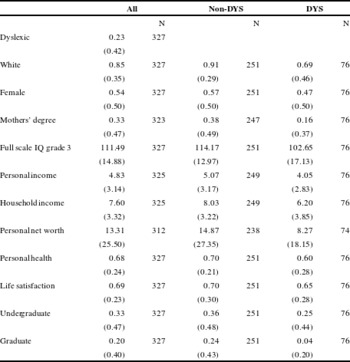
Summary statistics (Sample means and standard deviations).

Notes: DYS (dyslexic), White, Female, Undergraduate, Graduate, Mothers’ degree are indicator variables coded 1 if true and 0 otherwise. Full scale IQ is measured when the individual was in 3rd grade. Personal, household income, and net worth are in units of ten thousand dollars (2005). We summarize these responses using the midrange for each segment and the lower value for the unbounded top category. Life Satisfaction is from individuals’ agreement with the statement “I am satisfied with my life” (normalized to range from 0
 $=$
“strongly disagree” to 1
 $=$
“strongly agree”). Personal health values range from 0
 $=$
“poor” to 1
 $=$
“Excellent” health.
Table 1 provides statistics on the respondents’ demographic characteristics. Respondents are 85% white and 54% female. A third of respondents’ mothers have at least a college degree. Individuals’ full scale IQ (measured in third grade) averages 111.Footnote 1 Average annual personal income is $48,300 (2005 dollars).Footnote 2 Self-reported health, measured on a scale from 0 (poor health) to 1 (excellent), averages 0.68. Life satisfaction is elicited by asking respondents to rate how much they agree or disagree with the statement “I am satisfied with my life” using a scale from 1 (strongly disagree) to 10 (strongly agree) that we normalized to a scale from 0 to 1. The normalized score averages 0.69. Slightly over half the respondents (53%) have at least an undergraduate degree by age 33.
Following our definition, 23% of respondents have dyslexia. There are striking differences between respondents with and without dyslexia. Respondents with dyslexia are less likely to be white and female. Mothers of children with dyslexia are less educated than other mothers. Full scale IQ scores for respondents without dyslexia are on average higher than for respondents with dyslexia. There are large differences in personal income, per capita household income, and net worth between respondents with and without dyslexia. Respondents with dyslexia earn less and have lower net worth on average. Self-reported assessments on health and life satisfaction tend to be better for respondents without dyslexia than for respondents with dyslexia. Finally, respondents without dyslexia are more likely to have undergraduate and graduate degrees.
We elicited respondent’s self-reported level for each of the five skills using a scale from 1 to 5, where 5 corresponds to “very good” and 1 to “very bad.” We then elicited WTP to improve each skill individually and all five skills jointly. The skill improvement was defined as one that would raise the individual’s level on that skill to “very good.” Skill improvement was to be produced by participating in a hypothetical intervention that required engaging in two, one-hour training sessions per week, lasting for two months. The cost to the respondent was to be paid as a one-time fee and would not be covered by insurance.Footnote 3
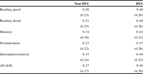
We normalized the self-reported skills to a scale from 0 to 1 and calculated the possible improvement on each skill by subtracting this transformed value from 1. We computed the “All skills” improvement as the arithmetic mean across all five skill improvements. As shown in Table 2, the hypothetical skill improvements are larger on average for dyslexics than nondyslexics and differ substantially between skills. Using the normalized scale (0 to 1), average skill improvements for dyslexic individuals range between 0.37 (for pronunciation) and 0.43 (for memory). For nondyslexics, the range is between 0.21 (for reading aloud) and 0.35 (for information retrieval). The largest difference in a self-reported skill between dyslexic and nondyslexic individuals (0.19) is for reading aloud and the smallest difference (0.05) is for information retrieval.
Self-reported skill (SRS) improvement.

Notes: Improvements for each skill are measured as the difference between self-reported skill level (SRS) and the highest SRS possible value (5) normalized to the zero-one scale. “All skills” improvement is the mean of the five individual improvements.
WTP was elicited using a double-bounded dichotomous-choice question format (Hanemann et al., Reference Hanemann, Loomis and Kanninen1991; Carson & Hanemann, Reference Carson, Hanemann, Mäler and Vincent2005; Train, Reference Train2009). Respondents were first asked if they would participate in the intervention if the cost were
 $X$
 $=$
$1000. Those who responded “yes” (they would participate) were then asked if they would participate if the cost were 2X (
 $=$
$2000); those who responded “no” to the first offer were asked if they would participate if the cost were X/2 (
 $=$
$500). To limit any effects of differences in the initial bid that could bias estimates of the relative valuation of different skills, a common value ($1000) was used as the initial bid for all skills. For logistical reasons, this same value was presented to all respondents.
3.2 Empirical strategy
We evaluate the effects of an individual’s dyslexia (denoted using the indicator variable
 $\mathit{DYS}_{i}$
) on a variety of measures of life outcomes, including personal income, household income (per capita), net worth, self-reported health, and life satisfaction. Let
 $Y$
denote an outcome variable. The effect of dyslexia on the outcome of interest can be estimated using the following OLS regression:
 $$\begin{eqnarray}\displaystyle Y_{i}=\unicode[STIX]{x1D6FC}+\unicode[STIX]{x1D702}\times \mathit{DYS}_{i}+X_{i}\times \unicode[STIX]{x1D6FE}+v_{i} & & \displaystyle\end{eqnarray}$$
where
 $X_{i}$
is a vector of demographic variables and
 $v_{i}$
rationalizes all other idiosyncratic variation. The coefficient of interest is
 $\unicode[STIX]{x1D702}$
.
We also estimate individuals’ WTP for an increase in skill. Each individual is asked to answer questions about her WTP on
 $T\;(=6)$
choice occasions. Following our theoretical model, define the observed WTP,
 $C_{it}$
(
 $e_{it}$
,
 $w_{i}$
,
 $s_{it}$
), of respondent
 $i$
on choice occasion
 $t$
for a skill improvement
 $e_{it}$
as:
 $$\begin{eqnarray}\displaystyle \text{Log}(C_{it}(e_{it},w_{i},s_{it})) & = & \displaystyle \unicode[STIX]{x1D6FD}_{1}\times e_{it}+\unicode[STIX]{x1D6FD}_{2}\times s_{it}+\unicode[STIX]{x1D6FD}_{4}\times \mathit{DYS}_{i}\nonumber\\ \displaystyle & & \displaystyle +\,\unicode[STIX]{x1D6FD}_{5}\times w_{i}+X_{i}\times \unicode[STIX]{x1D6FD}_{6}+\unicode[STIX]{x1D716}_{it},\end{eqnarray}$$
where
 $e_{it}$
,
 $s_{it}$
, and
 $w_{i}$
correspond to skill improvement, baseline skill and personal income, respectively;
 $X_{i}$
contains other individual characteristics, and
 $\unicode[STIX]{x1D716}_{it}$
rationalizes all remaining choice-to-choice individual variation.
Given the construction of our survey, skill improvement is defined as
 $e_{it}=s_{\max }-s_{it}$
, where
 $s_{\max }$
corresponds to the maximum skill level. Hence we are not able to separately identify the effects of baseline skill and skill improvement. Our estimating equation corresponds to:
 $$\begin{eqnarray}\displaystyle \text{Log}(C_{it}(e,w,s)) & = & \displaystyle \unicode[STIX]{x1D6FD}_{1}\times s_{\max }+\unicode[STIX]{x1D6FD}_{3}\times s_{it}+\unicode[STIX]{x1D6FD}_{4}\times \mathit{DYS}_{i}\nonumber\\ \displaystyle & & \displaystyle +\,\unicode[STIX]{x1D6FD}_{5}\times w_{i}+X_{i}\times \unicode[STIX]{x1D6FD}_{6}+\unicode[STIX]{x1D716}_{it},\end{eqnarray}$$
where
 $\unicode[STIX]{x1D6FD}_{1}s_{\max }$
is estimated by the intercept and
 $\unicode[STIX]{x1D6FD}_{3}$
equals the combined effects of baseline skill and skill improvement
 $(\unicode[STIX]{x1D6FD}_{2}-\unicode[STIX]{x1D6FD}_{1})$
.
Double-bounded binary-choice questions determine individuals’ WTP up to an interval (Hanemann et al., Reference Hanemann, Loomis and Kanninen1991; Carson & Hanemann, Reference Carson, Hanemann, Mäler and Vincent2005; Train, Reference Train2009). A first bid is proposed to the agent, which she can accept (“Yes”) or decline (“No”). A second question follows, in which the bid is larger if the agent accepts the initial bid and smaller otherwise. Let
 $b_{it0}$
represent the logarithm of the initial bid for individual
 $i$
at choice
 $t$
, and
 $b_{itU}$
and
 $b_{itL}$
represent the logarithms of the larger and smaller follow-up bids, respectively. Moreover, let
 $x_{i}=\{e_{i},w_{i},s_{i},X_{i}\}$
be a matrix of size
 $N\times K$
containing respondents’ characteristics. We do not observe the actual log WTP,
 $\log (C_{it}(e,w,s))$
, but rather the interval in which it is located. If we assume
 $\unicode[STIX]{x1D716}_{it}$
follows a normal distribution then the conditional probability of individual
 $i$
’s log WTP belonging to a particular interval is given by:
 $$\begin{eqnarray}\displaystyle Q_{it}(\unicode[STIX]{x1D703},x_{it},y_{it})=\left\{\begin{array}{@{}ll@{}}\unicode[STIX]{x1D6F7}\left(\displaystyle \frac{b_{itL}-x_{i}\unicode[STIX]{x1D6FD}}{\unicode[STIX]{x1D70E}}\right) & \text{if }y_{it}=0\\ \unicode[STIX]{x1D6F7}\left(\displaystyle \frac{b_{it0}-x_{i}\unicode[STIX]{x1D6FD}}{\unicode[STIX]{x1D70E}}\right)-\unicode[STIX]{x1D6F7}\left(\displaystyle \frac{b_{itL}-x_{i}\unicode[STIX]{x1D6FD}}{\unicode[STIX]{x1D70E}}\right) & \text{if }y_{it}=1\\ \unicode[STIX]{x1D6F7}\left(\displaystyle \frac{b_{itU}-x_{it}\unicode[STIX]{x1D6FD}}{\unicode[STIX]{x1D70E}}\right)-\unicode[STIX]{x1D6F7}\left(\displaystyle \frac{b_{it0}-x_{i}\unicode[STIX]{x1D6FD}}{\unicode[STIX]{x1D70E}}\right) & \text{if }y_{it}=2\\ 1-\unicode[STIX]{x1D6F7}\left(\displaystyle \frac{b_{itU}-x_{i}\unicode[STIX]{x1D6FD}}{\unicode[STIX]{x1D70E}}\right) & \text{if }y_{it}=3,\end{array}\right. & & \displaystyle \nonumber\end{eqnarray}$$
where
 $\unicode[STIX]{x1D6F7}$
is the normal cumulative distribution function,
 $\unicode[STIX]{x1D70E}$
is the standard deviation of
 $\unicode[STIX]{x1D716},\unicode[STIX]{x1D6FD}$
is a vector of coefficients, and
 $\unicode[STIX]{x1D703}=(\unicode[STIX]{x1D6FD},\unicode[STIX]{x1D70E})$
. The indicator of the choice,
 $y_{it}$
, represents responses to the two dichotomous-choice questions of “No–No,” “No–Yes,” “Yes–No,” and “Yes–Yes,” respectively. It follows that the log-likelihood function is given by:
 $$\begin{eqnarray}\displaystyle LL(\unicode[STIX]{x1D703})=\mathop{\sum }_{i=1}^{N}\mathop{\sum }_{t=1}^{T}\log (Q_{it}(\unicode[STIX]{x1D703},x_{i},y_{it})). & & \displaystyle\end{eqnarray}$$
The main identifying assumption is that respondents’ unobserved shocks are independent between respondents and choice occasions (Carson & Hanemann, Reference Carson, Hanemann, Mäler and Vincent2005). Parameters are estimated using full-information maximum likelihood.
We measure MWTP for a skill-improving intervention as dollars for a unit change in normalized skill (i.e., from “very bad”
 $=$
0 to “very good”
 $=$
1). To use equation (5) to measure MWTP requires a retransformation of our estimated coefficients. We compute the median MWTP with respect to the error term for the mean respondent. Note that the numerator of equation (5) can be computed using the following expression:
 $$\begin{eqnarray}\widehat{\frac{\unicode[STIX]{x2202}C}{\unicode[STIX]{x2202}e}-\frac{\unicode[STIX]{x2202}C}{\unicode[STIX]{x2202}s}}=-\frac{\hat{\unicode[STIX]{x1D6FD}}_{3}\exp (\bar{\unicode[STIX]{x1D707}})}{\bar{e}},\end{eqnarray}$$
where
 $\unicode[STIX]{x1D6FD}_{3}$
,
 $\bar{\unicode[STIX]{x1D707}}$
and
 $\bar{e}$
correspond to the skill coefficient from equation (8), the natural logarithm of WTP for the average respondent, and the average skill improvement, respectively. Also, note that
 $$\begin{eqnarray}\widehat{\frac{\unicode[STIX]{x2202}C}{\unicode[STIX]{x2202}w}}=\frac{\hat{\unicode[STIX]{x1D6FD}}_{5}\exp (\bar{\unicode[STIX]{x1D707}})}{\bar{e}},\end{eqnarray}$$
where
 $\unicode[STIX]{x1D6FD}_{5}$
corresponds to the income coefficient in equation (8). Median MWTP is computed as:
 $$\begin{eqnarray}\displaystyle \left.\frac{\unicode[STIX]{x2202}C}{\unicode[STIX]{x2202}e}\right|_{e=0}\equiv \frac{\unicode[STIX]{x2202}C(0,w,s)}{\unicode[STIX]{x2202}e}=-\frac{\hat{\unicode[STIX]{x1D6FD}}_{3}\exp (\bar{\unicode[STIX]{x1D707}})}{\bar{e}-\hat{\unicode[STIX]{x1D6FD}}_{5}\exp (\bar{\unicode[STIX]{x1D707}})}>0. & & \displaystyle\end{eqnarray}$$
4 Results
We begin by reporting results for the regressions describing educational attainment and other life outcomes (financial, health, and life satisfaction), followed by the regressions describing WTP for skill improvements.
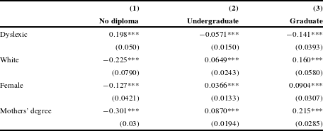
We describe educational attainment using an ordered-probit model. The dependent variable is an ordered-categorical variable with outcomes: no diploma, undergraduate diploma, and graduate diploma. Table 3 reports the estimated marginal effects of the independent variables on the outcome. The estimates suggest that dyslexia has a negative effect on educational attainment. Point estimates of the coefficients on dyslexia are negative for both undergraduate and graduate education, and positive for no diploma, and are significantly different from zero. In addition, whites and women are more likely to have completed higher education, and individuals whose mothers received an undergraduate degree are also more likely to have an undergraduate or graduate degree.
Dyslexia’s impact on education.

Notes: The number of observations is 322. The estimation is done using an ordered probit. Dependent variable is education. Regression follows from equation (6). Robust standard errors are in parentheses: * significant at 10%, ** significant at 5%, *** significant at 1%. Dyslexic, White, Female and Mothers’ degree are defined in Table 1.
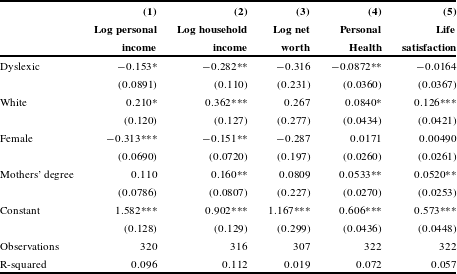
Dyslexia’s impact on income, health, and life satisfaction.

Notes: All regressions are ordinary least squares. The number of observations varies because of missing values. Regressions follow from equation (6). Robust standard errors are in parentheses: * significant at 10%, ** significant at 5%, *** significant at 1%.
Regression models for the other life-outcome variables are reported in Table 4. Independent variables are the same as in Table 3, but these models are estimated using ordinary least squares. The first three columns report results using as dependent variables the logarithm of personal income, the logarithm of per capita household income, and the logarithm of personal net worth. For these models, the estimated coefficients on dyslexia are negative but they are statistically significant only for personal and household income and not for net worth.Footnote 4 Individuals with dyslexia are estimated to have a personal income 15% smaller than individuals without dyslexia, and household per capita income and net worth are about 30% smaller. We find evidence of both racial and gender differences: the estimated coefficient of white is positive and that of female is negative in all three regressions and significant in the models for personal and household income. Compared with men, women have per capita household income 15% smaller and personal income and net worth 30% smaller (the coefficient for net worth is not significant). Point estimates of the mother’s education coefficients are positive across income measures but statistically significant only for household income.
The last two columns of Table 4 present estimates from ordinary least square regressions for self-reported health (column 4) and life satisfaction (column 5). Individuals with dyslexia report worse health than individuals without dyslexia, a statistically significant difference. The point estimate of the effect of dyslexia on life satisfaction is also negative, though not significantly so. White individuals report being healthier and feeling more satisfied with their life than nonwhite individuals. We find no statistically significant difference by gender, while mothers’ education has a positive and significant impact on both measures.
Dyslexia’s impact on self-reported potential improvements.

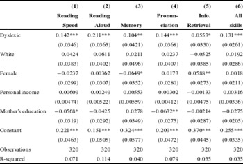
In Table 5 we report the impact of dyslexia on the level of potential improvement in each skill, defined as the difference between “very good” and the respondent’s self-reported skill level (on a 0 to 1 scale). Dyslexia has a consistently positive and statistically significant effect on all potential skill-improvement variables. Mothers’ education is negatively associated with potential improvement (i.e., positively associated with skill level) for reading speed and pronunciation. Women report smaller potential improvement in memory and larger potential improvement in information retrieval. Race and income are not significantly associated with potential improvement in any of the skills.
The hypothetical interventions require participation in two hour-long training sessions per week for two months. This time cost may reduce WTP compared with a situation in which there is no time cost. It could also bias estimates of the effect of income on WTP, if the cost of spending time in the training sessions is correlated with income. To account for this factor, we added an estimate of each respondent’s time cost to the bid amounts. The estimated time cost is equal to the respondent’s wage rate (personal income divided by an assumed 2000 working hours per year) multiplied by the 16 hours spent in the training sessions.
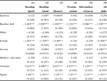
Willingness to pay regression results.

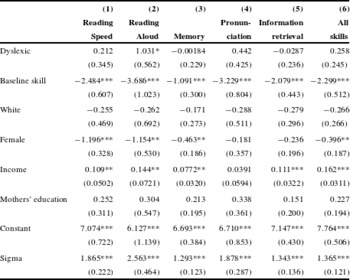
Notes: All regressions are maximum likelihood estimates. Dependent variable is log WTP for indicated skill. Regressions follow from equation (8). Robust standard errors are in parentheses: * significant at 10%, ** significant at 5%, *** significant at 1%.
Table 6 reports estimates of the WTP equation described in equation (8), calculated separately for each of the six interventions and correcting for the time costs of participating in the training sessions.Footnote 5 The dependent variable in each regression is the natural logarithm of WTP in 2005 dollars. Estimates are obtained using full-information maximum likelihood. For all skills (i.e., columns), WTP is negatively and significantly associated with baseline skill level; i.e., individuals with lower baseline skills value improvement more than other individuals. Controlling for baseline skill, individuals with dyslexia value improvements in reading aloud more than individuals without dyslexia, but there is no significant difference for other skills. Women have significantly smaller WTP than men for improvements in reading speed, reading aloud, memory, and all skills jointly. The estimated coefficients on income are positive and, except for pronunciation, significantly different from zero. Normally, a positive relationship between WTP for a good and income is expected. Finally, we find no significant effects of mothers’ education on WTP for any skill improvement.
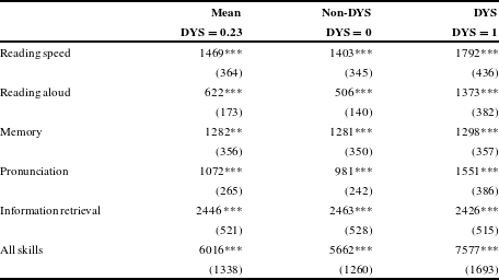
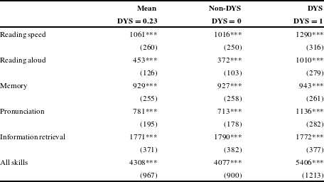
Our WTP questions elicit the value of improving skills up to a subjective level categorized as “very good.” Our setting did not allow for exogenous changes in the baseline skill levels. Hence we cannot disentangle the effects of baseline skill and the magnitude of improvement. This limitation can be overcome by estimating marginal WTP at zero improvement using equation (5). The numerator in equation (5) coincides with our identified effect and includes the joint effects of baseline skill level and improvement on WTP. MWTP calculated from equation (10) estimates the individual’s MWTP at zero skill improvement. These values are measured as dollars for a unit change in normalized skill (i.e., from “very bad”
 $=$
0 to “very good”
 $=$
1) and are reported in Table 7. Average MWTPFootnote
6
for an improvement in skill ranges from $600 dollars for the reading aloud intervention to $2400 for the information retrieval intervention. The values are in general larger for dyslexic than for nondyslexic respondents, significantly so only for reading aloud.Footnote
7
Marginal willingness to pay for improvement intervention.

Notes: MWTP is calculated using equation (10) for the sample-mean respondent, except DYS
 $=$
0 or 1 as shown. Log WTP is transformed to dollars by exponentiation (hence the estimate is the median over the error term). Robust standard errors are in parentheses: * significant at 10%, ** significant at 5%, *** significant at 1%.
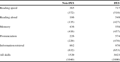
WTP to improve skill to a “very good” level can be estimated as the product of the potential skill improvement (Table 2) and the MWTP for that skill (Table 7). These values are shown in Table 8.Footnote 8 Although the estimated MWTP for skill improvement is generally similar for dyslexic and nondyslexic individuals, the potential skill improvement is larger for dyslexics and hence WTP for the incremental improvement that was elicited in our survey is also larger. Total WTP to improve all five skills jointly is approximately twice as large for dyslexic as for nondyslexic respondents (a difference of $1500); the largest proportional difference (a factor of five) is for reading aloud. In contrast, total WTP to improve memory and information retrieval is similar, as the differences in reported levels of these skills are modest.
Total WTP to improve skills to “very good.”

Notes: Estimated WTP to improve self-reported skill level from current level to “very good.” Calculated as the product of self-reported skill improvement (Table 2) and marginal WTP for improvement (Table 7). Standard deviations calculated assuming estimates of skill improvement and of MWTP are independent.
5 Validity and robustness tests
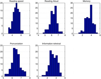
When one desirable good is nested within (is a proper subset of) another, the larger good should be valued at least as much as the smaller good (Hanemann, Reference Hanemann1994). Our results are consistent with this hypothesis as MWTP for an intervention improving all five skills jointly is larger than MWTP to improve any single skill (Figure 1). Nondyslexic respondents’ MWTP averages between $500 and $2500 for improvement of a single skill and about $5700 for improvement of all five skills jointly. Dyslexic respondents’ MWTP is larger: between $1300 and $2400 for improvement of a single skill and about $7600 for an improvement of all five skills jointly.
Willingness to pay to improve all skills jointly compared with improving single skill. The figure displays the distribution of
 $t$
-values from 100 replications. We divide the population into random subsamples 100 times. For each replicate, we run five regressions similar to those in Table 6 but including an additional variable coded 1 for respondents in one subsample (who value all interventions simultaneously) and 0 for respondents in the other subsample (who value a single skill). The regression model is:
 $C_{it}(e,w,s)=\unicode[STIX]{x1D6FC}_{1}All_{i}+x_{i}\unicode[STIX]{x1D6FD}+\unicode[STIX]{x1D709}+\unicode[STIX]{x1D716}_{it}$
, where
 $All_{i}$
is equal to 1 if respondent
 $i$
belongs to the subsample answering the question concerning an increase in all skills and 0 otherwise,
 $x_{i}$
represents demographic variables,
 $\unicode[STIX]{x1D709}$
is a constant term, and
 $\unicode[STIX]{x1D716}_{it}$
rationalizes idiosyncratic unobserved variation. Over all replications, coefficient
 $\unicode[STIX]{x1D6FC}_{1}$
was positive and mean values (standard deviations) were 1.14 (0.20), 1.78 (0.24), 0.67 (0.16), 1.74 (0.24) and 0.61 (0.20) for reading speed, reading aloud, memory, pronunciation and information retrieval, respectively.

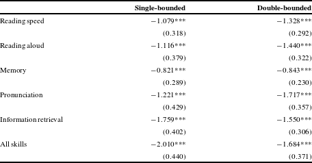
We elicited WTP for skill improvements using a double-bounded binary-choice format. The initial bid is exogenous but the follow-up bid is not (Cameron & Quiggin, Reference Cameron and Quiggin1994). The probability of receiving a follow-up bid larger than the initial bid corresponds to the probability that the respondent answers “yes” to the first bid. The endogeneity of the second bid could bias our estimates. As a robustness check, we compare the coefficients estimated using only the first bids to the standardized coefficients from our double-bounded binary-choice setting.
Validity test: Single-bounded vs. double-bounded estimates.

Notes: All regressions use maximum likelihood estimation. Dependent variable is log WTP for indicated skill. Regressions follow from equation (8). Single-bounded estimates are from a probit equation, assuming the residual variance equals one. Double-bounded estimates correspond to the estimates reported in Table 6 divided by the estimated standard deviation of the error (sigma). Robust standard errors are in parentheses: * significant at 10%, ** significant at 5%, *** significant at 1%.
In Table 9, we report the single-bounded and the double-bounded estimates for the WTP equation described in equation (8), estimated separately for each of the five interventions. Because the initial bid was common across respondents, single-bounded estimation corresponds to a probit model. Without variation among our initial bids we cannot identify the scale of the WTP distribution from the coefficients using a standard probit (we follow the usual identification assumption of normalizing the variance of the residual error to one). To compare coefficient estimates between the double-bounded and single-bounded estimates, we divide the estimated coefficients of the double-bounded estimates by the standard deviation (scale) of the WTP distribution estimated from that equation. All specifications include the same independent variables as in Table 6, though we report only the coefficients for baseline skill. The estimated coefficients from the single- and the double-bounded frameworks are quite similar, suggesting that endogeneity of the second bids does not substantially bias our estimates.
6 Discussion and conclusions
We find that both dyslexic and nondyslexic individuals value improvements in a variety of reading, speaking, and cognitive skills. Marginal WTP for individual skills ranges from $500 to $2500 for nondyslexic individuals and somewhat more, from $1300 to $2400 for dyslexic individuals (these values include the imputed costs of participating in 16 hours of training sessions). The between-group difference in MWTP is not statistically significant except for reading aloud. Because dyslexics have lower self-reported skills than nondyslexics, their total WTP for an improvement to a “very good” level is larger. In both groups, MWTP for a program to enhance all five skills simultaneously is significantly larger than MWTP for each single skill, which provides some evidence that these results can be interpreted as valid estimates of preferences. As is true with any stated-preference study, we cannot exclude the possibility that our estimates of WTP are biased downward if some respondents do not believe the interventions described would yield the stated improvements. This possibility could also affect the estimated difference in MWTP between dyslexic and nondyslexic individuals.
Our estimates of dyslexic individuals’ WTP for improvements in these skills are smaller than the difference in earnings between dyslexic and nondyslexic adults. For example, dyslexic respondents’ average WTP to improve all skills jointly to “very good” is estimated to be $3000; in contrast, we estimate that dyslexic individuals may earn 15% less per year (about $8000) than nondyslexic individuals.Footnote 9 How should this difference be interpreted?
WTP for an intervention at age 33 to improve reading, speaking, or cognitive skills should logically include the effects on future earnings and on other contributors to wellbeing. The earnings difference observed at age 33 results from differences in educational attainment, early work experience, and other factors between dyslexic and nondyslexic individuals; an improvement in skills at middle age is unlikely to shift dyslexic individuals to the earnings trajectory they would have followed if their skills had been improved as children. In addition, WTP should include only the individual’s (post-tax) share of the earnings increase. Hence, it would be unsurprising if the contribution of the interventions to future earnings were substantially smaller than the observed earnings differential. However, WTP should also include the value of skill improvement to other aspects of wellbeing, such as reading for pleasure or avoiding aggravation or embarrassment when unable to remember a name or pronounce it correctly. This component would be additional to the effect on future earnings. It is difficult to assess its potential magnitude. The absence of a significant difference in life satisfaction between dyslexic and nondyslexic individuals suggests it may be modest, though life satisfaction may not be a sufficiently sensitive measure to detect the difference. In summary, we suspect that stated-preference estimates of reading, speaking, and cognitive skills may substantially underestimate the value of these skills.
Acknowledgments
We thank Glenn Blomquist and the two anonymous reviewers for extremely helpful comments. We also thank supporters of the Connecticut Longitudinal Study: Connecticut State Department of Education; U.S. Department of Education; U.S. National Institutes of Health; and Seedlings Foundation.
Author information
The authors declare no competing financial interests.
Appendix
Willingness to pay regression results without time cost.

Marginal willingness to pay for improvement intervention without time cost.

To derive equation (5) we take equation (3),
 $$\begin{eqnarray}\displaystyle \frac{\unicode[STIX]{x2202}C}{\unicode[STIX]{x2202}s}=\frac{\displaystyle \frac{\unicode[STIX]{x2202}U}{\unicode[STIX]{x2202}s}}{\displaystyle \frac{\unicode[STIX]{x2202}U}{\unicode[STIX]{x2202}w}}-\frac{\displaystyle \frac{\unicode[STIX]{x2202}u}{\unicode[STIX]{x2202}s}}{\displaystyle \frac{\unicode[STIX]{x2202}U}{\unicode[STIX]{x2202}w}}, & & \displaystyle \nonumber\end{eqnarray}$$
and we replace the first term on the RHS using equation (2) which yields:
 $$\begin{eqnarray}\displaystyle \frac{\unicode[STIX]{x2202}C}{\unicode[STIX]{x2202}s}=\frac{\unicode[STIX]{x2202}C}{\unicode[STIX]{x2202}e}-\frac{\displaystyle \frac{\unicode[STIX]{x2202}u}{\unicode[STIX]{x2202}s}}{\displaystyle \frac{\unicode[STIX]{x2202}U}{\unicode[STIX]{x2202}w}}. & & \displaystyle \nonumber\end{eqnarray}$$
Next we multiply and divide the second term on the RHS by the marginal utility in case of no skill improvement and obtain,
 $$\begin{eqnarray}\displaystyle \frac{\unicode[STIX]{x2202}C}{\unicode[STIX]{x2202}s}=\frac{\unicode[STIX]{x2202}C}{\unicode[STIX]{x2202}e}-\frac{\displaystyle \frac{\unicode[STIX]{x2202}u}{\unicode[STIX]{x2202}s}}{\displaystyle \frac{\unicode[STIX]{x2202}u}{\unicode[STIX]{x2202}w}}\frac{\displaystyle \frac{\unicode[STIX]{x2202}u}{\unicode[STIX]{x2202}w}}{\displaystyle \frac{\unicode[STIX]{x2202}U}{\unicode[STIX]{x2202}w}}\equiv \frac{\unicode[STIX]{x2202}C}{\unicode[STIX]{x2202}e}-\frac{\unicode[STIX]{x2202}C(0,w,s)}{\unicode[STIX]{x2202}e}\frac{\displaystyle \frac{\unicode[STIX]{x2202}u}{\unicode[STIX]{x2202}w}}{\displaystyle \frac{\unicode[STIX]{x2202}U}{\unicode[STIX]{x2202}w}}, & & \displaystyle \nonumber\end{eqnarray}$$
which implies:
 $$\begin{eqnarray}\displaystyle \frac{\unicode[STIX]{x2202}C(0,w,s)}{\unicode[STIX]{x2202}e}=\frac{\displaystyle \frac{\unicode[STIX]{x2202}C}{\unicode[STIX]{x2202}s}-\frac{\unicode[STIX]{x2202}C}{\unicode[STIX]{x2202}e}}{-\frac{\displaystyle \frac{\unicode[STIX]{x2202}u}{\unicode[STIX]{x2202}w}}{\displaystyle \frac{\unicode[STIX]{x2202}U}{\unicode[STIX]{x2202}w}}}. & & \displaystyle \nonumber\end{eqnarray}$$
Solving equation (4) for the denominator on the RHS and substituting the result yields:
 $$\begin{eqnarray}\displaystyle \frac{\unicode[STIX]{x2202}C(0,w,s)}{\unicode[STIX]{x2202}e}=\frac{\displaystyle \frac{\unicode[STIX]{x2202}C}{\unicode[STIX]{x2202}e}-\displaystyle \frac{\unicode[STIX]{x2202}C}{\unicode[STIX]{x2202}s}}{1-\displaystyle \frac{\unicode[STIX]{x2202}C}{\unicode[STIX]{x2202}w}}. & & \displaystyle \nonumber\end{eqnarray}$$