







1. Introduction
To mitigate the environmental impact of aircraft, such as fuel consumption, greenhouse gas emissions and noise pollution, novel propulsion systems are under exploration (Bonet et al. Reference Bonet, Schellenger, Rawdon, Elmer, Wakayama, Brown and Guo2011; Müller et al. Reference Müller, Heinze, Kožulović, Hepperle and Radespiel2014; Ahmed et al. Reference Ahmed, Zaman, Rezgui and Azarpeyvand2024). One solution is the over the wing (OTW) design, where the propeller is mounted at the trailing edge of the wing (Johnson & White Reference Johnson and White1986), which offers promising advantages such as a high lift-to-drag ratio and low flyover noise (Marcus et al. Reference Marcus, de Vries, Kulkarni and Veldhuis2018). However, drawbacks such as reduced propulsive efficiency compared with tractor configurations and an increased nose-down thrust-induced pitching moment have been identified (Veldhuis Reference Veldhuis2005). A proposed solution to these challenges is the distributed propulsion of small OTW rotors, as explored by De Vries, Brown & Vos (Reference De Vries, Brown and Vos2019) and Upadhyay & Zaman (Reference Upadhyay and Zaman2021). Nevertheless, there is still a high risk of potential flow separation (Roosenboom, Heider & Schröder Reference Roosenboom, Heider and Schröder2009) due to added adverse pressure gradients (APGs) provided by both the slipstream contraction of the wake behind the propeller and by the motion of the wall-bounded tip vortices. Recent studies (Lignarolo et al. Reference Lignarolo, Ragni, Scarano, Ferreira and Van Bussel2015; Dghim, Ferchichi & Fellouah Reference Dghim, Ferchichi and Fellouah2020; de Vries et al. Reference de Vries, van Arnhem, Avallone, Ragni, Vos, Eitelberg and Veldhuis2021; Di Felice et al. Reference Di Felice, Capone, Romano and Pereira2023; Hodgkin, Deskos & Laizet Reference Hodgkin, Deskos and Laizet2023) have focused on the turbulence of the wake behind the rotors and the effects of the boundary layer and separation on the aircraft performance. However, there is very limited information on the effects of the tip vortex and rotor wake on the structure of the turbulent boundary layer (TBL). In this work we explore these vortex/boundary-layer interactions through experiments and present our observations on the changes to the turbulent boundary-layer structure for different scenarios, especially focusing on the effects of propeller tip vortices embedded within the boundary layer.
In the literature, irrotational free stream with concentrated vorticity is a commonly studied phenomenon in external aerodynamics, observed in various scenarios such as vortices from the tips of an airfoil as noted by Harvey & Perry (Reference Harvey and Perry1971), vortex pairs impinging on free surfaces discussed by Lugt & Ohring (Reference Lugt and Ohring1992), helicopter blades during dynamic stall investigated by Carr (Reference Carr1988) and further elaborated by Leishman & Bagai (Reference Leishman and Bagai1998), and several others including shedding from stationary bluff bodies (Bearman Reference Bearman1984), hairpin type vortices in the turbulence production in boundary layers (Robinson Reference Robinson1991), wake of wind and tidal turbines (Cotroni et al. Reference Cotroni, Di Felice, Romano and Elefante2000; Schreck Reference Schreck2008; Di Felice et al. Reference Di Felice, Capone, Romano and Pereira2023; Hodgkin et al. Reference Hodgkin, Deskos and Laizet2023), propeller wake interaction with a wing (Muscari, Dubbioso & Di Mascio Reference Muscari, Dubbioso and Di Mascio2017; Felli Reference Felli2021) and wingtip vortex under the effect of a synthetic jet actuation (Dghim et al. Reference Dghim, Ferchichi and Fellouah2020). The main dynamics of the vortex interaction with the surrounding flow can be illustrated taking the case of the wake of a single rotor as an example. As explored in various studies including Lignarolo et al. (Reference Lignarolo, Ragni, Scarano, Ferreira and Van Bussel2015), there is a notable change in circulation along the span of the blades. This change generates a sheet of trailing vorticity that rolls up into tip vortices in the wake of a TBL, forming a helical system (Okulov et al. Reference Okulov, Kabardin, Mikkelsen, Naumov and Sørensen2019) that is a key characteristic in the wake instability studies on wind turbines.
When these wake vortices are shed near a wall, they either generate a boundary-layer flow or there is an interaction with the existing boundary layer. In unsteady boundary-layer flows produced by a vortex motion on a wall plane within an otherwise stagnant fluid (Peridier, Smith & Walker Reference Peridier, Smith and Walker1991), the vortex generates local APGs that then lead to zones of recirculation near the wall. This phenomenon is an example of unsteady boundary-layer separation, where the wall layer breaks down intermittently into several eruptions. Near separation, the displacement thickness ( $\delta ^{*}$) increases exponentially and wall shear stress (
 $\tau _{wall}$) goes to zero. Since unsteady boundary layers involve a diverse array of complex phenomena, the traditional criteria of
 $\tau _{wall} = 0$ and the onset of reverse flows are not sufficient to describe all cases of unsteady separation of laminar boundary layers. Sears & Telionis (Reference Sears and Telionis1975) demonstrated that at the point of zero shear stress, fluid particles are compressed in the tangential direction and elongated in the wall-normal direction; this process concentrates the vorticity into a narrow spike that moves away from the wall, as also described by Van Dommelen & Shen (Reference Van Dommelen and Shen1982). This is the dynamic process that occurs prior to separation in vortex-induced laminar boundary layers.
Previous work has extended these vortex/boundary-layer interactions to scenarios where there is an oncoming/pre-existing boundary layer, with studies by Sengupta, De & Sarkar (Reference Sengupta, De and Sarkar2003) examining the interaction between incompressible flat plate shear layers and convecting vortices. Such interactions destabilize the wall-bounded flow, potentially leading to unsteady separation due to the vortex-induced flow instabilities and the coupling between the vortex outside the TBL and the unsteady gradients of vorticity inside the boundary layer. As demonstrated by Doligalski & Walker (Reference Doligalski and Walker1984) and Chuang & Conlisk (Reference Chuang and Conlisk1989), a rectilinear vortex can therefore generate reverse flow depending on the relative velocities, producing pressure fluctuations on the wall and turbulence kinetic energy (TKE) in the boundary layer. This phenomenon is further elaborated in three-dimensional (3-D) vortex-surface interactions by Pedrizzetti (Reference Pedrizzetti1992), noting that vortices in proximity to the wall expose the boundary layer to APG and unsteady separation, a situation that is quite common in modern aircraft and requires further investigation to understand the complex flow topologies and eventual separation mechanisms. Similar outcomes are underlined in the work of Doligalski, Smith & Walker (Reference Doligalski, Smith and Walker1994), which delves into understanding the viscous response when a vortex is in proximity to a wall at high Reynolds numbers (Re). The work reveals, yet again, that a sequence of events transpires, culminating in an abrupt eruption, i.e. separation, which leads to the formation of new vortices. This phenomenon is further compounded by APGs within the frame of reference moving with the vortex. The quest to understand the phenomena that induce unsteady flow separation stems from its significant implications in various applications, notably in the efficiency of propellers within hybrid-electric propulsion systems. This interest is driven by the fact that separation results in a decrease in lift, impacting the overall performance of such systems.
The presence of a TBL with embedded streamwise vortices is of significant interest in engineering applications, such as in gas turbines, where streamwise vortices can damage the blades due to increased heat transfer between the hot gas and cooled blades. Overlooking their presence could result in substantial errors in design. Experiments aim to enhance our understanding of these phenomena and how to accurately model them numerically (Liu, Piomelli & Spalart Reference Liu, Piomelli and Spalart1996). The complexity of the phenomenon is further illustrated by Murray et al. (Reference Murray, Devenport, Alexander, Glegg and Wisda2018), who examines the effects of rotor proximity to the wall, leading to increased APG and 3-D effects that result in an unsteady separation beneath the rotor, which sources additional tonal noise at high thrust. This is compounded by the variation of the loading distribution along the blades, causing slipstream deformation, a phenomenon investigated by Marcus et al. (Reference Marcus, de Vries, Kulkarni and Veldhuis2018). The dynamics of flow separation, especially with the introduction of a flap mechanism and the impact of external APG on the TBL, are further elucidated by de Vries et al. (Reference de Vries, van Arnhem, Avallone, Ragni, Vos, Eitelberg and Veldhuis2021), showing that APG are stronger with small tip clearances and higher thrust. This interaction deforms the tip vortices, shifting them towards the wall and altering the net forces acting on them, ultimately leading to flow separation, as the vortices split in two halves and are convected downstream, causing pressure fluctuations OTW. Therefore, the presence of APG weakens the TBL, and the presence of tip vortices generates velocity deficits and pressure perturbations within the TBL, leading to flow separation. This understanding prompts the suggestion to move the propeller upstream to avoid separation through the Coanda effect, a strategy supported by the observations of vortices being shed inside a TBL.
When a single vortex is introduced into a TBL with a zero pressure gradient (ZPG) and operates at a low speed, it induces negative Reynolds shear stress within the core of the vortex and alters the spanwise wall shear stress, diverging from what is typically observed over a flat plate (Shabaka, Mehta & Bradshaw Reference Shabaka, Mehta and Bradshaw1985). Furthermore, the introduction of two counter-rotating vortices, either in configurations where their common flows are upward or downward (Mehta & Bradshaw Reference Mehta and Bradshaw1988; Pauley & Eaton Reference Pauley and Eaton1988; Cutler & Bradshaw Reference Cutler and Bradshaw1989), significantly distorts the TBL. This results in modifications to skin friction and Reynolds stresses that display 3-D characteristics. In these scenarios, the velocity profiles also markedly deviate from a ‘standard’ boundary layer. The turbulent transport within the upwash region of the vortex pair is crucial for the generation of TKE, while the mean velocity gradients are instrumental in producing  $\langle uv\rangle$ throughout the TBL (Liu et al. Reference Liu, Piomelli and Spalart1996). An in-depth analysis aimed at elucidating the mechanisms that govern Reynolds stresses is essential. This would enable comprehensive analysis of transport equations and facilitate improvements in Reynolds stress models.
By and large, the following questions on vortex/boundary-layer interactions remain unanswered.
(i) What implications arise when the vortices rotate in the spanwise direction through an helicoidal pattern and are advected by the flow within a TBL? A partial answer has been given by de Vries et al. (Reference de Vries, van Arnhem, Avallone, Ragni, Vos, Eitelberg and Veldhuis2021), but no information is provided on the turbulence mechanisms and skin friction development inside the boundary layer.
(ii) Does the vertical position of these vortices (i.e. within the log region or further away) have an impact on the mean flow and the turbulence statistics of the boundary layer?
(iii) How are flow motions within the boundary layer organized under these conditions?
This study attempts to address these questions by presenting some experimental observations on the organization of a TBL in the wake of a two-blade propeller. This results in an interaction between a sequence of embedded spanwise vortices and the boundary layer. By means of a triple decomposition of the flow fluctuations, the effects on the turbulent stresses of the periodic flow structures generated by the rotation of the propeller are investigated separately from the effects of the background turbulence. We utilize two-point spatial correlation to analyse the phase-locked structures that emerge from the interaction between the tip vortex and the boundary layer. Additionally, turbulence production in both periodic and random fluctuations and viscous dissipation are evaluated for the two different blade tip clearances.
2. Experimental methodology
The experiments were conducted in the boundary-layer wind tunnel (BLWT) located at the University of Southampton. The BLWT is a ‘Göttingen’-type closed wind tunnel with a 12 m long test section. The inner cross-section of the test section measures  $1.2 \ \text {m} \times 1\ \text {m}$. The test section is divided into five segments, each spanning 2.4 m. To maintain a controlled environment, the temperature within the test section is maintained at
 $20^\circ$ using a cooling unit. The free-stream turbulence intensity is below 0.1 %. The wind tunnel is equipped with acrylic windows, thereby allowing optical access for particle image velocimetry (PIV) experiments. At the inlet of the test section, a zigzag strip is positioned to induce a laminar-to-turbulent transition. At the measurement station (8.4 m downstream of the trip), the velocity profile was examined using hot-wire anemometry (Wangsawijaya, Jaiswal & Ganapathisubramani Reference Wangsawijaya, Jaiswal and Ganapathisubramani2023) that showed a TBL, characterized by a thickness,
 $\delta _0$, of 11.6 cm (at a free-stream speed of
 $16\ {\rm m}\ {\rm s}^{-1}$). For further details on the TBL and its characterization into the BLWT, please refer to Ferreira, Costa & Ganapathisubramani (Reference Ferreira, Costa and Ganapathisubramani2024) and Wangsawijaya et al. (Reference Wangsawijaya, Jaiswal and Ganapathisubramani2023).
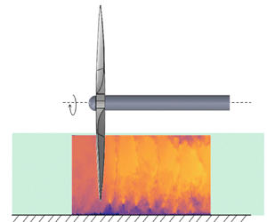
A two-bladed plastic drone propeller, with a 16 inch diameter and 5.5 inch pitch, manufactured by APC was chosen for this study (see figure 1). Similar to a real OTW application, the propeller diameter was selected to be larger than the boundary-layer thickness, so to have  $D=3.5\times \delta _0$. This choice was made in order to have the position of the hub as far as possible from the outer region of the TBL. To minimize reflections during PIV measurements, the propeller was painted black. A U7-V2.0 KV280 model from T-motor was used to drive the propeller and it was controlled by a Master Mezon 135 opto unit (ESC) power supply. The propeller was securely mounted on the fourth segment of the test section, positioned 8.4 m downstream from the test section inlet. This is the same position where a canonical boundary layer of a flat plate was characterized at the same free-stream velocity. To mitigate any flow-induced vibrations originating from the support structure, a wing with a NACA0030 airfoil profile was strategically placed more than one diameter away from the propeller. Additionally, a clearance of more than one diameter was maintained between the propeller tip and the tunnel windows and ceiling to avoid wall effects. The propeller was mounted in the set-up such that the distance between the rotor and the wind tunnel floor (i.e. tip clearance,
 $\varepsilon$) could be altered. To investigate the impact of the ingesting propeller on the TBL, two different tip clearances were examined, which are
 $\varepsilon = 1\ \text {cm}$ and
 $\varepsilon = 6\ \text {cm}$, corresponding to
 $\varepsilon /\delta _0 = 0.1$ and
 $\varepsilon /\delta _0 = 0.5$, respectively.
Two-blade propeller mounted inside the test section of the 12 m long boundary-layer wind tunnel (University of Southampton). (a) Region of interest: in green, the laser sheet shot from downstream the test section;  $\epsilon$ is the tip clearance;
 $\delta _0$ is the thickness of the boundary layer; the numbered dashed boxes are the field of view of the three PIV cameras. (b) Schematics: (1) propeller, (2) airfoil, (3) load cell, (4) laser optics, (5) tachometer, (6) test section.

The forces were measured using an ATI Mini-45 six-degree-of-freedom force balance, while an ICP laser tachometer sensor was employed to determine the rotational speed of the propeller ( $\varOmega$). Prior to conducting any other measurements (such as rotational speed), the propeller was set to a known thrust value of
 $T = 10\ \text {N}$, which is a typical value for drone-sized vehicles. The
 $C_T$ values obtained with the selected thrust and motor speed are similar to those studied in the work of Marcus et al. (Reference Marcus, de Vries, Kulkarni and Veldhuis2018). This initial characterization of the propeller's performance was crucial before proceeding with flow field measurements. To obtain information on the corresponding rotational speed, both forces and tachometer signals were recorded for 30 s at a 10 kHz sampling rate. These measurements were taken for both tip clearances at a thrust of 10 N and a free-stream speed (
 $U_\infty$) of
 $16\ \text {m}\ \text {s}^{-1}$. Each case was repeated four times and the results were time averaged. The relative standard error in thrust force was found to be 1.8 % and 1.2 %, while for the rotational speed, it was 14 % and 6 % for
 $\varepsilon /\delta _0 = 0.1$ and
 $\varepsilon /\delta _0 = 0.5$ cases, respectively. The corresponding thrust coefficients (
 $C_T = {T}/{\rho \varOmega ^2 D^4}$, where
 $T$ is thrust,
 $\rho$ is the density of air,
 $\varOmega$ is rotational speed given in revolutions per second and
 $D$ is the diameter of the propeller) along with other test parameters (the tip speed to free-stream velocity ratio
 $\lambda$, blade passing frequency
 $f_{prop}=2\times \varOmega$ (2 being the number of blades) and TBL time scale
 $f_{TBL}=U_{\infty }/\delta _0$) are summarized in table 1.
Test matrix.

Low-speed high-resolution planar PIV measurements were conducted to capture the flow fields for the specified cases. The imaging set-up involved three 16 MP cameras (LaVision Imager ProLX) equipped with 105 mm lenses. A Litron Bernoulli PIV series laser (LPU550) and JEM pro-fog served as the light source and seeding fluid, respectively. The laser beam was directed using mirrors toward the propeller. Along the streamwise direction, a telescopic lens was positioned inside the tunnel. This arrangement not only compensated for the laser beam divergence but also ensured an appropriate beam thickness throughout the investigation region (approximately 1.5 mm). The beam then passed through a cylindrical lens with a focal length of  $f = -20\ \text {mm}$, illuminating the centreline and the lower half of the propeller (i.e. the region of interest). To trigger the system internally, we employed a LaVision programmable timing unit (PTU-X). For each case, 5000 images were sampled at a rate of 0.6 Hz. The low acquisition frequency was chosen to ensure minimally time-correlated measurement samples and to leverage the best beam quality that the laser could emit. The PIV acquisition was set at a maximum displacement of 15 pixels in the free stream and 5–6 pixels in the near wall region, particles diameter of 1–3 pixels, lenses with f-stop 1.8 and a depth of field of 2.5 mm. DaVis 8.4.0 served as the acquisition and processing software. To cross-correlate acquired images,
 $64 \times 64$ and
 $24 \times 24$ pixel interrogation windows were selected for the first and last passes with
 $50\,\%$ overlap. The resulting field of view was found to be
 $1.8D \times 0.35D$. The propeller's positioning allowed for
 $0.35D$ upstream and
 $1.5D$ downstream clearance. The spatial resolution achieved was 0.88 mm per final interrogation window, which in wall units correspond to
 $d^+=33$. The 50 % of overlap provides a vector spacing of
 $s^+=16.5$. The normalization in wall units is made with the friction velocity of the flow at
 $Re_x = 8.75\times 10^6$.
Due to the limitation of the tachometer's operation in the presence of the scattering of the particles in a confined space, an image processing technique was employed to determine the blade (phase) angle of the propeller, enabling subsequent phase locking of the measurements. Firstly, we captured the propeller's position at known phase angles (with  $5^\circ$ increments) before conducting the PIV runs. This calibration step provided essential information for calculating phase angles from instantaneous images. During the PIV experiments, acquired run images were processed to detect the blade's position and then compared with those obtained from the calibration images. It is important to note that this method for determining the propeller's phase is effective only when the propeller is within the field of view and oriented toward the cameras (foreside of the laser). Consequently, a constraint exists on the identifiable phase angles, corresponding to values between
 $\phi = 0^\circ$ and
 $\phi = 55^\circ$, where
 $\phi$ represents the angle formed between the vertical axis and the blade position within the plane perpendicular to the rotation axis of the propeller. Counterclockwise rotations are conventionally designated as positive. This image processing scheme allows us to phase lock angles within the aforementioned range of
 $5^\circ$.
3. Results
3.1. Mean flow and turbulence statistics
We first focus on the visualization and analysis of the tip vortices generated by the propeller's blades that interact with the wall boundary layer. The wall-normal-streamwise plane, in figure 2, captures the distinct trace of the helicoidal vortices produced by the two-blade propeller. Phase-averaged field analysis at  $\phi =0^\circ$ reveals that the decay of tip vortices is faster when the blades are mounted closer to the wall, as depicted in figure 2(a). The manifestation of tip vortices is profoundly affected by the wall-bounded turbulence within the boundary layer, and this influence varies with the tip clearance (
 $\epsilon$). Interestingly, at
 $\varepsilon /\delta _0=0.1$ and at a distance of
 $3.5\delta _0$ behind the propeller, the tip vortices undergo complete disruption (figure 2b), leading to the breaking of the helicoidal tip blade vortex. Our observations are in line with the work of de Vries et al. (Reference de Vries, van Arnhem, Avallone, Ragni, Vos, Eitelberg and Veldhuis2021) who demonstrate a similar vorticity interaction, describing the reasons for the significant downward displacement of the tip vortices. The viscous shear generated by this interaction is responsible for the varying forces applied to the tip vortices and their disruption. Conversely, when the tip clearance is comparably larger (i.e.
 $\varepsilon /\delta _0=0.5$), the decay is more gradual (figure 2d) and the interaction with the wall vorticity is notably absent.
Phase-locked mean flow field and vorticity at  $\phi =0^\circ$: (a,c) dimensionless streamwise velocity component; (b,d) dimensionless spanwise vorticity component; (a,b)
 $\varepsilon =0.1\delta _0$; (c,d)
 $\varepsilon =0.5\delta _0$; the region upstream of the blade is being masked due to the presence of its shadow during PIV measurements, which decreases the signal-to-noise ratio.

The propeller, acting as an energy source, imparts acceleration to the incoming boundary layer, reaching velocities up to 1.8 times that of the free stream (see figure 3a,c). Analysis of the mean flow behind the blades reveals a distinctive contraction in the slipstream tube generated by the propeller rotation, inducing local APGs and deceleration of the wall-bounded flow. The assumption of the pressure gradients as a consequence of the slipstream contraction behind the propeller is demonstrated experimentally by both Marcus et al. (Reference Marcus, de Vries, Kulkarni and Veldhuis2018) and de Vries et al. (Reference de Vries, van Arnhem, Avallone, Ragni, Vos, Eitelberg and Veldhuis2021), who measured a rise in the wall pressure coefficient immediately downstream of the propeller using an array of static pressure ports. Notably, there is no discernible evidence of flow separation in the mean flow. The creation of shear behind the blade tips is attributed to the tip vortices (shown in figure 2), which travel along the edge of the wall-bounded stream tube. Examining the boundary-layer profiles in figures 3(b) and 3(d), it becomes evident that in the presence of rotating blades, the flow behaves akin to being in an APG condition, with a reduction of wall-normal extent in the log region and an enhanced outer wake region. The values of the latter for both the tip clearances are shown in figure 4(b). The reduced extension of the logarithmic region in canonical boundary layers with APG was previously investigated by Monty, Harun & Marusic (Reference Monty, Harun and Marusic2011) who also showed that the wake region of APG boundary layers begins earlier, at  $y^+=150$ (
 $Re_{\tau }=2860, \beta =1.9$). The authors suggest that the reduced size of the log layer extension depends on both the
 $Re$ and the strength of the pressure gradient.
Axial mean flow and boundary-layer profiles: (a,c) dimensionless streamwise velocity component, (b,d) boundary-layer profiles in wall units, (a,b)  $\varepsilon =0.1\delta _0$, (c,d)
 $\varepsilon =0.5\delta _0$; red dashed line, log-law equation with values of k and B from Marusic et al. (Reference Marusic, Monty, Hultmark and Smits2013); circles, velocities in wall units; vertical dashed lines, streamwise positions of the blades’ tip in wall units; blue gradients from lighter to darker,
 $x/\delta _0=0.5$, 1, 1.5, 2.5, 3.5, 4.5; red circles, flat plate at
 $Re_{\theta }=12\,200$ (
 $Re_{\tau }=4400$). Due to the resolution of the PIV system, the mean velocity points shown in (b,d) below
 $y^+=30$ are not valid data.

Skin friction coefficient and wake parameter at different streamwise positions: (a)  $C_f = 2(u_\tau /U_\infty )^2$, (b)
 $\varPi$; black dot-dashed line,
 $C_f$ function of
 $Re_x$ for a smooth flat plate (Schlichting & Gersten Reference Schlichting and Gersten2016); red dashed line, position of the two-blade propeller; red circle, flat plate boundary layer (
 $C_f=0.0026$ and
 $\varPi =0.33$) at
 $Re_{\theta }=12\,200$ (
 $Re_{\tau }=4400$); crosses,
 $\varepsilon =0.1\delta _0$; circles,
 $\varepsilon =0.5\delta _0$; black, values of
 $C_f$ and
 $\varPi$ upstream of the propeller, at
 $x/\delta _0=-0.5$,
 $-1$; blue gradients from lighter to darker,
 $x/\delta _0=0.5$, 1, 1.5, 2.5, 3.5, 4.5.

To explore this further, the friction velocity  $u_{\tau }$ and the wake strength
 $\varPi$ are determined from the mean velocity profile using the method described by Rodríguez-López, Bruce & Buxton (Reference Rodríguez-López, Bruce and Buxton2015). The assumption validating the use of the aforementioned method relies on the existence of a limited portion of the boundary layer that adheres to the log-law function. In the presented tip vortices/TBL interaction, the boundary layer is disrupted by the movement of the tip vortices at each rotational phase of the blades. However, statistically speaking, by considering the ensemble of velocity fields at all phases
 $\phi$, a portion of the log layer remains intact. This is demonstrated in figures 3(b) and 3(d), where the extent of the log layer exists and particularly depends on
 $x/\delta _0$ and tip clearance. The procedure finds the optimum solution
 $\{u_{\tau }, \kappa, \delta, \varPi \}$ that minimizes the error between the measured mean velocity profile and the analytical functions, i.e.
 \begin{equation} U^+_{canonical} =\begin{cases} U_{musker} + U_{bump} + \dfrac{2\varPi}{\kappa} W, & 0 \leqslant y \leqslant \delta, \\ U_{\infty}, & \delta \leqslant y \leqslant \infty, \end{cases} \end{equation}
with
 \begin{equation} U_{musker} = U_{musker}(y^+, \kappa, s) \end{equation}
obtained from
 \begin{gather} \frac{{\rm d}U_{musker}}{{{\rm d}y}^+} = \frac{\dfrac{(y^+)^2}{k} + \dfrac{1}{s}}{(y^+)^3 + \dfrac{(y^+)^2}{k} + \dfrac{1}{s}} , \end{gather}
 \begin{gather}U_{bump} = U_{bump}(y^+) = \exp[-\log^2(y^+{/}30)]/2.85 , \end{gather}
 \begin{gather}W = W(y/\delta) , \end{gather}
 \begin{gather}B = B(\kappa) , \end{gather}
 \begin{gather}s = s(\kappa). \end{gather}
Equation (3.1) represents the analytical form used to describe the canonical flow from the inner layer to the log-law region. It also depends on  $s$, which is the constant relating the eddy viscosity in the inner and overlap regions. In fact,
 $U_{musk}$ takes into account a continuous change in the eddy viscosity from the wall to the overlap region, adapting the linear to the log region (Musker Reference Musker1979). Contrary,
 $U_{bump}$ does not depend on s and includes an overshoot over the log law onto the buffer layer, which is generally used for a better description of mean velocity profiles at high Re (Rodríguez-López et al. Reference Rodríguez-López, Bruce and Buxton2015). Equation (3.5) is the exponential wake function described in Chauhan, Monkewitz & Nagib (Reference Chauhan, Monkewitz and Nagib2009). During the optimization routine, the values of the von Kármán constants
 $\kappa$ and
 $B$ are kept fixed as in Chauhan et al. (Reference Chauhan, Monkewitz and Nagib2009), at values respectively of 0.39 and 4.2 as our aim is to explore the effects of the propeller wake on the boundary-layer state. This assumes that all velocity profiles will have a log region with differences exhibited only in the wall-normal extent compared with a canonical TBL. This choice allows for evaluating how propeller/boundary-layer interactions affect the outer region, and thus, the wake structure. Having said that, we also allowed
 $\kappa$ and
 $B$ as part of the optimisation and this did not show sufficient change in these values (relative to uncertainty). This further reinforces our approach of fixing these values and examining the differences in the resulting values of other quantities.
When the blade tips rotate within the log region of the TBL ( $\varepsilon =0.1\delta _0$, see figure 3b), the most significant deviation from the canonical case occurs at an axial distance of
 $x/\delta _0=0.5$ from the propeller. Subsequently, as the axial distance increases, the wake amplification diminishes and the log region gradually extends, signifying a partial recovery of the boundary layer towards its canonical state. Conversely, at a tip clearance of
 $0.5\delta _0$ (see figure 3d), the attenuation of the wake of the TBL profiles is less pronounced with
 $x/\delta _0$. All profiles behind the rotating blades collapse onto a single curve, indicating that a greater distance from the propeller is required to observe the damping effects of the wall on the tip vortices.
Upstream of the propeller, the flow adhering to the wall undergoes acceleration, resulting in a notable rise in skin friction (figure 4a). Immediately behind the propeller, within the zone marked by the contraction of the slipstream, local APGs emerge at the wall, causing a localized reduction in skin friction ( $C_f$) to its minimum (see figure 4a). This phenomenon is consistent for both tip clearances, with a more pronounced decrease observed when
 $\varepsilon =0.1\delta _0$. The proximity of the propeller to the wall intensifies the streamline contraction within the logarithmic region of the TBL (see figure 3a), concurrently amplifying the magnitude of the APG (Marcus et al. Reference Marcus, de Vries, Kulkarni and Veldhuis2018). In practical scenarios, the presence of a flap system at the airfoil's trailing edge can further amplify these APGs, potentially leading to flow separation, especially during short takeoffs (de Vries et al. Reference de Vries, van Arnhem, Avallone, Ragni, Vos, Eitelberg and Veldhuis2021). As the flow progresses downstream (towards
 $x/\delta _0=4.5$), a noteworthy trend emerges, wherein the skin friction coefficient (
 $C_f$ in figure 4a) experiences an increase. Values up to 1.3 times and 2 times larger than those observed in a canonical case are reached, respectively for tip clearances of
 $\varepsilon /\delta _0=0.5$ and 0.1. This suggests that the APG effects diminish with downstream distance and that the flow starts to feel the new ‘free stream’ where the flow is accelerated leading to higher skin friction.
Figure 5 compares the streamwise and wall-normal turbulent fluctuations at different axial distances from the propeller to the flat plate reference case for two different tip clearances. It appears that both streamwise and wall-normal fluctuations do not conform to local scaling (with  $u_\tau$) as the data do not exhibit collapse (for both values of
 $\epsilon$). This suggests that non-local flow parameters are required to capture the trends in turbulence statistics. This is analogous to history effects of pressure gradients where local
 $u_\tau$ does not necessarily collapse the data since the outer-layer large scales and the smaller scales nearer to the wall experience different effects. This needs further exploration in future work. Furthermore, the peak values and their wall-normal positions appear to depend on the axial distance (
 $x/\delta _0$) from the propeller position. With the scaling in wall units, as the streamwise distance (
 $x/\delta _0$) increases, the peaks of
 $u$ and
 $v$ fluctuations diminish (see figure 5). The same occurs particularly for the wall-normal statistics when scaling the data with the outer scale (see figure 6b,d). The dependence of the peak of the streamwise velocity fluctuations on
 $x/\delta _0$ is less evident if compared with the results in wall units (see figure 5a,c). When the tip clearance is small (
 $\varepsilon =0.1\delta _0$), specifically at
 $x/\delta _0=0.5$ behind the propeller, the
 ${\rm r.m.s.}(u)^+$ profile manifests a distinctive double-peak shape (see figure 5a). The same pattern is shown with the outer scaling of the flow statistics (see figure 6a,c). This is a consequence of the large scales generated by the rotation of the propeller at the height of the blade's tip. A similar trend is depicted in the work of Harun et al. (Reference Harun, Monty, Mathis and Marusic2013), where the impact of a mild APG on the large scales of a TBL was investigated. Subsequently, with an increase in
 $x/\delta _0$, these profiles transit to a single peak, which then progressively attenuates.
Root mean square of both axial and wall-normal fluctuations in wall units. Comparison at two different tip clearances: (a,b)  $\varepsilon =0.1\delta _0$, (c,d)
 $\varepsilon =0.5\delta _0$, (a,c) r.m.s. of
 $u$ in wall units, (b,d) r.m.s. of
 $v$ in wall units; circles, velocities in wall units; vertical dashed lines, streamwise positions of the blades’ tip in wall units; blue gradients from lighter to darker,
 $x/\delta _0=0.5$, 1, 1.5, 2.5, 3.5, 4.5; black circles, flat plate at
 $Re_{\theta }=12\,200$ (
 $Re_{\tau }=4400$).

Root mean square of both axial and wall-normal fluctuations in outer units. Comparison at two different tip clearances: (a,b)  $\varepsilon =0.1\delta _0$, (c,d)
 $\varepsilon =0.5\delta _0$, (a,c) r.m.s. of
 $u$, (b,d) r.m.s. of
 $v$; circles, velocities; vertical dashed line, streamwise positions of the blades’ tip; blue gradients from lighter to darker,
 $x/\delta _0=0.5$, 1, 1.5, 2.5, 3.5, 4.5; black circles, flat plate at
 $Re_{\theta }=12\,200$ (
 $Re_{\tau }=4400$).

The key disparity in assessing the effects of different tip clearances lies in the manifestation of the turbulence intensities. As shown by You et al. (Reference You, Wang, Moin and Mittal2007), the streamlines of the tip-gap flow experience a sudden change of directions along the span of the blade's tip, which generates spanwise derivatives of the mean  $U$ and
 $V$. When the propeller is mounted closer to the wall, the derivatives
 ${\partial U}/{\partial z}$ and
 ${\partial V}/{\partial z}$ increase in magnitude and so does the turbulent mixing. For
 $\varepsilon =0.1\delta _0$, the increase in turbulence intensities spans the entire log-law region and wake, commencing from
 $y^+=100$. In contrast, for the alternative tip clearance case (
 $\varepsilon =0.5\delta _0$), the effect is observed as a transient impulse of turbulent energy solely in the wake (see figure 5c,d). Importantly, the mean profile (and the log region) remains unaffected in this scenario. Crespo, Hernandez & Frandsen (Reference Crespo, Hernandez and Frandsen1999) reviewed different wake modelling methods for wind turbine farms design and defined the aforementioned localized peak of turbulence intensity seen at
 $\varepsilon =0.5\delta _0$ as ‘added turbulence’, i.e. the TKE added by the propeller locally to the periodic and random fluctuations at the blade tip's location.
3.2. Two-dimensional coherent structures
The spatial two-point correlation analysis of streamwise fluctuations (see figure 7) offers valuable insights into the coherent structures arising from the interaction between the propeller and the wall boundary layer. The two-point correlation coefficient between two velocity fluctuations  $R_{ij}$ is defined as in Ganapathisubramani et al. (Reference Ganapathisubramani, Hutchins, Hambleton, Longmire and Marusic2005), i.e.
 \begin{equation} R_{ij}(x,y) = \frac{\overline{u_i(x,y)u_j(x+\Delta x,y+\Delta y)}}{\sigma_i \sigma_j}, \end{equation}
where the overline notation is an ensemble average over multiple time realizations at all the angular positions of the blade,  $\sigma$ represents the standard deviation of the physical quantity and
 $(\Delta x, \Delta y)$ are the distances from the reference point
 $(x,y)$. Equation (3.8) is therefore a covariance of two fluctuating velocity components evaluated at two different points normalized in a way that
 $R_{ii}(0,0) = 1$. Conducted at six reference points spanning the entire axial distance within the field of view and fixed at both
 $y=0.1\delta _0$ for
 $\varepsilon =0.1\delta _0$ (figure 7a,c,e,g,i,k) and
 $\varepsilon =0.5\delta _0$ (figure 7b,d,f,h,j,l), and
 $y=0.5\delta _0$ for
 $\varepsilon =0.1\delta _0$ (figure 8a,c,e,g,i,k) and
 $\varepsilon =0.5\delta _0$ (figure 8b,d,f,h,j,l), this statistical tool reveals distinctive observations for different tip clearances.
Two-point correlation of streamwise fluctuations at several axial reference points  $y_{Ref}/\delta _0=0.1$: (a,c,e,g,i,k)
 $\varepsilon =0.1\delta _0$, (b,d,f,h,j,l)
 $\varepsilon =0.5\delta _0$, (a,b)
 $x/\delta _0=0.5$, (c,d)
 $x/\delta _0=1$, (e,f)
 $x/\delta _0=1.5$, (g,h)
 $x/\delta _0=2.5$, (i,j)
 $x/\delta _0=3.5$, (k,l)
 $x/\delta _0=4.5$, (a–l)
 $y/\delta _0=0.1$;
 $\Delta x/\delta _0=0$, x coordinate of the reference point.

Two-point correlation of streamwise fluctuations at several axial reference points with  $y_{Ref}/\delta _0=0.5$: (a,c,e,g,i,k)
 $\varepsilon =0.1\delta _0$, (b,d,f,h,j,l)
 $\varepsilon =0.5\delta _0$, (a,b),
 $x/\delta _0=0.5$, (c,d)
 $x/\delta _0=1$, (e,f)
 $x/\delta _0=1.5$, (g,h)
 $x/\delta _0=2.5$, (i,j)
 $x/\delta _0=3.5$, (k,l)
 $x/\delta _0=4.5$, (a–l)
 $y/\delta _0=0.1$;
 $\Delta x/\delta _0=0$, x coordinate of the reference point.

At  $\varepsilon =0.5\delta _0$, the coherent structure, captured at each different reference point, closely resembles those obtained in a flat plate boundary layer without pressure gradients. Their size and tilt angle are found to be respectively
 $(0.8 \pm 0.1)\delta _0$ and
 $(11.5 \pm 1)^\circ$, which closely match the values for the ZPG boundary layer reported in the work of Volino (Reference Volino2020) (for a ZPG,
 ${\rm size}=0.6\delta _0\unicode{x2013}1.0\delta _0$,
 ${\rm angles}=10^\circ \unicode{x2013}12^\circ$). The size of the coherent structures is measured as twice the maximum distance between the reference point of the two-point correlation and the isoline
 $R_{uu}=0.5$. In Volino (Reference Volino2020) it is shown that when the boundary layer is subjected to APGs, the streamwise length of the coherent structures shrink to
 $0.6\delta _0$ at angles up to
 $15^\circ$. Therefore, it can be inferred that in figures 7(b), 7(d), 7(f), 7(h), 7(j) and 7(l) there is little or insignificant influence of the rotating blades on the developing boundary layer in terms of velocity fluctuations, as their structure resembles that of a ZPG. Importantly, both the shape and intensity of coherency remain unaltered with the distance between the reference point and the propeller tip. By shifting the reference point further from the wall to
 $y/\delta = 0.5$, the shape of the correlation coefficient distribution (centred at
 $y_{Ref}$) changes, aligning the structures with the wall-normal direction (see figures 8 and 10). In figures 8(b), 8(d), 8(f), 8(h), 8(j) and 8(l), the size of the coherent structure, depicted by
 $R_{uu}$ and centred at the reference point, diminishes to
 $(0.4 \pm 0.1)\delta _0$. Notably, unlike in figures 7(b), 7(d), 7(f), 7(h), 7(j) and 7(l), where a single structure (as seen in canonical TBLs) is shown, several portions in the outer layer are correlated in the region
 $y > 0.3\delta _0$. Conversely, when the blades are in closer proximity to the wall (
 $\varepsilon =0.1\delta _0$), the two-point correlations behind the propeller unveil the generation of correlated and anti-correlated structures stacked in pairs (see figure 7a), which is consistent with the increased turbulence levels throughout the log region (see figure 5a,b). The vertical alignment of these structure pairs tilts with downstream distance (
 $x/\delta _0$), and beyond
 $2.5\delta _0$ from the propeller (see figure 7g), the coherence of these structures is disrupted. As the reference point moves downstream, the intensity of the two-point correlation structures diminishes, fading away at
 $4.5\delta _0$ from the tip of the blades. For longer distances, a single, smaller structure remains, weakly correlated to the outer region of the boundary layer. Interestingly, with a reference point at
 $y=0.5\delta _0$, a single large structure is observed, spanning the range
 $1.2 > y/\delta _0 > 0.2$, regardless of the axial distance chosen as a reference for the two-point correlation (see figure 8a,c,e,g,i,k). This implies that the outer region is more influenced by the wake of the propeller and less by the wall-bounded tip vortices.
Similar outcomes are observed in the two-point correlation analysis of wall-normal fluctuations (see figure 9), with the primary difference being the stretched wall-normal orientation of  $R_{vv}$ contours. This occurs only when the tip clearance is
 $\varepsilon =0.1\delta _0$, in the left column of figure 9, indicating that the wall/propeller interaction significantly influences the coherence of velocity fluctuations in the wall-normal direction throughout the developing boundary layer. For the larger tip clearance (
 $\varepsilon =0.5\delta _0$), the contours once again resemble that of a canonical boundary layer that does not seem to be influenced by the presence of the propeller. With the reference point at
 $y=0.5\delta _0$, the correlation patterns change slightly. At
 $\varepsilon =0.5\delta _0$ (see figure 10b,d,f,h,j,l), more structures are correlated in vertically oriented pockets of size
 $1\delta _0$, confined to the region
 $y > 0.3\delta _0$, and thus, do not affect the log layer of the TBL. In contrast, at
 $\varepsilon =0.1\delta _0$ (see figure 10a,c,e), the wall-normal oriented structures, centred at the reference point, are correlated with the wall-bounded structures behind the propeller over an extension of
 $\Delta x=2\delta _0$. In this case, the flow in the outer region impacts the wall-normal turbulence intensity more significantly compared with
 $\varepsilon =0.5\delta _0$.
Two-point correlation of wall-normal fluctuations at several axial reference points with  $y_{Ref}/\delta _0=0.1$: (a,c,e,g,i,k)
 $\varepsilon =0.1\delta _0$, (b,d,f,h,j,l)
 $\varepsilon =0.5\delta _0$, (a,b)
 $x/\delta _0=0.5$, (c,d)
 $x/\delta _0=1$, (e,f)
 $x/\delta _0=1.5$, (g,h)
 $x/\delta _0=2.5$, (i,j)
 $x/\delta _0=3.5$, (k,l)
 $x/\delta _0=4.5$, (a–l)
 $y/\delta _0=0.1$;
 $\Delta x/\delta _0=0$, x coordinate of the reference point.

Two-point correlation of wall-normal fluctuations at several axial reference points with  $y_{Ref}/\delta _0=0.5$: (a,c,e,g,i,k)
 $\varepsilon =0.1\delta _0$, (b,d,f,h,j,l)
 $\varepsilon =0.5\delta _0$, (a,b)
 $x/\delta _0=0.5$, (c,d)
 $x/\delta _0=1$, (e,f)
 $x/\delta _0=1.5$, (g,h)
 $x/\delta _0=2.5$, (i,j)
 $x/\delta _0=3.5$, (k,l)
 $x/\delta _0=4.5$, (a–l)
 $y/\delta _0=0.1$;
 $\Delta x/\delta _0=0$, x coordinate of the reference point.

Given that the structure of the fluctuations either conform to that of the boundary layer or that of the propeller wake, it is important to understand if the periodic velocity component from the propeller is a significant contributor to these fluctuations. This is explored in the next section.
3.3. Mechanics of the periodic motion
The triple decomposition methodology (Reynolds & Hussain Reference Reynolds and Hussain1972; Lignarolo et al. Reference Lignarolo, Ragni, Scarano, Ferreira and Van Bussel2015) serves as a valuable tool to disentangle the statistics of the fluctuations contributed solely by the periodic motions, generated through the rotation of the blades. The tool is capable of shedding light on the influence of the periodic motions on the background random fluctuations within the boundary layer. In general, according to the triple decomposition, a fluctuating velocity component can be divided into
 \begin{equation} u_i = \overline{u_i} + \tilde{u}_{i} + u_{s,i} , \end{equation}
where  $\overline {u_i}$ is the time-average contribution,
 $\tilde {u}_{i}$ is the periodic motion,
 $u_{s,i}$ is the background turbulent fluctuation of the signal and
 $i$ indicate the coordinate directions, with
 $i=1, 2$ corresponding to axial and wall-normal directions, respectively. The organized motion (
 $\tilde {u}_{i}$) is obtained by subtracting the time-average value (
 $\overline {u_i}$) from the phase average (
 $\langle u \rangle$), i.e. the conditional average over the points that have the same phase with respect to an oscillator, which in this case is the propeller:
 \begin{equation} \tilde{u}_{i} = \langle u_i \rangle - (\overline{u_i}) . \end{equation}
Effectively, the phase averaging of the velocity components allows rejecting the background turbulence nature of the field and extracting only the organized periodic motions from the signal (Reynolds & Hussain Reference Reynolds and Hussain1972).
Figure 11 provides a comprehensive analysis of the impact of the phase of the rotating propeller on the triple decomposed fluctuations. The investigation spans from  $0^\circ$, where the blades are perpendicular to the wall, to
 $50^\circ$ with an increment of
 $10^\circ$.
Phase-locked profiles behind the propeller ( $x=0.5\delta _0$) of both organized periodic and random fluctuations at two different tip clearances: (a,c,e,g)
 $\varepsilon =0.1\delta _0$, (b,d,f,h)
 $\varepsilon =0.5\delta _0$, (a,b)
 $\tilde {u}^+$, (c,d)
 $\tilde {v}^+$, (e,f) r.m.s. of
 $u_s^+$, (g,h) r.m.s. of
 $v_s^+$, (a–h)
 $x/\delta _0=0.5$; red dashed line, blades tip position in wall units at
 $\phi =50^\circ$; red gradients from darker to lighter,
 $\phi =0^\circ$,
 $10^\circ$,
 $20^\circ$,
 $30^\circ$,
 $40^\circ$,
 $50^\circ$; the velocity error estimation in wall units is
 $\varDelta ^+ = 0.25$.

At  $\varepsilon =0.1\delta _0$ (see figure 11a,c), the amplitude of the periodic motions is significant, affecting an extensive portion of the boundary layer. As the blade tip moves further away from the wall, the amplitude of
 $\tilde {u}$ and
 $\tilde {v}$ decreases. During the rotation from
 $\phi =0^\circ$, the blades draw the flow toward the wall-normal direction, diminishing the periodic fluctuations, which are particularly peaking at
 $\phi =10^\circ$ for
 $\tilde {u}$ and
 $\phi =0^\circ$ for
 $\tilde {v}$. Differently, at
 $\varepsilon =0.5\delta _0$ (see figure 11b,d), the trend is inverted. The amplitude of the periodic structures amplifies as the blade tip moves away from the wall (as
 $\phi$ increases from
 $0^\circ$ to
 $50^\circ$). Therefore, an initial observation can be made: with the rotating blades closer to the wall (
 $\varepsilon =0.1\delta _0$), the amplitude of the periodic motion (
 $\tilde {u}$ and
 $\tilde {v}$) is lowered as the angle of rotation
 $\phi$ increases, especially in the region of maximum slipstream contraction (
 $x=0.5\delta _0$). Further downstream (see figure 12a–d) for
 $x=2.5\delta _0$), the periodic features of the flow gets attenuated, when compared with figures 11(a)–11(d).
Phase-locked profiles behind the propeller ( $x=2.5 \delta _0$) of both organized periodic and random fluctuations at two different tip clearances: (a,c,e,g)
 $\varepsilon =0.1\delta _0$, (b,d,f,h)
 $\varepsilon =0.5\delta _0$, (a,b)
 $\tilde {u}^+$, (c,d)
 $\tilde {v}^+$, (e,f) r.m.s. of
 $u_s^+$, (g,h) r.m.s. of
 $v_s^+$, (a–h)
 $x/\delta _0=2.5$; red dashed line, blades tip position in wall units at
 $\phi =50^\circ$; red gradients from darker to lighter,
 $\phi =0^\circ$,
 $10^\circ$,
 $20^\circ$,
 $30^\circ$,
 $40^\circ$,
 $50^\circ$; the velocity error estimation in wall units is
 $\varDelta ^+ = 0.25$.

The periodic structures induced by the rotating blades exhibit a phase-driven movement, and their interaction with the mean flow contributes to the generation of background random fluctuations. At  $\varepsilon =0.1\delta _0$ (see figure 11e), the amplitude of the root-mean-square (r.m.s.) profiles of
 $u_{s}^+$ decreases with increasing angular position of the propeller. Conversely, the r.m.s. peaks of the wall-normal fluctuation
 $v_{s}^+$ profiles increase with the blade phase angle (see figure 11g). This suggests that at the smaller investigated tip clearance, the presence of the wall attenuates both the periodic and random fluctuations, with an exception for the wall-normal variance
 ${\rm r.m.s.}(v_s)^+$.
Further downstream from the propeller, at  $x=2.5\delta _0$ (see figure 12e,g), both the streamwise and wall-normal stochastic fluctuations of the flow, specifically at
 $\epsilon = 0.1\delta _0$, are not dependent on the angular rotation of the blades, whose amplitudes are much lower compared with
 $x=0.5\delta _0$ in figures 11(e) and 11(g). No anomalies are seen in this region due to the lack of slipstream/boundary-layer interaction. At
 $\varepsilon =0.5\delta _0$ (see figures 11f,h and 12f,h), the r.m.s. profiles of
 $u_{s}^+$ and
 $v_{s}^+$ behave in the same fashion with the angular phase, showing peak values at both
 $\phi =50^\circ$. Comparing these results with the statistics for the tip clearance case
 $\varepsilon =0.1\delta _0$, the portion of boundary layer affected by the interaction by the tip vortices is lower, extending from
 $y^+=2000$ to
 $y^+=6000$, ensuring that the log region of the boundary layer is not affected (contrary to the case
 $\varepsilon =0.1\delta _0$ where the tip-vortex influence extends down to
 $y^+=100$).
3.4. Phase-locked turbulent structures
The divergent trends observed in the angular phase of background fluctuations between the streamwise and wall-normal components at  $\varepsilon /\delta _0 = 0.1$ (figure 11e,g) suggest a distinct phenomenon, which becomes apparent as the blade tip diverges from the wall. These findings necessitate a further look at the turbulent flow structure at specific locations to explore the features that may be responsible for these statistics. The location of the slipstream contraction is a major factor that affects the observations in the previous section and, therefore, we examine two-point correlations of the random fluctuations at specific phases angles (of the propeller) in the vicinity of the slipstream.
Figure 13 provides an examination of coherent structures captured at different angular positions using two-point correlations, with reference points located at  $x/\delta _0=0.5$. The wall-normal reference is taken to be at the location of the slipstream (i.e.
 $y_{ref} = \epsilon$). The analysis focuses on fluctuations in the wall-normal direction only as these showed opposing trends to the streamwise fluctuations in the previous section. The analysis spans angular positions from
 $0^\circ$ (blade perpendicular to the wall) to
 $50^\circ$, with the effects beyond this range remaining unknown.
Two-point correlation of wall-normal fluctuations at phase-locked positions evaluated for two different tip clearances: (a,c,e,g,i,k)  $\varepsilon /\delta _0=0.1$, (b,d,f,h,j,l)
 $\varepsilon /\delta _0=0.5$. For all subfigures, (a–l)
 $x/\delta _0=0.5$: (a,b)
 $\phi =0^\circ$, (c,d)
 $\phi =10^\circ$, (e,f)
 $\phi =20^\circ$, (g,h)
 $\phi =30^\circ$, (i,j)
 $\phi =40^\circ$, (k,l)
 $\phi =50^\circ$; negative values of
 $R_{vv}$ filtered in (d,f,h,j,l) due to a lack of anti-correlated structures; the region upstream of the blade is being masked due to the presence of its shadow during PIV measurements, which decreases the signal-to-noise ratio; first column on the left, schematics of the phase-locked propeller positions, in the plane perpendicular to the flow (y–z).

For  $\varepsilon /\delta _0=0.5$ (see figure 13b,d,f,h,j,l), when the blade is perpendicular to the wall, an alternate arrangement of positive and negative correlation is observed behind the blade tip (figure 13b). The magnitude of correlation diminishes as the blade rotates away from the wall, suggesting that the tangential sweeping of the blades is not intense enough to impact the phase-locked ‘random’ vortices created by the interaction between the boundary layer and the propeller. As the blades rotate, they generate a swirling motion in their vicinity, adding a tangential component to the flow. Closer to a wall, along the height of the blade, spanwise derivatives of U and V are produced, becoming stronger near the wall (You et al. Reference You, Wang, Moin and Mittal2007). These stronger flow derivatives, which vary over time with the passage of the blades, enhance turbulent activity. Consequently, local random fluctuations depend on the phase position of the blade and the spanwise derivatives of the flow. Therefore, a decreased correlation
 $R_{ii}$ indicates that flow structures in that region fluctuate coherently with a lower intensity, as a result of the smaller magnitudes of the spanwise derivatives generated by the blades’ tangential motion. Conversely, for
 $\varepsilon /\delta _0=0.1$ (see figure 13a,c,e,g,i,k), when the blades are mounted closer to the wall, a different scenario is observed. As the blades rotate, the rotational effect amplifies the interaction between the propeller and the boundary layer. Coherent vortices behind the propeller exhibit strong correlation with absolute values that get close to unity. This is particularly evident in the train of vertical structures created by the propeller's rotation. These vertical and narrow regions in the flow field fluctuate with the same intensity in the wall-normal direction, becoming more pronounced as the blades move further from the wall.
In figure 14 the same correlation analysis is shown only for  $\varepsilon /\delta _0=0.1$, focusing on reference points at two streamwise positions:
 $x/\delta _0=1$ (see figure 14a,c,e,g,i,k) and
 $x/\delta _0=2.5$ (see figure 14b,d,f,h,j,l). This reveals that as the reference point moves downstream, the intense correlation values of the turbulent structures exhibit a modest increase with
 $x/\delta _0$ when compared with the
 $x/\delta _0=0.5$ case. It can be inferred that the presence of more intense coherent structures during the blades rotation is associated with a narrower contraction of the stream tube (at approximately
 $x/\delta _0=0.5$) and, consequently, with stronger APGs generated by the propeller itself. This suggests that the periodic motions generated by propeller rotation also generate corresponding turbulent fluctuations that remain in phase. Therefore, there should be a mechanism of energy transfer between the periodic motions to the random ones and this is explored further in the next section.
Two-point correlation of wall-normal fluctuations at phase-locked positions evaluated for  $\varepsilon /\delta _0=0.1$: (a,c,e,g,i,k)
 $x/\delta _0=1$, (b,d,f,h,j,l)
 $x/\delta _0=2.5$, (a,b)
 $\phi =0^\circ$, (c,d)
 $\phi =10^\circ$, (e,f)
 $\phi =20^\circ$, (g,h)
 $\phi =30^\circ$, (i,j)
 $\phi =40^\circ$, (k,l)
 $\phi =50^\circ$; the region upstream of the blade is being masked due to the presence of its shadow during PIV measurements, which decreases the signal-to-noise ratio; first column on the left, schematics of the phase-locked propeller positions, in the plane perpendicular to the flow (y–z).

3.5. Viscous dissipation and energy transfer
The triple decomposition method also allows further investigation of how the processes of energy transfer among mean flow, wave-induced and fluctuating fields take place. The travelling waves generated by the periodic motion of the propeller distort the surrounding turbulent field and interact distinctively with the boundary layer at different tip clearances. As a consequence, the altered energetic balance between dissipation into thermal energy, production and diffusion of turbulent kinetic energy can be assessed. The total time-averaged kinetic energy per unit mass at a specific point is
 \begin{equation} \tfrac{1}{2}
(\overline{u_i u_i}) = \tfrac{1}{2} \left( \bar{u_i}\,
\bar{u_i} + \overline{\tilde{u}_{i} \tilde{u}_{i}} +
\overline{u_{s,i} u_{s,i}} \right).
\end{equation}
The formulation for the second component of the kinetic energy on the right-hand side of (3.11) is obtained by first doing a phase averaging and then a time averaging of the momentum equation of the periodic motion multiplied by  $\tilde {u}_{\imath }$ (Reynolds & Hussain Reference Reynolds and Hussain1972):
 \begin{align} \frac{\bar{D}}{D
t}\left(\frac{1}{2} \overline{\tilde{u}_{\imath}
\tilde{u}_{\imath}}\right) &={-}\frac{\partial}{\partial
x_j}\left[\overline{\tilde{u}_{\jmath}\left(\tilde{p}+\frac{1}{2}
\tilde{u}_{\imath} \tilde{u}_{\jmath}\right)}\right]
\nonumber\\ & \quad + \left(-\overline{\tilde{u}_{\imath}
\tilde{u}_{\jmath}}\right) \frac{\partial
\bar{u}_{\imath}}{\partial x_j} -
\overline{\left(-\left\langle u_{s, \imath} u_{s, j}
\right\rangle\right) \frac{\partial
\tilde{u}_{\imath}}{\partial x_j}} \nonumber\\ & \quad
-\frac{\partial}{\partial
x_j}\overline{\left[\tilde{u}_i\left\langle u_{s, i} u_{s,
j}\right\rangle\right]} + \frac{1}{R e}
\frac{\partial}{\partial x_j}\left[\overline{\tilde{u}_i
\left(\frac{\partial \tilde{u}_t}{\partial
x_j}+\frac{\partial \tilde{u}_j}{\partial
x_i}\right)}\right] \nonumber\\ & \quad -\frac{1}{2 \,{Re}}
\overline{\left(\frac{\partial \tilde{u}_i}{\partial
x_j}+\frac{\partial \tilde{u}_j}{\partial
x_i}\right)\left(\frac{\partial \tilde{u}_i}{\partial
x_j}+\frac{\partial \tilde{u}_j}{\partial x_i}\right)} .
\end{align}
The right-hand side of (3.12) delineates the main components governing the net change rate of the kinetic energy content (left-hand side of (3.12)) of the organized periodic motions. The second and third terms on the right-hand side of (3.12) are the two most dominant entities affecting the energy balance. The second term,  $-\overline {(\tilde {u}_{i} \tilde {u}_{j})} (\partial (\overline {u_i})/\partial x_j)$, represents the turbulent production due to the action of the mean flow on the Reynolds stresses of the periodic motion generated by the rotation of the blades. Thus, it represents the amount of energy drained from the mean flow to produce turbulence in the periodic organized field. The third term,
 $-(-\overline {\langle u_{s,i} u_{s,j} \rangle (\partial \tilde {u_i}/\partial x_j)})$, is a drain of turbulent energy due to the interaction between the wave field and the Reynolds stresses of the background turbulence. The statistical components of these two terms are computed as described in Lignarolo et al. (Reference Lignarolo, Ragni, Scarano, Ferreira and Van Bussel2015), considering solely the fluctuations in the near wall rotation of the blades, at
 $\Delta \phi =(0\unicode{x2013}50)^\circ$ . Another important term is the last component of the right-hand side of (3.12), which is the viscous dissipation of the periodic motion. The mechanics behind the interaction propeller/wall-bounded flow can therefore be depicted as follows.
(i) The rotation of the blades injects periodically organized structures that alter the boundary layer by taking away energy from the mean flow to support its organized wave movement (Reynolds & Hussain Reference Reynolds and Hussain1972).
(ii) The presence of the wall disrupts the periodic motions, which then break down and amplify the Reynolds stresses of the turbulent background field.
The mechanisms of vortex disruption are provided also in the work of Lignarolo et al. (Reference Lignarolo, Ragni, Scarano, Ferreira and Van Bussel2015) for the case of a propeller rotating into a free stream. The authors show that the mechanism triggering the breakup of helicoidal tip vortices and the amplification of turbulent mixing is due to the mutual interaction among vortices rather the presence of wall vorticity, as in our case. Their work illustrates that the pairing instability of the vortices in the free stream occurs at a streamwise distance of  $1.5D$ from the blades. However, in our case, we demonstrate that the presence of the boundary layer is the dominant factor that influences the tip vortices displacement, reducing the distance at which the structures lose their coherence and periodicity to
 ${\leqslant }0.9D$ (see figure 2). This mechanism is further examined using triple decomposition to particularly emphasize the effects of different propeller tip clearances on energy exchanges.
In the wake of the propeller, particularly at  $x/\delta _0=0.5$, a detailed analysis of the turbulent production and energy transfer reveals intricate dynamics within the boundary layer (see figure 15). The turbulent production associated with the energy transfer between decomposed fields is particularly relevant for
 $y^+$ values higher than
 $100$ and for small tip clearances, as shown in figures 15(a) and 15(c). For
 $\varepsilon /\delta _0=0.1$ and at
 $x/\delta _0=0.5$, in the log layer up to
 $y^+=800$, energy is extracted from the mean flow, contributing to the turbulent production of periodic motions (see figure 15a). Simultaneously, the wake region experiences negative production, indicating an energy transfer in the opposite direction. This interplay results in the energizing of the turbulent mean flow by the periodic motion generated by the propeller. As the downstream distance increases (
 $x/\delta _0$), the turbulent production becomes negative throughout the log region, gradually attenuating the amplitude of this energy transfer until null values are reached. Conversely, the turbulent production within the background fluctuating field is predominantly positive from
 $y^+=100$ to
 $y^+=1000$ (see figure 15c). An exception occurs at
 $x/\delta _0=0.5$, where there is a relevant negative peak inside the log law, indicating energy transfer from the background field to the periodic motion due to turbulent production from the shear of periodic waves. For
 $\varepsilon /\delta _0=0.5$ (see figure 15b,d), the energy exchange for turbulent production within the two different fields is negligible compared with
 $\varepsilon /\delta _0=0.1$ (see figure 15a,c). With increased tip clearance, reduced interaction among the triple decomposition fields is observed, and turbulent productions and energy dissipation by viscosity predominantly occur in the far wake for
 $y^+$ values exceeding
 $2500$ (see figure 15f). In the case of
 $\varepsilon /\delta _0=0.1$, significant viscous dissipation is observed (see figure 15e), particularly at the streamwise position of
 $x/\delta _0=0.5$, where slipstream contraction occurs. This region experiences amplified turbulent production in the periodic field, indicative of intense shear.
Dimensionless turbulent production in the organized periodic motion, in the background turbulence and energy dissipated by viscosity for two different tip clearances: (a,c,e)  $\varepsilon =0.1\delta _0$, (b,d,f)
 $\varepsilon =0.5\delta _0$. (a,b) Turbulent production in the periodic motion due to shear flow of the time average field. (c,d) Turbulent production of the background field due to shear flows of the periodic motion. (e,f) Dimensionless viscous dissipation. The blue gradients from lighter to darker represent
 $x/\delta _0=0.5$,
 $1$,
 $1.5$,
 $2.5$,
 $3.5$,
 $4.5$.

Considering the findings presented earlier, a correlation becomes apparent between local APGs at  $\varepsilon /\delta _0=0.1$ (induced by the strong slipstream contraction) and turbulent production along with viscous dissipation. A scenario quite different from the case of a propeller rotating in a free stream, where Lignarolo et al. (Reference Lignarolo, Ragni, Scarano, Ferreira and Van Bussel2015) demonstrate that there is no turbulent production or kinetic energy mixing in the near wake (known as the tip-vortex shield effect).
4. Conclusions
This study presented some observations from PIV measurements carried out on the interaction between the outer layer of a TBL and embedded tip vortices generated by a propeller with its tip at two different distances from the wall (one in the log region and the other in the outer wake region). Thrust production by the propeller results in streamline contraction in its wake and this triggers local APGs and a deceleration of the local boundary-layer flow. The proximity of the propeller to the wall accentuates this phenomenon, intensifying the contraction of streamlines within the TBL. This results in an overall complex interplay between periodic fluctuations generated by the propeller and the stochastic fluctuations within the boundary layer. When the propeller is close to the wall ( $\varepsilon =0.1\delta _0$), there is an increase in turbulence intensities across the log region and wake, and decreased values of skin friction coefficients immediately behind the rotating blades. By means of a two-point correlation statistical tool, coherent turbulent structures are visualized in the region bounded to the wall. These structures are dramatically affected and the imprint of tip vortex dominates the flow. However, when the propeller is farther away (
 $\varepsilon =0.5\delta _0$), the effect is milder, manifesting as a sudden impulse of turbulent energy solely in the wake, that has been referred to as ‘added turbulence’ in previous literature. The turbulent structure in the log region is found to be similar to a canonical ZPG TBL.
The rotational effect of the blades introduces periodic structures with a phase-driven movement. These structures interact with the mean flow, contributing to the generation of background random fluctuations. At a smaller tip clearance ( $\varepsilon =0.1\delta _0$), there is a notable increase in the amplitude of periodic motions, affecting a more extensive portion of the boundary layer. Furthermore, the nuanced trends in the angular phase of background fluctuations is explored that reveals a complex interaction between streamwise and wall-normal components. When the blades rotate away from the wall at
 $\varepsilon /\delta _0=0.1$, the turbulent structures of the wall-normal fluctuations become energized, in contrast to the trend observed in the streamwise fluctuations. This implies a substantial impact of the wall/propeller interaction on the coherence of velocity fluctuations in the wall-normal direction throughout the developing boundary layer. Particularly, when the tip of the propeller is within the log region, the phase-locked energy content of turbulent structures within the wall-normal fluctuating field is seen to be affected significantly. Additionally, the results show the importance of viscous dissipation, particularly at the streamwise position where slipstream contraction occurs. This region experiences amplified turbulent production in the periodic field, indicative of intense shear. From the observations of the propeller/boundary-layer mechanics at
 $x/\delta _0=0.5$ for
 $\varepsilon /\delta _0=0.1$, a correlation emerges between local APGs, skin friction, (resulting from strong slipstream contraction), turbulent production and viscous dissipation.
The findings of this study should be considered in the design process of advanced hybrid propulsion systems, where propellers are used to improve the lift-to-drag ratio. While small tip clearances enhance flow acceleration through the suction side of the wing and, thus, lift generation, they can also cause flow separation due to reduced wall shear stress behind the propeller. Even without flow separation, increased viscous dissipation at small tip clearances can negatively affect the aircraft's overall performance. In practical applications there may be a need to actively monitor the flow state to prevent flow separation during flight. A similar experimental investigation can be done to assess how the flow topology and slipstream contraction affects the skin friction and energy exchange at higher thrust coefficients  $C_{T}$ and tip speed ratios, a scenario that is closer to applications.
It is important to acknowledge a limitation of our experimental set-up: the absence of wall static pressure measurements. To address this limitation and enhance our understanding, future studies should incorporate wall static pressure measurements, together with 3-D PIV snapshots to solve the pressure field generated by the interaction propeller/TBL (Laskari, de Kat & Ganapathisubramani Reference Laskari, de Kat and Ganapathisubramani2016). This approach will also allow us to investigate the 3-D effects of the stream tube and the spanwise movement of the flow behind the propeller.
Supplementary material
Data published in this article are available from the University of Southampton repository at https://doi.org/10.5258/SOTON/D3265.
Funding
This work was financially supported by the Engineering and Physical Sciences Research Council (EPSRC) through the grants EP/V05614X/1 and EP/W026090/1.
Declaration of interests
The authors report no conflict of interest.


 Open access

