2.1. Dynamic SLAM improved by geometric method

Kim [Reference Kim and Kim21] proposed the fusion of RGB color data and depth information to generate three-dimensional feature points. The dynamic object is divided into interior points and abnormal points according to its moving characteristics, and the abnormal detection uses RANSAC algorithm to eliminate outliers. Wang et al [Reference Wang, Wan, Wang and Di22]. used the fundamental matrix to detect the inconsistency of feature points. The depth image is clustered to form several clusters, and then the basic matrix method is used to eliminate outliers. Then, a moving object recognition model is constructed based on these statistical features. When the contour in the clustering region exceeds the preset threshold, all features of the region are cleared. Song et al [Reference Song, Yuan, Ying, Yang, Song and Zhou23]. used the optical flow method to eliminate dynamic objects based on the consistency of geometric features. Dai et al [Reference Dai, Zhang, Li, Fang and Scherer24]. used point correlation technology to identify the static and dynamic attributes of map points.

Geometric methods usually rely on accurate mathematical functions and pixel information, which has the advantage of high speed. However, compared with deep learning, their limitations lie in the lack of advanced understanding ability and the inability to use prior knowledge to analyze the scene, resulting in low robustness. Especially when dynamic objects dominate the scene, the performance of geometric methods is relatively weak.

2.2. Dynamic SLAM improved by deep learning method

The core of the deep learning method is to use the deep network to extract semantic information, which helps to generate prior knowledge. Semantic segmentation or object detection provides clues to dynamic objects (such as people and cars) for SLAM systems, provided that they presuppose that certain categories may move. The system processes this dynamic information by labeling dynamic objects and removing associated feature points. For example, Bescos et al [Reference Bescos, Fácil, Civera and Neira12]. proposed Dyna-SLAM, which identifies and removes feature points marked as potential dynamic objects in 20 categories through Mask R-CNN without verifying their motion state. For unknown dynamic objects, management relies on multi-view geometric methods. Soares et al [Reference Soares, Gattass and Meggiolaro25]. proposed Crowd-SLAM, which uses YOLOv3 technology to directly detect and remove key points in categories (such as people) without additional processing. Ji et al [Reference Ji, Wang and Xie26]. used semantic segmentation technology to remove objects defined as highly dynamic in 20 categories. For unknown dynamics, it is identified by the reprojection error of the depth image clustering. Zhang et al [Reference Zhang, Dong, Guo, Ye, Gao, Xiang, Chen and Wu27]. proposed Sem-VSLAM based on improved Mask R-CNN, introduced a semantic segmentation thread, combined with motion consistency detection to eliminate dynamic feature points, repaired segmentation missing, and constructed a 3D semantic point cloud map. However, this algorithm has limited coverage of dynamic objects and poor robustness in extreme scenarios. Yu et al [Reference Yu, Zheng and Ou28]. proposed the CPR-SLAM method, which generates sub-point clouds through depth image clustering, uses the structural invariance and relative relationships of static sub-point clouds to detect dynamic regions, and optimizes the dynamic regions of key frames. However, the threshold parameters for sub-point cloud division need to be tuned for specific scenarios, and the generalization ability is limited. Kenye et al [Reference Kenye and Kala29]. proposed a semantic-assisted segmentation method, which uses a deep neural network to detect dynamic objects and generate binary masks, separates the features of the static background and dynamic objects, performs SLAM only using static features, and simultaneously tracks dynamic features to maintain mask consistency. However, the accuracy of dynamic object detection and mask generation is limited by the model’s generalization ability, and it has insufficient adaptability to unlabeled categories or complex occlusion scenarios. Li et al [Reference Li, Gu, Li, Li, Guo, Gao, Zhao, Yang, Li and Dong30]. proposed a lightweight multi-modal semantic framework, which can detect dynamic objects in real-time through an improved lightweight instance segmentation network, effectively suppress dynamic interference, and improve the real-time performance of SLAM. However, multi-modal fusion increases the computational burden of embedded deployment.

In addition, some researchers have developed a classic SLAM framework to identify the motion state of the segmented object. For example, Yu et al [Reference Yu, Liu, Liu, Xie, Yang, Wei and Fei13]. proposed DS-SLAM, which uses SegNet and optical flow technology to eliminate human feature points in images. Fan et al [Reference Fan, Zhang, Tang, Liu and Han31]. use BlitzNet to segment objects and remove outliers in several categories marked as movable in the dynamic mask region through epipolar constraints. These methods have limited robustness to unknown objects, and fixed thresholds may lead to over-sensitivity to some objects and insufficient sensitivity to other objects. He et al [Reference He, Li, Wang and Wang32]. proposed the OVD-SLAM algorithm that integrates semantic detection with a dynamic point weighting optimization mechanism, achieving robust camera pose estimation in dynamic environments. However, it struggles to address partial object deformation or subtle motion, exhibiting accumulated localization errors in low-dynamic scenarios. Du et al [Reference Du, Huang, Mu, Zhao, Martin and Xu33].’s LC-SLAM combines GC-RANSAC-based initial pose estimation with conditional random field-based long-term consistency analysis, enabling more accurate camera tracking in dynamic environments. Nevertheless, its geometric rules prove inadequate for effective dynamic point identification due to the absence of semantic scene understanding, ultimately compromising pose estimation accuracy. Zhang et al [Reference Zhang and Li34]. proposed the MR - SLAM system. By combining YOLOX object detection with an adaptive threshold adjustment algorithm, it achieves more robust camera pose estimation and scene reconstruction in dynamic environments. However, this method lacks robustness in local human observation scenarios. The adaptive threshold adjustment mechanism may fail under extreme lighting or complex occlusion conditions, leading to the accumulation of pose estimation errors.

Additionally, Li et al [Reference Li and Lee35]. proposed a static weighting method for depth edge points in key frames. This method assigns static weights to depth edge points obtained from depth discontinuities to reduce the impact of dynamic information. However, this method is weak in distinguishing small and fast-moving objects, and its effect depends on the quality of the dense point cloud. Zhong et al [Reference Zhong, Hu, Huang, Bai and Li36]. proposed WF-SLAM. Based on the feature point weighting mechanism, it assigns higher pose optimization weights to static feature points and dynamically adjusts the weights through BA joint optimization, significantly reducing dynamic interference. Zhang et al [Reference Zhang, Henein, Mahony and Ila37]. proposed VDO-SLAM. It adopts a dynamic feature point weighting mechanism. By detecting the confidence level, it assigns high weights to static points and reduces the weights of dynamic points, strengthening the static constraints. However, this method is prone to mis-weighting in detection blind areas and when facing small objects.

Deep learning networks can improve the performance of SLAM systems in semantic understanding, but they mainly provide semantic information about the possibility of object motion, rather than the actual motion state. This leads to the inability of deep learning methods to accurately determine whether the object is moving. In order to improve, it can be considered to combine other sensor data or geometric information to enhance the recognition of the motion state of the object.

2.3. Dense visual reconstruction method

The technology of 3D dense reconstruction based on computer vision aims to recover the complete 3D structure of a scene from a sequence of 2D images. Its development can be divided into two major stages: traditional methods and deep learning-based methods. Traditional methods, grounded in multi-view geometry theory, first extract and match image feature points using Structure from Motion (SFM) algorithms, optimize to recover sparse point clouds and camera poses through bundle adjustment (BA), and then achieve dense reconstruction via Multi-View Stereo (MVS) techniques. MVS methods can be categorized by scene representation into voxel-based methods, surface evolution methods, and depth map fusion methods, with core challenges including view selection, occlusion handling, and cost function design. Although traditional methods are relatively mature in theory, they exhibit weaker adaptability to complex environments such as those with textureless regions or dynamic scenes.

With the rise of deep learning, multi-view learning methods based on convolutional neural networks (CNNs) have made breakthroughs. MVSNet [Reference Yao, Luo, Li, Fang and Quan38] constructs a cost volume through differentiable homography mapping and infers depth maps using 3D CNNs. R-MVSNet [Reference Yao, Luo, Li, Shen, Fang and Quan39] incorporates recurrent neural networks to reduce memory footprint. OctNet optimizes storage efficiency through an octree structure. Another category, neural radiance field-based methods (such as NeRF), employs implicit representations, inputting 5D coordinates into an MLP network to predict volume density and color values, and achieving highly realistic novel view synthesis through volume rendering equations. Additionally, the recently developed 3D Gaussian Splatting discretizes NeRF into Gaussian point clouds [Reference Kerbl, Kopanas, Leimkühler and Drettakis40], enabling efficient training and real-time rendering, albeit with limitations in handling complex geometric details.

This paper selects NeRF as the dense reconstruction method because its implicit representation is more suitable for incremental optimization in SLAM and can generate high-fidelity maps. Although 3D Gaussian Splatting offers fast rendering speeds, it requires explicit storage of Gaussian parameters, leading to inefficient memory usage and difficulty in adapting to real-time updates in dynamic scenes.

In summary, compared with the visual SLAM method applied in the static environment, the performance improvement in the dynamic environment still has great research potential and room for further exploration. Therefore, this paper proposes a dynamic environment semantic SLAM system RFN-SLAM, based on target detection and instance segmentation fusion. The system uses an improved lightweight RT-DETR network and an instance segmentation FAST-SAM network, which are designed for dynamic environments and can accurately detect potential moving targets. Through the dynamic box determination algorithm and pose weight optimization, the dynamic target elimination can be efficiently executed, thereby improving the accuracy of pose estimation. In the SLAM post-processing stage, a 3D dense map reconstruction thread based on the NeRF framework is added, which makes the generated map not contain dynamic objects and achieves more accurate dense map construction.

3.1. Enhanced efficient binary image descriptor: BAD algorithm

In dynamic environments, a dynamic feature point culling strategy is adopted to enhance the accuracy and robustness of system localization. At the same time, static points are retained for feature matching to estimate camera pose. However, the number of feature points extracted based on the ORB-SLAM3 system is fixed, and the removal of dynamic points may result in a significant reduction in the available feature points for matching. This is particularly obvious when dynamic objects occupy a large imaging area, resulting in a decrease in matching accuracy and even loss of camera tracking. In order to make up for the impact of the reduction of dynamic feature points, the feature description stage is optimized, and more accurate descriptors are selected. Even if the number of feature points is limited, the accuracy of matching can be ensured, which can improve the overall matching performance. Therefore, this paper uses the enhanced efficient binary image descriptor BAD algorithm.

The BAD algorithm introduces a greedy process to select a set of unrelated pixel differences to distinguish similar and different image blocks. The binary weak descriptor $h(x;\,f,\theta )$ is a decision tree on $f(x,u_{1},u_{2},s)$ , as shown in Formula (1). The feature is obtained by calculating the difference of the average gray value in two boxes of size $s$ , which are centered on the pixel $u_{i}$ of the image block $x$ . It approximates the gradient of the image in a specific direction and scale, and can be effectively calculated by integrating the image. Learning the size of the box enables the feature to adapt to the optimal scale to describe the image block. By selecting the optimal threshold $\theta$ , the average eigenvalue tends to zero. By combining with threshold regression, the descriptor can be binarized with only zero threshold processing.

(1) \begin{equation} h\left(x;\,f,\theta \right)=\left\{\begin{array}{ll} +1 & ,\,{if}\,\, f\left(x\right)\leq \theta \\[3pt] -1 & ,\,{otherwise} \end{array}\right.\end{equation}

The Brief descriptor in the original ORB is replaced to significantly improve the accuracy of feature point matching. As shown in Figure 2, Figure (a) shows 121 pairs of feature points matched using the Brief descriptor, and Figure (b) shows 149 pairs of feature points matched using the BAD descriptor. Obviously, the BAD descriptor can capture the details around the feature points more effectively, so as to achieve accurate matching. In addition, even in the case of eliminating some dynamic feature points, it can ensure stable inter-frame matching and avoid mismatching and camera tracking loss.

Figure 2.

The matching effects of the two descriptors are compared: (a) the application of the brief descriptor is demonstrated, and (b) the application of the BAD descriptor is demonstrated.

3.2. Semantic information fusion

Traditional dynamic feature elimination methods rely on a clear distinction between dynamic objects (such as high dynamic, low dynamic and static). During detection, moving object features are discarded once detected. However, this approach can lead to false positives, such as stationary cars, resting people, and objects in their hands, which might be mistakenly identified as moving rather than static. In this paper, a culling strategy combining object detection network and instance segmentation is proposed. It does not require preset dynamic information, is suitable for changing environments, and significantly enhances the robustness of the system. Firstly, object detection and instance segmentation are processed by parallel threads to generate semantic information. Then, the outlier detection and dynamic box determination algorithm identifies the bounding box of the dynamic object. These boxes are passed to the instance segmentation network thread, and the mask of the dynamic object is obtained through the network. Then, the feature points in the mask are removed, and only the static points are retained for subsequent calculation. This processing improves efficiency and ensures the separation of dynamic and static information.

3.2.1. Improved lightweight target detection network RT-DETR

RT-DETR is the first real-time end-to-end object detector. This model designs an efficient hybrid encoder. Different from the general DETR series algorithm, the encoder improves the running speed by decoupling intra-scale interaction and cross-scale fusion. Under the same model scale, compared with the YOLO series target detection algorithm characterized by real-time performance, RT-DETR still has advantages in accuracy and speed, and can better meet the real-time and accuracy requirements of SLAM algorithm. This paper uses the EfficientViT [Reference Liu, Peng, Zheng, Yang, Hu and Yuan41] network to replace the original backbone network in RT-DETR. The network designs a memory-efficient sandwich layout construction module, using a single memory-constrained MHSA layer between efficient FFN layers. The cascade group attention module is introduced to provide different segmentations of complete features to the attention head to save computing costs and improve attention diversity. Optimize parameter usage by extending the channel width of key network components and narrowing the channel width of those components that are less important.

The schematic structure of RT-DETR after replacing the backbone network with the EfficientViT network is shown in Figure 3. In this paper, we extract three scale outputs (marked as C1, C2, C3) from the EfficientViT backbone network. The output of C3 is processed by AIFI (Intrascale Feature Interaction) module for scale interaction, and then input into CCFM (Cross Scale Feature Fusion Module) module with C1 and C2 to complete cross-scale fusion. Then the output passes through the IoU-Aware query selection layer, the decoder and the auxiliary prediction head layer to obtain the target detection result. On the COCO2017 dataset, the model was trained and validated to be able to detect 80 categories of objects with a comparison of training metrics, as shown in Table I.

Figure 3.

RT-DETR network structure diagram based on efficientViT backbone network.

Table I.

Comparison of key metrics for object detection algorithms.

The improved RT-DETR network can accurately detect the bounding box of the object, as shown in Figure 4. Especially for small objects, such as mouse, water cup and keyboard in Fig. (a), and notebook in Fig. (b), they can be effectively identified, and the recognition effect is remarkable. At the same time, the detection time of a single image is maintained at about 4 ms.

Figure 4.

The improved detection effect of RT-DETR network is demonstrated. (a) presents the detection in the multi-target complex scene, (b) shows the detection in the handheld object scene.

The improved RT-DETR network is used to obtain the bounding boxes of the object, and then the key step is to determine whether these bounding boxes are moving. It is necessary to obtain the abnormal points in the current image frame through the pole constraint, and then obtain the motion attributes of the bounding box through the dynamic box determination algorithm. As shown in Figure 5, the projections of $P$ points are obtained from the camera angles $O_{1}$ and $O_{2}$ , respectively, and mapped onto the imaging plane. After eliminating the outliers by RANSAC algorithm and calculating the basic matrix $F$ by optical flow method, the points of the previous frame are mapped to the search area of the current frame, which corresponds to the current epipolar line.

Figure 5.

Contrapolar geometry diagram. By matching the correspondence of feature points between adjacent frames, the epipolar geometric relationship between adjacent frames is established.

Assume that $p_{1}$ and $p_{2}$ represent the correct matching points of the previous frame $I_{1}$ and the current frame $I_{2}$ , and $P_{1}$ and $P_{2}$ represent the corresponding homogeneous coordinates :

(2) \begin{equation} \begin{array}{l} P_{1}=\left[u_{1},v_{1},1\right],P_{2}=\left[u_{2},v_{2},1\right],\hspace{0pt}\\ p_{1}=\left[u_{1},v_{1}\right],p_{2}=\left[u_{2},v_{2}\right] \end{array}\end{equation}

where $u,v$ are the coordinate values of the corresponding points in the image. $l_{2}$ represents the polar line, and its calculation method is as follows:

(3) \begin{equation} l_{2}=\left| \begin{array}{l} X\\ Y\\ Z \end{array}\right| =FP_{1}=F\left| \begin{array}{l} u_{1}\\ v_{1}\\ 1 \end{array}\right|\end{equation}

where $X , Y , Z$ are line vectors, and $F$ is the basis matrix. When the matching relationship between $p_{1}$ and $p_{2}$ between two frames is known, the distance between the actual position of $p_{2}$ and the ideal epipolar line $l_{2}$ is defined as follows:

(4) \begin{equation} D=\frac{|P_{2}^{T}FP_{1}|}{\sqrt{\| X^{2}\| +\| Y^{2}\| }}\end{equation}

where $D$ represents the distance. In this paper, the abnormal points are screened from the feature point set by setting the threshold. If the value of $D$ exceeds the preset threshold, the feature point is regarded as an abnormal point, as shown in Figure 6.

Figure 6.

The feature points in the previous frame are projected to the current frame through the basic matrix. The blue dotted line indicates that the projection between feature points satisfies the basic matrix transformation, and the red dotted line indicates that the projection between feature points does not satisfy the basic matrix transformation.

Due to the different motion characteristics of people and objects, abnormal values are detected in the bounding box of people, that is, an outlier appears, which is regarded as dynamic, and the box is marked at this time. For other objects, the dynamic ratio relationship is used to judge whether it is dynamic. The ratio of the abnormal value contained in the object box to the total number of optical flow tracking feature points in the box is calculated, as shown in Formula (5). When the ratio of outliers and feature points in the box exceeds the preset threshold, it is judged to be dynamic, otherwise regarded as static.

(5) \begin{equation} \frac{o}{s}\gt \alpha\end{equation}

where $o$ represents the total number of outliers in the box, $s$ represents the total number of feature points tracked by optical flow in the box, and $\alpha$ represents the preset threshold. After many experiments, setting $\alpha$ to 0.4 shows the best performance in this paper.

3.2.2. Instance segmentation network FAST-SAM

The instance segmentation network adopts FAST-SAM, which is a fast instance segmentation model based on YOLOv8-seg. It can segment panoramic instances of ‘zero shot’ samples and obtain high-quality segmentation results. Features are extracted from the image through the backbone network and the feature pyramid, and multi-scale features are generated. These features contain rich semantic information. As shown in Figure 7, the segment anything task is divided into two continuous stages: first, the whole instance segmentation is performed, and then the prompt guidance selection is performed. The first stage relies on the implementation of a detector based on CNN, which generates segmentation masks for all instances in the image. Then in the second stage, it outputs the region of interest corresponding to the prompt.

Figure 7.

FAST-SAM instance segmentation network structure diagram.

In parallel threads, panoramic segmentation performs segmentation of all objects, accurately segmenting each object or region, regardless of the category of the object. As shown in Figure 8, all objects in the image are accurately segmented, providing an accurate segmentation mask for the subsequent prompt segmentation stage.

Figure 8.

The FAST-SAM network realizes the panoramic segmentation of the first stage.

After completing the panoramic segmentation, the Tracking thread receives the dynamic bounding box input. By prompting segmentation, the mask of a specific object can be obtained, and the feature points that fall within the mask can be removed. This processing can ensure that the feature points on the dynamic object are accurately removed and will not be missed, while avoiding the false recognition of the static feature points, as shown in Figure 9. Figure (a) shows the accuracy of segmentation in the standing scene. It can accurately generate a mask for the individual who is ready to get up without wrongly segmenting the sedentary person. Using the dynamic object mask, the dynamic feature points are effectively removed, and the feature points on the static object are retained. Figure (b) can not only obtain the mask of the obvious area of the dynamic target, but also includes small objects. According to the generated dynamic mask, the corresponding dynamic feature points are excluded.

Figure 9.

The prompt segmentation output and dynamic point elimination in two scenarios are shown. (a) Accurately capture moving objects, accurately identify and eliminate their dynamic feature points, and focus on the identification of motion attributes. (b) shows the excellent recognition of passive moving objects and achieves accurate segmentation, so as to achieve the purpose of dynamic point elimination.

3.2.3. Semantic information fusion effects

The fusion process based on RT-DETR, FAST-SAM, and epipolar constraints algorithms and the final results are shown in Figure 10. Firstly, ORB feature point extraction, object detection frame extraction, and panorama instance segmentation are carried out simultaneously. Subsequently, the extracted feature points are analyzed according to the pairwise geometric decision algorithm to determine the motion attributes of the object detection frames and mark them. If it is labeled as a dynamic frame, it is fed into the second stage of FAST-SAM as a hint. Finally, FAST-SAM outputs a dynamic object mask. Based on this mask, the dynamic feature points are eliminated from the original ORB feature point distribution image, thus preserving the final static feature points.

Figure 10.

Fusion process based on RT-DETR, FAST-SAM and epipolar constraint determination and final results.

3.3. Pose weight optimization

The tracking module of ORB-SLAM3 first extracts features and matches them, and then initializes the camera pose according to the motion model. Then, the matching feature points are used for BA optimization, and the camera pose is estimated by minimizing the reprojection error of the 3D point $X_{i}$ in the world coordinate system and the key point $x_{i}$ in the image frame. The camera rotation $R$ and translation $t$ are optimized through this process. The reprojection error is calculated by the following formula:

(6) \begin{equation} \left\{R^{*},t^{*}\right\}=\underset{R,t}{\rm argmin}\frac{1}{2}\sum _{i=1}^{n}\| x_{i}-\pi \left(RX_{i}+t\right)\| _{2}^{2}\end{equation}

where $\pi$ represents the projection of the three-dimensional coordinate to the pixel coordinate system, and $R^{*}$ and $t^{*}$ represent the optimized pose.

In ORB-SLAM3, 3D map points are usually added to the objective function without distinguishing between static and dynamic. However, in a dynamic environment, the matching feature points are inevitably mixed with dynamic objects. If the optimization objective function contains dynamic points, it will affect convergence and lead to obvious attitude deviation. After eliminating the dynamic feature points, the remaining static points are used to optimize the pose. However, this may lead to a lack of features in some areas, while the features in other areas are dense, and it is difficult to take into account the global effect when optimizing. When dealing with feature points, considering the balance of spatial distribution, the weight value of each static feature point is given to optimize the overall performance.

In order to improve the accuracy and robustness of the whole SLAM system, a weighted feature point based on dynamic point elimination is introduced. By jointly optimizing the pose and weight, the BA method is used to estimate and optimize. In the optimization process, the weight $Q_{i}$ is assigned to the feature point $p_{i}(u,v)$ , and $Q_{i}$ represents the reliability of $p_{i}(u,v)$ . The larger the value, the stronger the reliability. Based on this static characteristic, the weight of feature points is calculated.

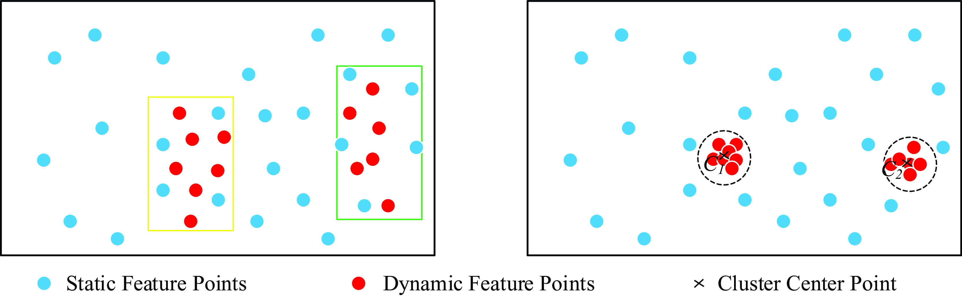
Firstly, after extracting the dynamic feature points from the dynamic mask, the k-means clustering algorithm is used to cluster these points, and the corresponding number of clusters is performed according to the number of moving objects in the image. The center point of each cluster is represented as $C_{i}$ , as shown in Figure 11.

Figure 11.

The k-means clustering algorithm is used to analyze the dynamic feature points in the image frame. According to the number of dynamic objects, the corresponding clustering operation is performed. Finally, each cluster will have a center point as a representative.

Next, the Euclidean distance $S_{i}$ from each static feature point to each cluster center $C_{i}$ is calculated. Then, the average distance $S$ from the static feature points to all cluster centers is calculated. Finally, according to the preset segmentation threshold, the weight value $Q_{i}$ of each feature point is determined, as shown in Figure 12.

Figure 12.

The weight distribution of static feature points is shown. The weight of each static feature point is calculated according to its average distance to the clustering center of each dynamic object, and then these weights are integrated into the pose optimization thread.

The static feature points close to the dynamic points have low output values and relatively small contribution to pose optimization, which helps to reduce the fluctuations caused by dynamic objects. In contrast, static feature points away from dynamic points have higher output values and are more important for pose optimization. These points are more stable and reliable.

For optimization, the reprojection error function is multiplied by the weight values of the feature points; feature points with larger weights are more reliable and contribute more to the objective function, and feature points with smaller weights contribute less. The optimization variable has been changed from the original camera pose to camera pose and the weights of feature points. The optimized feature point weight can more accurately characterize the reliability of the point, and its objective function is updated according to the weighted projection error:

(7) \begin{equation} \left\{R^{*},t^{*},Q^{*}\right\}=\underset{R,t,w_{i}}{\rm argmin}\frac{1}{2}Q_{i}\sum _{i=1}^{n}\| x_{i}-\pi \left(RX_{i}+t\right)\| _{2}^{2}\end{equation}

where $Q_{i}$ is the weight of map point $x_{i}$ .

In pose estimation, the optimization is performed jointly for the rotation matrix $R$ , translation vector $t$ , and the weights $Q_{i}$ of the map points $X_{i}$ . The Levenberg–Marquardt algorithm in the g2o library is used to deal with the joint optimization task. At the same time, it is necessary to manually calculate the partial derivative of the error term to the optimization variable, so the partial derivative of the feature point weight is:

(8) \begin{equation} \frac{\partial e}{\partial Q_{i}}=\left[\begin{array}{l} u_{i}-\left(\dfrac{X}{Z}\,f_{x}+c_{x}\right)\\[8pt] v_{i}-\left(\dfrac{Y}{Z}\,f_{y}+c_{y}\right)\\[8pt] u_{i}-\left(\dfrac{X}{Z}\,f_{x}+c_{x}-\dfrac{b_{f}}{Z}\right) \end{array}\right]\end{equation}

where $f_{x} , f_{y} , c_{x} , c_{y}$ and $b_{f}$ are camera parameters, $P=(\begin{array}{lll} X & Y & Z \end{array})^{T}$ is the spatial point coordinates in the camera coordinate system, and $(u_{i},v_{i})$ is the corresponding pixel coordinate point.

3.4. NeRF dense map

NeRF reconstructs 3D scenes by training a series of 2D images from different viewpoints. The continuous scene can be expressed as a function $F_{{\Theta} }\colon (\mathbf{x},\mathbf{d})\rightarrow (\mathbf{c},\sigma )$ , where $\mathbf{x}$ is the 3D coordinate position of a spatial point, and $\mathbf{d}=(dx,dy,dz)$ is the 3D Cartesian unit vector representing the direction $(\theta ,\phi )$ . $\mathbf{c}=(r,g,b)$ is the 3D point color of the point related to the perspective, and $\sigma$ is the density corresponding to the 3D position.

By using a multi-layer perceptron (MLP) network model to approximate the mapping relationship between input and output, an ‘implicit representation’ of the 3D scene is created. According to the above definition, for any light $\mathbf{r}(t)=\mathbf{o}+t\mathbf{d}$ , its light color $C(r)$ in the near boundary and far boundary interval $[t_{n},t_{f}]$ can be expressed by integral:

(9) \begin{equation} C\left(r\right)=\int _{t_{n}}^{t_{f}}T\left(t\right)\cdot \sigma \left(\mathbf{r}\left(t\right)\right)\cdot \mathbf{c}\left(\mathbf{r}\left(t\right),\mathbf{d}\right)dt\end{equation}

where $T(t)$ is the cumulative transparency of the light from $t_{n}$ to $t$ :

(10) \begin{equation} T\left(t\right)=\exp\left(-\int _{t_{n}}^{t}\sigma \left(\mathbf{r}\left(s\right)\right)ds\right)\end{equation}

In the NeRF rendering step, the color and voxel density of the three-dimensional points obtained during the reconstruction process are used to integrate along the ray and obtain the final two-dimensional image pixel value.

In practice, it is challenging for NeRF to accurately estimate continuous 3D information, and the corresponding implementation code cannot perform continuous integration. Therefore, it is necessary to discretize on the basis of Eq. (12). N points are sampled uniformly in the area where the quadrature is needed for approximate calculation. The $i$ -th sampling point can be expressed as:

(11) \begin{equation} t_{i}=\mathbf{U}\left[t_{n}+\frac{i-1}{N}\left(t_{f}-t_{n}\right),t_{n}+\frac{i}{N}\left(t_{f}-t_{n}\right)\right]\end{equation}

based on these sampling points, $C(r)$ can be simplified as follows:

(12) \begin{equation} \hat{C}\left(\mathbf{r}\right)=\sum _{i=1}^{N}T_{i}\cdot \left(1-\exp\left(-\sigma _{i}\cdot \delta _{i}\right)\right)\cdot \mathbf{c}_{i}\end{equation}

where $\delta _{i}=t_{i+1}-t_{i}$ is the distance between two adjacent sampling points. Therefore, $T(t)$ can be expressed as follows:

(13) \begin{equation} T_{i}=\exp\left(-\sum _{j=1}^{i-1}\sigma _{j}\delta _{j}\right)\end{equation}

Based on this rendering method, the NeRF function can be used to render the image from any angle. After processing the dynamic environment, NeRF rendering is performed on the image frame. Firstly, the position needs to be passed to NeRF as input. By minimizing the reprojection error, BA is used for pose optimization. After inputting the camera position and key frame into NeRF, the photometric error is minimized by the regression of the image color. The ray can be determined by giving the key frame $(K,[R|t])$ and the pixel coordinate $(u,v)$ :

(14) \begin{equation} r\left(d\right)=\left(-R^{T}t+dR^{T}K^{-1}\left[u,v,1\right]^{T}\right),d\in \mathrm{\mathbb{R}}\end{equation}

Optical sampling is performed near the surface of the ray, but only selective sampling is performed in the static region. Finally, the NeRF luminosity loss function $L$ is expressed as the L2 norm between the predicted color $\hat{C}(\mathbf{r}_{ij})$ and the pixel color $C(\mathbf{r})$ :

(15) \begin{equation} L=\sum _{ij}\left\| C\left(\mathbf{r}_{ij}\right)-\hat{C}\left(\mathbf{r}_{ij}\right)\right\| _{2}\end{equation}

When performing NeRF rendering, the mask obtained by segmenting the dynamic region is used to determine whether to render, and the image is generated by light sampling for each point in the scene to calculate the radiance of the light passing through the point. Because the dynamic part is beyond the sampling range, the dynamic part will appear as artifacts in the rendering process. When the dynamic object leaves the scene, the background occluded by the dynamic object in the previous rendering is repaired in the subsequent rendering to achieve the effect of background repair.

4.1. TUM dataset

The TUM RGB-D dataset contains many image sequences captured by RGB-D cameras in dynamic environments, as well as accurate ground-truth trajectories and camera internal parameters. Since the main purpose of dynamic SLAM is to improve the SLAM system in dynamic scenes, four groups of f3 sequences in high- and low-dynamic sequences were selected for each, f3-w/half, f3-w/rpy, f3-w/static, f3-w/xyz, f3-s/half, f3-s/rpy, f3-s/static, and f3-s/xyz totaling eight groups (the first four groups are high dynamic and the last four groups are low dynamic). Among them, w and s represent walking and sitting posture sequences, respectively, and half, rpy, static and xyz represent different motion modes of the camera, respectively.

4.2. Bonn dataset

The Bonn dataset uses the ASUS Xtion Pro LIVE camera to capture RGB-D images, including 24 dynamic sequences, such as crowd walking, balloon throwing, and moving boxes. Each scene can access the ground live camera trajectory. A comprehensive evaluation experiment was conducted on the performance of the algorithm proposed in this paper. Seven sequences were selected from the Bonn dataset for experiments, excluding sequences without static points in the entire view.

Among the selected sequences, the ‘balloon’ sequence captures the moment a person throws a balloon, while constantly hitting the balloon to prevent it from falling, while the ‘crowd’ sequence depicts a scene in which five people walk randomly in a room. The ‘person-tracking’ sequence captures the scene where the camera tracks the walking person. These complex scenarios further evaluate the performance of the RNF-SLAM system under various conditions.

4.3. Self-collected dataset

To address the limitations of publicly available datasets, this study constructed a real-scenario data acquisition platform, as shown in Figure 13. The platform was built based on the NOKOV optical system, featuring a multi-view infrared camera array that achieves submillimeter-level accuracy in spatial positioning and full coverage of dynamic areas. Three-dimensional reconstruction was performed using reflective markers to obtain six-degree-of-freedom pose ground truth. Multiple experimental groups were designed: the Static group for static scene acquisition (static); the Single-Person Motion group containing linear, rotational, and compound movements (one_move); the Dynamic Load group to test algorithm stability under non-rigid loading conditions (move_box); and the Multi-Person Interaction groups to verify the algorithm’s parsing capability in complex environments(two_move/three_move). These experiments provide reliable support for validating the robustness of the RFN-SLAM algorithm in dynamic environments.

Figure 13.

Dataset acquisition platform. The D435i camera moves within the effective area, captures poses through the Mars1.3H lens, and outputs true motion trajectory values.

4.4. Evaluating indicator

In the experiment, this paper uses ATE and RPE to measure the experimental results, and RMSE can be used for statistics. It is assumed that the estimated pose is expressed as: $P_{1},\ldots ,P_{n}\in SE(3)$ , and the real pose is expressed as: $Q_{1},\ldots ,Q_{n}\in SE(3)$ . ATE directly calculates the difference between the true value of the camera pose and the estimated value of the SLAM system, which can intuitively reflect the accuracy of the algorithm and the global consistency of the trajectory. The ATE of frame $i$ is defined as follows:

(16) \begin{equation} F_{i}\,:\!=\,Q_{i}^{-1}SP_{i}\end{equation}

where $S$ is the similarity transformation matrix from the estimated pose to the real pose, and RMSE can be used to count ATE:

(17) \begin{equation} \mathrm{ATE}_{\text{RMSE}}=\sqrt{\frac{1}{n}\sum _{i=1}^{n}||F_{i}||^{2}}\end{equation}

RPE mainly describes the accuracy of the two-frame pose difference between the fixed time difference, which is equivalent to the error of the direct measurement odometer. Therefore, the RPE of frame $i$ is defined as follows:

(18) \begin{equation} E_{i\vdots }=\left(Q_{i}^{-1}Q_{i+{\unicode[Arial]{x0394}} }\right)^{-1}\left(P_{i}^{-1}P_{i+{\unicode[Arial]{x0394}} }\right)\end{equation}

where $\bigtriangleup$ is the interval time, RMSE is used to calculate RPE:

(19) \begin{equation} \mathrm{RPE}_{\text{RMSE}}=\sqrt{\frac{1}{n}\sum _{i=1}^{n}||E_{i}||^{2}}\end{equation}

The improvement of ORB-SLAM3 algorithm in this paper is expressed as:

(20) \begin{equation} \textit{Improvement}=\frac{\mu -r}{\mu }\times 100\%\end{equation}

where $\mu$ represents RMSE or S.D of ORB-SLAM3; $r$ represents RMSE or S.D of RFN-SLAM.

4.5. Compared with other advanced SLAM system experimental results

The RNF-SLAM system is compared with four advanced dynamic SLAM systems, including the original ORB-SLAM3, OVD-SLAM [Reference He, Li, Wang and Wang32], LC-SLAM [Reference Du, Huang, Mu, Zhao, Martin and Xu33], MR-SLAM [Reference Zhang and Li34] and the proposed algorithm RFN-SLAM method. In each group of experiments, the RMSE and S.D of the ATE of each system are given to measure its global robustness and stability, and the RMSE and S.D of the RPE are used to measure the local performance.

4.5.1. Analysis of experimental results of TUM dataset

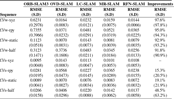
A comprehensive ATE quantitative comparison was performed on the experimental sequences selected in the TUM dataset, and the comparison indicators were RMSE and S.D. The proposed method achieves the best performance in most sequences, as shown in Table II. RFN-SLAM is usually superior to other methods in terms of RMSE of most sequences. For example, in the ‘f3/w-xyz’ sequence, there are two people walking back and forth as moving objects, and they occupy a large area in the current frame. At this moment, RFN-SLAM effectively determines the moving objects, but ORB-SLAM3 does not distinguish them. As a result, the RMSE of RFN-SLAM is the lowest (0.0144), while the RMSE of ORB-SLAM3 is the highest (0.6231). Compared with ORB-SLAM3, RMSE is significantly increased by 97.6%, and S.D is significantly increased by 97.8 %. In the sequences of ‘fr3/w-rpy’, ‘fr3/w-xyz’ and ‘fr3/w-static’, RFN-SLAM continues to show low RMSE, highlighting its excellent accuracy. When evaluating the S.D of the error, RFN-SLAM performs well, and usually the S.D value is the lowest or close to the lowest. For example, in the ‘fr3/w-xyz’ sequence, the SD of RFN-SLAM is 0.0066, which is significantly lower than that of ORB-SLAM3 (0.2978), which shows the high stability of its performance. In contrast, ORB-SLAM3 showed competitive RMSE in ‘fr3/s-xyz’. In this sequence, the motion trend of the moving objects is not obvious, or even nearly stationary. The weighting approach adopted by RFN-SLAM appears to be over-corrected, resulting in inferior performance to ORB-SLAM3. However, in ‘fr3/w-rpy’, ORB-SLAM3 has the highest RMSE. This indicates that its performance fluctuates greatly in different scenarios. The performance of OVD-SLAM, LC-SLAM and MR-SLAM is relatively balanced. RMSE and S.D are neither the lowest nor the highest, which means that they are consistent in accuracy, but not necessarily optimal. In general, these data strongly support the conclusion that the proposed RFN-SLAM method exhibits better accuracy and stability in the test sequence.

Table II.

Results of metric ATE on TUM RGB-D dataset.

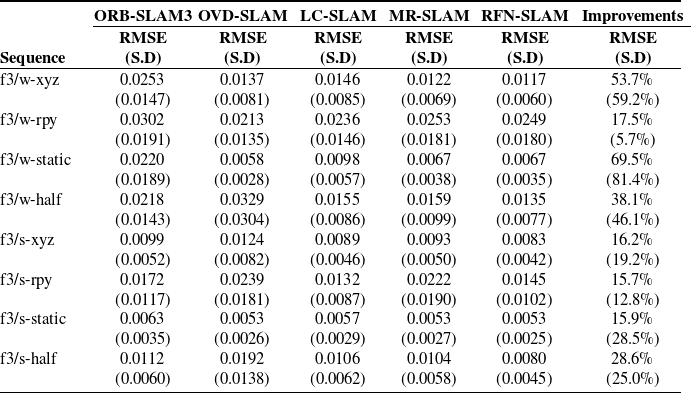
Table III quantitatively analyzes the RPE of various SLAM methods and evaluates the accuracy and stability through RMSE and S.D. Comparing RMSE, the performance differences between different sequences and methods were observed. RFN-SLAM shows competitive or lower RMSE in most cases, indicating its robustness and effectiveness. The S.D value further illustrates the consistency of each method. For example, in ‘fr3/w-static’, the S.D of RFN-SLAM is 0.0035, showing its consistency. In contrast, ORB-SLAM3 has a higher S.D value (0.0189) in ‘fr3/w-static’, indicating that its performance is more variable. Compared with ORB-SLAM3, the S.D of RFN-SLAM in this sequence was significantly increased by 81.4%. Overall, the experimental data quantitatively confirm the advantages and disadvantages of each SLAM method in different environments. However, the RFN-SLAM method shows significant advantages, and it can balance accuracy and consistency in most cases.

Table III.

Results of metric RPE on TUM RGB-D dataset.

Figure 14 shows the error between the estimated trajectory of the ORB-SLAM3 and RFN-SLAM algorithms and the actual trajectory on the ground. Through observation, the original ORB-SLAM3 has obvious errors in the high-dynamic sequence, which is inconsistent with the actual ground conditions. In contrast, the RFN-SLAM algorithm can calculate the estimated trajectory that closely matches the original trajectory, and achieve more accurate positioning in a dynamic environment. Figure 15 shows the operation in the sequence ‘fr3/w-static’. By comparing ORB-SLAM3, RFN-SLAM shows significant advantages, which can effectively eliminate the feature points related to dynamic objects, so as to ensure the stable operation of the system.

Figure 14.

In the high-dynamic scene of the TUM RGB-D dataset, the ATE of ORB-SLAM3 and RFN-SLAM is compared. The black line represents the real trajectory of the camera motion, the blue line represents the estimated trajectory, and the red line represents the difference between the estimated trajectory and the real trajectory.

Figure 15.

The feature point extraction results of ORB-SLAM3 and RFN-SLAM in ‘fr3/w-static’ sequence are compared. RFN-SLAM can effectively detect and eliminate the feature points of dynamic objects.

NeRF rendering is performed on the sequence of the selected experiment on the TUM dataset, such as the effect of rendering the ‘fr3/w-xyz’ sequence, as shown in Figure 16. Because the proposed algorithm RFN-SLAM is only adopted in the static area, when the dynamic object enters the scene, it will not be adopted. When it is separated from the scene, NeRF will correct the lost part of the previous rendering (i.e., the background occluded by the dynamic object), so as to achieve the effect of background repair, and the map of the static scene will be obtained. RFN-SLAM reduces the influence of dynamic objects on the system at the front end, makes the camera pose estimation more accurate, and provides a more accurate camera position for NeRF rendering to achieve better rendering results in a dynamic environment.

Figure 16.

The results of 3D reconstruction of the ‘fr3/w-xyz’ sequence of the TUM dataset using RFN-SLAM only reconstruct the static part. (a) input; (b), (c) and (d) reconstruction.

4.5.2. Analysis of experimental results of Bonn dataset

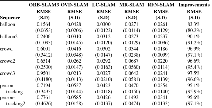
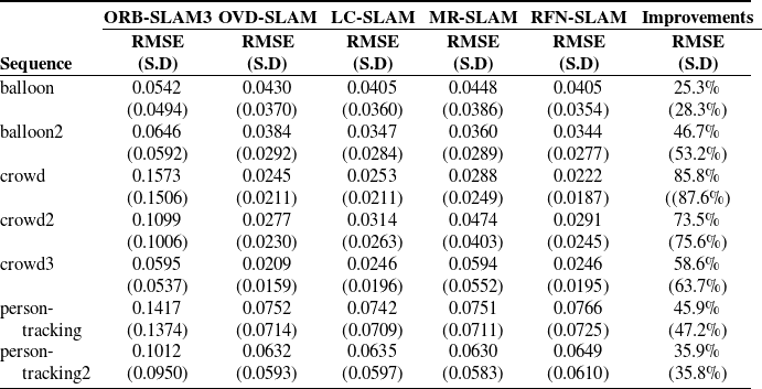
The selected sequences were compared in the Bonn dataset, and a comprehensive ATE quantitative comparison was performed, as shown in Table IV. In crowded scenes (such as ‘crowd’, ‘crowd2’ and ‘crowd3’), the motion estimation deviation of ORB-SLAM3 is obvious and deviates from the actual trajectory. In the ‘crowd’ sequence, personnel movement is large and densely distributed, resulting in fewer static feature points to be extracted. RFN-SLAM is able to show better performance advantages by removing dynamic feature points and using static weighting. RFN-SLAM has the lowest RMSE (0.0186), while ORB-SLAM3 has the highest RMSE (0.6001). Compared with ORB-SLAM3, the RMSE of RFN-SLAM is increased by 96.9 %. In other sequences, RFN-SLAM continues to show low RMSE, highlighting its excellent accuracy. RFN-SLAM also performs well when evaluating the S.D of the error. For example, in the ‘person-tracking2’ sequence, the SD of RFN-SLAM is 0.0133, which is significantly lower than that of ORB-SLAM3 (0.4626), fully demonstrating the high stability of its performance. During the experiment, it is found that other advanced algorithms sometimes lose cameras in these sequences. The reason is that dense crowds are the key characteristics of the scene, and the movement of people may occupy a large range. After the removal of dynamic feature points, the remaining static feature points are not enough to support accurate camera pose matching and estimation, and the RFN-SLAM system proposed in this paper can better handle similar situations. Through experiments, it is fully proven that the RFN-SLAM method has significant advantages in accuracy, stability and robustness in complex scenes containing many dynamic objects.

Table IV.

Results of metric ATE on Bonn dataset.

Table V quantitatively analyzes the RPE of various SLAM methods on the Bonn dataset. Through chart data analysis, RFN-SLAM shows lower RMSE in most experimental scenarios. For example, in the sequence ‘crowd’, the RMSE (0.0222) of RFN-SLAM can obtain better advantages than other SLAM algorithms, indicating its robustness and effectiveness. At the same time, in ‘crowd’, the S.D of RFN-SLAM is 0.0187, showing its consistency.

Table V.

Results of metric RPE on Bonn dataset.

Figure 17 clearly shows the gap between the estimated trajectory and the real trajectory of ORB-SLAM3 and RFN-SLAM algorithms in dynamic scenes. The estimation deviation of ORB-SLAM3 is obvious, which is mainly limited by the influence of dynamic objects. In contrast, the RFN-SLAM algorithm can effectively deal with dynamic objects, thus providing more accurate positioning and higher accuracy. Figure 18 shows the actual operation in the sequence crowd2. By comparing ORB-SLAM3, RFN-SLAM shows significant advantages, which can effectively eliminate the feature points related to dynamic objects, so as to ensure the stable operation of the system.

Figure 17.

Comparison of the ATE of ORB-SLAM3 and RFN-SLAM in some dynamic scenes of the Bonn dataset. The black line represents the real trajectory of the camera motion, the blue line represents the estimated trajectory, and the red line represents the difference between the estimated trajectory and the real trajectory.

Figure 18.

The feature point extraction results of ORB-SLAM3 and RFN-SLAM in the ‘crowd2’ sequence are compared. RFN-SLAM can effectively detect and eliminate the feature points of dynamic objects.

Figure 19 shows the dense reconstruction of RFN-SLAM algorithm under dense human activities (such as ‘crowd2’ sequence). The figure shows that the crowd is effectively excluded and focuses on the reconstruction of static scenes. By removing dynamic objects, the accuracy of pose estimation is improved, which significantly improves the quality of reconstructions with tables, figures may be presented at appropriate locations within the text. Figure captions should be below the figure itself, as shown below.

Figure 19.

The results of 3D reconstruction of the ‘crowd2’ sequence of the Bonn dataset using RFN-SLAM only reconstruct the static part. (a) input; (b) and (c) reconstruction.

4.5.3. Analysis of experimental results of self-collected dataset

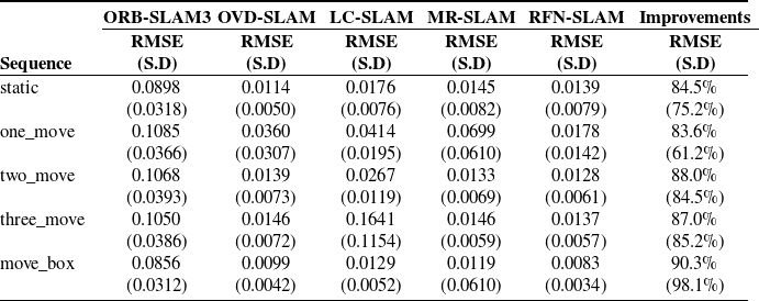
The data in Table VI reveals that RFN-SLAM demonstrates all-round performance enhancement in static environments, dynamic scenarios and load handling scenarios. In the static sequence, RFN-SLAM achieves RMSE = 0.0139, which is 84.5% improvement over ORB-SLAM3, and its S.D. reduction reaches 75.2%, which verifies the optimization effect of the base positioning accuracy. As the number of dynamic interference sources increases (two_move to three_move), RFN-SLAM maintains RMSE<0.0137 (S.D.<0.0061), which maintains more than 87.0% error reduction over the baseline algorithm. Particularly in the sequence move_box, RFN-SLAM achieves an RMSE of 0.0083 (IMP 90.3%) with an S.D. of 0.0034, which is 94.4% lower than MR-SLAM. Although OVD-SLAM has a slightly better RMSE in some scenarios (e.g., static), RFN-SLAM maintains the lead in terms of overall dynamic performance.

Table VI.

Results of metric APE on self-collected dataset.

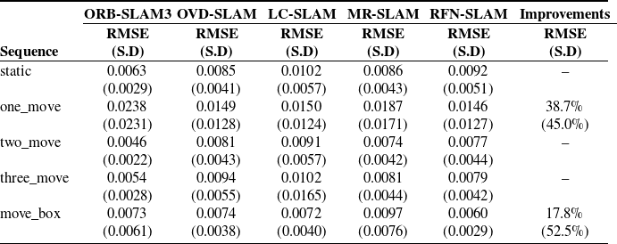
The RPE data in Table VII further reveals the algorithm characteristics. In the sequence one_move, RFN-SLAM has an RMSE of 0.0146, which is a 38.7% improvement and a 45.0% reduction in S.D. compared to ORB-SLAM3 (0.0238), reflecting its ability to suppress localized motion disturbances. In the sequence move_box, its RMSE is further optimized to 0.0060 (IMP 17.8%) and the S.D. is only 0.0029, which is 52.5% lower than that of ORB-SLAM3 (0.0061). Although its RMSE has a slight disadvantage of 4.3% to 7.8% in the sequences two_move and three_move, its control of error fluctuation is more robust. In addition, RFN-SLAM has an RMSE of 0.0092 in sequence static, which is slightly inferior to ORB-SLAM3 (0.0063), but its S.D. value (0.0051) is close to that of OVD-SLAM (0.0041), and it is still better than LC-SLAM (0.0057). This result shows that RFN-SLAM significantly improves the localization robustness in dynamic environments while ensuring the basic performance in static scenes.

Table VII.

Results of metric RPE on self-collected dataset.

Figure 20 shows the trajectory comparison between ORB-SLAM3 and RFN-SLAM on the self-picked dataset. Through the comparison, the obvious advantages of RFN-SLAM in terms of trajectory accuracy and stability can be visualized. Especially in the dynamic and complex scenario of sequence move_box, RFN-SLAM effectively suppresses the accumulation of errors caused by environmental changes. The dynamic feature point processing mechanism of RFN-SLAM successfully avoids the expansion of errors, showing its excellent dynamic adaptability and robustness. Compared with the ORB-SLAM algorithm, RFN-SLAM is able to maintain high trajectory accuracy when facing complex dynamic scenes, which proves its strong stability and reliability in dynamic environments. This performance validates the superiority of RFN-SLAM in dealing with complex environmental changes, especially its potential to improve system performance and accuracy.

Figure 20.

Comparison of the ATE of ORB-SLAM3 and RFN-SLAM in all dynamic scenes of the self-collected dataset. The black line represents the real trajectory of the camera motion, the blue line represents the estimated trajectory, and the red line represents the difference between the estimated trajectory and the real trajectory.

Figure 21 presents the distribution characteristics of dynamic object feature points between ORB-SLAM3 and RFN-SLAM in the real scene sequence ‘one_move’. The experimental results show that RFN-SLAM accurately filters out the feature points on the surface of a dynamic object in a multi-frame sequential image sequence through the dynamic feature discrimination mechanism, thus providing stable and reliable feature information to support the camera pose estimation. In contrast, ORB-SLAM3 lacks the ability to discriminate between dynamic and static features, and its feature point set contains a large amount of dynamic object information. This comparative experimental result further validates the superiority of RFN-SLAM in dynamic scenarios. Figure 22 shows the reconstruction results of RFN-SLAM for the ‘move_box’ sequence without dynamic object dense map. As can be seen from the figure, the algorithm not only successfully removes the moving objects in the scene, but also performs a complete geometric reconstruction of the background region that is occluded by them.

Figure 21.

The feature point extraction results of ORB-SLAM3 and RFN-SLAM in the ‘one_move’ sequence are compared. RFN-SLAM can effectively detect and eliminate the feature points of dynamic objects.

Figure 22.

The results of 3D reconstruction of the ‘move_box’ sequence of the self-collected dataset using RFN-SLAM only reconstruct the static part. (a) input; (b) and (c) reconstruction.

4.5.4. Time performance analysis

In practical engineering applications, the real-time performance of an algorithm is a key indicator of its applicability. In this study, the temporal performance of RFN-SLAM is verified by comparing its computational efficiency with that of existing dynamic visual SLAM algorithms on TUM and Bonn standard datasets. As shown in Table VIII, the average processing time of the RFN-SLAM system for a single-frame image is 84.2 ± 1.5 ms, which is able to meet the requirements of mobile robot platforms. Compared with the benchmark algorithm ORB-SLAM3, RFN-SLAM keeps the computational elapsed time within 2.8 times of that of ORB-SLAM3 while maintaining a higher localization accuracy, demonstrating the Pareto-optimized characteristics of accuracy and efficiency.

Table VIII.

Real-time comparison of VSLAM algorithms in dynamic environments.

Table IX presents the average computational time distribution of the RFN-SLAM algorithm for each functional module, covering the RT-DETR thread, the FAST-SAM thread, and the Tracking thread as the main thread. Among them, the Tracking thread, as the core control module of the system, takes significantly longer than the two sub-threads, which is determined by the complexity of the main tasks such as global pose estimation and map maintenance. In the FAST-SAM thread, the computational overhead of this module is relatively high due to the two-phase segmentation process involved; while the RT-DETR thread significantly reduces the computational time consumption through algorithm optimization, and demonstrates efficient target detection capability. From the perspective of overall system performance, the comprehensive computation time of RFN-SLAM can meet the real-time requirements of most real-world scenarios, which indicates that the algorithm has good potential for engineering applications while guaranteeing the functional integrity of the algorithm.

Table IX.

Comparison of time consumption of each module of RFN-SLAM algorithm.