


1. Introduction
I have been conducting research into electroacoustic music since the end of the 1990s. My first studies focused on terminology and then, from the beginning of the 2000s, on the analysis of electroacoustic fixed works or acousmatics. I developed a protocol for the creation of graphic representations resulting from these analyses (Couprie Reference Couprie, Bhagwati and Bresson2018) that can be used to communicate the content of a musical analysis, to help the teacher and the student in a learning situation, to introduce contemporary creation to a neophyte audience or simply to enhance awareness in young children. Visuals then became an important part of my research. They are both indispensable listening aids for music that often has no score or when scores are very incomplete, such as in the case of mixed music, and facilitate the transmission of explicit or implicit elements of analysis that are sometimes highly complex. After making numerous transcriptions and experimenting with widely differing techniques and methods, I continued my research work into the subject of morphology and its place in the construction of structures at all levels, from the microstructures present in musical objects to the form. At the time, major analysis techniques were based on segmentation into units – sound objects (Schaeffer Reference Schaeffer1966), sound-images (Bayle Reference Bayle1993), spectromorphologies (Smalley Reference Smalley1997), functions (Roy Reference Roy2003), temporal semiotic units (Rix and Formosa Reference Rix and Formosa2008), time-fields (Thoresen and Hedman Reference Thoresen and Hedman2015) among others – and the use of classification methods by similarity, by origin in the creative process – as in paradigmatic or generative analysis – or by function in the construction of form. One of the dominant characteristics in electroacoustic creation since the 1970s is the use of sound materials that resist musical analysis because of their duration, the imprecision of their temporal and spectral borders, their continuous evolution or the virtuosity of their constitutive morphologies. In the same way, the object-structure couple proposed by Schaeffer (Schaeffer Reference Schaeffer1966: 375–6) makes it difficult to analyse structures that are often heterarchical and elusive, even if the link between form and morphology remains evident.
I then turned to acoustic analysis and data representation to analyse morphologies, not in the form of well-identified units but rather in the form of evolution, singularities, focal points, zones, in short moments that are difficult to isolate but are still clearly perceptible. I therefore developed a framework bringing together my transcription techniques with these new methods based on representations made from descriptors extracted from the audio signal, which is briefly presented in Section 3. In Section 2, I introduce the context for the development of the framework within the scope of interdisciplinary musicology and research-creation. Finally, Section 4 describes three analytical approaches applied to electroacoustic improvisation based on recordings made with the Paris-based group Les Phonogénistes.Footnote 1
2. Analysing Electroacoustic Music
2.1. Interdisciplinarity methods and research-creation
Since the 1990s, research in musicology has gradually opened up to other methodological fields. Jean-Jacques Nattiez notes that musical phenomena can no longer be studied through a single approach; he advocates a ‘general musicology’ that is open and limitless in its investigations (Nattiez Reference Nattiez2007: 1205–6). Critical musicology and postmodern musicology (Scott Reference Scott and Sim1998: 114–115) integrate other human sciences. It is clear that researchers can no longer avoid new questions that often require expertise going far beyond their own field of competence. I have already demonstrated how this openness to interdisciplinarity seems to have become an essential approach in musicology (Couprie Reference Couprie2020). Regarding the integration in musicology of some methods derived from the exact sciences, as early as 2005, Nicholas Cook noted the importance of the use of methods for studying the audio signal and extracting information for musicology with music information retrieval (MIR) methods. Much earlier, in 1960,Footnote 2 Pierre Schaeffer was one of the first to promote interdisciplinary work in the field of musical research and Jean-Claude Risset, a pioneer in this field (Risset Reference Risset2010) having a dual scientific and musical background, throughout his life combined his musical creations with his scientific research.
Research-creation is part of this interdisciplinary momentum, combining as it does musicology, musical aesthetics, philosophy, computer science and musical acoustics among others. It brings together a set of methods that consist in retracing the act of creation as with musical genetics, or broadly speaking, the creative process itself. Whereas these simply retrace the history of creation or deconstruct the various orientations of the complex process that is the source of the creative act – historical, philological, analytical or sociological – research-creation evolves within a fruitful dialogue between research and creation in the broadest sense of the term. Although it is often wrongly associated with a vague intention to render the creative act scientific (Stévance and Lacasse Reference Stévance and Lacasse2013: 17), it is more a question of considering not just the work of the composer but also that of the performer, the computer music director and all those involved in a creation, interpretation, performance or improvisation with a view to sharing knowledge. In terms of disciplinary combinations, this research is found in a form of ‘focused interdisciplinarity’ (Charaudeau Reference Charaudeau2010). It combines the artistic aspect of creation, focusing on aesthetic experience and the sharing of know-how – the non-scientific part of musical research concerning non-formalised empirical knowledge – with the scientific aspect of musicology that allows possible refutability and reproducibility of experiences (Popper 1973: 38).
In fact, much research into electroacoustic music or contemporary creation in general is a matter of research-creation. Not only is this research model particularly suited to the work of researchers who are also often composers or musicians but also the practice and the study of electroacoustic music require a much wider range of skills than those of composers of instrumental music. The composer–performer–researcher in electroacoustic music must also develop their studio or performance devices and interfaces, use complex software, or even develop their own software, and face constraints far more demanding than those encountered in the practice of instrumental music or that of simple musicology.Footnote 3
2.2. Analysing electroacoustic music improvisation
Learning improvisation is a practical matter: there is no exclusively theoretical side to improvisation. (Bailey Reference Bailey1992: 8)
It is commonly accepted that electroacoustic music resists analysis. The challenges are threefold: the absence of visual support, the complexity of analysing sound material and structures, and the complexity of studying music that requires skills that go far beyond the strictly musical domain. I will now add a further challenge with the analysis of improvisation in the practice of electroacoustic music. Analysing or simply studying improvisation is often considered impossible because improvisation is not an object, a ‘thing’, a structure that can be broken down into its constituent parts, but rather an ephemeral moment, ‘a mode of action, or even an attitude, that involves not only degrees of spontaneity but also an implicit or explicit valuation of such freedom with respect to the activity’ (Sheehy 2013: 1). This ‘mode of action’ implies first, that it is very difficult to record an improvisation and then study it, and that second, it is not really relevant to study this practice with the traditional tools of musicology. We can also see in improvisation a beneficial action contributing to the practice of writing or musical interpretation. The concept of improvisation is not an alternative to composition (Dahlhaus 2010) nor is it in opposition to performance or interpretation (Cook Reference Cook2013: 226).
The case of electroacoustic improvisation is unique because, from the very beginning of musique concrète, the practice of improvisation has been integrated in the creation of sound material. Thus, Pierre Henry relates his entrance exam to Pierre Schaeffer’s studio with a prepared piano improvisation test (Henry Reference Henry2017: 21), a prelude to numerous recording sessions that will generate the sound material that is the source of their collaborative works. In addition, following the model of Pierre-Alexandre Tremblay, some composers use improvisation to create parts of their works later finalised in the studio (Tremblay Reference Tremblay2012). Since the 1990s, improvisation has become a relatively common practice in electroacoustics.Footnote 4 However, concerts are rarely advertised as being improvised and usually only regular listeners are aware that they are. Others may be surprised to find out after the concert that it was improvised. Some studies have even shown that there is no real difference between listening to a free improvised performance and a contemporary instrumental creation (Canonne Reference Canonne2019). There is no reason why this should not be the same in the case of electroacoustic improvisation.
The purpose of this article will not be to approach the study of electroacoustic improvisation from the perspective of the actual performance. I will focus on the object itself, that is, the musical result of the improvisation, or rather the trace left by the improvisation in the recording. The preparation that is often forgotten in musicological studies will also be taken into account here. This part is often very important since the actual performance can result from a long period of preparation with numerous rehearsals and the concerts that have preceded it. Although the experience in the closed studio or surrounded by an audience is very different, the presence of listeners does not guarantee the quality of the improvisation. Recordings performed in private or in public are therefore just as important for the musicologist. That is why in the last section of this article I will be addressing a wide selection of improvised fragments from rehearsals.
Having experienced the improvisations as a musician, my goal will be to analyse these recordings in an informed manner. I have known the musicians I have been playing with for many years as well as the software, devices and digital musical interfaces they use, the musical strategies they have developed and the way rehearsals are conducted. In this case, can these elements be identified through the analysis of audio recordings? In order to conduct the analysis, I will be using the framework presented in the next section.
3. A framework to analyse electroacoustic music
3.1. Complexity in electroacoustic music
In the field of electroacoustic music, composers and researchers have identified new formal models or new structures based both on expanded properties of sound (Couprie Reference Couprie, Emmerson and Landy2016a) and on an analysis of the material not as a chain of units but as a morphological continuity or flow. Thus, composers of spectral movement write about ‘flux’ as opposed to the composition of units (Murail Reference Murail and Michel2004: 14), Denis Smalley develops ‘spectromorphology’ (Smalley Reference Smalley1997) and François Bayle is strongly inspired by research into ‘morphogenesis’ (Bayle Reference Bayle1993: 85). The model that I will be describing has its roots in this research but is also strongly influenced by the exact sciences. It is therefore part of an interdisciplinary research project combining the humanities and exact sciences as discussed earlier. This model of analysis is based on the continuity of parameters as opposed to discretisation into units by using acoustic analysis and analytical representations (Couprie Reference Couprie2015). The aim is to consider both the macrostructures at the formal level involved in the development of musical discourse and the microstructures that are responsible for microvariations in the material or the articulations. The object-structure couple proposed by Schaeffer in 1966 (Schaeffer Reference Schaeffer1966: 375–6), which is often used as a reference for many analyses, does not provide a comprehensive overview as it does not multiply the levels of analysis and does not consider the structures in a fully hierarchical manner. Schaeffer considers the object as units that can be grouped together similar to the model of natural language (Schaeffer Reference Schaeffer1966: 294–314). This model, however, corresponds to the model of a scientifically structuralist-driven age, in which numerous studies have attempted to apply language structures to music.Footnote 5 From the 1960s on, many of the sound materials in electroacoustic works are characterised by lengthy textures, complex spectra, and slow and progressive developmentsFootnote 6 in which it is very difficult to isolate units that seem to be organised in structure and then in form. Electroacoustic music and improvisation are mostly composed of complex sounds that evolve over time and are difficult to isolate and analyse spectrally, that is, difficult to reduce without losing the complexity that makes them what they are. This complexity is characterised by a web of events (Morin Reference Morin2008: 5) that make up our perception. To freeze sound in one or more states in order to study it is to lose an important part of what constitutes the artistic intention of the composer or performer and which is precisely its temporal evolution. To describe these evolutions, the notion of morphogenesis, which has long gone beyond the field of biology, has provided me with some precious tools to research and describe the slow transitions of the spectrum so characteristic of François Bayle’s music (Couprie Reference Couprie and Bayle2016b). But the most important contribution has come from representations used in data analysis that allow us to visualise the complexity of the sound material hierarchically.
3.2. The framework
To facilitate the use of these representations as a complement to more usual analysis methods, I have developed a framework that describes both the techniques and the workflows used by the musicologist. I have created the EAnalysis software, then a version 5 of iAnalyse that allows all the steps of this workflow to be executed.
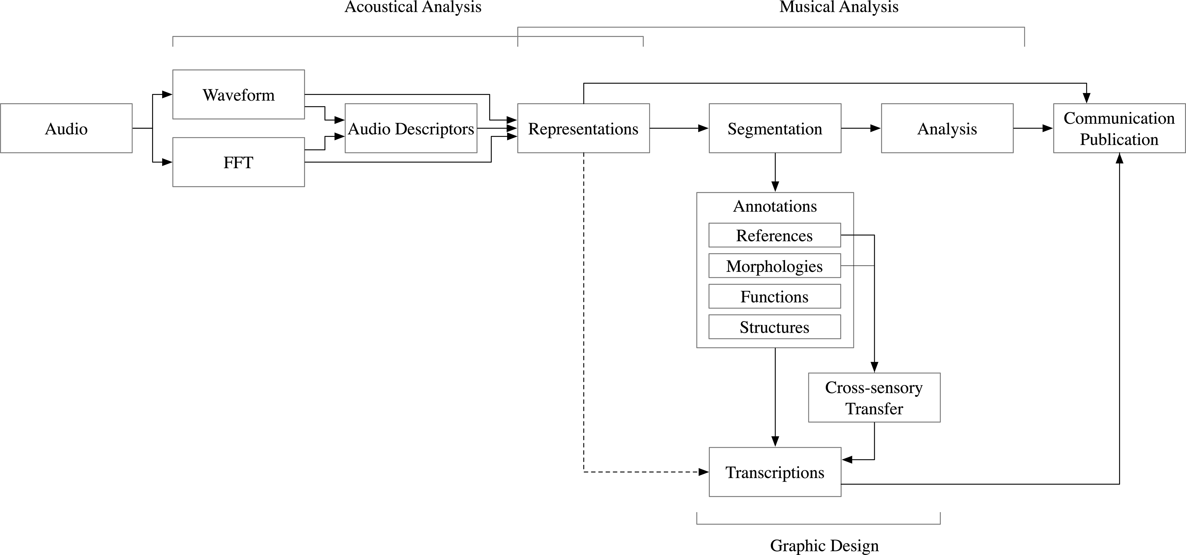
The framework (Figure 1) combines three areas of expertise: the acoustical analysis of digital audio files, the musical analysis itself based on the previous steps and the graphic design mixing data representation techniques, graphical modelling of the performance and techniques for transmitting the analysis. In this article I will focus on the first two areas. The third, mostly based on the annotation of representations designed to perform transcriptions, has already been described in detail in another article (Couprie Reference Couprie, Bhagwati and Bresson2018).
The framework for the analysis of electroacoustic music.

The method used with the framework always adheres to the following four steps:
-
1. The extraction of information from the digital audio file(s): this step is performed by the playback software – through the visualisation of a waveform or a fast Fourier transform (FFT) – or through the extraction of audio descriptors (MIR).
-
2. The computation of coefficients from the information extracted from the digital audio file: this optional step allows data to be obtained from statistical methods such as correlation,Footnote 7 standard deviationFootnote 8 and averages.Footnote 9
-
3. The visualisation of the previously extracted information: in the same way, this step is performed automatically by the audio playback software or manually with acoustic or data analysis technologies. Some visual displays are particularly efficient for musicology, as they permit easy linking of the values extracted from the signal to musical analysis parameters such as morphology, structure, timbre, intensity variations, tempo or time flow variations. This step is usually ignored and the representations used are those provided by the software with default settings. However, it is essential to develop customised representations that will avoid misinterpretation or missing relevant information.
-
4. The interpretation of results, analysis and creation of musical representations: this purely musicological step can be performed on the visual displays obtained during the previous step using annotations or may require the creation of ad hoc musical representations to facilitate analysis. The use of representation compilations makes it possible to interpret, formulate hypotheses or highlight correlations between various data extracted from the digital audio signal and parameters of the musical analysis.
These steps not only highlight the interaction between several very diverse fields of competence but also, and especially, a profound break in method in musicology, which seems to me to be an epistemological break (Couprie Reference Couprie2020). Audio is very difficult to study without a visual support, so we must use representations that although never perfect will still provide the basis for conducting the analysis. However, the playback of the digital audio file and its representations are simply interpretations, technological mediations, for which it is impossible to verify fidelity (Bachimont Reference Bachimont and Gayou2013: 26). The representations are generally not musical: the waveform is only a vague representation of sound intensity, the FFT is merely a vague estimation of the spectral content, and the descriptor of spectral centroid is simply a representation of sound brilliance that is particularly difficult to interpret musically. With the study of digital audio files, the musicologist therefore navigates through very approximate data for which one has to build the tools and methods to reveal their musical qualities.
3.3. Audio descriptors
Musicology has been using audio descriptors for some ten years, while they have been commonly used since the 1990s in the field of musical acoustics to identify and classify sounds according to their timbre, pitch, rhythm or pulse. A descriptor is a list of values representing one or more characteristics of the digital audio signal. It can be one-dimensional – such as the root mean square (RMS) amplitudeFootnote 10 or loudnessFootnote 11 – or multidimensional – such as the mel-frequency cepstral coefficients (MFCCsFootnote 12 ) or, more commonly, the FFT. Descriptors can be grouped into three categories (Serra et al. Reference Serra, Magas, Benetos, Chudy, Dixon and Flexer2013: 12):
-
1. Low-level descriptors computed on very short fragments of the signal and whose algorithms are robustFootnote 13 enough to produce reliable results (e.g., RMS amplitude or spectral centroid).
-
2. Medium-level descriptors that allow the extraction of information in pitch (fundamental frequency, inharmonicity) or time domain (pulse). The algorithms used are less robust than those of low-level descriptors, but their interpretation is easier for the musicologist.
-
3. High-level descriptors to characterise perceptual or semantic information (emotion, rhythm, tonality, harmony, musical genre). The algorithms used are also less robust and highly dependent on audio sources.
Descriptors have been developed for the analysis of harmonic and rhythmic popular music in which the spectrum is less dense and less complex than in electroacoustic music. The choice of relevant descriptors for the analysis of complex sounds used in electroacoustic music is therefore delicate. For the framework, I mainly use first-level and sometimes second-level descriptors such as inharmonicity measuring the level of complexity of the spectrum. These descriptors are classified in three categories:
-
1. Amplitude descriptors: RMS amplitude and sometimes loudness.
-
2. Descriptors to describe a spectrum quality: the spectral centroid or spectral rolloff,Footnote 14 the spectral variance.Footnote 15
-
3. Descriptors for classifying spectra: spectral flatnessFootnote 16 or zero crossing rateFootnote 17 (ZCR).
Most of these descriptors are difficult to interpret and, as noted previously, creating visual displays of these descriptors is not straightforward. It is thus necessary to choose relevant and efficient representations within a musicological framework without creating errors in their interpretation. The aim of these representations will be to guide the listener to parts that may go unnoticed, highlight implicit elements or facilitate navigation in long and complex audio files.
3.4. Audio feature representations
There are many types of data representation that can be used with audio descriptors, such as 2D or 3D graphs, histograms, areas, point clouds and radar. I have chosen to present two particularly efficient representations for musical analysis: the flow curve and the self-similarity matrix.
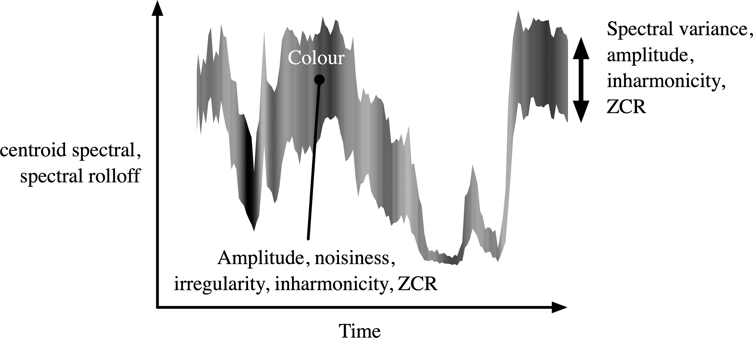
The brightness standard deviation (BStD), proposed by Mikhail Malt and Emmanuel Jourdan (Malt and Jourdan Reference Malt, Jourdan, Hascher, Ayari and Bardez2015), is based on a flux graph in which three descriptors are associated to constitute a single curve and to highlight the evolution of specific sound qualities that are used to qualify the timbre or the spectral colour. Figure 2 shows some examples of the distribution of the descriptors on the graph.
The principle of producing a BStD. Compared with other types of graphs, a flow curve such as BStD facilitates the interpretation and correlation between several descriptor data.

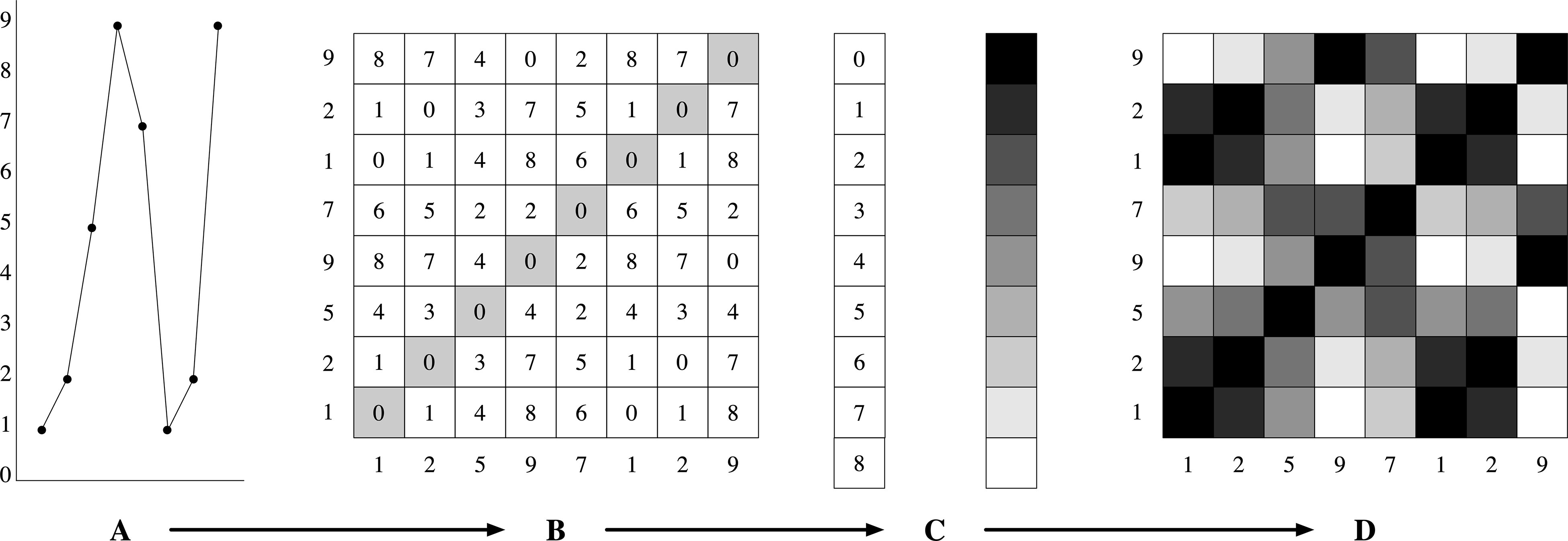
The self-similarity matrix highlights the structures underlying the data. It does not represent the values, but their similarities, that is, the distance between them. The computation is performed in two or three steps (Figure 3). The first step consists in computing the distances between each value of a graph (A) and putting them in a matrix (B). The diagonal (in grey in B) is the distance 0 representing the distance 0 that exists between the values and themselves.Footnote 18 The resulting matrix contains a very large number of values that are impossible to interpret, so the second step is to convert the values into colours (C), usually greyscale. This results in a coloured matrix (D) in which it is easy to identify groupings around points, areas or lines. A fourth step may be to colour this matrix in pseudo-colours, as used in medical imaging, to overcome the perception problems associated with the use of greyscale (Ware Reference Ware2000: 129).Footnote 19
The computation method of self-similarity matrix.

As I will demonstrate in the next part, the self-similarity matrix is very efficient for form analysis or for connecting microstructures and macrostructures. However, it is not easy to interpret. For convenience, matrices will always be interpreted horizontally. Five types of elements are clearly identifiable:
-
Lines drawn down the entire height indicate breaks or articulations.
-
Full-height bands that have the same alternating colours: these represent identical or close repetitions.
-
Wide areas with the same colour indicate stable values.
-
Areas that present horizontal gradients indicate gradual transitions.
-
Blocks that repeat around the diagonal suggest rhythmic patterns.
4. Analytical approaches
The preceding framework, the acoustic tools and the representations will allow me to show their efficiency for the analysis of electroacoustic improvisation examples. As I pointed out before, the framework only presents a guide for listening and analysis. All observations made on the representations require validation through listening. When validation is not possible by listening, it means that part of the graph does not correspond to a perceptible acoustic property or that the listening has not been perceptive enough. In the first case, either the acoustic property is irrelevant and will therefore be ignored, or it may indicate a specific configuration or technical defect and may then indirectly be of interest for the analysis.Footnote 20
The improvisations analysed in this part result from multitrack recordings that we made during the rehearsals and one public performance of the group Les Phonogénistes between 2018 and 2020. Working on the analysis of these sessions is for me particularly pertinent. I know the musicians very well, the way they work, the musical research that is done during the rehearsals, the aesthetic choices and the difficulties encountered as well as the digital musical instruments used. The improvisations of this group have already been the subject of two articles that have explored two very specific artistic directions of work. The first was a study of the evolution of an improvised performance to accompany a Man Ray film (Couprie Reference Couprie2012). The group worked on the creation of this performance over ten years and the analysis highlighted the permanence and evolution of the creative process, even allowing us to consider each concert as a fragment of an overall performance. The second paper, written in collaboration with a guest of the group, António de Sousa Dias, investigated a performance in which the spatialisation was itself improvised on a ring of eight loudspeakers around the audience (Couprie and Sousa Dias Reference Couprie, Sousa Dias and Ayari2015). These research-creations allowed me to study the explicit and implicit strategies used to develop my instrument, the modes of play and the musical intentions employed.
Each recording studied in this part includes three stereophonic files, which makes it possible to precisely analyse the involvement of each musician in improvisation. I will approach the analysis of these recordings through three topics. The first concerns the question of the musical devices and gestures developed by the musicians. The second is the study of structures and musical form. Finally, in the third part, I will focus my discussion on musical strategies in the context of improvisation.
4.1. From devices to gestures
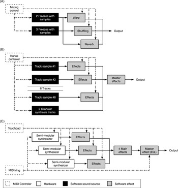
The three musicians – who I will name A, B and C from now on – use very different desktop management interfaces (DMIs) and devices (Figure 4). They have evolved considerably since the 1990s but have remained fairly stable over the three years of recording studied in this article.
Schematic diagram of the performance DMIs and devices of each musician (A, B and C).

Musician A uses a digital audio workstation (DAW; Pro Tools) with a mixing surface and mouse to control audio sample playback and transformations. Eleven effects are used to transform the samples: five parallel freeze plugins, two spectrum reordering effects (Warp), three shuffling effects and a reverb.
Musician B uses a DAW (Ableton Live) and a KarlaxFootnote 21 MIDI controller to play and transform audio samples positioned on eight tracks plus two granular synthesisers. The effects are numerous, are adapted to the various samples and can be combined: delay, spectral transposition, granular synthesis, temporal stretching or contraction, freeze, simple and resonant filters, reverb, vocoder, amplitude modulation and spatialisation.
Musician C uses three modular synthesisers as audio sources, a DAW (Ableton Live) for sound transformation and a touchpad as well as a MIDI ring for controlling transformations and synthesisers. There are quite a few transformations and they are customised for each of the three synthesisers. They are divided into four categories: delay, shuffling, spectrum transformation (by filtering, alteration or distortion) and amplitude modulation. Five output effects complete the sound transformation device: reverb, resonant filter, live granular synthesis, time filter and equalisation.
These devices are sometimes simple – as in the case of musician A – or more complex in their operation – as in the case of the other two musicians – but they are particularly effective in allowing a considerable richness of timbre. The control interfaces (mixing control, Karlax, touchpad, MIDI ring, synthesiser controls and patches) also offer many ways to interact live and anticipate the sound generated by the other musicians. The great difference between the three devices has encouraged each musician to develop a remarkably personal style of musical performance and to use very different strategies.
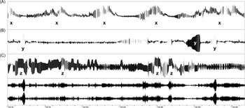
Figure 5 Footnote 22 illustrates this differentiation in a short 30-second excerpt. It contains four representations (from bottom to top): the waveform of the global mix and a BStD for each of the musicians computed on RMS amplitude (Y), spectral variance (width) and ZCR (colour). Musician A’s playing is characterised by a series of waves (x) that are found on the waveform of the global mix. Musicians B and C have an accompanying role, creating three specific moments (y) for B and accompanying some waves of A (z) with continuous playing for C. I chose this excerpt because the playing strategies of the three musicians represent an evident interaction with their DMI and devices: wide motions on the mixing control faders for A, sudden motions or triggers on the Karlax for B and fast and continuous motions with the MIDI ring for C.
BStD (A, B and C) based on RMS amplitude, spectral variance, ZCR; waveform on the global mix (Sound Example 1).

In this example, the BStD representation reveals an especially clear insight into the gestures of the musicians. The combination of the three descriptors reveals morphologies that are directly related to the devices and DMIs used by musicians.
4.2. The structure of time
The analysis of the structure of time of an improvised electroacoustic performance often reveals different strategies used by the musicians. The most common ones are a sequence of well-identified moments, a continuous development or a freeze of time without any evolution. Repetitions with or without variations, as found in works composed in the studio, are generally quite rare as they require preparation and are therefore partially composed. Even if the forms used are chosen from a somewhat limited stock, their realisation often appears to be difficult to analyse because there are multiple variations. Actually continuous present-type (continuous development) forms contain little information; it is thus necessary to relate them to the gestures as in the preceding example or to the microstructures presented at different levels. However, analysing a form in electroacoustics is always a challenge, as the structures can be complex and dense and the evolution of forms can be fast, sometimes even disordered.
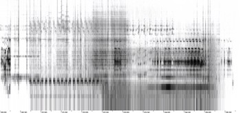
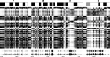
If the improvised performance is long, the memorisation of the form is very difficult; a visual support is thus essential. Logarithmic FFTFootnote 23 and similarity matrix are the most effective aids to form analysis. While the logarithmic FFT (Figure 6) provides a good visualisation of the spectral mass balance, a similarity matrix (Figure 8) will facilitate the analysis of the global form by leaving the microstructures visible. Figure 7 represents a self-similarity matrix of a complete improvised performance containing four sets separated by silences. The reading of the vertical bands will facilitate the formal segmentation (drawn on top). The comparison between the different vertical bands also provides some hypotheses about close moments in terms of timbre (e.g., those represented in the form of grey rectangles).
Logarithmic FFT representation of the global mix (Sound Example 2).

A self-similarity matrix computed on the FFT and a formal segmentation (top) of the four parts of the improvised performance.

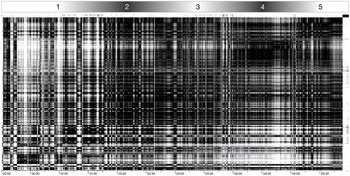
Self-similarity matrix computed on RMS amplitude, spectral rolloff, spectral variance and ZCR with segmentation in five zones on top (Movie Example 1).

The self-similarity matrix thus appears to be a fairly powerful formal segmentation tool. However, its interpretation can also be confusing. In Figure 8, I have used several descriptors to compute the self-similarity matrixFootnote 24 on the same audio source as in Figure 6. Five areas appear quite clearly in the matrix, the first being well differentiated from the others. On listening, the five zones are confirmed but also show a formal construction made up of subtle variations in timbre rather than of well-differentiated parts, as opposed to a purely visual interpretation based on vertical lines. The beginnings and ends of the zones are thus difficult to isolate even if the matrix seems to reveal quite precise formal segmentation. The difference between representation analysis and listening analysis is therefore very significant here.
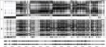
In Figure 9, the same phenomenon appears on another improvisation extract. On listening, as a whole the extract seems fairly uniform, the variations are progressive, and there is only one formal articulation at 0:51 with the emergence of a sound close to white noise with no variations in the rest of the sound material. This sound is then present until 7:09 almost to the end. The top matrix (1), computed from the FFT, shows some fine changes in the spectrum. The middle matrix (2), computed from a set of descriptors, reveals the continuous modification of the audio flux; it highlights the inserts made from a wide variety of materials around the white noise.
Two self-similarity matrices calculated from the FFT (1 at top of figure) and from the RMS amplitude, spectral rolloff, spectral variance and ZCR (2 at centre of the figure), and the waveform (bottom) (Movie Example 2).

These two extracts (Figures 6–8 and Figure 9) reveal two types of musical form. The first is based on a set of zones, focal points, which are difficult to isolate by listening. The second type is based on a continuity given by a single sound; the additions around this sound can change the material without really moving the musical discourse forward, a musical discourse that remains very static. Here the study of self-similarity matrices facilitates the identification and exemplification of form by guiding analytical listening. However, Figure 6 has shown that a study focused on visual representation generally causes errors of interpretation.
4.3. Musical strategies
In the previous example (Figure 9), the noisy material is due to one of the musicians, who is responsible for the stagnation of the form. During the improvisation, listening to the separate tracks, we realised that the other two musicians are constantly oscillating between two strategies: trying to break with the static of the noisy material and accompanying it. However, the two strategies are not really separately identifiable. This is one of the characteristics of free or electroacoustic improvisation: it is often difficult to isolate the musicians’ behaviour patterns. Even if the topic of a free improvisation can be fixed in advance, the path to implement it is never a straight line. The pleasure experienced by the listeners is also linked to the detours, the surprises, whether intended or not, and in the latter case, the listener is delighted with the way in which the musician will use this ‘good mistake’ to enrich the musical discourse. That is why I prefer to talk about strategies rather than behaviour. A strategy may be implicit; improvisers may not be aware of it, and it is only by listening to the improvised performance that they do become aware of it.
Under these conditions, how should the study of these strategies be approached and what are the elements to be taken into account? The first important element is to conduct a precise study of the instruments, devices and DMIs used by musicians. The development of a certain musical instrument responds to the musician’s intentions and, at the same time, has a strong influence on his performance. Thor Magnusson talks about the ergodynamism (Magnusson Reference Magnusson2019: 10–12) present in each instrument, that part of the instrument that is part of the culture, of a musical theory, of a more or less formalised artistic intention and that influences the musical rendering. In electroacoustic improvisation, musicians construct their instrument by assembling devices to comply with various constraints such as cultural adaptation or physical limitations, the stylistic objective of the improvisation, originality of timbre or of modes of play. In the latter case the aim may be to differentiate themselves from other musicians (or on the contrary for the purpose of homogeneity). Their instrument will also cater for the potential of play, including the potential of surprise, and the capacity to evolve (modularity). I previously described the three devices used in the improvisations analysed here. I started by showing how their differences lead to different strategies. Of course, the excerpts analysed are not representative of all of the group’s improvisations, and it would be very difficult to conduct a systematic study, but these considerations have allowed me to highlight methods of analysis and representation to focus the study on certain aspects of the musical excerpts.
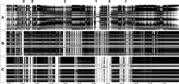
To conclude this study, I would like to show how it is possible to complete the study conducted previously by observation of similarity matrices computed on the FFTs of each musician’s audio file. In this extract of more than 12 minutes in Figure 10, at first sight the musicians’ playing appears to be clearly differentiated. Only two moments of synchronisation between the three are really identifiable during the performances (1); the other moments of synchronisation are realised only between two musicians (2). It is noticeable that these synchronisations are not always aligned; there is often one musician who leads off and is followed by one other or by both. Moreover, some breaks that are globally perceptible through hearing are realised by one musician only (e.g., in 3).
Three self-similarity matrices calculated for each musician on the FFT (Movie example 3).

The colours of the matrices also reveal some particularly interesting aspects. For example, musician A uses the faders on his console or the DAW interface to create smooth transitions. These transitions are visible in the progressive colour gradients. By comparison, musician C develops a more monolithic playing strategy, without progressive transitions, using only ruptures. Musician B develops a strategy somewhere in between, creating a link with the other musicians.
These analytical remarks have their origin in the graphical analysis of the representations. Listening to the global mix and the separate tracks of each musician has confirmed them.
5. Conclusion
In this article, I introduced the context and the development of a framework for the analysis of electroacoustic music. Applied to the analysis of improvisation, I demonstrated how descriptor extraction and data representation techniques could be useful for the musicologist. Improvisation is an ephemeral action, the study of which poses many problems regarding identification of elements and their analysis. Electroacoustic improvisation has two additional challenges: the complexity of sound materials and structures and the role of instrument development chosen by the musician in the performance. The purpose of the methods presented in this article is to offer the possibility of going beyond these difficulties and conducting analytical work on blurred, ephemeral, elusive objects – non-objects that are difficult to study with the classical techniques of musical analysis.