1. Introduction
Global surface temperature has risen notably, and recent decades have been considerably warmer than any earlier ones (IPCC, 2021). The Earth’s surface temperature was higher by 0.99°C during 2001–2020 and by 1.09°C during 2011–2020 relative to the base period 1850–1900 (IPCC, 2021). Forecasts indicate that global temperatures are expected to reach 1.5°C between 2030 and 2052 if the rate of increase continues at the current rate (IPCC, Reference Masson-Delmotte, Zhai, Pörtner, Roberts, Skea, Shukla, Pirani, Moufouma-Okia, Péan, Pidcock, Connors, Matthews, Chen, Zhou, Gomis, Lonnoy, Maycock, Tignor and Waterfields2018). Driven by climate change, the occurrence and severity of heatwaves have risen in most parts of the globe since the 1950s (IPCC, 2021).
Climate change has already resulted in numerous harmful effects, including increased health risks, more frequent droughts, food insecurity and adverse impact on overall economic outcomes (McMichael et al., Reference McMichael, Woodruff and Hales2006; Bosello et al., Reference Bosello, Roson and Tol2007; Dell et al., Reference Dell, Jones and Olken2014; Gosling and Arnell, Reference Gosling and Arnell2016). The global loss from extreme heat is estimated to range between $16 trillion and $50 trillion over the period 1992–2013 (Callahan and Mankin, Reference Callahan and Mankin2022). Climate change imposes a twofold burden on an economy: it undermines development outcomes and exacerbates disparities. Economies with low incomes, high agricultural dependence and hotter climates suffer most (Acevedo et al., Reference Acevedo, Mrkaic, Novta, Pugacheva and Topalova2020; Callahan and Mankin, Reference Callahan and Mankin2022). Several studies have established that climate change affects the poor disproportionately (Méjean et al., Reference Méjean, Collins-Sowah, Guivarch, Piontek, Soergel and Taconet2024). For instance, globally, poor people are less responsible for greenhouse gas emissions but often suffer more from their impact (World Bank, 2024). Climate change may entrap 35–122 million people in poverty by 2030 (Rozenberg and Hallegatte, Reference Rozenberg and Hallegatte2015). Furthermore, exposure to temperatures above a critical threshold is detrimental to health and adversely affects social outcomes (Carleton and Hsiang, Reference Carleton and Hsiang2016).
The effect of climate change on economic inequality has received considerable attention in the literature (Méjean et al., Reference Méjean, Collins-Sowah, Guivarch, Piontek, Soergel and Taconet2024). The present study adds to the body of knowledge developed by previous studies, including Dell et al. (Reference Dell, Jones and Olken2012, Reference Dell, Jones and Olken2014) and Hallegatte et al. (Reference Hallegatte, Bangalore, Bonzanigo, Fay, Kane, Narloch, Rozenberg, Treguer and Vogt-Schilb2016). The study builds on Paglialunga et al. (Reference Paglialunga, Coveri and Zanfei2022) who found that an increase in temperature exacerbates within-country inequality. However, owing to within-country heterogeneity, the present study analyses the impact of extreme heat on inequality at the district level in India.
The present study contributes in several ways. The existing literature tends to investigate the effects of extreme heat on inequality using national aggregates within cross-country frameworks (Diffenbaugh and Burke, Reference Diffenbaugh and Burke2019; Acevedo et al., Reference Acevedo, Mrkaic, Novta, Pugacheva and Topalova2020; Callahan and Mankin, Reference Callahan and Mankin2022). The effects of climate change are shaped by a variety of local factors, including geographic features, climatic conditions, the proportion of vulnerable populations, adaptability and the effectiveness of mitigation policies within a country. Hence, it is essential to examine the distributional effects of extreme heat within a country. Additionally, estimates at the country or aggregate level may underestimate climate risk (Dang et al., Reference Dang, Hallegatte, Nguyen and Trinh2026), particularly because they fail to account for the varying impacts of extreme heat across regions and populations within the country. Large countries such as India, with geographical and climatic diversity, demand subnational-level analysis of extreme heat and inequality. To the best of our knowledge, no study has examined the effect of heatwaves on inequality at the district level. This paper aims to fill this gap in the context of India. The present study contributes by investigating the effects of extreme heat, in terms of heatwaves, hot days and heat stress, on consumption inequality in India during the period 2014–2022 across more than 400 districts.
Extreme heat affects overall economic outcomes and gross domestic product (GDP), but it has a more direct effect on household consumption expenditure. Therefore, we used a bottom-up approach in which inequality is calculated from household-level consumption expenditure data. There is no universal consensus on a single index of heatwaves, given the varying strengths and limitations across indices. The study calculates and uses multiple indices of extreme heat, including heatwaves and hot days. Heat stress is also incorporated to provide a multifaceted understanding of extreme heat phenomena and their implications. Furthermore, we analyse the effect of extreme heat on inequality under varying temperature anomalies and agricultural intensity, emphasising the roles of adaptation and agriculture in this process.
The study does not rely on a single reference period and percentile to calculate the temperature reference value (TRV); instead, it uses multiple reference periods and percentiles. Rather than using average monthly or annual temperatures, we used hourly and daily temperature data to avoid bias from annual averages. We controlled for economic activity and other climate variables using high-resolution gridded data. The study used fixed-effects regression with clustered standard errors in the main analysis.
We employed multiple robustness checks. For precipitation, we used various indicators, including the annual mean precipitation, precipitation anomaly and the Standardised Precipitation Index (SPI). Both the generalised entropy measure and the Atkinson index with a varying sensitivity parameter are utilised to measure inequality for a robustness check. The study used fixed-effects regression with Colney spatial standard-error correction. The study also examined the dynamic nature of inequality using the Arellano–Bond generalised method of moments (GMM) dynamic panel model. We leveraged machine learning methods to examine the causal effect of extreme heat on inequality, employing the double machine learning framework.
The remainder of the paper is structured as follows. Section 2 presents a review of the literature. Section 3 describes the data sources and the variables used. Section 4 presents the conceptual framework. Section 5 outlines the methodology, including potential issues and remedies. Section 6 presents the results and discussion. Section 7 addresses robustness. Section 8 concludes with policy implications.
2. Literature review
2.1. Climate change and inequality: cross-country
The economic consequences of rising temperatures have been documented in numerous studies (Dell et al., Reference Dell, Jones and Olken2012, Reference Dell, Jones and Olken2014; Auffhammer, Reference Auffhammer2018; Diffenbaugh and Burke, Reference Diffenbaugh and Burke2019; Callahan and Mankin, Reference Callahan and Mankin2022). Previous studies have shown that the costs of rising temperature are distributed unevenly across countries. Energy consumption in developed economies substantially harms poorer economies through climate warming (Diffenbaugh and Burke, Reference Diffenbaugh and Burke2019), and the direct benefits of using fossil fuels are also distributed disproportionately (Diffenbaugh and Burke, Reference Diffenbaugh and Burke2019). Additionally, climate change vulnerability is greatest in poor countries. For instance, Cevik and Jalles (Reference Cevik and Jalles2023) found that climate change vulnerability is seven times higher in low-income countries. Alizadeh et al. (Reference Alizadeh, Abatzoglou, Adamowski, Prestemon, Chittoori, Asanjan and Sadegh2022) show that, over the past four decades, heatwave trends have been most pronounced in regions in the lowest income quartile, which experienced approximately 40% greater exposure than regions in the highest income quartile. Further, the adverse effects of rising temperatures on economic output are profound in hot-climate countries (Acevedo et al., Reference Acevedo, Mrkaic, Novta, Pugacheva and Topalova2020; Callahan and Mankin, Reference Callahan and Mankin2022). Climate change may impede progress in poverty alleviation by adversely affecting the agricultural sector (Hallegatte et al., Reference Hallegatte, Bangalore, Bonzanigo, Fay, Kane, Narloch, Rozenberg, Treguer and Vogt-Schilb2016). Countries with a larger proportion of vulnerable people are more exposed to climate change and further accelerate between-country inequality (Paglialunga et al., Reference Paglialunga, Coveri and Zanfei2022). Climate change vulnerability appears to have negligible effects in advanced economies, whereas its impact is substantially greater in developing countries due to limited adaptation and mitigation (Cevik and Jalles, Reference Cevik and Jalles2023).
Dell et al. (Reference Dell, Jones and Olken2012) identified the effects of historical temperature fluctuations on aggregate economic outcomes, showing that a 1℃ rise in temperature in a year results in a 1.3% decline in economic growth in poor economies. Diffenbaugh and Burke (Reference Diffenbaugh and Burke2019) found that it is highly probable that global warming has worsened economic inequality. Drawing on a systematic literature review, Méjean et al. (Reference Méjean, Collins-Sowah, Guivarch, Piontek, Soergel and Taconet2024) report that findings across multiple empirical studies confirm that the adverse effects of climate change are more pronounced among economically disadvantaged groups.
2.2. Climate change and inequality: within-country
The adverse effects of climate change on the lower-income group are likely to exceed the average impact, even within a country (Hallegatte and Rozenberg, Reference Hallegatte and Rozenberg2017). Rising temperatures impose relatively greater economic burdens on poor people, leading to more pronounced income declines and contributing to an expansion of the income gap. Paglialunga et al. (Reference Paglialunga, Coveri and Zanfei2022) investigated the effect of temperature on within-country income inequality across about 150 countries spanning 2003–2017 and found that a rise in temperature is positively associated with inequality. Zhao et al. (Reference Zhao, Liu, Piao, Wang, Lobell, Huang and Asseng2017) examined how climate change impacts poverty alleviation in China, India and Senegal, focusing on rural poor areas. Their findings reveal that climate change is closely linked to both agricultural performance and human welfare. Climate change affects poor people and poverty through various channels, including agriculture, natural disasters and health shocks (Hallegatte et al., Reference Hallegatte, Bangalore, Bonzanigo, Fay, Kane, Narloch, Rozenberg, Treguer and Vogt-Schilb2016).
2.3. Climate change and inequality: India
India has experienced increases in mean temperatures and the frequency of heatwaves, which are expected to continue rising (Rohini et al., Reference Rohini, Rajeevan and Srivastava2016). Previous studies have focused more on the effect of rising temperatures on overall consumption expenditure in India (Aggarwal, Reference Aggarwal2021). The existing literature documents the detrimental effects of excessive temperatures on agricultural yields and incomes in India (Burgess et al., Reference Burgess, Deschenes, Donaldson and Greenstone2014; Aggarwal, Reference Aggarwal2021). Climate change affects rural and urban regions differently. Burgess et al. (Reference Burgess, Deschenes, Donaldson and Greenstone2014) found that an increase in the number of extremely hot days reduces agricultural yields and wages and increases mortality in rural regions. Extreme heat reduces daily productivity and attendance among workers in the manufacturing segment of the Indian economy (Somanathan et al., Reference Somanathan, Somanathan, Sudarshan and Tewari2021). As far as adaptation is concerned, heat-prone regions in India tend to exhibit adaptation to elevated temperatures (Taraz, Reference Taraz2018). In heat-prone districts, economic losses from rising temperatures are relatively small compared with those in regions with lower heat (Taraz, Reference Taraz2018). Households also faced varying degrees of exposure to changes in food prices driven by climate change. Urban households are more reliant on buying food than rural households and therefore face relatively greater losses from rising food prices (Jacoby et al., Reference Jacoby, Rabassa and Skoufias2011).
3. Conceptual framework
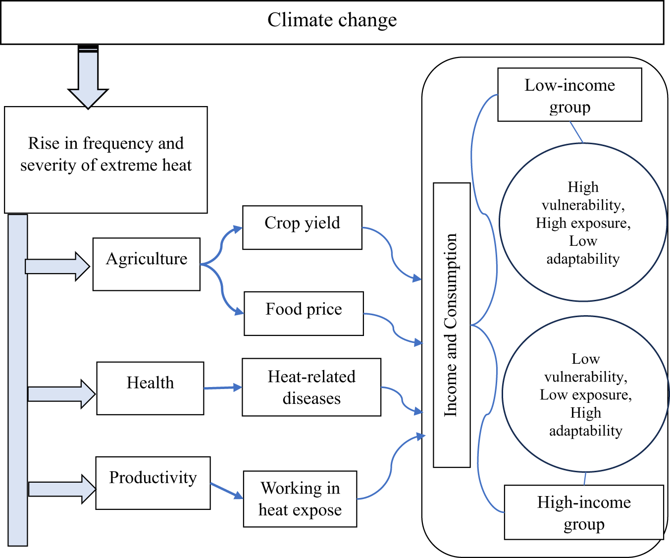
From the existing literature, we identified three major channels, namely, agriculture, health and productivity, through which extreme heat affects the distribution of consumption expenditure (Figure 1). However, these channels are not independent but are intrinsically interrelated. The extent of reliance on agriculture within an economy is an important mechanism through which weather shocks affect income and consumption distribution (Hallegatte et al., Reference Hallegatte, Bangalore, Bonzanigo, Fay, Kane, Narloch, Rozenberg, Treguer and Vogt-Schilb2016; Acevedo et al., Reference Acevedo, Mrkaic, Novta, Pugacheva and Topalova2020; Paglialunga et al., Reference Paglialunga, Coveri and Zanfei2022; Palagi et al., Reference Palagi, Coronese, Lamperti and Roventini2022). In agriculturally intensive countries, a large proportion of poor people rely on agriculture; consequently, climate anomalies disproportionately reduce incomes for the lower-income group and generate greater income disparity (Palagi et al., Reference Palagi, Coronese, Lamperti and Roventini2022). Rainfall variability and agricultural dependence are key determinants when estimating the climate-related impacts on poorer segments of the population (Palagi et al., Reference Palagi, Coronese, Lamperti and Roventini2022). Crop yields and food prices are sensitive to extreme heat, with a relatively greater negative effect on farmers, rural communities and the poor (Biewald et al., Reference Biewald, Lotze-Campen, Otto, Brinckmann, Bodirsky, Weindl, Popp and Schellnhuber2015; Hallegatte et al., Reference Hallegatte, Bangalore, Bonzanigo, Fay, Kane, Narloch, Rozenberg, Treguer and Vogt-Schilb2016; Zhao et al., Reference Zhao, Liu, Piao, Wang, Lobell, Huang and Asseng2017). Extreme heat reduces agricultural output, lowers the productivity of those who work outdoors, slows investment and increases heat-related health issues (Acevedo et al., Reference Acevedo, Mrkaic, Novta, Pugacheva and Topalova2020). Heatwaves decrease the productivity of outdoor labour (Kjellstrom et al., Reference Kjellstrom, Holmer and Lemke2009) and also reduce workers’ productivity and attendance in the manufacturing sector (Somanathan et al., Reference Somanathan, Somanathan, Sudarshan and Tewari2021).
Conceptual framework of extreme heat and distributional impacts.

1 Long description
The diagram shows the impact of climate change, specifically the rise in frequency and severity of extreme heat. There are three main channels: agriculture, health, and productivity. In agriculture, extreme heat impacts crop yield and food prices. In health, it leads to heat-related diseases. In productivity, it affects the productivity of workers working in heat exposure. These factors influence income and consumption, particularly affecting low-income and high-income groups differently. The low-income group is characterized by high vulnerability, high exposure and low adaptability, while the high-income group has low vulnerability, low exposure and high adaptability.
4. Data and variable description
4.1. Inequality
This study uses data from the Consumer Pyramid Household Survey (CPHS) for the period 2014–2022. The CPHS, conducted by the Centre for Monitoring Indian Economy (CMIE), is a panel household survey covering approximately 170,000 households, more than 400 districts, and all major states of India.Footnote 1 The CPHS provides household-level monthly consumption expenditures for various items, including food and non-food. We used adjusted monthly consumption, which is more reliable because it is derived from weekly expenses. To calculate per capita consumption expenditure, we used household size information for each month. For households situated in rural (urban) areas, the rural- Consumer Price Index (CPI) (urban-CPI) is used to calculate real monthly per capita consumption expenditure (MPCE). The final variable used to calculate inequality is real MPCE. We rely on household consumption expenditure rather than income to measure inequality because of limitations associated with household income data (Deaton, Reference Deaton2018). We employed the Gini coefficient to quantify inequality in MPCE for each district and year:
 \begin{equation}\text{Gini}{\,_{\text{dis},\,y}} = \,\frac{1}{{2{n^2}\mu }}\mathop \sum \limits_i^n \mathop \sum \limits_j^n \left| {{\text{MPCE}_{i,\text{dis},y}} - {\text{MPCE}_{j,\text{dis},\,y}}} \right|.\end{equation}
Here,  $\text{dis}$ stands for district,
 $i$ and
 $j$ for households and
 $\mu $ for mean MPCE. In measuring inequality, the Gini coefficient gives more weight to the middle of the distribution. Therefore, for robust analysis, we used the generalised entropy class of measures and the Atkinson index, allowing for different sensitivity parameters (see Description A1 in the Supplementary Appendix). All these indices are also calculated with the same variable, namely MPCE, from CMIE.
4.2. Weather variables
The analysis of extreme heat and inequality relies on metrics including heatwaves, hot days and heat stress. Weather variables, namely precipitation and humidity, affect inequality and are therefore included in the model (Palagi et al., Reference Palagi, Coronese, Lamperti and Roventini2022; Dang et al., Reference Dang, Hallegatte, Nguyen and Trinh2026).
4.2.1. Heatwaves
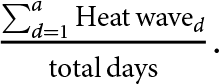
We utilised the high-resolution daily gridded temperature data for the period 1979–2022. The data source is the global unified temperature data made available by the Physical Sciences Laboratory of the National Oceanic and Atmospheric Administration (NOAA). It provides daily temporal resolution with a 0.50° latitude and longitude grid.Footnote 2 We calculated the annual proportion of heatwaves for all districts.Footnote 3
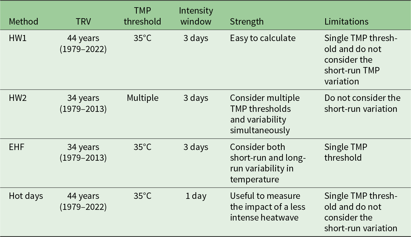
According to the India Meteorological Department (IMD), a heatwave is a period when temperatures are higher than usual for a particular region. More specifically, a heatwave is defined as occurring when the daily mean temperature exceeds the pth percentile of the local annual mean daily temperature in a reference period for at least ‘k’ consecutive days (Rohini et al., Reference Rohini, Rajeevan and Srivastava2016; Alizadeh et al., Reference Alizadeh, Abatzoglou, Adamowski, Prestemon, Chittoori, Asanjan and Sadegh2022). However, there is no universal definition or set of measurement criteria for calculating the heatwave index. Therefore, this study incorporates a wide range of methods for measuring heatwaves. Table 1 summarises the heatwave indices used in this study.
Summary table of various heatwave methods

Table 1 Long description
HW1 uses 44 years of data, a single 35 degrees C threshold, and a 3-day window; it is easy to calculate but does not capture short-term temperature variation. HW2 uses 34 years, multiple thresholds, and a 3-day window; it captures multiple thresholds and variability together but still omits short-term variation. EHF uses 34 years, a single 35 degrees C threshold, and a 3-day window; it considers both short-term and long-term temperature variability, but it relies on a single threshold. Hot days uses 44 years, a single 35 degrees C threshold, and a 1-day window; it is intended for less intense events but does not include short-term variation.
Source: Authors’ representation.
A 3-day window and a 35°C criterion are used, which are suitable for the Indian subcontinent (Rajeevan et al., Reference Rajeevan, Rohini, Nair, Tirkey, Goswami and Kumar2023). The technical explanation of each method is provided below.
Method 1: The heatwave is calculated in two steps following Rohini et al. (Reference Rohini, Rajeevan and Srivastava2016). First:
 \begin{equation}\text{H}{1_{\text{dis},d}} = \begin{cases}
{1,\, {\text{if}\,{\text{TMP}_{\text{dis},y,\,\,m,d}} \gt 35} {\text{ and}\,{\text{TMP}_{\text{dis},y,m,d}} \gt \,\text{TRV}_{\text{dis},m,d}^{p90}}} \\
{0,\,\, {\text{otherwise}}}
\end{cases},\end{equation}
where H1 represents the heatwave condition calculated using method 1.  ${\text{TMP}}$ is the temperature,
 ${\text{TRV}}$ is the temperature reference value,
 $i$ represents the district,
 $y$ is the year,
 $m$ is the month and
 $d$ is the day.
 $p{\text{90}}$ is the 90th percentile of the
 ${\text{TRV}}$. After identifying a heatwave condition in Equation (1), the second step calculates the heatwaves as
 \begin{equation}\text{HW1}_{\text{dis},\,d}^{k = 3} = \begin{cases}
{1,\,\,\,\text{if}\,\mathop \sum \limits_{j = 0}^{k - 1} \text{H}{1_{\text{dis},d - j\,}} \geqslant k} \\
{0,\,\,\text{otherwise}}
\end{cases}.\end{equation}
A heatwave in the district occurs when the temperature on a given day exceeds 35°C and the 90th percentile of the TRV (Equation (2)), and when this condition persists for 3 consecutive days (Equation (3)). Following this process, we calculated the annual proportion of heatwaves for each district.Footnote 4
Method 2: Usual temperatures vary across regions, including hilly, plain and coastal districts. A single temperature threshold cannot capture these differences among districts. To avoid this bias, we used the IMD definition, with varying thresholds, to calculate heatwaves. The second heatwave index (HW2) calculation involves the following two steps. First,
 \begin{equation}\text{base}\,\text{TMP}_{\text{dis},d,m} = \,\frac{1}{{34}}\mathop \sum {\text{TMP}_{\text{dis},d,m,y\,}}.\end{equation}
The temperature variability is calculated using the following equation:
 \begin{equation}\text{TMP}\ \text{variablity} = {\text{TMP}_{\text{dis},d,m,y}} - \text{base}\,{\text{TMP}_{\text{dis},d,m}}.\end{equation}
Following the IMD basic criterion and involving multiple cut-offs with the combination of temperature and variability, the second step is:
 \begin{align}
&\text{H2} =\left\{\begin{array}{@{}l@{}}
1,\,\text{if}\ \text{TMP}_{\text{dis},d,m,y}\,\,\,\,\,\,\,\,\,\,\,\,\,\,\,\, \gt \,\,\text{40}\ \text{and}\ \text{TMP}\ \text{variablity}\,\, \gt \,2, \nonumber \\
1,\,\text{if}\ 37 \geqslant \text{TMP}_{\text{dis},d,m,y}\,\, \lt \,\,\text{40}\,\text{and}\ \text{TMP}\ \text{variablity}\,\, \gt \,\,5, \nonumber \\
1,\,\text{if}\ 35 \gt \,\text{TMP}_{\text{dis},d,m,y}\,\, \lt \,\,\text{37}\,\text{and}\ \text{TMP}\ \text{variablity}\,\, \gt \,\,7, \nonumber \\
0,\,\,\text{otherwise}\, \nonumber \\
\end{array}\right.. \nonumber \\
&\text{HW2}_{\text{dis},\,d}^{k = 3} =\begin{cases}
{1,\,\,\,\text{if}\,\mathop \sum \limits_{j = 0}^{k - 1} \text{H}{2_{\text{dis},d - j\,}} \geqslant k} \\
{0,\,\,\text{otherwise}}
\end{cases}.
\end{align}
Method 3: Following the IMD, we calculated the Excess Heat Factor (EHF), a composite of two indices: the Excess Heat Index (EHI) and Heat Stress Index (HSI). The EHI is calculated as follows:
 \begin{equation}{\text{EHI}} = { }\frac{{{\text{TMP}_t} + {\text{TMP}_{t - 1}} + \,{\text{TMP}_{t - 2}}}}{3} - {\text{TRV}_p},\end{equation}
where the first part of the RHS of the formula is the 3-day average of temperature, and the second part is the TRV for the climate reference period 1979–2013, with the 97th percentile (Alizadeh et al., Reference Alizadeh, Abatzoglou, Adamowski, Prestemon, Chittoori, Asanjan and Sadegh2022) of  ${\text{TM}}{{\text{P}}_t}$.
The HSI is defined as follows:
 \begin{equation}{\text{HSI}} = { }\frac{{{\text{TMP}_t} + {\text{TMP}_{t - 1}} + \,{\text{TMP}_{t - 2}}}}{3} - \,\,\,\,\frac{{{\text{TMP}_{t - 3}} + \ldots + \,{\text{TMP}_{t - 32}}}}{{30}}\,.\end{equation}
Then, EHF is defined as
 \begin{equation}\text{EHF} = \,{\text{EHI*Max}}\left( {1,{\text{ HSI}}} \right)\end{equation}
 \begin{equation}\text{H}{3_{\text{dis},\,d}} = \begin{cases}
{1,\,\,\,\text{if}\,\,{\text{TMP}_{\text{dis},\,\,y,m,\,d}} \gt 35\,\text{and}\,\text{EHF} \gt 0,} \\
{0,\,\,\text{otherwise}}
\end{cases}\end{equation}
 \begin{equation}\text{HW3}_{\text{dis},\,d}^{k = 3} = \begin{cases}
{1,\,\,\,\text{if}\,\mathop \sum \limits_{j = 0}^{k - 1} \text{H}{3_{\text{dis},d - j\,}} \geqslant k} \\
{0,\,\,\text{otherwise}\,\,.}
\end{cases} \end{equation}
Method 4: This method is similar to Method 1, but it uses a 1-day window to define a heatwave instead of a 3-day window. In this case, we call it a hot day. It provides the flexibility to measure the effect of extreme heat on inequality using a lower-intensity or shorter-duration heatwave.
 \begin{equation}{\text{HD}_{\text{dis},\,d}} = \begin{cases}
{1,\,\,\,\text{if}\,\,{\text{TMP}_{\text{dis},\,\,y,m,\,d}} \gt 35\,and\,{\text{TMP}_{\text{dis},y,m,d}} \gt \text{TRV}_{\text{dis},\,m,\,d}^{p99}} \\
{0,\,\,\text{otherwise}}
\end{cases}\end{equation}
Temperature anomaly. Departure from the long-term temperature is considered a temperature anomaly. The normal or usual long-term temperature varies across districts. Departures and fluctuations from long-term temperature trends influence the impacts of and adaptability to heatwaves. We used a longer period for the reference temperature value or base temperature. The study uses the Climate Research Unit (CRU) monthly temperature data to compute the temperature anomaly. We used CRU TS v. 4.07, a gridded dataset covering the period 1901–2022 at 0.5° resolution. Using a 100-year (1901–2000) climate reference period, we calculated the temperature anomaly.Footnote 5
4.2.2. Heat stress
We used the human biometeorological index, the Universal Thermal Climate Index (UTCI), to explore the impact of heat stress on consumption inequality. The UTCI is intended as a unidimensional quantity that represents the human physiological response in a multidimensional real outdoor environment (Bröde et al., Reference Bröde, Fiala, Błażejczyk, Holmér, Jendritzky, Kampmann, Tinz and Havenith2012). The UTCI is defined as the temperature of a reference environment that would produce the same physical responses, such as sweat production, shivering, skin wettedness, skin blood flow and rectal, mean skin and face temperatures, under the actual conditions (Di Napoli et al., Reference Di Napoli, Pappenberger and Cloke2018). The UTCI combines air temperature, wind, radiation and humidity, reflecting the human body’s reaction to a particular combination. Therefore, alongside heatwaves, we used heat stress to examine its impact on consumption inequality, as it is directly associated with productivity loss during outdoor work. We used ERA5-HEAT (Human Thermal Comfort), a bioclimatology data record production. This is gridded data with 0.25° × 0.25° horizontal resolution, and horizontal coverage is the entire globe except Antarctica (90 N–60 S, 180 W–180 E). The database is organised into 24-hour files, covering the full day (00-23 UTC). UTCI is classified into 10 categories based on the intensity of heat stress (Błażejczyk et al., Reference Błażejczyk, Baranowski and Błażejczyk2014). We calculated the hours per day under ‘very strong’ heat stress and summed them over a year for each district.
4.2.3. Precipitation and humidity
We used precipitation and humidity to control for local weather conditions at the district level. The CRU monthly precipitation and humidity data from 1901 to 2022 are used. We mainly derived the precipitation anomaly and the SPI, along with the annual mean of precipitation, to control for the impact of extreme precipitation on inequality. The precipitation anomaly is calculated in a manner similar to the temperature anomaly. SPI is a probability index that measures abnormal wetness and dryness. According to the World Meteorological Organisation (2012), the time length of precipitation data should be at least 30 years. The SPI can be calculated with temporal scales of 3, 6 and 12 months. Following Paglialunga et al. (Reference Paglialunga, Coveri and Zanfei2022), we also derived one binary variable from SPI. The dummy variable is assigned a value of 1 when the ratio of SPI to the mean of the previous 10 years’ SPI is greater than 1; otherwise, 0.
4.3. Night-time light
The level of economic activity in a district may affect inequality within that district. District-level GDP data are unavailable for the study period. Therefore, the study uses night-time light (NTL) as a proxy for the district’s GDP to control for district-level economic activity.
The district-level GDP data from the District Level Database were made available for 2013 only by the International Crops Research Institute for the Semi-Arid Tropics. We used it to examine whether NTL can serve as a good proxy for GDP or income at the district level (see Supplementary Appendix Tables A1 and A2). The NTL data are drawn from the Earth Observation Group (Payne Institute) for the period from 2013 to 2021. Elvidge et al. (Reference Elvidge, Zhizhin, Ghosh, Hsu and Taneja2021) explain that the annual night light data are a product of monthly cloud-free radiance averages constructed from low-light imaging day/night band (DNB). The NTL data are collected by the National Aeronautics and Space Administration/NOAA Visible Infrared Imaging Radiometer Suite (VIIRS). The monthly DNB cloud-free composites are produced by averaging the radiance from orbital segments that are free of sunlight, moonlight and cloudy data based on the VIIRS cloud mask. We used version 2.1 of VNL.Footnote 6
5. Methodology
Potential biases and remedies. Economic activity may affect the distribution of consumption expenditure. The existing literature established that NTL is a good proxy for electricity consumption, urbanisation, industrialisation, migration (Niedomysl et al., Reference Niedomysl, Hall, Archila Bustos and Ernstson2017), GDP and, therefore, overall economic activity. We also established at the district level in India that NTL is strongly associated with GDP. Therefore, we used NTL data at the district level to control for overall economic activity. Districts of India are diverse in terms of geographical and other features, which may affect the distribution of consumption expenditure. District fixed-effect  $({\delta _i})$ captures fixed spatial characteristics, time-invariant district-level differences such as geography, and controls for potential omitted-variable bias and endogeneity (Dell et al., Reference Dell, Jones and Olken2014; Callahan and Mankin, Reference Callahan and Mankin2022). We also included the year fixed-effect, which controls for economic and climate shocks (Callahan and Mankin, Reference Callahan and Mankin2022). We control for other weather variables, namely precipitation and relative humidity, which may affect inequality levels. To examine the homoscedasticity assumption, we used the modified Wald test for group-wise heteroscedasticity in the fixed-effects regression model (see Supplementary Appendix Table A3). We calculated the robust standard error in the presence of heteroscedasticity in the model. Standard errors are clustered at the district level to facilitate potential serial correlation within a district over time. We additionally employ the Conley standard error (Conley, Reference Conley1999) to mitigate potential bias arising from spatial correlation.Footnote 7
If the assumption of exogeneity does not hold, there will be bias in the estimates. There are potential sources of endogeneity in the model. If a shock affects a district's inequality level in a given year, which may correlate with the future value of inequality, the error terms will be correlated over time (Paglialunga et al., Reference Paglialunga, Coveri and Zanfei2022). The inclusion of a lagged dependent variable 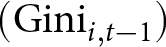 $({\text{Gin}}{{\text{i}}_{i,t - 1}})$ as a regressor tends to bias the coefficient estimation in short panelsFootnote 8 (Nickell, Reference Nickell1981; Dell et al., Reference Dell, Jones and Olken2014). This endogeneity issue, as explained by Nickell (Reference Nickell1981), is known as the Nickell bias. To address potential endogeneity, we used the Arellano and Bond (Reference Arellano and Bond1991) GMM.Footnote 9 However, it is important to note that GMM does not necessarily improve estimation. We have a short panel (T < 10). Including lags in the short panel increases the risk of biased estimation (Dell et al., Reference Dell, Jones and Olken2014). Given this risk and following Dell et al. (Reference Dell, Jones and Olken2014) and Paglialunga et al. (Reference Paglialunga, Coveri and Zanfei2022), we prefer Ordinary Least Squares (OLS) fixed-effects for the main analysis.
Weather variables may have complex associations with one another, including nonlinearities in the covariates and interactions. To control or minimise biases arising from the potential model misspecification and to leverage the power of machine learning to assess the causal effect of extreme heat on inequality, we used the double machine learning framework.
5.1. Econometrics analysis
5.1.1. Fixed-effects
We have a short-panel data structure (N > T), and the districts are diverse. Therefore, the fixed-effects panel model is the preferred choice for the analysis. Furthermore, using the Hausman test, we found that the fixed-effects model is appropriate for analysing extreme heat and inequality (see Supplementary Appendix Tables A4–A6). The linear form of the model is given below, with a two-way effect: district and year:
 \begin{equation}Gin{i_{it}} = \,{\beta _1}E{H_{it}} + \,\,\,{\beta _2}ln\left( {pr{e_{it}}} \right) + {\beta _3}{\text{ln}}(NT{L_{it - 1}}) + {\beta _4}ln\left( {HU{M_{it}}} \right)\, + {\delta _i} + \,{\gamma _t} + \,{\varepsilon _{it}}\,,\,\end{equation}
where  ${\text{EH}}$ represents extreme heat, which includes heatwaves (HW1, HW2, EHF), hot days and heat stress.
 ${\text{pre}}$ is precipitation, NTL is night-time light and HUM is humidity.
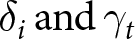 ${\delta _i}\,{\text{and}}\,{\gamma _t}$ are the district and year effects, respectively. To avoid multicollinearity among alternative measures of extreme heat, Equation (11) is estimated in five different models using EH as HW1, HW2, EHF, hot days (HD) and heat stress (HS). Heat stress incorporates relative humidity and temperature in the calculation; therefore, when estimating the model with heat stress, we have not used humidity and temperature separately as covariates. To control the local temperature condition, we introduced an interaction term into the model,
 \begin{align}Gin{i_{it}} &= \,{\beta _1}E{H_{it}} + {\beta _1}\left( {E{H_{it}}*TMP\,A{\,_{it}}} \right) + {\beta _2}ln\left( {pr{e_{it}}} \right) + {\beta _3}{\text{ln}}(NT{L_{it - 1}}) \nonumber\\
&\quad + {\beta _4}ln\left( {HU{M_{it}}} \right) + {\delta _i} + {\gamma _t} + \,{\varepsilon _{it}}\,,\,\end{align}
where TMP A represents the temperature anomaly.
5.1.2. Adaptation
For a detailed analysis of adaptation, we defined and classified the districts into high- and low-temperature anomaly groups:
 \begin{align}Gin{i_{it}}& = \,{\beta _1}E{H_{it}} + \,{\beta _1}\left( {E{H_{it}}*High\,TMP\,A{\,_{it}}} \right) + \,\,{\beta _2}ln\left( {pr{e_{it}}} \right) + {\beta _3}{\text{ln}}(NT{L_{it - 1}}) \nonumber\\
&\quad + {\beta _4}ln\left( {HU{M_{it}}} \right) + {\delta _i} + \,{\gamma _t} + \,{\varepsilon _{it}}\,\end{align}
A district is categorised as a high- (low-) anomaly district when its local temperature anomaly (calculated from long-term temperature) is above (below) the median.
5.1.3. Agriculture channel
 \begin{align}Gin{i_{it}} &= \,{\beta _1}E{H_{it}} + \,{\beta _1}\left( {E{H_{it}}*High\,Agri{\,_{it}}} \right) + \,\,{\beta _2}ln\left( {pr{e_{it}}} \right) + {\beta _3}{\text{ln}}(NT{L_{it - 1}}) \nonumber\\
&\quad + {\beta _4}ln\left( {HU{M_{it}}} \right)\, + {\delta _i} + \,{\gamma _t} + \,{\varepsilon _{it\,\,\,\,\,}}\,\,\,\,\,\,\,\,\,\,\,\,\,\,\,\,\,\end{align}
Districts are classified as high or low in agricultural intensity based on the proportion of cultivators and agricultural labourers to total labour.Footnote 10
5.1.4. Dynamic panel model
The following equation is the base (level) equation for the dynamic panel model:
 \begin{equation}Gin{i_{it}} = {\beta _1}Gin{i_{i,t - 1}} + {\beta _2}E{H_{it}} + {\beta _3}ln\left( {pr{e_{it}}} \right) + {\beta _4}{\text{ln}}(NT{L_{it - 1}}) + {\beta _4}ln\left( {R{H_{it}}} \right) + {\delta _i} + \,{\gamma _t} + {\varepsilon _{it}}.\end{equation}
All the notations are the same as explained above. 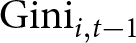 ${\text{Gin}}{{\text{i}}_{i,t - 1}}$ exhibits the dynamic nature of the equation. We performed the post-estimation test, namely the Arellano–Bond test for serial correlation in the error term and the Sargan and Hansen test of over-identification restrictions.
5.2. Double machine learning approach
We leveraged the debiased/double machine learning (DML) causal inference framework.Footnote 11 DML combines a non-parametric approach from machine learning models with a causal inference technique from econometrics (Chernozhukov et al., Reference Chernozhukov, Chetverikov, Demirer, Duflo, Hansen, Newey and Robins2018). The DML framework enables the quantification of treatment (or causal) effects using fixed-effect in a panel data setting. We estimated the causal effect of extreme heat on inequality while controlling for confounders. The study defines extreme heat as a treatment variable, and the previously defined covariates are cofounders. The partially linear model (Robinson, Reference Robinson1988) is defined as
 \begin{equation}Inequality = \left( {EH} \right)\emptyset + \left( X \right)\varphi + \, \in ,\,\,\,\,\mathbb{E}{\text{(}}\,\,\, \in {\text{|}}X,\,EH) = 0,\end{equation}
 \begin{equation}EH = \,\left( X \right)\psi + \,\varsigma \,,\,\,\,\mathbb{E}\left( {\varsigma \,{\text{|}}X} \right) = 0.\end{equation}
All notations are the same as previously defined.  $X$ is a vector of confounding covariates, and
 $ \in \,$ and
 $\varsigma \,$ are stochastic errors. Given the panel structure of the data, we used partially linear panel regression (PLPR) models (Clarke and Polselli, Reference Clarke and Polselli2026), which take the form:
 \begin{equation}Inequalit{y_{it}} = \left( {E{H_{it}}} \right){\emptyset _0} + \left( {{X_{it}}} \right){\varphi _1} + \delta _i^* + \,{ \in _{it}}\,,\,\,\,\,\,\mathbb{E}\,\left( {{ \in _{it}}{\text{|}}{X_{it}},\,\,E{H_{it}},\,\,\delta _i^*} \right) = 0,\,\end{equation}
 \begin{equation}E{H_{it}} = \,\left( {{X_{it}}} \right){\psi _1} + \,{\xi _i} + {\varsigma _{it}}\,,\,\,\,\,\,\,\,\,\,\,\,\,\,\,\,\,\,\,\,\,\,\,\,\,\,\,\,\,\,\mathbb{E}\left( {{\varsigma _{it}}{\text{|}}{X_{it}},\,{\xi _i}\,} \right) = 0,\end{equation}
where  $\,\delta _i^*$ and
 ${\xi _i}$ are unobserved individual heterogeneity terms. Clarke and Polselli (Reference Clarke and Polselli2026) strongly recommend adopting an ensemble strategy involving multiple learners in the empirical estimation. We used Random Forest, Neural Network, Ridge and Lasso as learners. DML PLPR allows for possible serial correlation within each unit, which is often the case for panel data (Clarke and Polselli, Reference Clarke and Polselli2026). Furthermore, district-level clustered robust standard errors are employed. We consider the first-difference transformation approach of PLPR, which is recommended by Clarke and Polselli (Reference Clarke and Polselli2026) and consistent with fixed-effects regression analysis.
6. Results and discussion
6.1. Descriptive statistics
Indian districts differ in the number of heatwaves experienced annually (see Supplementary Appendix Figure A1, panels B and C). Panel B demonstrates the intensity of EHF across districts in 2022. The central and northern regions of India experience a higher incidence of heatwaves. A similar spatial distribution of heatwaves is observed in a previous study (Rohini et al., Reference Rohini, Rajeevan and Srivastava2016). Panel D shows a skewed distribution of NTL intensity, and panel A shows the inequality level by district in India in 2022. The skewed distribution of heatwaves, inequality level and economic activity suggests the importance of the district-level analysis in India. Our results indicate pronounced inequality, with the Gini coefficient reaching 0.50 while the national average for India over 2014–2022 stands at 0.20 (see Supplementary Appendix Table A8). A similar level of inequality is found in a previous study (Verma et al., Reference Verma, Sahoo and Ghosh2023). The proportion of hot days in a year is higher than that of heatwaves because it is based on a day window rather than 3 days.
6.2. Regression results
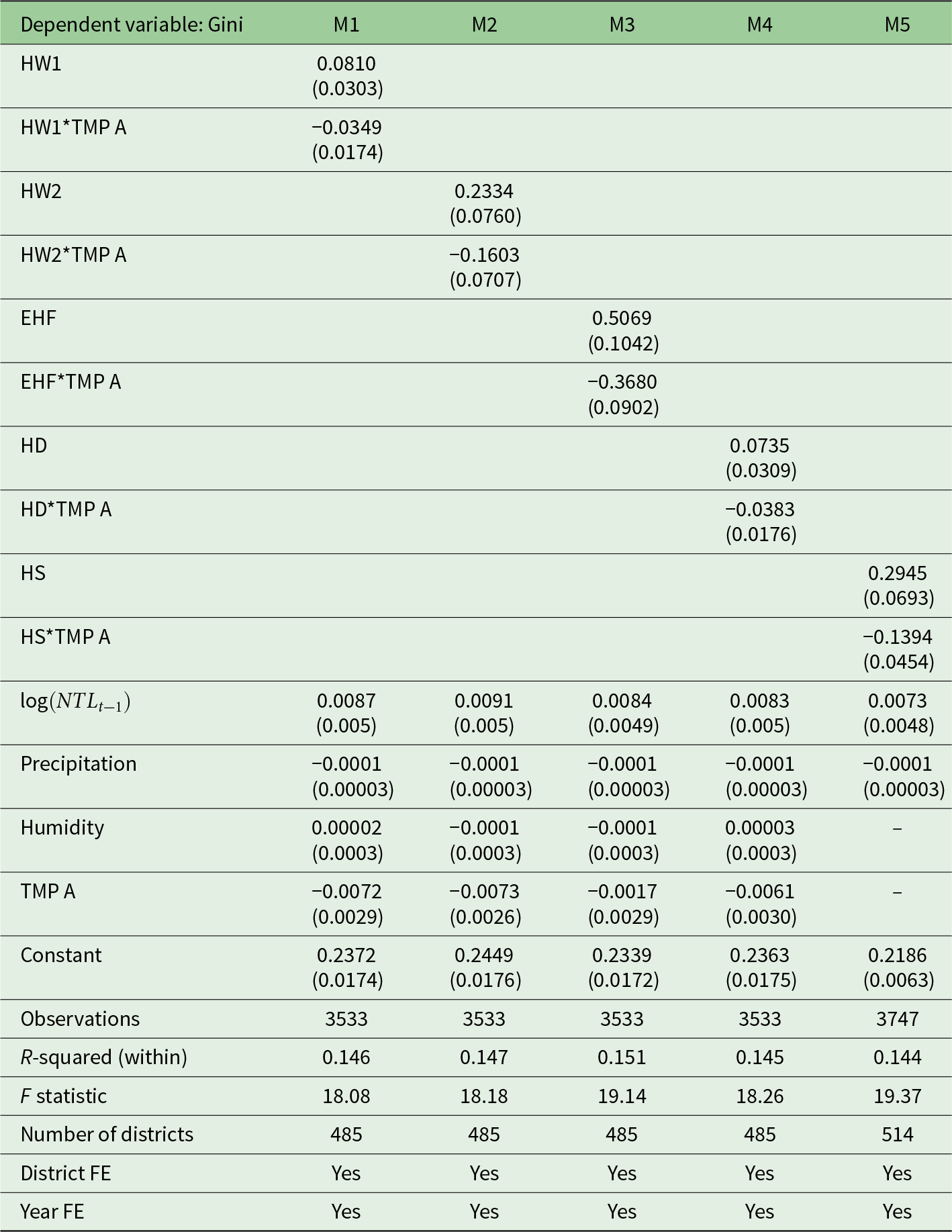
Heatwaves: After controlling for local weather conditions and district-level economic activity, we find a statistically significant effect of heatwaves on inequality (Table 2, Models 1, 2 and 3). Positive coefficients indicate that heatwaves adversely affect the distribution of MPCE. Regarding the magnitude of the effect, a 1% increase in heatwaves (measured by EHF) increases the Gini index by 0.5 percentage points. The effect of rising temperatures on the poor is expected to be more severe than the national average, even within the country (Hallegatte and Rozenberg, Reference Hallegatte and Rozenberg2017). Jessoe et al. (Reference Jessoe, Manning and Taylor2018) found that in Mexico, an increase in the number of heatwaves was associated with a decrease in local employment, particularly among daily-wage and non-agricultural workers.
Effect of extreme heat on inequality using fixed-effects regression
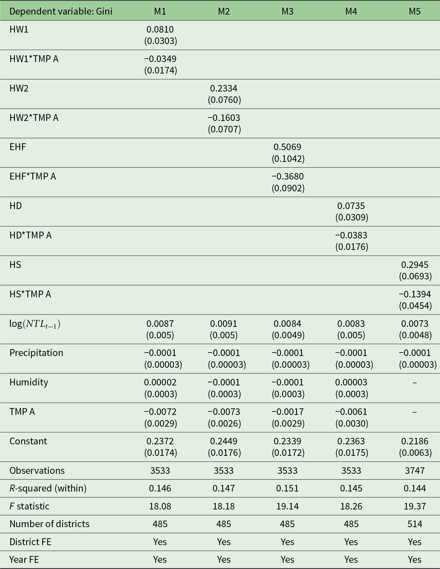
Table 2 Long description
The table reports district and year fixed-effects regression results with the Gini coefficient as the outcome and extreme-heat index as the explanatory variable. In model 1, HW1 is positively associated with inequality (0.0810), while its interaction with temperature anomaly is negative (-0.0349). In model 2, HW2 is positive (0.2334) and its interaction with average temperature is negative (-0.1603). In model 3, EHF is positive (0.5069) and its interaction is negative (-0.3680). In model 4, HD is positive (0.0735) and its interaction is negative (-0.0383). In model 5, HS is positive (0.2945) and its interaction is negative (-0.1394). Controls include lagged night-time lights, precipitation, humidity, and temperature anomaly. Sample sizes are 3,533 observations in models 1 to 4 and 3,747 in model 5, with within R-squared around 0.144 to 0.151. Standard errors are clustered at the district level.
Source: Authors’ calculations.
Note: District-level clustered standard errors in parentheses.
Three channels identified in the conceptual framework can explain how heatwaves affect inequality. Poor people are more exposed to the impacts of climate change in certain ways (Hallegatte et al., Reference Hallegatte, Bangalore, Bonzanigo, Fay, Kane, Narloch, Rozenberg, Treguer and Vogt-Schilb2016, Reference Hallegatte, Fay and Barbier2018). They are employed in sectors with relatively high heat exposure, such as construction and agriculture (Shonkoff et al., Reference Shonkoff, Morello-Frosch, Pastor and Sadd2011). A range of factors contribute to poor people’s vulnerability to heatwaves. They are more likely to be affected by rising food prices and greater dependence on income from the agricultural sector (Hallegatte et al., Reference Hallegatte, Bangalore, Bonzanigo, Fay, Kane, Narloch, Rozenberg, Treguer and Vogt-Schilb2016). For instance, Biewald et al. (Reference Biewald, Lotze-Campen, Otto, Brinckmann, Bodirsky, Weindl, Popp and Schellnhuber2015) found that in low-income countries, 56% of the global population may face rising food costs in 2030 and 73% in 2080 due to climate change. According to the Economic Survey 2022–2023, 65% of the Indian population lived in rural areas, and 47% relied on agriculture for their livelihood in 2021 (GoI, 2023). Although environmental income is relatively climate-resilient and accessible to low-income groups (Angelsen and Dokken, Reference Angelsen and Dokken2018), the high reliance of poor households on such income sources makes them more exposed to the direct impacts of heatwaves (Angelsen et al., Reference Angelsen, Jagger, Babigumira, Belcher, Hogarth, Bauch, Börner, Smith-Hall and Wunder2014). Higher temperatures adversely affect crop production and yields (Zhao et al., Reference Zhao, Liu, Piao, Wang, Lobell, Huang and Asseng2017). India has also observed the detrimental effect of rising temperatures on crop yields (Taraz, Reference Taraz2018).
Heatwaves have more negative effects on the health of poor people (Hallegatte et al., Reference Hallegatte, Bangalore, Bonzanigo, Fay, Kane, Narloch, Rozenberg, Treguer and Vogt-Schilb2016). Exposure to heatwaves is higher among poorer populations, reflecting their greater reliance on outdoor employment. Somanathan et al. (Reference Somanathan, Somanathan, Sudarshan and Tewari2021), using microdata from Indian firms, found that hot days reduced worker productivity and increased absenteeism. Extreme temperatures reduce agricultural output, lower the productivity of those who work outdoors, slow the rate of investment and increase health issues (Acevedo et al., Reference Acevedo, Mrkaic, Novta, Pugacheva and Topalova2020). Therefore, heatwaves disproportionately affect the income and consumption expenditure of the poor and increase inequality.
The findings are confirmed by other measures of heatwaves and by observations that emerge from HW1 and HW2. Both HW1 and HW2 also have statistically significant and positive coefficients. Therefore, heatwaves are accelerating the skewed distribution of consumption expenditure in India. A hot day has a statistically significant impact on inequality. A 1 percentage point increase in the hot day index increases the Gini coefficient by 0.07 percentage points. Hot days worsened the distribution of consumption expenditure in the study period (Table 2, Model 4).
Heat stress: Heat stress also accelerates the unequal distribution of consumption in India (Table 2, Model 5). A 1 percentage point increase in heat stress raises inequality by about 0.3 percentage points. As outlined in the conceptual framework, agriculture, health and productivity are key channels through which heat stress influences consumption distribution. A large proportion of poor people’s income relies on agriculture and animal husbandry (Otte and Upton, Reference Otte and Upton2005). Severe heat stress negatively affects the reproductive efficiency of dairy livestock (Gupta and Pathak, Reference Gupta and Pathak2016), thereby reducing livestock-based livelihoods and income. Workers in lower-income strata are often concentrated in heat-intensive sectors such as farming and construction (Shonkoff et al., Reference Shonkoff, Morello-Frosch, Pastor and Sadd2011). Sheng et al. (Reference Sheng, Zhao, Edmonds, Morris, Patel, O'Neill, Tebaldi and Wise2025) documented the negative impact of heat stress on labour productivity among agricultural labourers. Working in hot environments and performing intense physical labour increases the risk of occupational heat strain and adverse effects on health and productivity (Ioannou et al., Reference Ioannou, Foster, Morris, Piil, Havenith, Mekjavic and Flouris2022). Exposure to heat stress has multiple adverse health effects, including heat stroke, heat exhaustion, heat cramps, an increased risk of kidney disease (Kilbourne, Reference Kilbourne and Noji1997; Rajeevan et al., Reference Rajeevan, Rohini, Nair, Tirkey, Goswami and Kumar2023), reduced attention and concentration, and decreased work efficiency and productivity. Dehydration during physical activity leads to greater performance reductions in heat-provoked conditions than during similar physical activity in a cooler environment (Murray, Reference Murray2007). Therefore, high heat stress creates health risks and adversely impacts workers’ productivity (Kjellstrom et al., Reference Kjellstrom, Holmer and Lemke2009). Heat-exposed working conditions induce fluid depletion, resulting in diminished physical and cognitive performance and tending to lower labour efficiency (Murray, Reference Murray2007). Therefore, heat stress is more damaging for poor people and increases inequality.
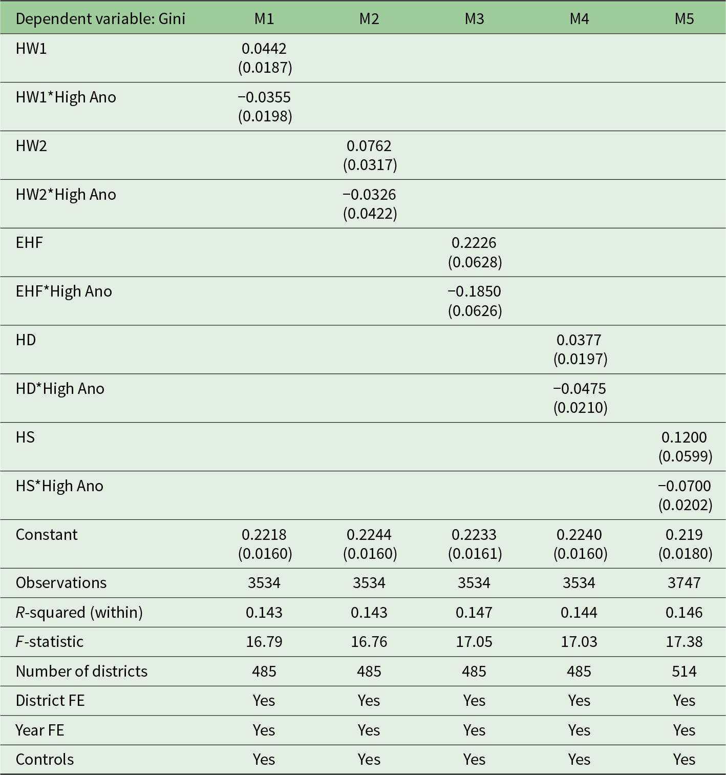
Extreme heat has worsened the skewed distribution of consumption expenditure in India. The net impact of heat on inequality depends on the extent of adaptability to extreme heat. The interaction term between the EHF and the temperature anomaly has a negative and statistically significant coefficient (Table 2). The negative sign shows that high-temperature anomalies reduce the impact of heatwaves on inequality. This finding indicates adaptation to heatwaves when they are accompanied by high-temperature anomalies (Models 1–4). For heat stress (Model 5), the interaction coefficient between heat stress and temperature anomaly is negative, indicating adaptation to heat stress under high-temperature anomalies.
6.3. Adaptation
The first indication of adaptation appears in Table 2, where the coefficient of the temperature anomaly is negative when the temperature anomaly interacts with extreme heat. The interaction term (Table 2) suggests that the negative association between extreme heat and inequality weakens at higher temperature anomaly levels, indicating adaptation to extreme heat. However, not all districts have the same level of temperature anomaly and adaptability. Therefore, the districts are categorised as low- and high-temperature anomaly districts.
The heatwave has increased consumption inequality in the study period (Table 2). A similar effect is observed when the temperature anomaly is low (Table 3). In districts with low anomalies, people are more sensitive to heatwaves and have low adaptability; therefore, extreme heat in such districts exacerbates consumption disparities. The interaction terms of extreme heat and the high anomaly are negative. This indicates that high-anomaly districts moderate the effect of heat on consumption distribution. The results suggest that the vulnerable section of society living in high-temperature anomaly districts is adapting to extreme heat. The results align with previous studies: hotter districts in India that use inter- and intra-crop adaptation are adapting to heat (Taraz, Reference Taraz2018).
Adaptation to extreme heat (fixed-effects regression)
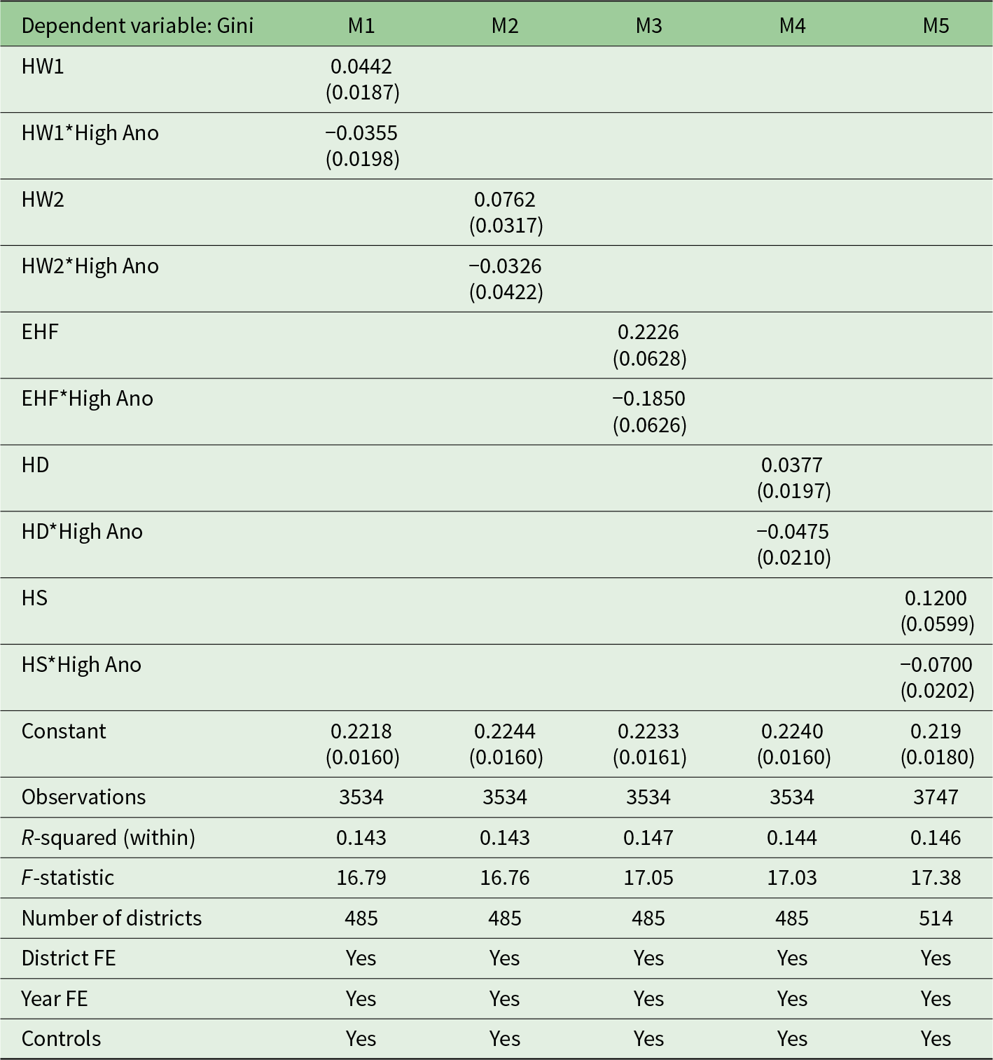
Table 3 Long description
The table reports fixed-effects regression results with the Gini index as the outcome across five model specifications, each using a different extreme-heat measure and its interaction with high temperature anomaly. In model 1, HW1 is associated with an increase in Gini (0.0442), while the HW1 interaction with high anomaly is negative (−0.0355), indicating a reduced effect in high temperature anomaly areas. Other measure of extreme heat also shows similar results. Model 5 shows HS is positive (0.1200) with a negative interaction (−0.0700), again indicating adaptation in high temperature anomaly districts . All models include district and year fixed effects and controls; standard errors are clustered at the district level.
Source: Authors’ calculations.
Note: District-level clustered standard errors in parentheses.
6.4. Agricultural channel
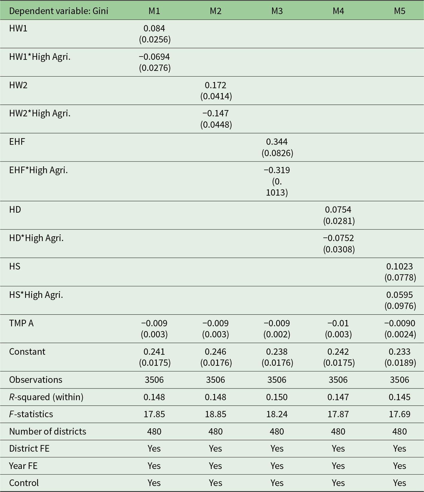
Based on the conceptual framework and prior literature, one observation is that agriculture is a vital channel through which extreme heat affects the distribution of consumption expenditure. From an aggregate perspective, heatwaves increase inequality in India (Tables 2 and 3). Heat affects poverty and inequality largely through the agricultural sector (Hallegatte et al., Reference Hallegatte, Bangalore, Bonzanigo, Fay, Kane, Narloch, Rozenberg, Treguer and Vogt-Schilb2016). Accordingly, the impacts of extreme heat on inequality are likely to vary between districts with low and high agricultural intensity, reflecting differences in adaptation capability. We categorise the districts by agricultural intensity. Table 4 examines the agricultural channel through which extreme heat and inequality are linked. The coefficient of interaction between heatwaves and high-agricultural-intensity districts is negative, indicating that, when high-agricultural-intensity districts are included, the impact of heatwaves on inequality diminishes. The coefficient for low-agricultural-intensity districts, or more urban-intensity districts, is positive, indicating an adverse impact on consumption distribution and no sign of adaptation.
Agricultural intensity, extreme heat and inequality (fixed-effects regression)
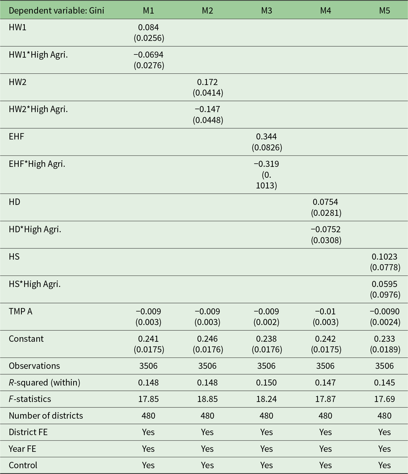
Table 4 Long description
The table reports five fixed-effects regressions with the Gini coefficient as the outcome and different extreme-heat measures as the explanatory variable, each interacted with an indicator for high agricultural intensity. In model 1, HW1 increases inequality, the coefficient is 0.084, while the HW1 interaction with high agriculture is negative (-0.0694), implying that districts with higher agricultural intensity are adapting to extreme heat. Similar results are found when other indices for extreme heat are considered in models 2, 3, and 4. In model 2, HW2 is positive (0.172) and its high-agriculture interaction is negative (-0.147), In model 3, EHF is strongly positive (0.344) with a negative high-agriculture interaction (-0.319), In model 4, HD is positive (0.0754) and the high-agriculture interaction is nearly equal in magnitude and negative (-0.0752). Model 5 differs: HS is positive (0.1023) and its interaction with high agriculture is also positive (0.0595). Each model uses 3,506 observations and 480 districts. With district and year fixed effects and additional controls are used; within R-squared values are about 0.145 to 0.150.
Source: Authors’ calculations.
Note: District-level clustered standard errors in parentheses.
To minimise climate-related risks in agricultural production, the government has introduced missions and policies, such as the National Mission for Sustainable Agriculture, which focuses on addressing challenges related to sustainable farming and on effective adaptation measures to overcome the threat of food insecurity and enhance livelihood opportunities (Gupta and Pathak, Reference Gupta and Pathak2016). Farmers are already adapting inter- and intra-crop strategies to limit the consequences of extreme heat on crops and yields (Taraz, Reference Taraz2018). Districts with low agricultural intensity can also be characterised by a relatively high share of the industry and services sector. In highly industrialised districts, low-income workers frequently engage in heat-exposed occupations, including construction activities. These workers have a lower capacity for adaptation to extreme heat. Their income and consumption might decrease due to reduced productivity when working in high temperatures (Kjellstrom et al., Reference Kjellstrom, Holmer and Lemke2009; Somanathan et al., Reference Somanathan, Somanathan, Sudarshan and Tewari2021).
7. Robustness check
Using the fixed-effects model, we employed a range of extreme heat measures, and the results are robust. We clustered the standard error at the district level in the main model. For robustness, the study uses the Conley standard error with 50- and 100-km distance cut-offs (see Supplementary Appendix Tables A9 and A10). Our results do not rely on the Gini coefficient alone; they remain robust when generalised entropy and the Atkinson index, with varying sensitivity values, are included in the regression as inequality indices (see Supplementary Appendix Tables A11–A15). We assessed robustness using alternative measures of precipitation: precipitation anomaly, the mean SPI index and a dummy variable derived from SPI. Altering the control for precipitation does not change our main findings (see Supplementary Appendix Tables A16–A18).
7.1. Dynamic panel regression model
The previous year's inequality may influence the current year's inequality. Therefore, the study considers a dynamic panel regression model that includes the lagged Gini as a regressor. The lagged Gini has a statistically positive impact on the current level of inequality (Supplementary Appendix Table A19). The results are robust, showing an increase in heatwaves, hot days and heat stress, widening the inequality. The results are also robust with respect to the adaptation channel. Negative signs of interactions between extreme heat (heatwaves, hot days, heat stress) and temperature anomalies indicate adaptation in districts with higher temperature anomalies. The results are consistent across fixed-effects and dynamic panel models. An increase in the proportion of extreme heat in a year widens the distribution of consumption expenditure in India. We conduct the Arellano–Bond test for serial correlation and find no evidence of second-order serial correlation (AR (2)) in the idiosyncratic disturbance term (see Supplementary Appendix Table A20). Further, instrument exogeneity is a key requirement for the consistency of GMM estimators. We perform the Sargan and Hansen test. The over-identification test fails to reject the null of instrument validity, supporting the appropriateness of the instruments for GMM estimation (see Supplementary Appendix Table A21).
7.2. DML
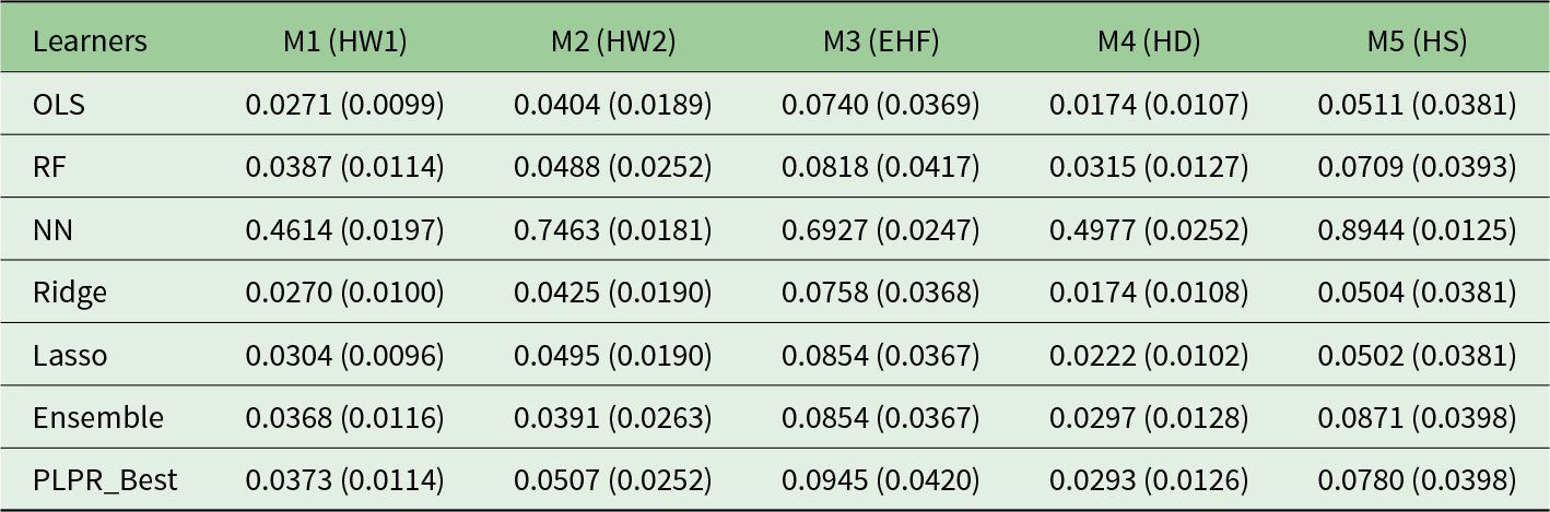
Table 5 reports the causal effects of heatwaves (HW1, HW2 and EHF), hot days and heat stress on inequality after partialling out the effects of cofounders. Row (1) is estimated using OLS, whereas the subsequent columns present DML results based on alternative learners. We found a positive and statistically significant causal effect of excessive heat on inequality. Heatwaves, hot days and heat stress contribute to the widening of inequality (Table 5).
Causal effect of extreme heat on inequality
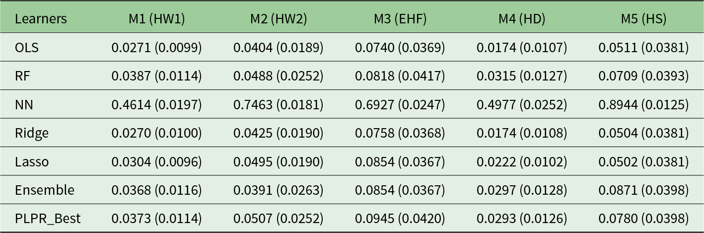
Table 5 Long description
The table reports estimated causal effects of extreme heat on an inequality outcome across five heat measures (HW1, HW2, EHF, HD, HS) using the double machine learning. Random Forest, Neural Network, Ridge and Lasso are different machine learning learners presented in the table. Then the ensemble and best model results are presented. All the coefficients are positive, illustrating that extreme heat increases the inequality. Neural Network produces much larger estimates than the other methods for every heat measure, ranging from about 0.46 (HW1) to about 0.89 (HS), with relatively small reported uncertainty. OLS, Ridge, and Lasso are similar and small, generally around 0.02 to 0.09 across measures; for example OLS is about 0.03 for HW1 and about 0.07 for EHF. Random Forest and the Ensemble are modestly higher than OLS-type models, such as Random Forest at about 0.08 for EHF and about 0.07 for HS. PLPR_Best is among the larger non-neural estimates, reaching about 0.09 for EHF and about 0.08 for HS. Across most non-neural methods, EHF and HS tend to yield the larger effects compared with HW1 and HD. Standard errors are clustered at the district level.
Notes: RF: Random Forest; NN: Neural Network. District-level clustered standard errors in parentheses.
Source: Authors’ calculations.
8. Conclusion and policy implications
Economic outcomes are adversely affected by climate change through multiple direct and indirect pathways. Existing studies have extensively examined the effects of climate change on economic outcomes, cross-country income distribution and human health. However, the impact of climate change varies with local geographic features, climatic conditions, the proportion of vulnerable people, adaptability and mitigation strategies within countries. Therefore, understanding how extreme heat affects inequality requires country-specific investigation. This study examines the effect of extreme heat on inequality at the district level in India from 2014 to 2022. The presence of substantial district-level disparities underscores the need for district-level climate change mitigation policies, alongside central and state interventions.
Our findings show that an increase in heatwaves within a year exacerbates the skewed distribution of consumption expenditure in India during the study period. Even considering the hot day, which is calculated based on a 1-day window, has an impact that increases the inequality. Immediate action is needed because extreme heat has a disproportionately negative impact on vulnerable segments of society. Poor people are suffering more from an increase in the number of heatwaves and hot days. Further, we examined the impact of heat stress on inequality. We found that heat stress has adverse distributional effects on consumption. Working in an environment with extreme heat reduces workers’ productivity. The economically disadvantaged are at greater risk of extreme heat because they are more likely to work in heat-exposed sectors, including construction and agriculture. Therefore, there is a need for a comprehensive policy framework and adaptation measures to address the extreme heat-induced inequality. Physically intensive work requires structured rest periods to safeguard workers’ health and safety. Measures such as scheduled water breaks, shaded rest periods and self-pacing are effective in reducing the adverse effects of heat stress on health and productivity. However, their implementation is often limited by employers’ concerns that additional breaks reduce productivity. Failing to adopt such measures increases the risk of presenteeism, absenteeism and higher medical expenditures, ultimately imposing greater economic costs on both workers and employers. Strengthening workplace heat-mitigation guidelines and enforcement can therefore improve labour productivity while reducing health-related costs.
The way extreme heat alters the distribution of consumption expenditure is complex, as outlined in the conceptual framework. The study explores the channels through which excessive heat affects inequality, with a focus on adaptability. We categorised the districts as low- or high-temperature anomaly districts and found that districts with high-temperature anomalies are adapting to extreme heat, whereas districts with low-temperature anomalies are not. Therefore, the categorisation of districts into high- and low-temperature anomaly groups is essential for designing targeted heat-mitigation policies.
As agriculture is a vital channel through which extreme heat affects inequality, we examined the varying effects of excessive heat on inequality between high and low agriculturally intensive districts. Public investment should support the adoption of farm mechanisation and climate-smart technologies to reduce reliance on manual labour in heat-exposed agricultural activities, thereby lowering farmers’ and agricultural labourers’ direct exposure to extreme heat. We found that people living in high-agricultural-intensity districts tend to adapt to extreme heat, whereas those in low-agricultural-intensity districts exhibit limited adaptive responses. Therefore, further classification of districts into high and low agriculturally intensive districts is crucial for effective policy formulation to reduce the adverse effects of extreme heat.
Strategies intended to manage extreme heat, such as access to hydration, rest scheduling, shade and sanitation, should be embedded within broader labour policies that improve work organisation, including flexible hours, greater job autonomy and stronger social protection mechanisms, to safeguard worker health and productivity in extreme heat.
Supplementary material
The supplementary material for this article can be found at https://doi.org/10.1017/S1355770X2610062X.
Data availability statement
We do not have permission to share the CMIE data used in this study, as it is paid. However, all other data used in the study are publicly available and can be accessed through their respective sources.
Acknowledgements
We thank the Co-Editor, S. Ferreira, the Associate Editor and the anonymous referees for helpful comments and suggestions. We sincerely thank Dr Elena Paglialunga for her guidance in calculating the heatwave indices. We are also grateful to the audience and panel of the conference, 2nd Edition of The Political Economy of Ecological Change and Economic Security in the Global South, held at the Centre for South Asian Studies, University of Cambridge, for their insightful comments and suggestions.
Funding statement
There is no source of funding.
Competing interests
The authors declare that they have no financial or non-financial competing interests directly or indirectly related to the work submitted for publication.