


1. Introduction
Compressible turbulent round jets have been widely studied for many years as they commonly occur at the exit of turbojet engines. It is known that compressibility significantly affects the jet spreading rate. Reduction of the jet spreading rate due to compressibility was observed in simulations and experiments. The reduction in spreading rate of compressible shear layers with increasing Mach number has been reported in the literature and related to the Reynolds shear stress and pressure–strain correlations. The effects of compressibility on the entrainment in jets have not been widely studied although they are of great interest.
In studies of interfaces in free shear flows, the flow is usually split into two regions. The region with high vorticity levels is the turbulent (T) region, whereas the other region which is largely irrotational is the non-turbulent (NT) region. The process of entrainment takes place in a thin region of finite thickness between the two, known as the turbulent/non-turbulent (T/NT) interface. The thickness of this layer has been stated to be of the order of the Taylor microscale. This layer has been further divided into a viscous superlayer whose thickness is of the order of the Kolmogorov microscale and a turbulent sublayer whose thickness is of the order of the Taylor microscale (da Silva & Pereira Reference da Silva and Pereira2008; da Silva et al. Reference da Silva, Hunt, Eames and Westerweel2014).
There have been several studies where the invariants of the velocity gradient tensor (VGT) have been studied for compressible flows. Foysi, Sarkar & Friedrich (Reference Foysi, Sarkar and Friedrich2005) performed VGT analysis of direct numerical simulation (DNS) data of compressible isotropic turbulence at various turbulent Mach numbers. Suman & Girimaji (Reference Suman and Girimaji2010) performed VGT analysis of compressible isotropic turbulence and showed the influence of dilatation levels on the flow topology. Wang & Lu (Reference Wang and Lu2012) studied the invariants in supersonic boundary layers while Kumari et al. (Reference Kumari, Mahapatra, Ghosh and Mathew2018) performed VGT analysis for supersonic pipe, nozzle and diffuser flows. In the last three studies mentioned above, it was found that the flow regions with expansion have unstable topologies and those with compression have stable topologies.
DNS of an incompressible, temporal round jet by Mathew & Basu (Reference Mathew and Basu2002) has shown that the total amount of fluid entrained by small scale motions at the interface is significant and the entrainment which happens around the Kolmogorov microscales is dominant.
DNS of an incompressible, temporal plane jet was performed by da Silva & Pereira (Reference da Silva and Pereira2008) to study the invariants of velocity gradient, rate-of-strain and rate-of-rotation tensors based on DNS data. They observed that the classical ‘teardrop’ shape of the joint probability density function (p.d.f.) of  $Q$ and
 $R$ (second and third invariants of the VGT) which is a feature of the turbulent region is absent at the T/NT interface.
Mathew, Ghosh & Friedrich (Reference Mathew, Ghosh and Friedrich2016) studied the behaviour of invariants of the VGT at the T/NT interface in compressible plane, temporal mixing layers based on DNS data. They observed a new flow topology i.e. the presence of tube-like structures at the T/NT interface at high Mach numbers which was not observed at lower Mach numbers.
In their study of inert and reacting temporal compressible mixing layers based on DNS, Mathew, Mahle & Friedrich (Reference Mathew, Mahle and Friedrich2008), calculated the change to fractal dimension of the T/NT interface and found it to fall with increasing convective Mach number, consistent with a reduction in interface surface area.
Nagata, Watanabe & Nagata (Reference Nagata, Watanabe and Nagata2018) studied temporally evolving compressible planar jets at Mach numbers of 0.6, 1.6 and 2.6. They observed that the thicknesses of the T/NT layer, viscous superlayer and the turbulent sublayer scale with the Kolmogorov microscale and also that the thickness at the turbulent sublayer reduces as the Mach number increases. They observed sharp changes in conditionally averaged thermodynamic quantities across the interface. They also studied the effect of compressibility on entrainment and observed that the surface area of the T/NT interface per unit area of the plane perpendicular to the cross-stream direction decreases as the Mach number increases, leading to a reduction in entrainment.
Motivated by the observation of a new flow topology at the T/NT interface in compressible mixing layers, we look for a similar feature in compressible round jets. In particular, it is of interest to know in which regions of the jet this new topology appears and to what extent. In the present work, we carry out DNS of a round jet at a Mach number of 0.9 and Reynolds number of 3600 at the inflow and study the invariants of the velocity gradient and rate-of-strain tensors in different regions along the jet in order to gain more insights into the local flow topology. In the present spatially evolving jet, the local centreline Mach number decays substantially in the axial direction to low subsonic values and it is to be seen in what way the flow topology found in the compressible region of the jet follows this Mach number change and changes towards the topology found in incompressible flows. Such a study is not found in the literature, since the convective Mach number was constant (in the streamwise direction) in the previous study of topology in compressible temporal mixing layers (Mathew et al. Reference Mathew, Ghosh and Friedrich2016).
2. Methodology
2.1. Governing equations, discretization methods, flow and computational parameters
The governing equations for compressible flow (Ghosh, Foysi & Friedrich Reference Ghosh, Foysi and Friedrich2010) are expressed in a characteristic form in generalized curvilinear coordinates (Sesterhenn Reference Sesterhenn2000) involving the primitive variables pressure (p), velocity (u) and entropy (s) as given below
 \begin{gather} p_t = \frac{\rho c}{2}[X^+{+} X^-{+} Y^+{+} Y^-{+} Z^+{+} Z^-] + \frac{p}{C_v}[s_t + X^s + Y^s + Z^s], \end{gather}
 \begin{gather}u_t ={-} \frac{\sqrt{g^{11}}}{2}[X^+{+} X^-] - Y^u - Z^u + \frac{\xi_{,i}^1 \xi_{,j}^l}{\rho}\frac{\partial \tau_{ij}}{\partial \xi^l} , \end{gather}
 \begin{gather}v_t ={-} \frac{\sqrt{g^{22}}}{2}[Y^+{+} Y^-] - X^v - Z^v + \frac{\xi_{,i}^2 \xi_{,j}^l}{\rho}\frac{\partial \tau_{ij}}{\partial \xi^l} , \end{gather}
 \begin{gather}w_t ={-} \frac{\sqrt{g^{33}}}{2}[Z^+{+} Z^-] - X^w - Y^w + \frac{\xi_{,i}^3 \xi_{,j}^l}{\rho}\frac{\partial \tau_{ij}}{\partial \xi^l} \end{gather}
 \begin{gather}s_t ={-}X^s - Y^s - Z^s + \frac{1}{\rho T}\left(-\xi_i^l\frac{\partial}{\partial \xi^l}\left(-\lambda\xi_i^l \frac{\partial T}{\partial \xi^l}\right) + \varPsi\right). \end{gather}
These equations are solved along with the ideal gas equation  $p = \rho RT$ (
 $\rho$ is the density), with constant
 $C_p$,
 $C_v$ (specific heats at constant pressure and volume respectively) and Prandtl number (
 $Pr = 0.71$). The dynamic viscosity is assumed to vary with temperature according to the power law:
 $\mu \propto T^{0.7}$. Bulk viscosity effects are neglected. Here,
 $X^{\pm },Y^{\pm },Z^{\pm }$ can be interpreted as acoustic waves propagating with velocities
 $u {\pm } \sqrt {g^{11}}c$,
 $v {\pm } \sqrt {g^{22}}c$ and
 $w {\pm }\sqrt {g^{33}}c$.
 $X^s,Y^s,Z^s$ are entropy waves propagating with velocities
 $u,v$ and
 $w$; and
 $X^{v,w}, Y^{u,w}, Z^{u,v}$ are vorticity waves traveling with velocities
 $u,v$ and
 $w$, according to the superscript as given below (c is the speed of sound)
 \begin{gather} X^{{\pm}} \equiv \left(u \pm \sqrt{g^{11}c}\right)\left[\frac{p_\xi}{\rho c} \pm \frac{u_\xi}{\sqrt{g^{11}}}\right], \end{gather}
 \begin{gather}X^{s} \equiv us_\xi , \end{gather}
 \begin{gather}X^{v} \equiv uv_\xi , \end{gather}
 \begin{gather}X^{w} \equiv uw_\xi. \end{gather}
The viscous stress tensor and the dissipation rate are given as follows:
 \begin{gather} \tau_{ij} = 2\mu(s_{ij} - \tfrac{1}{3}s_{kk}\delta_{ij}), \end{gather}
 \begin{gather} s_{ij} = \frac{1}{2}\left(\frac{\partial u_i}{\partial x_j} + \frac{\partial u_j}{\partial x_i}\right), \end{gather}
 \begin{gather} \varPsi = \tau_{ij}s_{ij}, \end{gather}
where  $g^{lm} = \xi _{,i}^l\xi _{,i}^m$ and
 $\xi _{,i}^l$ denote
 ${\partial \xi ^l}/{\partial x_i}$ such that
 ${\partial }/{\partial x_i} = ({\partial \xi ^l}/{\partial x_i}) ({\partial }/{\partial \xi ^l})$, where
 $x_i$ are Cartesian coordinates and
 $\xi^l$ are the computational space coordinates. The governing equations are solved using a fifth-order compact upwind scheme (Adams & Shariff Reference Adams and Shariff1992) for the convective terms and a sixth-order central scheme (Lele Reference Lele1992) for the molecular terms. Time integration is carried out using a low-storage third-order Runge–Kutta scheme (Williamson Reference Williamson1980). This formulation has been extensively used for DNS of supersonic pipe flow in cylindrical coordinates (Ghosh et al. Reference Ghosh, Foysi and Friedrich2010) and supersonic nozzle and diffuser flows in generalized curvilinear coordinates (Ghosh & Friedrich Reference Ghosh and Friedrich2014).
The governing equations are solved in cylindrical coordinates for the present study. The method given by Mohseni & Colonius (Reference Mohseni and Colonius2000) is used for axis singularity treatment. The domain size used is  ${{40r_0}} \times 10{{r_0}}$ in the axial (x) and radial (r) directions, respectively, where
 ${{r_0}}$ is the jet radius at inflow. The number of grid points employed are
 $800 \times 160 \times 250$ (
 $= 32 \times 10^6$) in the axial, azimuthal and radial directions, respectively. The grid spacing is uniform in the axial and azimuthal directions. The grid is stretched in the radial direction using the
 $sinh$ function. The grid has a minimum radial spacing of
 $\Delta r / r_{0} = 0.018$ (which is the same as that of Freund Reference Freund2001) at the jet centreline. In the axial direction we use uniform grid spacing of
 $\Delta x /r_{0} = 0.05$, which is the same as the minimum grid spacing used by Freund (Reference Freund2001). Thus, we maintain their minimum grid spacing, but in the present study, the grid spacing is kept uniform in the axial direction. With the abovementioned resolution, the present DNS, to the best of authors’ knowledge, is the best resolved DNS study of a round jet at the Mach and Reynolds numbers considered. The axial velocity spectrum in the azimuthal direction is shown in figure 1, at
 $r = r_0$ and
 $X / r_0 = 12$, 16 and 20. Jet centreline velocity at inflow (
 $u_0$) and jet radius (
 $r_0$) are used for normalizing the spectrum. The spectrum shows a proper decay over several decades and hence demonstrates that the present DNS resolution is adequate. The boundary conditions are explained in following subsection.
Axial velocity spectrum in the azimuthal direction at  $r = r_0$ and
 $X / r_0 = 12,16$ and 20, normalized using the centreline velocity at inflow (
 $u_0$) and the jet radius (
 $r_0$).

2.2. Boundary conditions
The axial velocity profile at inflow is specified as given in (2.13). This profile is the same as that of Freund (Reference Freund2001). A very weak coflow ( $u_{cof}$ in (2.13)) at Mach number
 $M_{\infty } = 0.009$ is imposed at the inlet beyond
 $r = r_0$, to ensure proper flow entrainment. The remaining two velocity components are set to zero at inflow. The vortex inflow-forcing method of Bogey, Bailly & Juvé (Reference Bogey, Bailly and Juvé2003) is used here, which is a rational way to disturb the initially laminar shear layer so that transition to turbulence occurs. The maximum value of the fluctuations added at inflow is 1% of the mean value. The temperature at the inflow is
 $255.59$ K. These values of
 $u, v, w$ and
 $T$ at the inflow are applied using the method discussed in Lodato, Domingo & Vervisch (Reference Lodato, Domingo and Vervisch2008). In this method, the incoming characteristics are calculated using the ‘expected’ values of the primitive variables at the inflow ((2.14)–(2.17)). Small variations in the primitive variables are allowed, so that the acoustic waves can leave the computational domain. In (2.14)–(2.18), the subscript
 $ex$ stands for the ‘expected’ (or target) value of a particular variable at the inflow boundary. The expected value of entropy at inflow is found using the values of temperature and density at inflow. The expected values of the flow variables are kept constant during the simulations. The parameters
 $\eta _{1}, \eta _{2}, \eta _{3}$ and
 $\eta _{4}$ are constants, whose values depend on the particular flow case. In the present study
 $\eta _{1} = \eta _{2} = \eta _{3} = \eta _{4} = 3.58$. The parameters
 $X^+, X^{v}, X^{w}$ and
 $X^{s}$ are the incoming characteristics at inflow (Sesterhenn Reference Sesterhenn2000). Pressure and density at inflow are uniform, except for the changes that occur due to soft boundary conditions. The transverse terms of the governing equations at the inflow are set to zero (as suggested in Lodato et al. Reference Lodato, Domingo and Vervisch2008)
 \begin{gather} u= \frac{u_{0}}{2} \left[ 1 - \tanh \left\{ 12.5 \left(\frac{r}{r_{0}} - \frac{r_{0}}{r}\right) \right\} \right] + u_{cof}, \end{gather}
 \begin{gather}X^+{=} \eta_{1}\frac{\rho c^2 (1-M^2)}{L_x}(u-u_{ex}), \end{gather}
 \begin{gather}X^v = \eta_{2}\frac{c}{L_x}(v-v_{ex}), \end{gather}
 \begin{gather}X^{w} = \eta_{3}\frac{c}{L_x}(w-w_{ex}), \end{gather}
 \begin{gather}X^{s} = \eta_{4}\frac{c}{L_x}(s-s_{ex}). \end{gather}
A partially non-reflecting boundary condition (Poinsot & Lele Reference Poinsot and Lele1996) is applied at the radial outflow boundary. Near the outflow in the axial direction, a sponge layer is specified. The outflow sponge used is similar to that used by Sandberg, Sandham & Suponitsky (Reference Sandberg, Sandham and Suponitsky2012). The incoming characteristic ( $\mathcal {L}$) is gradually set to a partially non-reflecting boundary condition in the sponge zone, as shown in (2.18). The sponge layer at the outflow starts at
 $x_{s} = x/r_0 = 35$ and ends at
 $x_{f} = x/r_0$ = 40. In (2.18), the value of constant
 $\sigma$ depends on particular flow cases
 \begin{gather} \mathcal{L} = \mathcal{L}g(x) + (1-g(x)) \sigma (p-p_{ex}), \end{gather}
 \begin{gather} g(x) = 0.5 \left\{1 + \cos\left[\frac{{\rm \pi}(x-x_{s})}{(x_{f}-x_{s})} \right] \right\}. \end{gather}
The current study is focused on an isothermal round jet at a Mach number of 0.9 and Reynolds number of 3600 based on the jet diameter and jet centreline velocity at inflow. The flow parameters of present study and the reference results used for comparison are summarized in table 1. The results obtained from the DNS are shown in the following section.
Flow parameters.

3. Results and discussion
Before discussing the main results of this paper – the VGT analyses – some results from the DNS are shown briefly, comprising instantaneous fields, mean flow and turbulence statistics, to establish the correctness of the present simulations and to validate with the existing literature. Hence, the results are organized as follows: first, the instantaneous results are shown, followed by the mean flow results and turbulence statistics. Finally, the results from the VGT analysis are presented.
3.1. Comparison of DNS results with reference studies
3.1.1. Instantaneous flow field
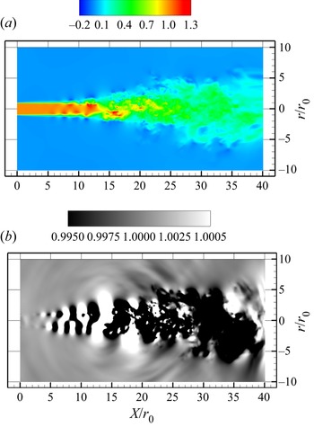
The instantaneous axial velocity and pressure are shown in figure 2 where the potential core of the jet is clearly visible. After the end of the potential core, the spreading of the jet in the radial direction and a reduction in the centreline axial velocity can be observed. Large pressure fluctuations can be seen in the potential core region as the instabilities start to grow. No issues with boundary conditions and sponge layers are noticed in these plots.
Instantaneous (a) axial velocity (normalized using the centreline velocity at inflow ( $u_0$)) and (b) pressure (normalized using ambient pressure) plotted on an axial–radial plane.

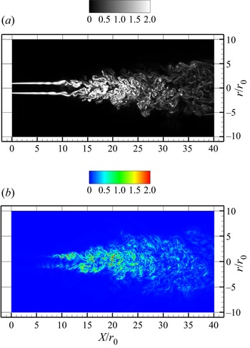
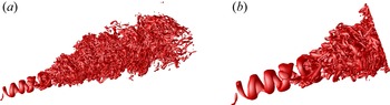
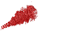
The instantaneous vorticity magnitude in an axial–radial plane is shown in figure 3(a). The distortion and merging of shear layers can be clearly seen in this figure. As can be seen in the figure, as we move in the downstream direction after the potential core, the jet starts spreading in the radial direction and the vorticity magnitude decreases. The instantaneous dilatation is shown in figure 3(b). As can be seen, the dilatation levels reduce as we move in the downstream direction as the Mach number decreases. We now show isosurfaces of positive Q in figure 4. The helical shape of the initial vortical structure can be seen in the potential core. As we move in the downstream direction, the instabilities grow and the flow subsequently becomes turbulent.
Instantaneous (a) vorticity magnitude and (b) dilatation (both normalized using the centreline velocity at inflow ( $u_0$) and the jet radius at inflow (
 $r_0$)) plotted on an axial–radial plane.

Isosurface of  $Q=0.1$ (normalized using jet centreline velocity and radius at inflow); (a)
 $X / r_0$ = 5 to 40 (b)
 $X / r_0$ = 5 to 20 (normalized using
 $u_0$ and
 $r_0$).

3.1.2. Mean flow results
We first look at mean flow quantities in the axial direction along the centreline plotted up to the beginning of the sponge region. The mean centreline axial velocity along the axial direction is shown in figure 5(a). The end of the potential core, followed by a decay of the centreline velocity, can be clearly seen. The results match closely with those of Freund (Reference Freund2001). The inverse of centreline velocity,  $u_0/u_{cl}(X)$, is shown in figure 5(b). The linear variation of
 $u_0/u_{cl}(X)$ can be seen after the end of the potential core. It is known from order-of-magnitude analysis and experiments that the centreline velocity,
 $u_{cl}(X)$, of round jets decays as
 \begin{equation} \frac{u_{cl}(X)}{u_{0}}= B_{u} \left[\frac{2r_{0}}{X - X_{0}} \right], \end{equation}
where  $X_{0}$ is the virtual origin and
 $B_{u}$ is an empirical constant which from experiments of high Reynolds number incompressible round jets is found to be around 6. In the present compressible case at low Reynolds number,
 $B_{u}$ = 5.67. Freund (Reference Freund2001) has shown that the linear fit with the value
 $B_{u}$ = 5.8 matches closely with his data.
(a) Centreline axial velocity, (b) inverse of centreline axial velocity and (c) centreline Mach number. Symbols in all panels are the results of Freund (Reference Freund2001).

The centreline Mach number variation is shown in figure 5(c) and we note that the Mach number drops below  $0.6$ after X = 20
 $r_0$. Here, also we note a very good agreement with the results of Freund (Reference Freund2001).
3.1.3. Reynolds stresses
The evolution of the axial Reynolds stress and Reynolds shear stress in the axial direction is shown in figure 6. The profiles are normalized using the jet centreline velocity at inflow ( $u_0$). The radial coordinate is normalized using the jet radius at inflow. As can be seen in figure 6, before the potential core ends near
 $X = 8$
 $r_0$, the stresses have small values. Then, they rise rapidly, reach the maximum values and then decrease. The peaks observed in the present study are higher compared with those of Freund (Reference Freund2001) at a couple of streamwise locations. Then, subsequently, the peaks are reduced and the profiles grow in the radial direction. Radial profiles of axial, radial and Reynolds shear stresses normalized using the local jet centreline velocity (
 $u_{cl}$) are shown in figure 7. The profiles are compared with those of Freund (Reference Freund2001), Picano et al. (Reference Picano and Casciola2007) and Panchapakesan & Lumley (Reference Panchapakesan and Lumley1993). The radial coordinate is normalized using the axial location. The axial Reynolds stress profile is shown in figure 7(a). The present profile is in agreement with the reference results away from the jet centreline. Near the jet centreline the profile is close to that of Picano et al. (Reference Picano and Casciola2007). The radial Reynolds stress and Reynolds shear stress profiles are also shown in figures 7(b) and 7(c), respectively. As can be seen in the figure, the present results are close to the reference results. Overall, good agreement is observed for all three components of the Reynolds stress.
Evolution of (a) the axial Reynolds stress and (b) Reynolds shear stress; solid line represents the present study, symbols are the results from Freund (Reference Freund2001) (normalized using the jet centreline velocity at inflow ( $u_0$)).

(a) Axial Reynolds stress, (b) radial Reynolds stress, (c) Reynolds shear stress (normalized using jet centreline velocity ( $u_{cl}$)), present study: ———, red
 $x / r_0 = 30$, Freund (Reference Freund2001):
 $\bullet$, red
 $x / r_0 = 30$; Picano et al. (Reference Picano and Casciola2007):
 $\bullet$, green, Panchapakesan & Lumley (Reference Panchapakesan and Lumley1993):
 $\bullet$, blue.

3.2. Velocity gradient tensor analysis
The VGT  $\boldsymbol {A}$, consisting of elements,
 $A_{ij} = {\partial u_{i}}/{\partial x_{j}}$, has three invariants:
 $P = -{\rm trace}(A), Q = \tfrac {1}{2}$ [
 $P^2 - {\rm trace}(A^2)$];
 $R = -{\rm det}(A)$. For incompressible flow
 $P = 0$,
 $P> 0$ where the fluid is being compressed and is negative in regions of expansion. Real values of the eigenvalues of
 $\boldsymbol {A}$ are found when the discriminant
 $D < 0$, where
 $D = 27$
 $R^2 + (4P^3 - 18PQ)R + ( 4Q^3 - P^2 Q^2)$. The parameter
 $\boldsymbol {A}$ can be split into symmetric strain-rate and skew–symmetric rotation-rate parts:
 $\boldsymbol {A} = \boldsymbol {S} + \boldsymbol {W}$. Using subscripts
 $S$ and
 $W$ to denote invariants of these two tensors,
 $P_{W} = R_{W} = 0$ for all flows;
 $P_{S} = P$,
 $Q_{S} = - \tfrac {1}{2}S_{ij}S_{ji}$,
 $R_{S} = - \tfrac {1}{2} S_{ij}S_{jk}S_{ki}$ and
 $Q_{W} = - \tfrac {1}{2} W_{ij}W_{ji}$ (see Chong, Perry & Cantwell Reference Chong, Perry and Cantwell1990 for details).
The joint p.d.f.s of invariants  $(Q,R)$ and (
 $Q_{S}, R_{S}$) are computed based on instantaneous VGT and by dividing the
 $3\sigma$ range (where
 $\sigma$ is the standard deviation) into 200 equispaced bins. The analysis was performed at different time instants after the jet has developed and the results are shown here for a particular time instant. The trends reported here have been observed at various time instants. In the analysis, we considered different sets of grid points to compute the joint p.d.f.: (i) all grid points in the domain segment, (ii) points in the T and NT regions separately and (iii) points at the boundary between these two regions and (iv) points in the interface between these two regions. In our study, the boundary is considered to be the surface defined by the points where the vorticity magnitude first exceeds a defined threshold value when approached from the free stream. In the present study, this threshold is chosen as 10 % of the maximum of the mean vorticity magnitude in the domain segment under consideration at the particular time instant. Mathew et al. (Reference Mathew, Ghosh and Friedrich2016) have used the maximum mean vorticity to determine the threshold in their compressible mixing layers. In the present work, the T/NT interface is defined as a region that consists of the T/NT boundary and one layer above and below the boundary in the radial direction. This interface can be thought of as the region where the T/NT boundary is likely to lie when the vorticity threshold is increased or decreased slightly. Hence, the results shown for the interface allow for consideration for the points which would fall on the T/NT boundary if the threshold were varied slightly. The elements of the VGT,
 $\boldsymbol {A}$ – and hence its invariants – are normalized using the maximum mean (spatial average at the particular time instant) vorticity magnitude for a particular domain segment. It may be noted that a similar normalization has been previously used by Mathew et al. (Reference Mathew, Ghosh and Friedrich2016).
For the present VGT analysis, the domain is divided into four parts, each of length  $5 r_0$ in the axial direction i.e.
 $X = 10$ to
 $15 r_0$, 15 to
 $20 r_0$, 20 to
 $25 r_0$ and 25 to
 $30 r_0$. Since the centreline Mach number drops below 0.6 after
 $X = 20 r_0$, we do not expect any significant compressibility effects on the flow topology in the jet region further downstream. The p.d.f. of
 $P$, normalized with the mean maximum vorticity magnitude for a particular segment at the given time instant, within the range of
 $\pm$3
 $\sigma _{P}$ (
 $\sigma _{P}$ being the standard deviation of
 $P$) is shown in figure 8 for the segments mentioned above. As can be seen in the figure, the larger
 $P$ values are absent from the distribution in the regions
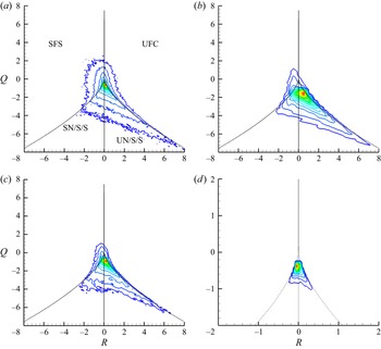
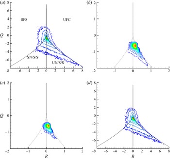
 $X / r_0 = 20$ to 25 and 25 to 30, where the p.d.f. becomes flatter as compared with the upstream locations. The absence of large dilatation values can also be observed in the instantaneous dilatation plot shown in figure 3(b). The joint p.d.f. of Q, R is shown in figure 9 for different segments of the domain, considering all points in a particular segment. The black solid lines in this and subsequent figures denote
 $PQ - R = 0$ (top line) and
 $D=0$ (bottom two lines) (refer to Suman & Girimaji Reference Suman and Girimaji2010). In the plots where the joint p.d.f.s are not conditioned on the sign of
 $P$, the above curves are shown for
 $P=0$ while the average (here the average is calculated using the instantaneous values of
 $P$ used for the conditioned plots) positive or negative values of
 $P$ are used to obtain the curves where the joint p.d.f.s conditioned on
 $P$ are shown. The different flow topologies detailed in Chong et al. (Reference Chong, Perry and Cantwell1990), appearing for positive and negative
 $P$ are marked in figure 13 and summarized in table 2. In all the joint p.d.f. plots, around 20 contour levels are plotted including the maximum and minimum values of the p.d.f. In figure 9(a) we mark the topologies for
 $P = 0$. As can be seen in figure 9(a), the developed region shows the classic teardrop shape observed in many studies. As we move upstream in the axial direction this shape keeps changing, as can be seen in figure 9(b,c). The shape is very different in figure 9(d) and we notice the occurrence of a third quadrant lobe. This inclination towards the third quadrant observed at the upstream locations between
 $X=10$
 $r_0$ and 15
 $r_0$ may represent the presence of local tube-like structures. These regions will be analysed more closely now. Results for each segment of the domain are presented separately below and the centreline Mach number of each domain segment is mentioned for reference. Since the downstream segments show the familiar teardrop shape, they are presented first, followed by the upstream segments showing the new topology.
(i) Segment
 $X = 25$ to $30 r_0$ ($M$ = 0.45 to 0.38)


Description of flow topology acronyms.

The p.d.f. of  $P$ in different domain segments, the centreline Mach number rages from 0.89 to 0.81, 0.81 to 0.57, 0.57 to 0.45 and 0.45 to 0.38 in the respective domain segments (upstream to downstream).

Joint p.d.f. of Q, R considering all points in (a)  $x = 25$ to
 $30 r_0$, (b)
 $x = 20$ to
 $25 r_0$, (c)
 $x = 15$ to
 $20r_0$, (d)
 $x = 10$ to
 $15r_0$.

The results for the segment  $X = 25$ to
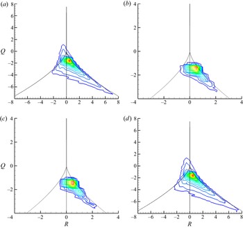
 $30 r_0$ are shown in figure 10. In this segment, the centreline Mach number ranges from 0.45 to 0.38. Results are shown considering all points (figure 10a), points in the NT region only (figure 10b), points in the T/NT boundary (figure 10c) and points in the turbulent region only (figure 10d). The p.d.f. shape looks very similar for figure 10(a,d) since in this segment of the domain, the flow is largely turbulent. The contours in figure 10(b,c) show an inclination towards the fourth quadrant where unstable topologies such as unstable node/saddle/saddle (UN/S/S) and unstable focus compressing (UFC) are present. This points towards the presence of sheet-like structures.
(ii) Segment
$X = 20$ to $25 r_0$ ($M$ = 0.57 to 0.45)


Joint p.d.f. of Q,R in the region  $X = 25$ to
 $30 r_0$; (a) all points, (b) NT region, (c) T/NT boundary, (d) T region.

The results for segment  $X = 20$ to
 $25 r_0$ are shown next in figure 11. In this segment, the centreline Mach number ranges from 0.57 to 0.45. Similar observation can be made for this segment of the domain as in the segment
 $X = 20$ to
 $25 r_0$, i.e. most of the region in the segment consists of turbulent flow. Also the p.d.f. shape in figure 11(b,c) shows the preference for sheet-like structures (UN/S/S and UFC topologies), similar to what was observed for the segment
 $X = 25$ to
 $30 r_0$.
Joint p.d.f. of Q,R in the region  $X = 20$ to
 $25 r_0$; (a) all points, (b) NT region, (c) T/NT boundary, (d) T region.

It may be noted here that in the region  $X = 20$ to
 $30 r_0$, the centreline Mach number is low and hence we do not expect substantial compressibility effects on the flow topology here. However, local dilatation may have some effects (which, it may be noted, are not compressibility effects in this low Mach number region) on the topology here. However, our analysis shows that the sign of dilatation has no effect on the flow topology in this region.
(iii) Segment
$X = 15$ to $20r_0$ ($M$ = 0.81 to 0.57)


The results for the domain segment  $X = 15$ to
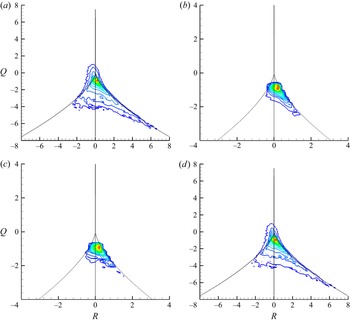
 $20 r_0$ are shown in figure 12. In this segment, the centreline Mach number ranges from 0.81 to 0.57. As can be seen in figure 12(b) the tail of the p.d.f. is oriented towards the fourth quadrant which represents preference for presence of sheet-like structures (UN/S/S and UFC topologies). A similar behaviour can also be seen in figure 12(c). Hence, we can say that it appears to be a feature of the T/NT boundary in this part of the domain. However, the sign of dilatation has a role to play, as will be shown now.
Joint p.d.f. of Q,R in the region  $X = 15$ to
 $20 r_0$; (a) all points, (b) NT region, (c) T/NT boundary, (d) T region.

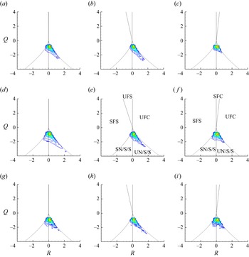
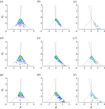
The effect of the sign of  $P$ on the joint p.d.f. is now shown in figure 13. The p.d.f. shapes are shown for the NT region, the T/NT interface and the T/NT boundary. As can be seen in the figure, the orientation of the p.d.f. shape towards the fourth quadrant (unstable topology UN/S/S) is the contribution of
 $P <$ 0 points. This orientation towards the fourth quadrant is not observed for
 $P > 0$ points, which points to a different flow topology in regions of compression. Here, we see the emergence of a third quadrant lobe indicating the presence of stable topology stable node/saddle/saddle (SN/S/S), which will be shown to be more prominent in further upstream locations. This lobe is visible especially at the T/NT interface and boundary, which points to the presence of tube-like structures. As expected, the local expansion regions have a preference for sheet-like structures with unstable topology UN/S/S. This applies to all three regions namely the NT region, T/NT interface and T/NT boundary.
Joint p.d.f. of Q,R in the region  $X = 15$ to 20
 $r_0$; (a–c) NT region, (d–f) T/NT interface, (g–i) T/NT boundary; (a,d,g) all P values, (b,e,h) only
 $P < 0$ points, (c,f,i) only P > 0 points.

In figure 14, we show the effect of the magnitude and sign of P on the local flow topology. For  $P = 0.1$ (
 $\pm$0.05), a tendency towards SN/S/S topology is clearly visible. Higher positive values of P in this segment show a lot of scatter and no clear trend (not shown here). When
 $P = -0.1$, then the joint p.d.f. shape points to UN/S/S topology. Again for
 $P = -0.2$, UN/S/S topology is visible but also there is some scatter in the data.
(iv) Segment
$X = 10$ to $15 r_0$ ($M$ = 0.89 to 0.81)


Joint p.d.f. of Q,R in the region  $X = 15$ to 20
 $r_0$; (a–c) NT region, (d–f) T/NT interface, (g–i) T/NT boundary; (a,d,g)
 $P = 0.1$, (b,e,h)
 $P = -0.1$, (c,f,i)
 $P = -0.2$.

Next, we show the results for the segment  $X = 10$ to
 $15 r_0$ in figure 15. In this segment, the centreline Mach number ranges from 0.89 to 0.81. Unlike previously shown domain segments, here, the p.d.f. shape for all points (figure 15a) matches closely with that for the NT region (figure 15b). This is expected as this segment largely consists of the NT region.
Joint p.d.f. of Q,R in the region  $X = 10$ to
 $15 r_0$; (a) all points, (b) NT region, (c) T/NT boundary, (d) T region.

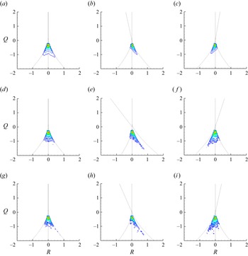
Now, in figure 16, we show the effect of the sign of  $P$ on the presence of tube-like structures. The p.d.f.s are shown for the NT region, the T/NT interface and the T/NT boundary. As can be seen in the figure, the p.d.f. shape is oriented towards the third quadrant for
 $P > 0$ points whereas it is oriented towards the fourth quadrant for
 $P < 0$ points. Hence, the compression regions have a preference for tube-like structures (with SN/S/S topology) in this portion of the jet. This applies to all three regions, namely, the NT region, the T/NT interface and the T/NT boundary.
Joint p.d.f. of Q,R in the region  $X = 10$ to
 $15 r_0$; (a–c) NT region, (d–f) T/NT interface, (g–i) T/NT boundary; (a,d,g) all
 $P$ values, (b,e,h) only
 $P < 0$ points, (c,f,i) only
 $P > 0$ points.

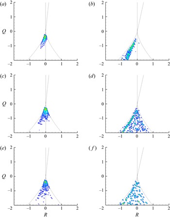
In figures 17 and 18, we show the effect of the magnitude and sign of  $P$ on the local flow topology. For
 $P = 0.1$ (
 $\pm$0.05), a tendency towards SN/S/S topology is clearly visible. For
 $P = 0.2$ (
 $\pm$0.05), a tendency towards SN/S/S topology is clearly visible in the NT region. At the T/NT interface and boundary, both SN/S/S and UN/S/S topologies appear. When
 $P = -0.025$ (lower negative
 $P$ value, figure 18), then the joint p.d.f. shape points to UN/S/S topology in the NT region. For the T/NT interface and boundary, SN/S/S topologies are also noticed, although the preference is towards UN/S/S topology. For
 $P = -0.1$, the tendency towards UN/S/S topology is clearly visible. This shows that the stable SN/S/S topology appears in the compression regions and also to some extent at the T/NT interface and boundary regions with weak expansion in this part of the jet.
Joint p.d.f. of Q,R in the region  $X = 10$ to
 $15 r_0$; (a,b) NT region, (c,d) T/NT interface, (e,f) T/NT boundary; (a,c,e)
 $P = 0.1$, (b,d,f)
 $P = 0.2$.

Joint p.d.f. of Q,R in the region  $X = 10$ to
 $15 r_0$; (a,b) NT region, (c,d) T/NT interface, (e,f) T/NT boundary; (a,c,e)
 $P = -0.025$, (b,d,f)
 $P = -0.1$.

This new topology, which appears prominently in this segment of the jet where the Mach number is high and the dilatation levels are also high, was first observed by Mathew et al. (Reference Mathew, Ghosh and Friedrich2016) for a plane, temporal mixing layer at convective Mach number of 1.1 which was not present at Mach number of 0.7. Similar observation regarding the effect of the sign of  $P$ on this third quadrant lobe was also made by Mathew et al. (Reference Mathew, Ghosh and Friedrich2016). They also observed this third quadrant lobe for small negative values of
 $P$, which disappeared at higher negative values of
 $P$. In the present round jet, a somewhat similar trend is seen in this particular segment. However, this aspect needs further investigation in jets at substantially higher Mach number which may be a focus of future studies.
3.3. Strain-rate tensor analysis
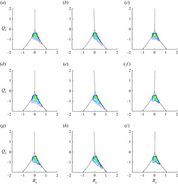
The invariants of the strain-rate tensor are also analysed for two segments of the domain. First, the results are shown for the segment  $X = 15$ to
 $20 r_0$ in figure 19. The results are shown for NT region, T/NT boundary and T/NT interface. As can be seen in the figure, the joint p.d.f. of
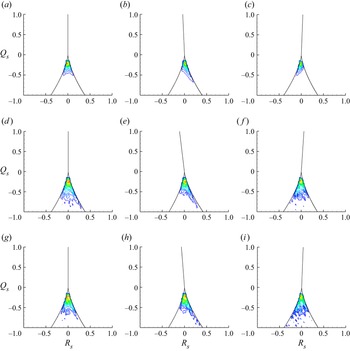
 $Q_s - R_s$ supports the observation made for the VGT. The orientation of the joint p.d.f. towards the fourth quadrant is a bit sharper for the strain-rate tensor.
Joint p.d.f. of invariants of strain-rate tensor between  $X = 15$ and
 $20 r_0$; (a–c) NT region, (d–f) T/NT interface, (g–i) T/NT boundary; (a,d,g) all
 $P$ values, (b,e,h) only
 $P <$ 0 points, (c,f,i) only
 $P > 0$ points.

The results for the segment  $X = 10$ to 15
 $r_0$ are shown in figure 20. Here also, the joint p.d.f. of
 $Q_s - R_s$ supports the observations made with the VGT, showing distinct third quadrant tails in regions with positive
 $P$.
Joint p.d.f. of invariants of strain-rate tensor between  $X = 10$ and
 $15 r_0$; (a–c) NT region, (d–f) T/NT interface, (g–i) T/NT boundary; (a,d,g) all
 $P$ values, (b,e,h) only
 $P <$ 0 points, (c,f,i) only
 $P > 0$ points.

4. Conclusions
Direct numerical simulation of a compressible round jet is performed at Mach number of 0.9 and Reynolds number of 3600. Instantaneous results are presented for velocity, pressure, dilatation and vorticity magnitude. The centreline velocity decay and the Reynolds stresses are shown and compared with the results of Freund (Reference Freund2001).
The VGT analysis of the flow is then carried out. To the best of authors’ knowledge, VGT analysis of a spatially developing compressible round jet is presented for the first time in the present study. The classic teardrop shape is observed in the joint p.d.f. of Q–R in the fully turbulent region of the jet. Between  $X = 15$ and
 $20 r_0$ where the centreline Mach number varies from 0.81 to 0.57, the joint p.d.f. contours are oriented towards the fourth quadrant when plotted for the NT region, the T/NT interface and the T/NT boundary. It is observed that this orientation towards the fourth quadrant, which denotes the presence of sheet-like structures (unstable topologies), is present when points with
 $P < 0$ are considered, but it is far less evident for the
 $P > 0$ points. For the points with
 $P > 0$, we observe a small third quadrant lobe. Between
 $X = 10$ and 15
 $r_0$, where the centreline Mach number varies from 0.89 to 0.81, the p.d.f. contours show some inclination towards the third quadrant when plotted for the NT region, the T/NT interface and the T/NT boundary. It is observed that this orientation towards the third quadrant, representing the presence of tube-like structures (stable topologies), is present when points with
 $P > 0$ are considered. These stable topologies also appear, to a lesser extent, in the regions with weak expansion but not in regions with relatively larger expansion. Such stable topologies are not found in the region after
 $X = 20 r_0$ where the Mach number is smaller than 0.6. Presence of this tube-like topology in the segment of the jet with relatively high subsonic Mach numbers and high dilatation levels, which was also observed by Mathew et al. (Reference Mathew, Ghosh and Friedrich2016) for compressible temporal mixing layers at high Mach numbers, may be a common feature at the T/NT interface region of compressible free shear layers. However, in the present study, the axial variation of the centreline Mach number leads to an interesting result. The present analysis indicates that changes to the VGT invariants and the implied changes to local topology do respond to the mean Mach number and the expected compressibility effects. This could not have been predicted from the previous study of compressible mixing layers where the Mach number was constant in the streamwise direction. The results, therefore, have consequences for changes to entrainment that differ from that in the plane, temporal mixing layers previously investigated. The strain-rate tensor analysis also shows similar trends as observed in the VGT analysis. In the present jet, the presence of the stable topologies occurs at normalized
 $P = 0.1$ and to a lesser extent for
 $P = 0.2$, and are seen clearly for positive
 $P$ in the region with high subsonic Mach number. These topologies are also observed (although to a much lesser extent) in this segment of the jet at the T/NT interface and boundary in regions with weak expansion. The appearance of stable topologies in regions of weak expansion was also observed in temporal compressible mixing layers by Mathew et al. (Reference Mathew, Ghosh and Friedrich2016). Further studies on jets at higher Mach number are needed to gain more insights into this aspect.
Acknowledgements
The computations were performed on the Paramshakti supercomputing facility at IIT Kharagpur.
Funding
The authors acknowledge the support of Science and Engineering Research Board (SERB), India through grant number CRG/2022/000377.
Declaration of interests
The authors report no conflict of interest.