



1. Introduction
Waves occur widely in real world phenomena. This includes waves in fluids, optics, acoustics and elasticity among many others. Linear waves find many important applications across various scientific disciplines. As such, their mathematical and physical properties have been extensively investigated dating back to the pioneers of dynamics. In comparison with their linear counterparts, nonlinear waves have been relatively less studied and, in certain cases, even their underlying processes are not so well understood. However, much more is known about weakly interacting nonlinear waves for which researchers often consider the dominant approximation to be a collection of Fourier modes.
In weakly nonlinear deep water waves, Stokes (Reference Stokes1847) found a relationship between the frequency and amplitude of the dominant Fourier mode. More than a hundred years later Benjamin & Feir (Reference Benjamin and Feir1967) showed that this wave was unstable. Soon afterwards, by allowing the envelope of the wave to vary slowly in space and time Zakharov (Reference Zakharov1968) (see also Zakharov Reference Zakharov1998) showed that the complex amplitude of the envelope satisfies a two space, one time dimensional nonlinear Schrödinger (NLS) equation. Remarkably, the one space and one time dimensional NLS equation was shown to be an integrable equation (Zakharov & Shabat Reference Zakharov and Shabat1972). The integrability of the NLS equation followed after another well-known one-dimensional equation, the Korteweg–de Vries (KdV) equation was found to be an integrable system (Gardner et al. Reference Gardner, Greene, Kruskal and Miura1967); see also Ablowitz & Segur (Reference Ablowitz and Segur1981), Novikov et al. (Reference Novikov, Manakov, Pitaevskii and Zakharov1984) and Ablowitz (Reference Ablowitz2011).
The KdV equation arises in the study of long gravity waves. Its two-dimensional extension, the so-called Kadomtsev–Petviashvili equation (Kadomtsev & Petviashvili Reference Kadomtsev and Petviashvili1970) is also obtained for long waves and was also found to be integrable, see e.g. Ablowitz & Clarkson (Reference Ablowitz and Clarkson1991) and Ablowitz & Segur (Reference Ablowitz and Segur1979).
When we consider the leading order to be a sum of harmonics (Fourier modes) the theory of resonant wave interactions is fundamental. This is often termed resonant interaction theory. Many key ideas were discovered by O.M. Phillips in the study of deep water waves (Phillips Reference Phillips1960); see also Phillips (Reference Phillips1966). Suppose we consider the elevation of the water wave  $\eta$ to be approximated by a sum of
 $M$ harmonics:
 \begin{equation} \eta({\boldsymbol r}, t) = \sum_{j=1}^{M} {\mathcal{A}}_j \exp({{\rm i} ({\boldsymbol k}_j \boldsymbol{\cdot} {\boldsymbol r} -\omega_j t)}) + \text{c.c.} , \end{equation}
where  ${\boldsymbol r}$ is the two-dimensional transverse spatial coordinate,
 ${\boldsymbol k}_j$ are the wavenumbers,
 $\omega _j=\omega ({\boldsymbol k}_j)$ the corresponding wave frequencies and c.c. stands for complex conjugation. Furthermore, the amplitudes
 $\mathcal {A}_j$ are assumed to vary slowly in space and time. In deep water and when surface tension is neglected, the dispersion relation of a single Fourier mode is given by
 \begin{equation} \omega^2 = g k, \quad k=|{\boldsymbol k}|. \end{equation}
In this scenario, wave interactions become significant when  $M=4$ with the wavenumbers
 ${\boldsymbol k}_j$ and their corresponding frequencies
 $\omega _j = \omega ({\boldsymbol k}_j), j=1,2,3,4$ satisfy the following resonance criteria:
 \begin{equation} \left. \begin{gathered} {\boldsymbol k}_1 \pm {\boldsymbol k}_2 \pm {\boldsymbol k}_3 \pm {\boldsymbol k}_4=0 ,\\ \omega_1 \pm \omega_2 \pm \omega_3 \pm \omega_4=0 . \end{gathered} \right\} \end{equation}
These relations are sometimes referred to as quartet resonance conditions. By allowing  ${\mathcal {A}}_j$ to vary slowly in time (only) and using multiple scale methods, Benney (Reference Benney1962) derived nonlinear equations that governed the slow dynamics of quartet wave resonance. If
 $\epsilon$ denotes the size of the nonlinearity (which is assumed to be asymptotically small;
 $\epsilon$ is typically taken to be proportional to the (small) slope of the wave elevation) then these equations are valid for time scales of the order of
 $1/\epsilon ^2$. Later, Benney & Newell (Reference Benney and Newell1967) found the wave amplitude satisfies a more general four wave resonant interaction equations in space and time that obey the resonance condition (1.3). Contrary to the deep water case without surface tension (for which resonant interaction requires four waves), resonant three modes interaction can, however, occur when surface tension is included. With surface tension the infinite depth dispersion relation is given by
 \begin{equation} \omega^2= gk + \sigma k^3 , \quad k=|{\boldsymbol k}| , \end{equation}
where  $\sigma$ denotes the ratio between the surface tension and fluid density. In this case, the so-called triad resonances satisfy the wavenumber–frequency condition
 \begin{equation} \left. \begin{gathered} {\boldsymbol k}_1 \pm {\boldsymbol k}_2 \pm {\boldsymbol k}_3=0 ,\\ \omega_1 \pm \omega_2 \pm \omega_3=0 . \end{gathered} \right\} \end{equation}
In 1964, Bretherton (Reference Bretherton1964) provided a model partial differential equation that had such triad resonance. Bretherton also found and solved the equations for the underlying slowly varying temporal amplitudes valid on a  $1/\epsilon$ time scale, an order of magnitude faster than quartet resonances. Soon afterward McGoldrick (Reference McGoldrick1965) showed that gravity waves with surface tension exhibited such triad resonance phenomena. McGoldrick also found the equations describing the slowly varying temporal equations that describe the wave interactions on a
 $1/\epsilon$ time scale. Subsequently experiments were carried out that further elucidated the phenomena (McGoldrick Reference McGoldrick1970; Henderson & Hammack Reference Henderson and Hammack1987; Perlin, Henderson & Hammack Reference Perlin, Henderson and Hammack1990; Hammack & Henderson Reference Hammack and Henderson1993).
In 1969, Simmons (Reference Simmons1969) gave a geometric argument that explained why the triad resonance occurs in deep gravity waves with surface tension and found the slowly varying envelope equations in both space and time. To simplify the analysis, which was tedious, Simmons derived a (2+1)-dimensional three wave system by employing a Lagrangian approach which had been recently pioneered by Whitham (Reference Whitham1974). We also remark that the general form of the interaction equations in conservative systems was found by Hasselmann (Reference Hasselmann1967); later, a perturbation approach was formulated by Case & Chiu (Reference Case and Chiu1977). A detailed discussion of the above and additional references can be found in Craik (Reference Craik1988), (see also Dyachenko, Zakharov & Kuznetsov Reference Dyachenko, Zakharov and Kuznetsov1996; Dyachenko, Korotkevich & Zakharov Reference Dyachenko, Korotkevich and Zakharov2003; Korotkevich, Dyachenko & Zakharov Reference Korotkevich, Dyachenko and Zakharov2016). Notably, the three wave equations are solvable by the inverse scattering transform in both one spatial dimension (Ablowitz & Haberman Reference Ablowitz and Haberman1975b; Zakharov & Manakov Reference Zakharov and Manakov1975; Kaup Reference Kaup1976) and in two spatial dimensions (Ablowitz & Haberman Reference Ablowitz and Haberman1975a; Kaup Reference Kaup1981).
In this paper, a six wave triad resonant interaction system corresponding to both infinite and finite-depth gravity waves and in the presence of surface tension is obtained from the so-called Ablowitz–Musslimani–Fokas non-local formulation of gravity waves (Ablowitz, Fokas & Musslimani Reference Ablowitz, Fokas and Musslimani2006) (which has the advantage of only depending on the surface variables). Using a space–time multiscale asymptotic expansion, a hierarchy of equations governing the evolution of the surface variable at each order in the perturbation parameter  $\epsilon$ is derived. The leading-order solution is expressed as a superposition of six wavepackets corresponding to wavenumbers
 $\pm {\boldsymbol k}_j$, frequencies
 $\pm \omega ({\boldsymbol k}_j)$ and distinct amplitudes
 $A_j({\boldsymbol k}), B_j({\boldsymbol k}), j=1,2,3$, where in general
 $A_j({\boldsymbol k}) \ne B_j^*({\boldsymbol k})$. The desired six wave evolution equations governing the space–time slow dynamics of these amplitudes are obtained from a secularity condition at order
 $\epsilon$. Furthermore, using the integrable symmetry relations between the amplitudes, we obtain an integrable system of three wave interactions that include in it: (i) classical, (ii) non-local complex reverse space–time and (iii) non-local real reverse space–time systems (Ablowitz & Musslimani Reference Ablowitz and Musslimani2017). These six wave interaction equations reduce back to the well-known result in infinite depth.
The solutions of the non-local three wave systems have been recently investigated in one spatial dimension (Ablowitz, Luo & Musslimani Reference Ablowitz, Luo and Musslimani2023). The six wave system corresponds to complex reductions of gravity waves. Complex reductions of physical systems have been widely investigated; e.g. self-dual reductions of Yang–Mills and Einstein equations, Kadomtsev–Petviashvili and Davey–Stewartson equations etc.; they exhibit interesting and novel properties, see e.g. Ward (Reference Ward1977), Gibbons, Page & Pope (Reference Gibbons, Page and Pope1990), Mason & Woodhouse (Reference Mason and Woodhouse1996) and Fokas (Reference Fokas2006).
The complex nature of gravity waves is itself an active subject, see e.g. Dyachenko, Lushnikov & Korotkevich (Reference Dyachenko, Lushnikov and Korotkevich2016), Lushnikov (Reference Lushnikov2016), Dyachenko et al. (Reference Dyachenko, Dyachenko, Lushnikov and Zakharov2021) and references therein. To the best of our knowledge, the classical three wave system in finite depth has not been previously obtained. We also make some remarks about the shallow-depth reduction of the six wave system which also appears to be a new classical and non-local integrable system. As mentioned above, starting from the classical water wave equations in finite depth, written in non-local form, we derive the well-known system of (2+1)-dimensional first-order quadratically nonlinear six wave interaction equations which was introduced and shown to be integrable by Ablowitz & Haberman (Reference Ablowitz and Haberman1975a). In doing so, we connect the mathematical theory of integrable interaction equations and the physics of classical fluids. Consider the following two-dimensional space–time system of first-order quadratically nonlinear evolution equations:
 \begin{equation} \frac{\partial N_{lj}}{\partial t}+\alpha_{lj} \frac{\partial N_{lj}}{\partial x} + \beta_{lj} \frac{\partial N_{lj}}{\partial y} =\sum_{m=1}^{3}(\alpha_{lm}-\alpha_{mj})N_{lm}N_{mj},\quad l,j=1,2,3, \end{equation}
where  ${\boldsymbol N} \equiv (N_{lj}), l,j=1,2,3$ is an
 $3\times 3$ complex matrix whose elements are functions of
 ${\boldsymbol r}=(x,y)$ and time
 $t$ satisfying
 $N_{jj}=0,j=1,2,3.$ Furthermore, the constant matrices
 $(\alpha _{lj})$ and
 $(\beta _{lj})$ are assumed to be real and symmetric with
 $\alpha _{jj} = \beta _{jj}=0.$ System (1.6) arises from a compatibility condition between two linear pairs (see Ablowitz & Clarkson (Reference Ablowitz and Clarkson1991) for further details regarding their derivation and soliton solutions in both one and two space dimensions). Thus, by construction, the matrix
 ${\boldsymbol N}$ has six complex components which we denote by
 \begin{equation}
{\boldsymbol N} = \left(\begin{array}{@{}ccc@{}} 0 & A_3 & A_2\\
B_3 & 0 & B_1\\ B_2 & A_1 & 0 \end{array}\right).
\end{equation}
Substituting (1.7) into (1.6) leads to the following six wave interaction equations:
 \begin{equation} \left. \begin{aligned} & (\partial_T+C_{1,x}\partial_x + C_{1,y}\partial_y)A_1 - {\rm i} \sigma_1 B_2A_3 = 0 ,\\ & (\partial_T+C_{2,x}\partial_x + C_{2,y}\partial_y)A_2 - {\rm i} \sigma_2 B_1A_3 = 0 , \\ & (\partial_T+C_{3,x}\partial_x+ C_{3,y}\partial_y)A_3 - {\rm i} \sigma_3 A_1A_2 = 0 , \\ & (\partial_T+C_{1,x}\partial_x+ C_{1,y}\partial_y)B_1 + {\rm i} \sigma_1 A_2B_3 = 0 , \\ & (\partial_T+C_{2,x}\partial_x+ C_{2,y}\partial_y)B_2 + {\rm i} \sigma_2 A_1B_3 = 0 , \\ & (\partial_T+C_{3,x}\partial_x+ C_{3,y}\partial_y)B_3 + {\rm i}\sigma_3 B_1B_2 = 0 , \end{aligned} \right\} \end{equation}
where we identify the constants  $C_{j,x},C_{j,y}, \sigma _j, j=1,2,3$ with the coefficients
 $\alpha _{lj},\beta _{lj}, l,j=1,2,3$ in (1.6). Therefore, the
 $A,B$ system is equivalent to the sixth-order wave system (1.6). This sixth-order wave system has reductions to the integrable classical three wave equations (e.g. when
 $B_j=A_j^{*})$,
 $j=1,2,3$ and to the non-local complex and real three wave systems (i.e. when
 $B_j(x,t)=A_j^{*}(-x,-t)$,
 $j=1,2,3$ or
 $B_j(x,t)=A_j(-x,-t)$,
 $j=1,2,3$, respectively (Ablowitz & Musslimani Reference Ablowitz and Musslimani2017) (see also Ablowitz & Musslimani Reference Ablowitz and Musslimani2013, Reference Ablowitz and Musslimani2016, Reference Ablowitz and Musslimani2019).
In §§ 4–5 we establish that these non-local reductions are asymptotic limits of gravity waves with surface tension in both infinite and finite depth, respectively. In this regard,  $C_{j,x},C_{j,y}, j=1,2,3$ correspond to the respective group velocities. In infinite depth the well-known result of Simmons (Reference Simmons1969) is obtained. The shallow-depth limit to our knowledge also leads to a new system of equations even in the classical three wave interaction case.
A summary of the new results is listed below:
(i) The derivation of six wave interaction equation in infinite depth starting from the non-local formulation of classical gravity waves with surface tension (§ 4).
(ii) The derivation of six wave equation for finite and shallow-depth cases (§ 5).
(iii) The derivation of classical three wave interaction for finite depth. The shallow water reduction follows as a special case (§ 5).
It is remarkable that the system (1.6) stands out as a ‘complete asymptotic reduction’ of the gravity wave equations with surface tension in both infinite and finite depth. By complete asymptotic reduction we mean that in the limit when the asymptotic parameter  $\epsilon$ vanishes, the equations after transformation are exactly the integrable equations found in 1975 (Ablowitz & Haberman Reference Ablowitz and Haberman1975a). These equations are given by (1.6) or more explicitly system (1.8). The small parameter
 $\epsilon$ is associated with small wave elevation; see § 2 below. This six wave system in one or two dimensions can be viewed as the multi wave analogue of the NLS/Davey–Stewartson (DS) equations and the KdV/Kadomtsev–Petviashvili (KP) equations. The NLS/DS/KdV/KP equations are also complete asymptotic reductions of the gravity wave equations with surface tension. Other interacting wave systems such as those interactions satisfying non-trivial quartet resonant interactions in gravity waves have not been shown to be integrable.
2. Formulation
The free surface gravity wave equations with a flat bottom of depth  $h$ are given by
Euler ideal flow
(2.1)where \begin{equation} {\nabla}^2 \phi = 0, \quad -h< z<\eta({\boldsymbol r},t), \end{equation}$\phi$ is the velocity potential.
No flow through bottom
(2.2)\begin{equation} \frac{\partial\phi}{\partial z} = 0, \quad \text{on}\ z={-}h. \end{equation}Bernoulli or pressure equation
(2.3)\begin{equation} \frac{\partial\phi}{\partial t} + \frac{1}{2}|{\boldsymbol{\nabla}}\phi |^2 + g\eta = \sigma \boldsymbol{\nabla} \boldsymbol{\cdot} \left(\frac{\boldsymbol{\nabla} \eta}{\sqrt{1+|\boldsymbol{\nabla} \eta|^2}}\right), \quad \text{on}\ z=\eta({\boldsymbol r},t). \end{equation}Nonlinear kinematic boundary condition
(2.4)\begin{equation} \frac{\partial\phi}{\partial z} = \frac{\partial\eta}{\partial t} + \boldsymbol{\nabla} \phi \boldsymbol{\cdot} \boldsymbol{\nabla} \eta, \quad \text{on } z=\eta({\boldsymbol r},t) , \end{equation}


where  $\boldsymbol {\nabla }$ is the horizontal gradient operator. As mentioned earlier,
 $\sigma$ is proportional to surface tension. These four equations constitute the classical equations for gravity waves. Here, the unknowns are as follows:
 $\phi ({\boldsymbol r},z,t)$ the velocity potential;
 $\eta ({\boldsymbol r},t)$ the elevation,
 ${\boldsymbol r}=(x,y)$ is the horizontal coordinate,
 $z$ the vertical coordinate and
 $t$ is time. This is a free-boundary problem for the unknowns
 $\phi ({\boldsymbol r},z,t)$ and
 $\eta ({\boldsymbol r},t).$ In Ablowitz et al. (Reference Ablowitz, Fokas and Musslimani2006), the above wave problem was reformulated as a system of two non-local differential integral equations for two surface unknowns:
 $\eta$ and
 $q=q({\boldsymbol r},t)= \phi ({\boldsymbol r},\eta ({\boldsymbol r},t))$. The equations are given by the following system:
 \begin{gather} \int_{\mathbb{R}^2} \,{\rm d} {\boldsymbol r} {\rm e}^{ - {\rm i} {\boldsymbol k}\ \boldsymbol{\cdot}\ {\boldsymbol r} } \left( {\rm i} \eta_t \cosh[k (\eta+h)] - \frac{{\boldsymbol k} \boldsymbol{\cdot} \boldsymbol{\nabla} q}{k} \sinh \left[ k (\eta+h)\right]\right) = 0 , \end{gather}
 \begin{gather} q_t + \frac{1}{2} | \boldsymbol{\nabla} q|^2 + g\eta - \frac{(\eta_t + \boldsymbol{\nabla} q \boldsymbol{\cdot} \boldsymbol{\nabla} \eta)^2} {2(1+|\boldsymbol{\nabla} \eta|^2)}= \sigma \boldsymbol{\nabla} \boldsymbol{\cdot} \left(\frac{\boldsymbol{\nabla} \eta}{\sqrt{1+|\boldsymbol{\nabla} \eta|^2}}\right). \end{gather}
It is assumed that the envelopes associated with the wave elevation  $\eta$ and derivatives of the velocity potential
 $q$ (i.e.
 $\boldsymbol {\nabla } q, q_t$) decay rapidly to zero at infinity. Equation (2.6) is Bernoulli's equation on the free surface. Once
 $q$ is obtained then we solve Laplace's equation (2.1) for
 $\phi ({\boldsymbol r},z,t)$. The non-local formulation is particularly useful for asymptotic calculations. In the infinite-depth limit (
 $h \to \infty$) (2.5) reduces to
 \begin{equation} \int_{\mathbb{R}^2} \,{\rm d} {\boldsymbol r} {\rm e}^{ - {\rm i} {\boldsymbol k}\ \boldsymbol{\cdot}\ {\boldsymbol r} } \left( {\rm i} \eta_t - \frac{ {\boldsymbol k}}{k} \boldsymbol{\cdot} \boldsymbol{\nabla} q \right) = 0 . \end{equation}
We consider the weakly nonlinear waves case for which it is convenient to let  $\eta \to \epsilon \eta, q \to \epsilon q$ and assume
 $|\epsilon |$ to be small; we assume
 $\epsilon$ is proportional to the size of the slope of the wave elevation. Doing so and expanding to order
 $\epsilon$ we find: (i) for finite depth
 \begin{equation} \int_{\mathbb{R}^2} \,{\rm d} {\boldsymbol r} {\rm e}^{-{\rm i} {\boldsymbol k}\ \boldsymbol{\cdot}\ {\boldsymbol r} } \left( {\rm i} \eta_t (1 + \epsilon k \tanh (k h) \eta ) - \frac{ {\boldsymbol k}}{k} \boldsymbol{\cdot} \boldsymbol{\nabla} q (\tanh (k h) + \epsilon k \eta ) \right) =0 , \end{equation}
and (ii) for infinite depth ( $h \to \infty$)
 \begin{equation} \int_{\mathbb{R}^2} \,{\rm d} {\boldsymbol r} {\rm e}^{-{\rm i} {\boldsymbol k}\ \boldsymbol{\cdot}\ {\boldsymbol r} } \left( ({\rm i} \eta_t -\frac{ {\boldsymbol k}}{k} \boldsymbol{\cdot} \boldsymbol{\nabla} q) (1+ \epsilon k \eta)+ \cdots \right) =0 . \end{equation}
Note that these two equations differ only by simple factors. The free surface Bernoulli equation (2.6) is unchanged regardless of finite or infinite depth; this equation to order  $\epsilon$ reads
 \begin{equation} q_t={-}g\eta+\sigma {\nabla}^2 \eta +\frac{\epsilon}{2}(\eta_t^2-|\boldsymbol{\nabla} q|^2) . \end{equation}
The linear dispersion relation for two-dimensional gravity waves with finite depth and surface tension is
 \begin{equation} \omega^2= (gk + \sigma k^3) \tanh (k h) , \end{equation}
while for the infinite-depth case is given by (1.4). In Simmons (Reference Simmons1969), Simmons showed that triad resonance in the form given by (1.5) occurs in infinite-depth water waves. In this paper, we show that such triad resonance also holds in finite depth as well as shallow water.
3. Triad resonances in infinite, finite and shallow depth
The purpose of this section is to numerically establish the existence of a triad resonance in the form
 \begin{gather} \left. \begin{gathered}
{\boldsymbol k}_3 = {\boldsymbol k}_1 + {\boldsymbol k}_2
, \\ \omega ({\boldsymbol k}_3) = \omega ({\boldsymbol
k}_1) + \omega ({\boldsymbol k}_2) , \end{gathered} \right\}
\end{gather}
with the gravity wave dispersion relation  $\omega ({\boldsymbol k})$ given by
 \begin{equation} \omega ({\boldsymbol k}) = \sqrt{ (g | {\boldsymbol k} | + \sigma | {\boldsymbol k}|^3) \tanh (h | {\boldsymbol k} |)} . \end{equation}
Of particular interest are the cases corresponding to finite and shallow depth. We note in infinite depth investigations, suitable parameter values of depth, surface tension and density were used by Henderson and Hammack in their experimental studies of ripple instabilities with resonant triads (Henderson & Hammack Reference Henderson and Hammack1987). In our study below, we consider only some parameter values in finite, shallow and infinite depth. It is outside the scope of this paper to do an intensive numerical parameter analysis. Here, the wavenumbers  ${\boldsymbol k}$ are measured in units of
 $\textrm{cm}^{-1};$ water depth
 $h$ in
 $\textrm{cm}$; frequency (dispersion)
 $\omega$ in
 $\textrm{s}^{-1}$; surface tension coefficient
 $\sigma \equiv \textrm{ surface tension /density}$ in
 $\textrm{cm}^3\ \textrm{s}^{-2}$; and gravity
 $g =980\ \textrm{cm}\ \textrm{s}^{-2}$. We identify three regimes: (i) shallow-depth case that corresponds to small
 $kh$; (ii) finite depth that occur for moderate values of
 $kh$ and (iii) infinite depth valid for large
 $kh$. To this end, let us consider the auxiliary function
 $\varOmega$ defined as
 \begin{equation} \varOmega ( {\boldsymbol k}_1, {\boldsymbol k}_2) \equiv \omega ({\boldsymbol k}_1) + \omega ({\boldsymbol k}_2) - \omega ({\boldsymbol k}_1 + {\boldsymbol k}_2) . \end{equation}
Thus, the zero level set of the function  $\varOmega$ corresponds to a resonant triad. We numerically solve the equation
 $\varOmega ( {\boldsymbol k}_1, {\boldsymbol k}_2)=0$ to identify all resonant points in the wavenumber space. In doing so, we use the following set of parameters to produce all figures.
(i) One-dimensional case: illustrations.
(a) Shallow depth:
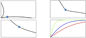
$\textrm{surface tension} = 81\ \textrm{dyn}\ \textrm{cm}^{-1} ; \textrm{density} = 1\ \textrm{gram}\ \textrm{cm}^{-3}$; water depth $h= 0.5$ cm. This leads to surface tension coefficient $\sigma \equiv$ surface tension/ density equals to $81\, \textrm{cm}^3\ \textrm{s}^{-2}$. Typical values for the wavenumbers are $k_1\approx 0.3\, \textrm{cm}^{-1}$; $k_2\approx 0.3\ \textrm{cm}^{-1}$ (marked as a full circle in figure 1a) and $k_3=k_1+k_2 \approx 0.6 \ \textrm{cm}^{-1}$. With these values at hand, we find $k_1h\approx 0.15; k_2h\approx 0.15$ and $k_3h\approx 0.3$ which represent a shallow-depth limit.(b) Finite depth:
$\textrm{surface tension} = 81\ \textrm{dyn}\ \textrm{cm}^{-1}; \textrm{density} = 1\ \textrm{gram}\ \textrm{cm}^{-3}$; water depth $h= 0.6$ cm. This results in $\sigma = 81\ \textrm{cm}^3\ \textrm{s}^{-2}$. In this case, we choose the following set of wavenumbers: $k_1\approx 1.5 \ \textrm{cm}^{-1}$; $k_2\approx 2\ \textrm{cm}^{-1}$ (indicated by a full circle in figure 1b) and $k_3=k_1+k_2 \approx 2.5\, \textrm{cm}^{-1}$. Thus, we have $k_1h\approx 0.9; k_2h\approx 1.2$ and $k_3h\approx 1.5$ which is a finite-depth regime.(c) Infinite depth:
$\textrm{surface tension} = 73\ \textrm{dyn}\ \textrm{cm}^{-1}; \textrm{density} = 1\ \textrm{gram}\ \textrm{cm}^{-3}$; water depth $h= 2$ cm and $\sigma = 73\ \textrm{cm}^{-3}\ \textrm{s}^{-2}$. Here, prototypical values for the wavenumbers are as follows: $k_1\approx 2.5 \ \textrm{cm}^{-1}$; $k_2\approx 2.6 \ \textrm{cm}^{-1}$ (shown by a full circle in figure 1c) and $k_3=k_1+k_2 \approx 5.1 \ \textrm{cm}^{-1}.$ In this case we find, $k_1h\approx 5; k_2h\approx 5.2$ and $k_3h\approx 10.2$ which fall into the limit of an infinite depth.
(ii) Two-dimensional case: illustrations.
(a) Shallow depth:
$\textrm{surface tension} = 73 \ \textrm{dyn}\ \textrm{cm}^{-1}; \textrm{density} = 1\ \textrm{gram}\ \textrm{cm}^{-3}$; water depth $h= 0.35$ cm and surface tension coefficient $\sigma$ equals to $73\ \textrm{cm}^3\ \textrm{s}^{-2}$. Typical values for the wavenumbers are $k_1 = | {\boldsymbol k}_1 | \approx 1\, \textrm{cm}^{-1}$; $k_2 = | {\boldsymbol k}_2 | \approx 0.54\, \textrm{cm}^{-1}$ (marked as a full circle in figure 2a) and $k_3= | {\boldsymbol k}_1 + {\boldsymbol k}_2 | \approx 1.54\, \textrm{cm}^{-1}$. With these values at hand, we find $k_1h\approx 0.35; k_2h\approx 0.19$ and $k_3h\approx 0.5$ which represent a shallow water limit.(b) Finite depth:
$\textrm{surface tension} = 73 \ \textrm{dyn}\ \textrm{cm}^{-1}; \textrm{density} = 1~\textrm{gram}/\textrm{cm}^3$; water depth $h= 0.6$ cm and $\sigma = 73\ \textrm{cm}^3\ \textrm{s}^{-2}$. Some prototypical values of wavenumbers are as follows: $k_1 = | {\boldsymbol k}_1 | \approx 2.1 \ \textrm{cm}^{-1}$; $k_2 = | {\boldsymbol k}_2 | \approx 1.9 \ \textrm{cm}^{-1}$ (marked as a full circle in figure 2b) and $k_3= | {\boldsymbol k}_1 + {\boldsymbol k}_2 | \approx 4 \ \textrm{cm}^{-1}$. With these values at hand, we find $k_1h\approx 1.3; k_2h\approx 1.1$ and $k_3h\approx 2.4$ which falls into the finite-depth fluid regime.(c) Infinite depth:
$\textrm{surface tension} = 73 \ \textrm{dyn}\ \textrm{cm}^{-1}; \textrm{density} = 1~\textrm{gram}/\textrm{cm}^3$; water depth $h=$ 2 cm and $\sigma = 73\ \textrm{cm}^3\ \textrm{s}^{-2}$. Example values of wavenumbers are as follows: $k_1 = | {\boldsymbol k}_1 | \approx 2.8\ \textrm{cm}^{-1}$; $k_2 = | {\boldsymbol k}_2 | \approx 2.3\ \textrm{cm}^{-1}$ (marked as a full circle in figure 2c) and $k_3= | {\boldsymbol k}_1 + {\boldsymbol k}_2 | \approx 5\, \textrm{cm}^{-1}.$ With these values at hand, we find $k_1h\approx 5.6; k_2h\approx 4.6$ and $k_3h\approx 10$ which falls into the infinite-depth case.


One-dimensional resonant triad curves satisfying the wavenumber–frequency resonance condition  $k_3=k_1+k_2$ and
 $\omega _3=\omega _1+\omega _2.$ All wavenumbers are measured in units of
 $\textrm{cm}^{-1}$ and depth
 $h$ in cm. The numerical values for the depth
 $h$ and surface tension used to produce the figure are respectively given by (a)
 $h=0.5\ \textrm{cm}$;
 $\sigma = 81\ \textrm{cm}^3\ \textrm{s}^{-2}$, (b)
 $h=0.6\ \textrm{cm}$;
 $\sigma = 81\ \textrm{cm}^3\ \textrm{s}^{-2}$ and (c)
 $h=2\ \textrm{cm}$;
 $\sigma = 73\ \textrm{cm}^3\ \textrm{s}^{-2}$. Shown in (d) is the graph of the tanh function for various values of depth. The full circles indicate typical wavenumber values leading to (a) shallow-depth limit with
 $k_1h\approx 0.15; k_2h\approx 0.15$ and
 $k_3h\approx 0.3$; (b) finite depth with
 $k_1h\approx 0.9; k_2h\approx 1.2$ and
 $k_3h\approx 1.5$; and (d) infinite-depth limit when
 $k_1h\approx 5; k_2h\approx 5.2$ and
 $k_3h\approx 10.2$.

One-dimensional resonant triad curves satisfying the wavenumber–frequency resonance condition  $k_3=k_1+k_2$ and
 $\omega _3=\omega _1+\omega _2.$ All wavenumbers are measured in units of
 $\textrm{cm}^{-1}$ and depth
 $h$ in cm. The numerical values for the depth
 $h$ and surface tension used to produce the figure are respectively given by (a)
 $h=0.475\ \textrm{cm}$;
 $\sigma = 73 \ \textrm{cm}^3\ \textrm{s}^{-2}$, (b)
 $h=0.52\ \textrm{cm}$;
 $\sigma = 73 \ \textrm{cm}^3\ \textrm{s}^{-2}$. The full circles indicate typical wavenumber values leading to (a) shallow-depth limit with
 $k_1h\approx 0.152; k_2h\approx 0.175$ and
 $k_3h\approx 0.33$; (b) finite depth with
 $k_1h\approx 0.75; k_2h\approx 0.75$ and
 $k_3h\approx 1.5$.

First, we will discuss typical values in the one-dimensional case. Figure 1 shows the existence of a numerical resonant triad for various values of depth: (a) shallow depth  $h= 0.5$ cm with
 $\sigma = 81 \ \textrm{cm}^3\ \textrm{s}^{-2}$, (b) finite depth
 $h=0.6$ cm, with
 $\sigma = 81 \ \textrm{cm}^3\ \textrm{s}^{-2}$ and (c) deep depth with
 $h= 2$ cm and
 $\sigma = 73 \ \textrm{cm}^3\ \textrm{s}^{-2}$. For convenience, we show in figure 1(d) a plot of the tanh function that helps identify various water depth limits. For completeness, in figure 2 we also show two more cases corresponding to shallow and finite-depth water limits with surface tension
 $\sigma = 73\ \textrm{cm}^3\ \textrm{s}^{-2}$.
Next, we discuss the two-dimensional case. Here, in all cases we take the surface tension coefficient to be  $\sigma = 73\ \textrm{cm}^3\ \textrm{s}^{-2}$. Figure 3 illustrates numerical resonant triad for various values of depth: (a) shallow depth
 $h= 0.35$ cm, (b) finite depth
 $h=0.6$ cm and (c) deep case with
 $h= 2$ cm. To help identify each limiting case we show in figure 2(d) a graph of the tanh as a function of the dimensionless parameter
 $kh.$
Two-dimensional resonant triad curves satisfying the wavenumber–frequency resonance condition  ${\boldsymbol k}_3={\boldsymbol k}_1+{\boldsymbol k}_2$ and
 $\omega _3=\omega _1+\omega _2.$ All wavenumbers are measured in units of
 $\textrm{cm}^{-1}$ and depth in cm. In all cases, the surface tension coefficient is taken to be
 $\sigma = 73 \ \textrm{cm}^3\ \textrm{s}^{-2}.$ The wavenumbers and depth are as follows: (a)
 $k_{1x}=k_{1y} = 0.7 \ \textrm{cm}^{-1}$ and depth
 $h=0.35\ \textrm{cm}$, (b)
 $k_{1x}=k_{1y} = 1.5 \ \textrm{cm}^{-1}$ and depth
 $h=0.6\ \textrm{cm}$, (c)
 $k_{1x}=k_{1y} = 2 \ \textrm{cm}^{-1}$ and depth
 $h=2\ \textrm{cm}$. Furthermore, we show in (d) the graph of tanh function for various values of depth
 $h$ that help identify the three limiting regimes of shallow, finite and deep depth. As is the case with figure 1, here, full circles indicate typical wavenumber values leading to (a) shallow-depth limit with
 $k_1h\approx 0.35; k_2h\approx 0.19$ and
 $k_3h\approx 0.5$; (b) finite depth with
 $k_1h\approx 1.3; k_2h\approx 1.1$ and
 $k_3h\approx 2.4$ and (d) infinite-depth limit when
 $k_1h\approx 5.6; k_2h\approx 4.6$ and
 $k_3h\approx 10.$

Gravity waves in fluids with different surface tension than pure water are included in our formulation. High surface tension fluids such as mercury in finite depth have been used in experiments to exhibit remarkable surface wave fluid phenomena. In Falcon, Laroche & Fauve (Reference Falcon, Laroche and Fauve2002), solitary waves on an air interface with mercury in shallow depth exhibit solitary waves of depression as opposed to solitary waves of elevation.
4. Six wave interaction in infinite depth
In this section we outline the derivation of the six wave equations in infinite depth starting from the non-local formulation of gravity waves as given by (2.9) and (2.10) up to order  $\epsilon.$ It is convenient to take the gradient of (2.10) and to define
 ${\boldsymbol {\nabla }} q \equiv {\boldsymbol Q}= (Q_1,Q_2).$ With this definition, we find the following equations to order
 $\epsilon$:
 \begin{gather} \int_{\mathbb{R}^2} \,{\rm d} {\boldsymbol r} {\rm e}^{ -{\rm i} {\boldsymbol k}\ \boldsymbol{\cdot}\ {\boldsymbol r}} ( 1+ \epsilon k \eta) \left( {\rm i}\eta_t - \frac{ {\boldsymbol k} \boldsymbol{\cdot} {\boldsymbol Q} }{k} \right) =0, \end{gather}
 \begin{gather} {\boldsymbol Q}_{t} + g {\boldsymbol{\nabla}} \eta + \frac{ \epsilon}{2} {\boldsymbol{\nabla}} \left( |{\boldsymbol Q}|^2 - \eta_t^2 \right) = \sigma {\nabla}^2 {\boldsymbol{\nabla}} \eta. \end{gather}
We can eliminate the  ${\boldsymbol Q}$ variable from (4.1) by taking the time derivative of (4.1) and then substituting the expression for
 ${\boldsymbol Q}_{t}$ from (4.2) back into the resulting system. This yields (to first order in
 $\epsilon$)
 $$\begin{align} &\int_{\mathbb{R}^2}
\,{\rm d} {\boldsymbol r} {\rm e}^{ -{\rm i} {\boldsymbol k}\ \boldsymbol{\cdot}\ {\boldsymbol r}} \left\{ {\rm
i}\eta_{tt} + \frac{ {\boldsymbol k}}{k} \boldsymbol{\cdot}
(g {\boldsymbol{\nabla}} \eta -\sigma {\nabla}^2
{\boldsymbol{\nabla}} \eta )\right. \nonumber\\ &\quad \left.+\,\epsilon \left(\frac{{\boldsymbol k}}{2 k}
\boldsymbol{\cdot} {\boldsymbol{\nabla}} ( |{\boldsymbol
Q}|^2 - \eta_t^2 ) +{\rm i} k (\eta \eta_t)_t-
({\boldsymbol k} \boldsymbol{\cdot} {\boldsymbol Q }\eta)_t
\right) \right\}=0 . \end{align}$$
Here, we will use a space–time multiple scale perturbation procedure to find the six wave interaction equations. Before doing so, it is important to mention that most applications of multiple scale asymptotic expansion is done within the framework of ordinary or partial differential equations. This is in sharp contrast to our case where now multiple scale method is being applied on system of equations of an integral type which further complicates the process of scale separation. As such, a new approach should be adapted. In fact, similar situation has been previously encountered by Ablowitz & Haut Terry (Reference Ablowitz and Haut Terry2009) in their study of two fluid layers. To this end, we introduce a slow space–time scales  ${\boldsymbol R}=\epsilon {\boldsymbol r}, T= \epsilon t$ and assume that the wave elevation and velocity potential to depend on both the fast and slow variables, i.e.
 $\eta = \eta ({\boldsymbol r}, t, {\boldsymbol R}, T; \epsilon ) \textrm{~and~} Q= Q({\boldsymbol r}, t, {\boldsymbol R}, T;\epsilon )$. Substituting the asymptotic expansion
 $\eta = \eta ^{(0)} + \epsilon \eta ^{(1)} + \cdots, Q = Q^{(0)} + \epsilon Q^{(1)} + \cdots$ and the transformation
 ${\boldsymbol {\nabla }} \rightarrow {\boldsymbol {\nabla }}_{\boldsymbol r}+\epsilon {\boldsymbol {\nabla }}_{\boldsymbol R}; ~~\partial _t ~ \rightarrow ~ \partial _t+\epsilon \partial _T$ into (4.3) leads to a hierarchy of equations at each order in
 $\epsilon$. For example, the ‘leading’-order equation (that has no apparent order-
 $\epsilon$ terms in it) takes the form
 \begin{equation} L_{{\boldsymbol k}}[\eta^{(0)}] \equiv \int_{\mathbb{R}^2} \,{\rm d} {\boldsymbol r} {\rm e}^{ -{\rm i} {\boldsymbol k}\ \boldsymbol{\cdot}\ {\boldsymbol r}} \left[ {\rm i}\eta^{(0)}_{tt} + \frac{ {\boldsymbol k}}{k} \boldsymbol{\cdot} \left(g {\boldsymbol{\nabla}}_{\boldsymbol r} \eta^{(0)} -\sigma \boldsymbol{\nabla}_{\boldsymbol r}^2 {\boldsymbol{\nabla}}_{\boldsymbol r} \eta^{(0)} \right) \right] =0 . \end{equation}
For the type of wave elevation  $\eta ^{(0)}$ considered in this paper (such as those that have a slowly varying amplitude and a carrier wave which are of the form given by (1.1)), this ‘leading’-order contributions, i.e. (4.4), could include in it ‘hidden’ higher-order contributions in powers of
 $\epsilon.$ This is the case due to the presence of an integral in (4.4) and, hence, lack of full separation of scales. This can be clearly seen by examining a typical term in the hierarchy that looks like
 \begin{equation} I \equiv \int_{\mathbb{R}^2} \,{\rm d} {\boldsymbol r}' {\rm e}^{ -{\rm i} {\boldsymbol k}\ \boldsymbol{\cdot}\ {\boldsymbol r}'} G({\boldsymbol k}) f({\boldsymbol R}',T) \exp({ {\rm i} s({\boldsymbol k}_0 \boldsymbol{\cdot} {\boldsymbol r}' - \omega_0t)}) , \end{equation}
where  ${\boldsymbol k}_0 , \omega _0$ belongs to the set of resonant wavenumbers and frequencies;
 ${\boldsymbol R}' \equiv \epsilon {\boldsymbol r}'$ and
 $s=\pm 1.$ Multiplying (4.5) by
 $\exp (\textrm{i} {\boldsymbol k} \boldsymbol {\cdot } {\boldsymbol r})$ and integrating over the
 ${\boldsymbol k}$ variable gives
 \begin{equation} \tilde{I} = {\rm e}^{ -{\rm i}s \omega_0 t } \int_{\mathbb{R}^2} \int_{\mathbb{R}^2} \,{\rm d} {\boldsymbol r}' \,{\rm d} {\boldsymbol k} {\rm e}^{ {\rm i} {\boldsymbol k}\ \boldsymbol{\cdot}\ {\boldsymbol r}} G({\boldsymbol k}) f({\boldsymbol R}',T) \exp({ - {\rm i} ({\boldsymbol k} - s{\boldsymbol k}_0) \boldsymbol{\cdot} {\boldsymbol r}'}) . \end{equation}
Next, introduce the change of variables:  ${\boldsymbol k} - s{\boldsymbol k}_0 \equiv \epsilon {\boldsymbol K}$ and
 ${\boldsymbol R} \equiv \epsilon {\boldsymbol r}.$ With this, (4.6) becomes
 \begin{align} \tilde{I} &= \exp({ {\rm i} s({\boldsymbol k}_0 \boldsymbol{\cdot} {\boldsymbol r} - \omega_0t)}) \int_{\mathbb{R}^2} \int_{\mathbb{R}^2} \,{\rm d} {\boldsymbol R}' \,{\rm d} {\boldsymbol K} {\rm e}^{ {\rm i} {\boldsymbol K} \boldsymbol{\cdot} {\boldsymbol R}} G( s{\boldsymbol k}_0 + \epsilon {\boldsymbol K}) f({\boldsymbol R}' ,T) {\rm e}^{ - {\rm i} {\boldsymbol K} \boldsymbol{\cdot} {\boldsymbol R}'} \nonumber\\ &= \exp({ {\rm i} s({\boldsymbol k}_0 \boldsymbol{\cdot} {\boldsymbol r} - \omega_0t)}) \int_{\mathbb{R}^2} \,{\rm d} {\boldsymbol K} G( s{\boldsymbol k}_0 + \epsilon {\boldsymbol K}) \hat{f} ({\boldsymbol K} ,T) {\rm e}^{ {\rm i} {\boldsymbol K} \boldsymbol{\cdot} {\boldsymbol R}}. \end{align}
In the above,  $\hat {f}$ denotes the two-dimensional Fourier transform of
 $f$ defined by
 \begin{equation} \hat{f} ({\boldsymbol k}) = F[f] \equiv \int_{\mathbb{R}^2} \,{\rm d} {\boldsymbol r} {\rm e}^{ -{\rm i} {\boldsymbol k}\ \boldsymbol{\cdot}\ {\boldsymbol r}} f( {\boldsymbol r}) . \end{equation}
Finally, replacing  $G( s{\boldsymbol k}_0 + \epsilon {\boldsymbol K})$ in (4.7) by its first-order approximation
 $G( s{\boldsymbol k}_0) + \epsilon {\boldsymbol K} \boldsymbol {\cdot } \boldsymbol {\nabla }_{{\boldsymbol k}} G( s{\boldsymbol k}_0)$ and
 ${\boldsymbol K}f( {\boldsymbol r})$ by
 $-\textrm{i}\boldsymbol {\nabla }_{{\boldsymbol R}} f$ we find
 \begin{equation} \tilde{I} = 2{\rm \pi} \exp({ {\rm i} s({\boldsymbol k}_0 \boldsymbol{\cdot} {\boldsymbol r} - \omega_0t)}) \left( G( s{\boldsymbol k}_0)~ f({\boldsymbol R},T) - {\rm i} \epsilon \boldsymbol{\nabla}_{{\boldsymbol k}} G (s{\boldsymbol k}_0) \boldsymbol{\cdot} \boldsymbol{\nabla}_{{\boldsymbol R}} f + O(\epsilon^2)\right) . \end{equation}
The consequences of (4.9) are twofold: (i) it allows one to identify any ‘hidden’ contributions in powers of  $\epsilon$ that otherwise are absent and (ii) it provides a mechanism to get rid of the integral that appears in (4.5) by replacing it with its equivalent differential form. The latter is vital in deriving the six wave interaction system.
The three resonant wave ansatze for the wave elevation considered throughout this paper is given by
 \begin{equation} \eta^{(0)}({\boldsymbol r} , t; {\boldsymbol R} , T) = \sum_{j=1}^3 \left( A_j ({\boldsymbol R},T) {\rm e}^{-{\rm i} \theta_j} +B_j({\boldsymbol R},T) {\rm e}^{{\rm i} \theta_j} \right), \end{equation}
where  $\theta _j \equiv {\boldsymbol k}_j \boldsymbol {\cdot } {\boldsymbol r} - \omega _j t, \omega _j=\omega (k_j), k_j = |{\boldsymbol k}_j| .$ Then
 \begin{equation} L_{{\boldsymbol k}}[G({\boldsymbol k}) \eta^{(0)}] = 0. \end{equation}
Furthermore, for the ansatz given in (4.10) we find  $G({\boldsymbol k}) = \textrm{i}[- \omega _j^2 +s {\boldsymbol k} \boldsymbol {\cdot } {\boldsymbol k}_j( g + \sigma | {\boldsymbol k}_j |^2 )/k], s= \pm 1$ and
 $k= | {\boldsymbol k} |$. Note that
 $\boldsymbol {\nabla }_{{\boldsymbol k}} G (s{\boldsymbol k}_j) = 0$ hence, no higher order in powers of
 $\epsilon$ are present in (4.4). Furthermore,
 $G (s{\boldsymbol k}_j) = 0$ whenever, the frequency
 $\omega$ satisfies the infinite-depth water wave dispersion given in (1.4). The leading-order solution for
 ${\boldsymbol Q}$ is obtained from linearizing (4.2). This yields
 \begin{equation} {\boldsymbol Q}^{(0)}({\boldsymbol r} ,t,{\boldsymbol R},T) = \sum_{j=1}^3 ~ \frac{ \omega_j {\boldsymbol k}_j }{k_j} \left( A_j({\boldsymbol R},T) {\rm e}^{-{\rm i} \theta_j}+ B_j({\boldsymbol R},T) {\rm e}^{{\rm i} \theta_j} \right) . \end{equation}
Next, we analyse the order- $\epsilon$ equation given by
 $$\begin{align}
- L_{{\boldsymbol k}}[\eta^{(1)}] &= \int_{\mathbb{R}^2}
\,{\rm d} {\boldsymbol r} {\rm e}^{ -{\rm i} {\boldsymbol k}\ \boldsymbol{\cdot}\ {\boldsymbol r}} \left[ 2{\rm i}
\eta^{(0)}_{tT} + \frac{ {\boldsymbol k}}{k}
\boldsymbol{\cdot} \left(g
{\boldsymbol{\nabla}}_{\boldsymbol R} \eta^{(0)} - \sigma
\boldsymbol{\nabla}_{\boldsymbol r}^2
{\boldsymbol{\nabla}}_{\boldsymbol R} \eta^{(0)}\right.\right.\nonumber\\
&\quad\left.\left. - \,2 \sigma
( \boldsymbol{\nabla}_{\boldsymbol r} \boldsymbol{\cdot}
{\boldsymbol{\nabla}}_{\boldsymbol R} )
\boldsymbol{\nabla}_{\boldsymbol r} \eta^{(0)} \vphantom{\frac{1}{2}}\right)
\right]\nonumber\\
&\quad + \int_{\mathbb{R}^2} \,{\rm d}
{\boldsymbol r} {\rm e}^{ -{\rm i} {\boldsymbol k}\ \boldsymbol{\cdot}\ {\boldsymbol r}}
\left(\frac{{\boldsymbol k}}{2 k} \boldsymbol{\cdot}
{\boldsymbol{\nabla}}_{{\boldsymbol r}} ( |{\boldsymbol
Q}^{(0)}|^2 - (\eta_t^{(0)})^2 ) + {\rm i} k
\left(\eta^{(0)}_t \eta^{(0)}\right)_t\right.\nonumber\\
&\quad \left. - \,{\boldsymbol k}
\boldsymbol{\cdot} \left({\boldsymbol Q}^{(0)}
\eta^{(0)}\right)_t \right).
\end{align}$$
Substituting (4.10) and (4.12) gives rise to a linear non-homogeneous equation that exhibits secular terms proportional to  $\exp (\textrm{i} s \theta _j)$ with wavenumbers
 ${\boldsymbol k}_j$ and corresponding frequencies
 $\omega _j=\omega ({\boldsymbol k}_j), j=1,2,3$ satisfying the resonance triad condition (3.1). In terms of the phases
 $\theta _j$ the resonance relation takes the alternative form
 \begin{equation} \theta_3 = \theta_1 + \theta_2 . \end{equation}
The conditions that guarantee removal of such terms leads to the following six wave interaction equations (valid for infinite water depth):
 $$\begin{gather} 2 v^I_{p_1} \left( \partial_T + {\boldsymbol C}^{I}_1 \boldsymbol{\cdot} {\boldsymbol{\nabla}}_{\boldsymbol R} \right ) A_1 - {\rm i} \gamma^{I} B_2 A_3=0 , \end{gather}$$
 $$\begin{gather}2 v^I_{p_2} \left( \partial_T + {\boldsymbol C}^{I}_2 \boldsymbol{\cdot} {\boldsymbol{\nabla}}_{\boldsymbol R} \right ) A_2 - {\rm i} \gamma^{I} B_1 A_3=0 , \end{gather}$$
 $$\begin{gather}2 v^I_{p_3} \left( \partial_T + {\boldsymbol C}^{I}_3 \boldsymbol{\cdot} {\boldsymbol{\nabla}}_{\boldsymbol R} \right ) A_3 - {\rm i} \gamma^{I} A_1 A_2=0 , \end{gather}$$
 $$\begin{gather}2 v^I_{p_1} \left( \partial_T + {\boldsymbol C}^{I}_1 \boldsymbol{\cdot} {\boldsymbol{\nabla}}_{\boldsymbol R} \right ) B_1 + {\rm i} \gamma^{I} B_3 A_2=0 , \end{gather}$$
 $$\begin{gather}2 v^I_{p_2} \left( \partial_T + {\boldsymbol C}^{I}_2 \boldsymbol{\cdot} {\boldsymbol{\nabla}}_{\boldsymbol R} \right ) B_2 + {\rm i} \gamma^{I} B_3 A_1=0 , \end{gather}$$
 $$\begin{gather}2 v^I_{p_3} \left( \partial_T + {\boldsymbol C}^{I}_3 \boldsymbol{\cdot} {\boldsymbol{\nabla}}_{\boldsymbol R} \right ) B_3 + {\rm i} \gamma^{I} B_1 B_2=0 , \end{gather}$$
where  ${\boldsymbol C}^{I}_j \equiv {\boldsymbol {\nabla }}_{{\boldsymbol k}} \omega (k_j)$ and
 $v^I_{p_j} \equiv \omega (k_j) / k_j$ are the group and phase velocities, respectively;
 $\gamma ^{I}$ denotes the nonlinear coefficient corresponding to the infinite-depth case (see the Appendix)
 \begin{align} \gamma^I = \ \omega_1 \omega_2 {\boldsymbol e}_1 \boldsymbol{\cdot} {\boldsymbol e}_2 + \omega_1 \omega_3 {\boldsymbol e}_1 \boldsymbol{\cdot} {\boldsymbol e}_3 + \omega_2 \omega_3 {\boldsymbol e}_2 \boldsymbol{\cdot} {\boldsymbol e}_3 + \omega_1 \omega_2 - \omega_1 \omega_3 - \omega_2 \omega_3 ,\quad {\boldsymbol e}_j\equiv {\boldsymbol k}_j/k_j. \end{align}
For the one-dimensional case for which  ${\boldsymbol e}_1 \boldsymbol {\cdot } {\boldsymbol e}_2 = 1, {\boldsymbol e}_1 \boldsymbol {\cdot } {\boldsymbol e}_3 = 1$ and
 ${\boldsymbol e}_2 \boldsymbol {\cdot } {\boldsymbol e}_3 =1$ we find
 $\gamma ^I = 2 \omega _1 \omega _2$ When
 $B_j=A_j ^*$ the resulting equations agree with those given by Simmons (Reference Simmons1969).
5. Six wave interaction in finite depth
In this section we turn our attention to the study of the six wave resonant interaction system corresponding to the finite-depth wave limit. The mathematical derivation closely follows the infinite-depth case with the exception that the model coefficients are now dependent on the depth  $h$. We begin by taking the time derivative of the non-local (2.8) for finite depth that contains in it the
 $O(1)$ and
 $O(\epsilon )$ terms. This yields (recall that
 ${\boldsymbol Q }\equiv \boldsymbol {\nabla } q$)
 \begin{align} \int_{\mathbb{R}^2} \,{\rm d} {\boldsymbol r} {\rm e}^{ -{\rm i} {\boldsymbol k}\ \boldsymbol{\cdot}\ {\boldsymbol r}} \left\{ {\rm i}\eta_{tt} - \frac{ \tanh(k h) }{k} {\boldsymbol k} \boldsymbol{\cdot} {\boldsymbol Q}_t + \epsilon\left[ {\rm i} k \tanh(k h) (\eta\eta_t)_t -({\boldsymbol k} \boldsymbol{\cdot} {\boldsymbol Q }\eta)_t \right] \right \} + O(\epsilon^2) =0. \end{align}
We substitute the free surface Bernoulli equation (4.2) for  ${\boldsymbol Q}_t$ (which is valid for the finite-depth case as well) back into (5.1) to find
 $$\begin{align} &\int_{\mathbb{R}^2}
\,{\rm d} {\boldsymbol r} {\rm e}^{ -{\rm i} {\boldsymbol k}\ \boldsymbol{\cdot}\ {\boldsymbol r}} \left\{ {\rm
i}\eta_{tt} + \frac{ \tanh (kh)}{k} {\boldsymbol k}
\boldsymbol{\cdot} (g {\boldsymbol{\nabla}} \eta -\sigma
{\nabla}^2 {\boldsymbol{\nabla}} \eta ) \right. \nonumber\\
&\quad +\,\left. \epsilon \left( \frac{ \tanh (kh) }{2 k}
{\boldsymbol k} \boldsymbol{\cdot} {\boldsymbol{\nabla}} (
|{\boldsymbol Q}|^2 - \eta_t^2 ) + {\rm i} k \tanh (k h)
(\eta \eta_t)_t - ({\boldsymbol k} \boldsymbol{\cdot}
{\boldsymbol Q }\eta)_t \right) \right\}=0 .
\end{align}$$
Next, we employ a space–time multiple scale perturbative expansion to isolate the ‘leading’ and order- $\epsilon$ equations for the wave amplitude and velocity potential. In this regard, the integral-to-differential formulation presented in (4.5)–(4.9) is used to identify any ‘hidden’ order-
 $\epsilon$ contributions that could be embedded in the ‘leading’-order equation. With this at hand, the ‘leading’-order equation reads
 \begin{equation} L^h_{{\boldsymbol k}}[\eta^{(0)}] \equiv \int_{\mathbb{R}^2} \,{\rm d} {\boldsymbol r} {\rm e}^{ -{\rm i} {\boldsymbol k}\ \boldsymbol{\cdot}\ {\boldsymbol r}} \left[ {\rm i}\eta^{(0)}_{tt} + \frac{ \tanh (kh)}{k} {\boldsymbol k} \boldsymbol{\cdot} \left(g {\boldsymbol{\nabla}}_{\boldsymbol r} \eta^{(0)} -\sigma \boldsymbol{\nabla}_{\boldsymbol r}^2 {\boldsymbol{\nabla}}_{\boldsymbol r} \eta^{(0)} \right) \right] =0 . \end{equation}
The three wave form (4.10) would transform (5.3) into the integral representation given by (4.5) with  $G({\boldsymbol k}) = \textrm{i}[- \omega _j^2 +s \tanh (kh) ( g + \sigma k_j^2 ) {\boldsymbol k} \boldsymbol {\cdot } {\boldsymbol k}_j /k], s= \pm 1$ and
 $k= | {\boldsymbol k} |$. Additionally, we find
 \begin{equation} \boldsymbol{\nabla}_{{\boldsymbol k}} G (s{\boldsymbol k}_j) = {\rm i} ( g k_j + \sigma k_j^3 ) \boldsymbol{\nabla}_{{\boldsymbol k}} \tanh(kh)|_{{\boldsymbol k}=s{\boldsymbol k}_j} \ne 0 . \end{equation}
There are two important implications emanating from (5.4) especially in conjunction with (4.9). The first is concerned with the identification of the genuine leading-order contribution that takes the form  $G (s{\boldsymbol k}_j) = 0.$ The latter is always satisfied so long the frequency
 $\omega _j$ follows the finite-depth wave dispersion relation (2.11). The associated eigenfunction (wave elevation) remains unchanged while the velocity potential assumes the new form
 \begin{equation} {\boldsymbol Q}^{(0)}({\boldsymbol r} ,t,{\boldsymbol R},T) = \sum_{j=1}^3 \frac{ \omega_j {\boldsymbol k}_j }{k_j \tanh (k_jh)} \left ( A_j({\boldsymbol R},T) {\rm e}^{-{\rm i} \theta_j} + B_j({\boldsymbol R},T) {\rm e}^{{\rm i} \theta_j} \right) . \end{equation}
Secondly, as a consequence of (5.4) the order- $\epsilon$ equation for
 $\eta ^{(1)}$ now acquires a new term which is proportional to
 $\boldsymbol {\nabla }_{{\boldsymbol k}} G (s{\boldsymbol k}_j)$
 \begin{align}
- L^h_{{\boldsymbol k}}[\eta^{(1)}] & =
\int_{\mathbb{R}^2} \,{\rm d} {\boldsymbol r} {\rm e}^{
-{\rm i} {\boldsymbol k}\ \boldsymbol{\cdot}\ {\boldsymbol r}} \left[ 2{\rm i} \eta^{(0)}_{tT} + \frac{ \tanh(kh) }{k}
{\boldsymbol k} \boldsymbol{\cdot} \left(g
{\boldsymbol{\nabla}}_{\boldsymbol R} \eta^{(0)} - \sigma
\boldsymbol{\nabla}_{\boldsymbol r}^2
{\boldsymbol{\nabla}}_{\boldsymbol R} \eta^{(0)}\right.\right.\nonumber\\
&\quad \left.\left. -\, 2 \sigma ( \boldsymbol{\nabla}_{\boldsymbol r} \boldsymbol{\cdot}
{\boldsymbol{\nabla}}_{\boldsymbol R} )
\boldsymbol{\nabla}_{\boldsymbol r} \eta^{(0)} \right)
\right. \nonumber\\ &\quad -\, \left. {\rm i}
\boldsymbol{\nabla}_{{\boldsymbol k}} G
\boldsymbol{\cdot} \boldsymbol{\nabla}_{{\boldsymbol R}}
\eta^{(0)} + \frac{ \tanh(kh) }{2 k} {\boldsymbol k}
\boldsymbol{\cdot} {\boldsymbol{\nabla}}_{{\boldsymbol
r}} \left( |{\boldsymbol Q}^{(0)}|^2 - (\eta_t^{(0)})^2
\right) \right. \nonumber\\ &\quad +\, \left. {\rm i} k
\tanh(kh) \left(\eta^{(0)}_t \eta^{(0)}\right)_t -
{\boldsymbol k} \boldsymbol{\cdot} \left({\boldsymbol
Q}^{(0)} \eta^{(0)}\right)_t \vphantom{\frac{1}{2}}\right].
\end{align}
Substituting (4.10) and (5.5) into (4.13) gives rise to a non-homogeneous integral equation whose solvability condition (boundedness of the associated eigenfunctions) determines the six wave interactions equations. They are given by
 $$\begin{gather} 2 v^F_1 \left( \partial_T + {\boldsymbol C}^{F}_1 \boldsymbol{\cdot} {\boldsymbol{\nabla}}_{\boldsymbol R} \right ) A_1 - {\rm i} \gamma^{F} B_2 A_3=0 , \end{gather}$$
 $$\begin{gather}2 v^F_2 \left( \partial_T + {\boldsymbol C}^{F}_2 \boldsymbol{\cdot} {\boldsymbol{\nabla}}_{\boldsymbol R} \right ) A_2 - {\rm i} \gamma^{F} B_1 A_3=0 , \end{gather}$$
 $$\begin{gather}2 v^F_3 \left( \partial_T + {\boldsymbol C}^{F}_3 \boldsymbol{\cdot} {\boldsymbol{\nabla}}_{\boldsymbol R} \right ) A_3 - {\rm i} \gamma^{F} A_1 A_2=0 , \end{gather}$$
 $$\begin{gather}2 v^F_1 \left( \partial_T + {\boldsymbol C}^{F}_1 \boldsymbol{\cdot} {\boldsymbol{\nabla}}_{\boldsymbol R} \right ) B_1 + {\rm i} \gamma^{F} B_3 A_2=0 , \end{gather}$$
 $$\begin{gather}2 v^F_2 \left( \partial_T + {\boldsymbol C}^{F}_2 \boldsymbol{\cdot} {\boldsymbol{\nabla}}_{\boldsymbol R} \right ) B_2 + {\rm i} \gamma^{F} B_3 A_1=0 , \end{gather}$$
 $$\begin{gather}2 v^F_3 \left( \partial_T + {\boldsymbol C}^{F}_3 \boldsymbol{\cdot} {\boldsymbol{\nabla}}_{\boldsymbol R} \right ) B_3 + {\rm i} \gamma^{F} B_1 B_2=0 , \end{gather}$$
where  ${\boldsymbol C}^F_j= \boldsymbol {\nabla }_{{\boldsymbol k}} \omega ( {\boldsymbol k}={\boldsymbol k}_j)$ is the group velocity;
 $v^F_j \equiv \omega ({\boldsymbol k}_j)/[k_j \tanh ( k_j h )]$ and
 $\gamma ^{F}$ is the nonlinear coupling coefficient respectively given by
 $$\begin{gather}
{\boldsymbol C}^F_j = \frac{(g + 3\sigma k_j^2) \tanh ( k_j
h ) {\boldsymbol k}_j}{2 k_j \omega_j} + \frac{ h (g +
\sigma k_j^2) {\rm sech}^2 ( k_j h ) {\boldsymbol k}_j}{2
\omega_j} ,
\end{gather}$$
 $$\begin{gather}\gamma^F = \frac{\omega_1 \omega_2
{\boldsymbol e}_1 \boldsymbol{\cdot} {\boldsymbol
e}_2}{\tanh ( k_1 h ) \tanh ( k_2 h )} + \frac{\omega_1
\omega_3 {\boldsymbol e}_1 \boldsymbol{\cdot}
{\boldsymbol e}_3}{\tanh ( k_1 h ) \tanh ( k_3 h )} +
\frac{\omega_2 \omega_3 {\boldsymbol e}_2
\boldsymbol{\cdot} {\boldsymbol e}_3}{\tanh ( k_2 h )
\tanh ( k_3 h )}\nonumber\\
+\, \omega_1 \omega_2 - \omega_1 \omega_3 - \omega_2 \omega_3 .
\end{gather}$$
The above equations are equivalent to the six wave equations (1.8) by taking  $\sigma _j=\gamma ^{F}/(2\nu ^{F}_j), j=1,2,3$. We next discuss various important limiting cases such as the infinite and shallow depth.
Infinite depth
This amounts to taking the  $h \rightarrow \infty$ in (5.14) recovering the result given in (4.21).
Shallow-depth limit
This is an interesting and important case that also apparently has not been studied in the literature. This amount to ‘small’ depth  $h$ such that
 $\tanh ( k_j h ) \approx hk_j.$ In this limit the six wave interaction shallow-depth equations are given by
 $$\begin{gather} \frac{2\omega_1}{ k_1^2 h } \left( \partial_T + {\boldsymbol C}^{S}_1 \boldsymbol{\cdot} {\boldsymbol{\nabla}}_{\boldsymbol R} \right ) A_1 - {\rm i} \gamma^S B_2 A_3=0 , \end{gather}$$
 $$\begin{gather}\frac{2\omega_2}{ k_2^2 h} \left( \partial_T + {\boldsymbol C}^{S}_2 \boldsymbol{\cdot} {\boldsymbol{\nabla}}_{\boldsymbol R} \right ) A_2 - {\rm i} \gamma^S B_1 A_3=0 , \end{gather}$$
 $$\begin{gather}\frac{2\omega_3}{ k_3^2 h} \left( \partial_T + {\boldsymbol C}^{S}_3 \boldsymbol{\cdot} {\boldsymbol{\nabla}}_{\boldsymbol R} \right ) A_3 - {\rm i} \gamma^S A_1 A_2=0 , \end{gather}$$
 $$\begin{gather}\frac{2\omega_1}{ k_1^2 h} \left( \partial_T + {\boldsymbol C}^{S}_1 \boldsymbol{\cdot} {\boldsymbol{\nabla}}_{\boldsymbol R} \right ) B_1 + {\rm i} \gamma^S B_3 A_2=0 , \end{gather}$$
 $$\begin{gather}\frac{2\omega_2}{ k_2^2h} \left( \partial_T + {\boldsymbol C}^{S}_2 \boldsymbol{\cdot} {\boldsymbol{\nabla}}_{\boldsymbol R} \right ) B_2 + {\rm i} \gamma^S B_3 A_1=0 , \end{gather}$$
 $$\begin{gather}\frac{2\omega_3}{ k_3^2h} \left( \partial_T + {\boldsymbol C}^{S}_3 \boldsymbol{\cdot} {\boldsymbol{\nabla}}_{\boldsymbol R} \right ) B_3 + {\rm i} \gamma^S B_1 B_2=0 , \end{gather}$$
where, as  $h\to 0$, the dispersion relation is given by
 \begin{equation} \omega^2= (gk^2+\sigma k^4)h . \end{equation}
With this at hand, the group velocity and nonlinear coefficient are given by
 \begin{equation} {\boldsymbol C}^S_j = \frac{ h(g + 2\sigma k_j^2) {\boldsymbol k}_j}{\omega_j} , \end{equation}
and
 $$\begin{align} \gamma^S &=
\frac{\omega_1 \omega_2 {\boldsymbol e}_1
\boldsymbol{\cdot} {\boldsymbol e}_2}{ (k_1 h) (k_2 h) } +
\frac{\omega_1 \omega_3 {\boldsymbol e}_1
\boldsymbol{\cdot} {\boldsymbol e}_3}{( k_1 h )( k_3 h )} +
\frac{\omega_2 \omega_3 {\boldsymbol e}_2
\boldsymbol{\cdot} {\boldsymbol e}_3}{ (k_2 h)(k_3 h)}
\nonumber\\ &\quad + \omega_1 \omega_2 - \omega_1 \omega_3 -
\omega_2 \omega_3 . \end{align}$$
Equations (5.15)–(5.20) comprise the shallow-depth six wave interaction equations. While written in this form they have the depth  $h$ in them, they can be rescaled to eliminate this dependence.
6. Conclusion
Multi wave parametric resonant interactions are ubiquitous in nonlinear sciences. They occur in a wide range of physical settings beyond gravity waves; e.g. optics, plasma physics and other areas of fluid mechanics to name a few. Generally speaking, they form when two or more waves with wavenumbers  $k_j$ and corresponding frequencies
 $\omega _j$ ‘add up’ to generate a new wave form with wavenumber
 $k_n$ and frequency
 $\omega _n$ that satisfy the resonant condition:
 $\omega _n=\sum _j\omega _j$ and
 $k_n=\sum _j k_j.$ We also remark that such parametric processes find application in nonlinear optics where second and third harmonic generations are used for frequency conversion (Buryak et al. Reference Buryak, Di Trapani, Skryabin and Trillo2002). In fluid mechanics on the other hand, they are sometimes utilized to explain formation of rogue waves (Yang & Yang Reference Yang and Yang2022, Reference Yang and Yang2021).
Of particular interest are the three wave resonant triad interactions which occur on an order  $1/\epsilon$ time scale where
 $\epsilon$ is a measure of nonlinearity. Mathematically speaking, they form a coupled system of three first-order quadratically nonlinear evolution equations in two space one time dimension. As mentioned in the introduction, they were first derived by Simmons (Reference Simmons1969) in the context of deep-depth waves. Later, they were shown to be exactly solvable in 1975 by Ablowitz & Haberman (Reference Ablowitz and Haberman1975a) using inverse scattering transform methods. Importantly, their integrability was established by introducing a system of six wave interactions whose integrable symmetry reduction leads to the same three wave equations as Simmons found.
In this paper we show that the six wave interaction system found by Ablowitz & Haberman, in the context of integrability theory, can be derived from the equations of classical gravity waves. Rather than employing the depth-dependent equations of water waves ((2.1)–(2.4)) we use the Ablowitz–Fokas–Musslimani (Ablowitz et al. Reference Ablowitz, Fokas and Musslimani2006) (2+1)-dimensional non-local reformulation and solve for the free surface variables of gravity waves; see ((2.5)–(2.6)). This has the advantage of reducing some of the tedious algebra. From this this formulation the six wave interaction equations satisfying triad resonance conditions are obtained in both finite and infinite-depth cases. The shallow-depth limit is also considered. The derivation has several steps: (i) introduce a small amplitude wave elevation and velocity potential via a small parameter  $0 < \epsilon \ll 1$ and recast the non-local equations in terms of the new variables. (ii) Expand the resulting system and keep terms up to order
 $\epsilon$. (iii) Implement a space–time multiple scale perturbation expansion. Since the equations are non-local one must carefully consider how to apply multiscale methods. Equations ((4.5)–(4.9)) are used here to transform non-local equations to differential equations and hence achieve full scale separation. (iv) Make a three wave ansatz for the wave amplitude and velocity potential. (v) Remove all secular terms at the order-
 $\epsilon$ equation and obtain the desired system of six waves equations. As a closing remark, we point out that the six wave system admits a generalized integrable non-local symmetry reductions in the form
 $r(x,t) = \sigma q(x_0-x,t_0-t)$ with arbitrary real parameters
 $x_0,t_0$ (Ablowitz & Musslimani Reference Ablowitz and Musslimani2021). This in turn leads to a new system of interacting shifted three wave system whose study is left for a future work.
Funding
This work was partially supported by NSF under grant DMS-2005343 and NSFC under grant number 12101590.
Declaration of interests
The authors report no conflict of interest.
Appendix A
Here, we provide a detailed account of the derivation of the six wave equations for infinite depth in particular deriving the linear and nonlinear coefficients that appear in (4.15)–(4.20). To start with, note that the right-hand side of (4.13) has two contributing factors: (i) linear and (ii) nonlinear. Substituting (4.10) into (4.13) and using the integral-differential identity discussed in (4.5)–(4.9) (that allows one to transform the integral to differential form) we find
 \begin{align}
\text{linear terms} &\equiv 2{\rm i} \eta^{(0)}_{tT} +
\frac{ {\boldsymbol k}}{k} \boldsymbol{\cdot} (g
{\boldsymbol{\nabla}}_{\boldsymbol R} \eta^{(0)} - \sigma
\boldsymbol{\nabla}_{\boldsymbol r}^2
{\boldsymbol{\nabla}}_{\boldsymbol R} \eta^{(0)} - 2 \sigma
( \boldsymbol{\nabla}_{\boldsymbol r} \boldsymbol{\cdot}
{\boldsymbol{\nabla}}_{\boldsymbol R} )
\boldsymbol{\nabla}_{\boldsymbol r} \eta^{(0)} )
\nonumber\\ &=\sum_{j=1}^3 \left ( - 2 \omega_j
\frac{\partial A_j}{\partial T} {\rm e}^{ - {\rm i}\theta_j
} + 2 \omega_j \frac{\partial B_j}{\partial T} {\rm e}^{
{\rm i}\theta_j } \right) \nonumber\\ &\quad - \sum_{j=1}^3
\frac{ {\boldsymbol k}_j}{k_j} \boldsymbol{\cdot} (g
{\boldsymbol{\nabla}}_{\boldsymbol R} A_j + \sigma k_j^2
{\boldsymbol{\nabla}}_{\boldsymbol R} A_j + 2 \sigma
{\boldsymbol k}_j ( {\boldsymbol k}_j \boldsymbol{\cdot}
{\boldsymbol{\nabla}}_{\boldsymbol R} ) A_j ) {\rm
e}^{-{\rm i} \theta_j} \nonumber\\ &\quad +\sum_{j=1}^3
\frac{ {\boldsymbol k}_j}{k_j} \boldsymbol{\cdot} (g
{\boldsymbol{\nabla}}_{\boldsymbol R} B_j + \sigma k_j^2
{\boldsymbol{\nabla}}_{\boldsymbol R} B_j + 2 \sigma
{\boldsymbol k}_j ( {\boldsymbol k}_j \boldsymbol{\cdot}
{\boldsymbol{\nabla}}_{\boldsymbol R} ) B_j ) {\rm
e}^{{\rm i} \theta_j} \nonumber\\ &={-} \sum_{j=1}^3 \left
[ 2 \omega_j \frac{\partial A_j}{\partial T} + \frac{( g +
3 \sigma k_j^2 ) }{k_j} {\boldsymbol k}_j
\boldsymbol{\cdot} {\boldsymbol{\nabla}}_{\boldsymbol R}
A_j \right] {\rm e}^{-{\rm i} \theta_j} \nonumber\\ &\quad
+ \sum_{j=1}^3 \left [ 2 \omega_j \frac{\partial
B_j}{\partial T} + \frac{( g + 3 \sigma k_j^2 ) }{k_j}
{\boldsymbol k}_j \boldsymbol{\cdot}
{\boldsymbol{\nabla}}_{\boldsymbol R} B_j \right] {\rm
e}^{{\rm i} \theta_j} \nonumber\\
&={-} \sum_{j=1}^3 2 \omega_j \left[\! \frac{\partial A_j}{\partial T} \,{+}\,
{\boldsymbol{\nabla}}_{\boldsymbol k} \omega_j
\boldsymbol{\cdot} {\boldsymbol{\nabla}}_{\boldsymbol R}
A_j \!\right] {\rm e}^{-{\rm i} \theta_j} \,{+}\, \sum_{j=1}^3 2
\omega_j \left[\! \frac{\partial B_j}{\partial T} \,{+}\,
{\boldsymbol{\nabla}}_{\boldsymbol k} \omega_j
\boldsymbol{\cdot} {\boldsymbol{\nabla}}_{\boldsymbol R}
B_j \!\right] {\rm e}^{{\rm i}. \theta_j}
\end{align}
Next, we turn our attention to the nonlinear terms which we write as  $R_1 + R_2$ with (here
 ${\boldsymbol Q}= (Q_1,Q_2)$)
 \begin{gather} R_1 = \frac{k_x}{k} \left[ Q_1 Q_{1x} + Q_2 Q_{2x} - \eta_t\eta_{tx} \right] + \frac{k_y}{k} [ Q_1 Q_{1y} + Q_2 Q_{2y} - \eta_t\eta_{ty} ], \end{gather}
 \begin{gather} R_2 = {\rm i} k F \left[ (\eta \eta_{t})_t \right] - k_x F \left[ (Q_{1} \eta)_t \right] - k_y F \left[ (Q_{2} \eta)_t \right]. \end{gather}
Substituting the expressions for the wave elevation  $\eta ^{(0)}$ and velocity potential
 ${\boldsymbol Q}^{(0)}$ into (A2) we obtain
 \begin{align} R_1 &={-} {\rm i}
\sum_{j,\ell=1}^3 \left( \frac{ \omega_j \omega_\ell (
{\boldsymbol k}_j \boldsymbol{\cdot} {\boldsymbol k}_\ell
) ( {\boldsymbol k} \boldsymbol{\cdot} {\boldsymbol
k}_\ell ) }{ k k_j k_\ell} + \frac{ \omega_\ell
\omega_j}{k} ( {\boldsymbol k} \boldsymbol{\cdot}
{\boldsymbol k}_\ell ) \right) A_j A_\ell {\rm e}^{-{\rm
i}(\theta_\ell + \theta_j)} \nonumber\\ &\quad+ {\rm i}
\sum_{j,\ell=1}^3 \left( \frac{ \omega_j \omega_\ell (
{\boldsymbol k}_j \boldsymbol{\cdot} {\boldsymbol k}_\ell
) ( {\boldsymbol k} \boldsymbol{\cdot} {\boldsymbol
k}_\ell ) }{ k k_j k_\ell} + \frac{ \omega_\ell
\omega_j}{k} ( {\boldsymbol k} \boldsymbol{\cdot}
{\boldsymbol k}_\ell ) \right) B_j B_\ell {\rm e}^{{\rm
i}(\theta_j + \theta_\ell)} \nonumber\\ &\quad - {\rm i}
\sum_{j,\ell=1}^3 \left( \frac{ \omega_j \omega_\ell (
{\boldsymbol k}_j \boldsymbol{\cdot} {\boldsymbol k}_\ell
) ( {\boldsymbol k} \boldsymbol{\cdot} {\boldsymbol
k}_\ell ) }{ k k_j k_\ell} - \frac{ \omega_\ell
\omega_j}{k} ( {\boldsymbol k} \boldsymbol{\cdot}
{\boldsymbol k}_\ell ) \right) B_j A_\ell {\rm e}^{{\rm
i}(\theta_j - \theta_\ell)} \nonumber\\ &\quad + {\rm i}
\sum_{j,\ell=1}^3 \left( \frac{ \omega_j \omega_\ell (
{\boldsymbol k}_j \boldsymbol{\cdot} {\boldsymbol k}_\ell
) ( {\boldsymbol k} \boldsymbol{\cdot} {\boldsymbol
k}_\ell ) }{ k k_j k_\ell} - \frac{ \omega_\ell
\omega_j}{k} ( {\boldsymbol k} \boldsymbol{\cdot}
{\boldsymbol k}_\ell ) \right) A_j B_\ell {\rm e}^{-{\rm
i}(\theta_j - \theta_\ell)}.
\end{align}
Next, we compute the quantity  $R_2.$ We find
 \begin{align} R_2 &={-} {\rm i}
\sum_{j,\ell=1}^3 ( \omega_j +\omega_\ell)
\left( k \omega_\ell + \frac{\omega_j {\boldsymbol
k}\boldsymbol{\cdot} {\boldsymbol k}_j}{k_j} \right) A_j
A_\ell {\rm e}^{-{\rm i}(\theta_\ell + \theta_j)}
\nonumber\\ &\quad - {\rm i} \sum_{j,\ell=1}^3 (
\omega_j +\omega_\ell ) \left( k \omega_\ell -
\frac{\omega_j {\boldsymbol k}\boldsymbol{\cdot}
{\boldsymbol k}_j}{k_j}\right) B_j B_\ell {\rm e}^{{\rm
i}(\theta_\ell + \theta_j)}\nonumber\\ &\quad + {\rm i}
\sum_{j,\ell=1}^3 ( \omega_j -\omega_\ell )
\left( k \omega_\ell + \frac{\omega_j {\boldsymbol
k}\boldsymbol{\cdot} {\boldsymbol k}_j}{k_j} \right) B_j
A_\ell {\rm e}^{{\rm i}(\theta_j - \theta_\ell)}
\nonumber\\ &\quad + {\rm i} \sum_{j,\ell=1}^3 (
\omega_j -\omega_\ell ) \left( k \omega_\ell -
\frac{\omega_j {\boldsymbol k}\boldsymbol{\cdot}
{\boldsymbol k}_j}{k_j} \right) A_j B_\ell {\rm e}^{-{\rm
i}(\theta_j - \theta_\ell)}.
\end{align}
Thus, we have
 \begin{align} & R_1+R_2 = \nonumber\\
&\quad- {\rm i} \sum_{j,\ell=1}^3 \omega_j \omega_\ell
\left[\! \frac{ ( {\boldsymbol k}_j \boldsymbol{\cdot}
{\boldsymbol k}_\ell ) ( {\boldsymbol k} \boldsymbol{\cdot}
{\boldsymbol k}_\ell ) }{ k k_j k_\ell} \,{+}\, \frac{
{\boldsymbol k} \boldsymbol{\cdot} {\boldsymbol k}_\ell
}{k} \,{+}\, \frac{(\! \omega_j \,{+}\, \omega_\ell
\!)}{ \omega_j \omega_\ell } \left(\! k \omega_\ell +
\frac{\omega_j {\boldsymbol k}\boldsymbol{\cdot}
{\boldsymbol k}_j}{k_j}\!\right)\!\right] A_j A_\ell {\rm
e}^{-{\rm i}(\theta_j + \theta_\ell)}
\end{align}
 \begin{align} &\quad+ {\rm i}
\sum_{j,\ell=1}^3 \omega_j \omega_\ell \left(\!\frac{ (
{\boldsymbol k}_j \boldsymbol{\cdot} {\boldsymbol k}_\ell )
( {\boldsymbol k} \boldsymbol{\cdot} {\boldsymbol k}_\ell )
}{ k k_j k_\ell} + \frac{{\boldsymbol k} \boldsymbol{\cdot}
{\boldsymbol k}_\ell}{k} - \frac{ (\! \omega_j +
\omega_\ell \!)}{ \omega_j \omega_\ell } \left(\! k
\omega_\ell - \frac{\omega_j {\boldsymbol
k}\boldsymbol{\cdot} {\boldsymbol
k}_j}{k_j}\!\right)\!\vphantom{\frac{\omega_j {\boldsymbol
k}\boldsymbol{\cdot} {\boldsymbol k}_j}{k_j}}\right) B_j B_\ell {\rm e}^{{\rm
i}(\theta_j + \theta_\ell)}
\end{align}
 \begin{align} &\quad-
{\rm i} \sum_{j,\ell=1}^3 \omega_j \omega_\ell \left(\!
\frac{ ( {\boldsymbol k}_j \boldsymbol{\cdot}
{\boldsymbol k}_\ell ) ( {\boldsymbol k}
\boldsymbol{\cdot} {\boldsymbol k}_\ell ) }{ k k_j
k_\ell} - \frac{ {\boldsymbol k} \boldsymbol{\cdot}
{\boldsymbol k}_\ell }{k} - \frac{(\! \omega_j -
\omega_\ell \!)}{\omega_j \omega_\ell} \left(\! k
\omega_\ell + \frac{\omega_j {\boldsymbol
k}\boldsymbol{\cdot} {\boldsymbol k}_j}{k_j}\!\right)
\!\vphantom{\frac{\omega_j {\boldsymbol
k}\boldsymbol{\cdot} {\boldsymbol k}_j}{k_j}}\right) B_j A_\ell {\rm e}^{{\rm i}(\theta_j -
\theta_\ell)}
\end{align}
 \begin{align}
&\quad + {\rm i} \sum_{j,\ell=1}^3 \omega_j \omega_\ell \!\left(\!
\frac{ ( {\boldsymbol k}_j \boldsymbol{\cdot}
{\boldsymbol k}_\ell ) ( {\boldsymbol k}
\boldsymbol{\cdot} {\boldsymbol k}_\ell ) }{ k k_j
k_\ell} \,{-}\, \frac{ {\boldsymbol k} \boldsymbol{\cdot}
{\boldsymbol k}_\ell }{k} \,{+}\, \frac{ (\! \omega_j -
\omega_\ell \!)}{ \omega_j \omega_\ell} \left(\! k
\omega_\ell \,{-}\, \frac{\omega_j {\boldsymbol
k}\boldsymbol{\cdot} {\boldsymbol k}_j}{k_j}\!\right)\vphantom{\frac{\omega_j {\boldsymbol
k}\boldsymbol{\cdot} {\boldsymbol k}_j}{k_j}}\!\right) A_j B_\ell {\rm e}^{-{\rm i}(\theta_j -
\theta_\ell)}
\end{align}
In what follows, we explicitly compute the nonlinear coefficients that lead to resonant three wave triad, i.e. those that satisfy  $\theta _1 + \theta _2 = \theta _3.$ The imaginary number
 $\textrm{i}$ is already accounted for in the six waves (5.7)–(5.12).
Coefficient of  $\textrm{e}^{ - \textrm{i}\theta _1 }.$
Here, we have contribution from resonant terms with  $j=2, \ell =3$ (coming from (A8)) as well as resonant terms from (A9) with
 $j=3, \ell =2$ and
 ${\boldsymbol k} = - {\boldsymbol k}_1.$ Thus
 \begin{align} \gamma^I_1 &= \frac{ \omega_2 \omega_3 ( {\boldsymbol k}_2 \boldsymbol{\cdot} {\boldsymbol k}_3 ) ( {\boldsymbol k}_1 \boldsymbol{\cdot} {\boldsymbol k}_3 ) }{ k_1 k_2 k_3} - \frac{ \omega_2 \omega_3 }{k_1} ( {\boldsymbol k}_1 \boldsymbol{\cdot} {\boldsymbol k}_3 ) + \left( \omega_2 - \omega_3 \right) \left( k_1 \omega_3 - \frac{\omega_2 {\boldsymbol k}_1\boldsymbol{\cdot} {\boldsymbol k}_2}{k_2}\right) \nonumber\\ &\quad- \frac{ \omega_3 \omega_2 ( {\boldsymbol k}_3 \boldsymbol{\cdot} {\boldsymbol k}_2 ) ( {\boldsymbol k}_1 \boldsymbol{\cdot} {\boldsymbol k}_2 ) }{ k_1 k_3 k_2} + \frac{ \omega_3 \omega_2 }{k_1} ( {\boldsymbol k}_1 \boldsymbol{\cdot} {\boldsymbol k}_2 ) - \left( \omega_3 - \omega_2 \right) \left( - k_1 \omega_2 - \frac{\omega_3 {\boldsymbol k}_1\boldsymbol{\cdot} {\boldsymbol k}_3}{k_3}\right) \nonumber\\ &= k_1 \left( \omega_1 \omega_2 {\boldsymbol e}_1 \boldsymbol{\cdot} {\boldsymbol e}_2 + \omega_1 \omega_3 {\boldsymbol e}_1 \boldsymbol{\cdot} {\boldsymbol e}_3 + \omega_2 \omega_3 {\boldsymbol e}_2 \boldsymbol{\cdot} {\boldsymbol e}_3 + \omega_1 \omega_2 - \omega_1 \omega_3 - \omega_2 \omega_3 \right) . \end{align}
Coefficient of  $\textrm{e}^{ - \textrm{i}\theta _2 }.$
Here, we have contribution from resonant terms with  $j=1, \ell =3$ (from (A8)) and contribution from resonant terms with
 $j=3, \ell =1$ (from (A9)) with
 ${\boldsymbol k} = - {\boldsymbol k}_2.$ Thus,
 \begin{align} \gamma^I_2 &= \frac{ \omega_1 \omega_3 ( {\boldsymbol k}_1 \boldsymbol{\cdot} {\boldsymbol k}_3 ) ( {\boldsymbol k}_2 \boldsymbol{\cdot} {\boldsymbol k}_3 ) }{ k_2 k_1 k_3} - \frac{ \omega_1 \omega_3 }{k_2} ( {\boldsymbol k}_2 \boldsymbol{\cdot} {\boldsymbol k}_3 ) + \left( \omega_1 - \omega_3 \right) \left( k_2 \omega_3 - \frac{\omega_1 {\boldsymbol k}_2\boldsymbol{\cdot} {\boldsymbol k}_1}{k_1}\right) \nonumber\\ &\quad - \frac{ \omega_3 \omega_1 ( {\boldsymbol k}_3 \boldsymbol{\cdot} {\boldsymbol k}_1 ) ( {\boldsymbol k}_2 \boldsymbol{\cdot} {\boldsymbol k}_1 ) }{ k_2 k_3 k_1} + \frac{ \omega_3 \omega_1 }{k_2} ( {\boldsymbol k}_2 \boldsymbol{\cdot} {\boldsymbol k}_1 ) - \left( \omega_3 - \omega_1 \right) \left( - k_2 \omega_1 - \frac{\omega_3 {\boldsymbol k}_2\boldsymbol{\cdot} {\boldsymbol k}_3}{k_3}\right) \nonumber\\ &= k_2 \left( \omega_1 \omega_2 {\boldsymbol e}_1 \boldsymbol{\cdot} {\boldsymbol e}_2 +\omega_1 \omega_3 {\boldsymbol e}_1 \boldsymbol{\cdot} {\boldsymbol e}_3 + \omega_2 \omega_3 {\boldsymbol e}_2 \boldsymbol{\cdot} {\boldsymbol e}_3 + \omega_1 \omega_2 - \omega_1 \omega_3 - \omega_2 \omega_3 \right) . \end{align}
Coefficient of  $\textrm{e}^{ - \textrm{i}\theta _3 }.$
Here, we have contribution from resonant terms with  $j=1, \ell =2$ and
 $j=2, \ell =1$ (from (A6)) with
 ${\boldsymbol k} = - {\boldsymbol k}_3.$ This gives
 \begin{align} \gamma_3 &={-} \left( - \frac{ \omega_1 \omega_2 ( {\boldsymbol k}_1 \boldsymbol{\cdot} {\boldsymbol k}_2 ) ( {\boldsymbol k}_3 \boldsymbol{\cdot} {\boldsymbol k}_2 ) }{ k_3 k_1 k_2} - \frac{ \omega_1 \omega_2 }{k_3} ( {\boldsymbol k}_3 \boldsymbol{\cdot} {\boldsymbol k}_2 ) + \left( \omega_1 + \omega_2 \right) \left( k_3 \omega_2 - \frac{\omega_1 {\boldsymbol k}_3 \boldsymbol{\cdot} {\boldsymbol k}_1}{k_1}\right) \right) \nonumber\\ &\quad - \left( - \frac{ \omega_2 \omega_1 ( {\boldsymbol k}_2 \boldsymbol{\cdot} {\boldsymbol k}_1 ) ( {\boldsymbol k}_3 \boldsymbol{\cdot} {\boldsymbol k}_1 ) }{ k_3 k_2 k_1} - \frac{ \omega_2 \omega_1 }{k_3} ( {\boldsymbol k}_3 \boldsymbol{\cdot} {\boldsymbol k}_1 ) + \left( \omega_2 + \omega_1 \right) \left( k_3 \omega_1 - \frac{\omega_2 {\boldsymbol k}_3 \boldsymbol{\cdot} {\boldsymbol k}_2}{k_2}\right) \right) \nonumber\\ &= k_3 \left( \omega_1 \omega_2 {\boldsymbol e}_1 \boldsymbol{\cdot} {\boldsymbol e}_2 +\omega_1 \omega_3 {\boldsymbol e}_1 \boldsymbol{\cdot} {\boldsymbol e}_3 + \omega_2 \omega_3 {\boldsymbol e}_2 \boldsymbol{\cdot} {\boldsymbol e}_3 + \omega_1 \omega_2 - \omega_1 \omega_3 - \omega_2 \omega_3 \right) . \end{align}
Coefficient of  $\textrm{e}^{ \textrm{i}\theta _1 }.$
Here, we have contribution from resonant terms with  $j=3, \ell =2$ (from (A8)) and contribution from resonant terms with
 $j=2, \ell =3$ (from (A9)) with
 ${\boldsymbol k} = {\boldsymbol k}_1.$ Thus
 \begin{align} \gamma_1 &={-} \frac{ \omega_3 \omega_2 ( {\boldsymbol k}_3 \boldsymbol{\cdot} {\boldsymbol k}_2 ) ( {\boldsymbol k}_1 \boldsymbol{\cdot} {\boldsymbol k}_2 ) }{ k_1 k_3 k_2} + \frac{ \omega_3 \omega_2 }{k_1} ( {\boldsymbol k}_1 \boldsymbol{\cdot} {\boldsymbol k}_2 ) + \left( \omega_3 - \omega_2 \right) \left( k_1 \omega_2 + \frac{\omega_3 {\boldsymbol k}_1\boldsymbol{\cdot} {\boldsymbol k}_3}{k_3}\right) \nonumber\\ &\quad+ \frac{ \omega_2 \omega_3 ( {\boldsymbol k}_2 \boldsymbol{\cdot} {\boldsymbol k}_3 ) ( {\boldsymbol k}_1 \boldsymbol{\cdot} {\boldsymbol k}_3 ) }{ k_1 k_2 k_3} - \frac{ \omega_2 \omega_3 }{k_1} ( {\boldsymbol k}_1 \boldsymbol{\cdot} {\boldsymbol k}_3 ) - \left( \omega_2 - \omega_3 \right) \left( - k_1 \omega_3 + \frac{\omega_2 {\boldsymbol k}_1\boldsymbol{\cdot} {\boldsymbol k}_2}{k_2}\right) \nonumber\\ &= k_1 \left( \omega_1 \omega_2 {\boldsymbol e}_1 \boldsymbol{\cdot} {\boldsymbol e}_2 +\omega_1 \omega_3 {\boldsymbol e}_1 \boldsymbol{\cdot} {\boldsymbol e}_3 + \omega_2 \omega_3 {\boldsymbol e}_2 \boldsymbol{\cdot} {\boldsymbol e}_3 + \omega_1 \omega_2 - \omega_1 \omega_3 - \omega_2 \omega_3 \right) . \end{align}
Coefficient of  $\textrm{e}^{ \textrm{i}\theta _2 }.$
Here, we have contribution from resonant terms with  $j=3, \ell =1$ (from (A8)) and contribution from resonant terms with
 $j=1, \ell =3$ (from (A9)) with
 ${\boldsymbol k} = {\boldsymbol k}_2.$ Thus,
 \begin{align} \gamma_2
&={-} \frac{ \omega_3 \omega_1 ( {\boldsymbol k}_3
\boldsymbol{\cdot} {\boldsymbol k}_1 ) ( {\boldsymbol
k}_2 \boldsymbol{\cdot} {\boldsymbol k}_1 ) }{ k_2 k_3
k_1} + \frac{ \omega_3 \omega_1 }{k_2} ( {\boldsymbol k}_2
\boldsymbol{\cdot} {\boldsymbol k}_1 ) + \left( \omega_3
- \omega_1 \right) \left( k_2 \omega_1 + \frac{\omega_3
{\boldsymbol k}_2\boldsymbol{\cdot} {\boldsymbol
k}_3}{k_3}\right)
\end{align}
 \begin{align}
&\quad+ \frac{ \omega_1
\omega_3 ( {\boldsymbol k}_1 \boldsymbol{\cdot}
{\boldsymbol k}_3 ) ( {\boldsymbol k}_2
\boldsymbol{\cdot} {\boldsymbol k}_3 ) }{ k_2 k_1 k_3} -
\frac{ \omega_1 \omega_3 }{k_2} ( {\boldsymbol k}_2
\boldsymbol{\cdot} {\boldsymbol k}_3 ) - \left( \omega_1
- \omega_3 \right) \left( - k_2 \omega_3 + \frac{\omega_1
{\boldsymbol k}_2\boldsymbol{\cdot} {\boldsymbol
k}_1}{k_1}\right) \nonumber\\
&= k_2 \left( \omega_1 \omega_2 {\boldsymbol e}_1
\boldsymbol{\cdot} {\boldsymbol e}_2 +\omega_1 \omega_3
{\boldsymbol e}_1 \boldsymbol{\cdot} {\boldsymbol e}_3 +
\omega_2 \omega_3 {\boldsymbol e}_2 \boldsymbol{\cdot}
{\boldsymbol e}_3 + \omega_1 \omega_2 - \omega_1 \omega_3 -
\omega_2 \omega_3 \right) .
\end{align}
Coefficient of  $\textrm{e}^{ \textrm{i}\theta _3 }.$
Here, we have contribution from resonant terms with  $j=1, \ell =2$ and
 $j=2, \ell =1$ (from (A7)) with
 ${\boldsymbol k} = {\boldsymbol k}_3.$ This gives
 \begin{align} \gamma_3 &= \frac{ \omega_1 \omega_2 ( {\boldsymbol k}_1 \boldsymbol{\cdot} {\boldsymbol k}_2 ) ( {\boldsymbol k}_3 \boldsymbol{\cdot} {\boldsymbol k}_2 ) }{ k_3 k_1 k_2} + \frac{ \omega_1 \omega_2 }{k_3} ( {\boldsymbol k}_3 \boldsymbol{\cdot} {\boldsymbol k}_2 ) + \left( \omega_1 + \omega_2 \right) \left( - k_3 \omega_2 + \frac{\omega_1 {\boldsymbol k}_3 \boldsymbol{\cdot} {\boldsymbol k}_1}{k_1}\right) \nonumber\\ &\quad + \frac{ \omega_2 \omega_1 ( {\boldsymbol k}_2 \boldsymbol{\cdot} {\boldsymbol k}_1 ) ( {\boldsymbol k}_3 \boldsymbol{\cdot} {\boldsymbol k}_1 ) }{ k_3 k_2 k_1} + \frac{ \omega_2 \omega_1 }{k_3} ( {\boldsymbol k}_3 \boldsymbol{\cdot} {\boldsymbol k}_1 ) + \left( \omega_2 + \omega_1 \right) \left( - k_3 \omega_1 + \frac{\omega_2 {\boldsymbol k}_3 \boldsymbol{\cdot} {\boldsymbol k}_2}{k_2}\right) \nonumber\\ &= k_3 \left( \omega_1 \omega_2 {\boldsymbol e}_1 \boldsymbol{\cdot} {\boldsymbol e}_2 +\omega_1 \omega_3 {\boldsymbol e}_1 \boldsymbol{\cdot} {\boldsymbol e}_3 + \omega_2 \omega_3 {\boldsymbol e}_2 \boldsymbol{\cdot} {\boldsymbol e}_3 + \omega_1 \omega_2 - \omega_1 \omega_3 - \omega_2 \omega_3 \right) . \end{align}
Appendix B
The purpose of this appendix is to derive the linear and nonlinear coefficients associated with the six wave equations in finite depth given by (5.7)–(5.12). Specifically, we compute the group velocity and nonlinear coupling coefficients. A frequent use of the integral-to-differential identity shown in (4.5)–(4.9) will be made that allows one to determine all secular terms without having to deal with any integral. Our starting point is the right-hand side of (5.6) which comprises of linear and nonlinear terms. Upon substituting (4.10) and (5.5) into (5.6) the linear terms read
 \begin{align}
\text{linear terms} &= \sum_{j=1}^3 \left ( - 2 \omega_j
\frac{\partial A_j}{\partial T} {\rm e}^{ - {\rm i}\theta_j
} + 2 \omega_j \frac{\partial B_j}{\partial T} {\rm e}^{
{\rm i}\theta_j } \right) \nonumber\\ &\quad - \sum_{j=1}^3
\frac{ \tanh (k_jh) }{k_j} {\boldsymbol k}_j
\boldsymbol{\cdot} (g
{\boldsymbol{\nabla}}_{\boldsymbol R} A_j + \sigma k_j^2
{\boldsymbol{\nabla}}_{\boldsymbol R} A_j + 2 \sigma
{\boldsymbol k}_j ( {\boldsymbol k}_j
\boldsymbol{\cdot}{\boldsymbol{\nabla}}_{\boldsymbol R} )
A_j ) {\rm e}^{-{\rm i} \theta_j}\nonumber\\ &\quad
+ \sum_{j=1}^3 \frac{ \tanh (k_jh) }{k_j} {\boldsymbol k}_j
\boldsymbol{\cdot} (g
{\boldsymbol{\nabla}}_{\boldsymbol R} B_j + \sigma k_j^2
{\boldsymbol{\nabla}}_{\boldsymbol R} B_j + 2 \sigma
{\boldsymbol k}_j ( {\boldsymbol k}_j \boldsymbol{\cdot}
{\boldsymbol{\nabla}}_{\boldsymbol R} ) B_j ) {\rm
e}^{{\rm i} \theta_j} \nonumber\\
&\quad - h ( g k_j +
\sigma k_j^3 ) {\rm sech}^2(k_jh) {\boldsymbol k}_j
\boldsymbol{\cdot} {\boldsymbol{\nabla}}_{\boldsymbol R}
A_j {\rm e}^{-{\rm i} \theta_j} \nonumber\\
&\quad + h ( g k_j + \sigma k_j^3 ) {\rm sech}^2(k_jh) {\boldsymbol k}_j \boldsymbol{\cdot}
{\boldsymbol{\nabla}}_{\boldsymbol R} B_j {\rm e}^{{\rm i}
\theta_j} \nonumber\\
&={-} \sum_{j=1}^3 2 \omega_j \left[\! \frac{\partial A_j}{\partial T} +
{\boldsymbol{\nabla}}_{\boldsymbol k} \omega_j
\boldsymbol{\cdot} {\boldsymbol{\nabla}}_{\boldsymbol R}
A_j \!\right] {\rm e}^{-{\rm i} \theta_j} + \sum_{j=1}^3 2
\omega_j \left[\! \frac{\partial B_j}{\partial T} +
{\boldsymbol{\nabla}}_{\boldsymbol k} \omega_j
\boldsymbol{\cdot} {\boldsymbol{\nabla}}_{\boldsymbol R}
B_j \!\right] {\rm e}^{{\rm i} .\theta_j}
\end{align}
Next, we compute the nonlinear terms which can be express as a sum of two contributions:  $\tanh (kh) R_1 + R_2$ with (recall that
 ${\boldsymbol Q}= (Q_1,Q_2)$)
 $$\begin{gather} R_1 = \frac{k_x}{k} \left[ Q_1 Q_{1x} + Q_2 Q_{2x} - \eta_t\eta_{tx} \right] + \frac{k_y}{k} F [ Q_1 Q_{1y} + Q_2 Q_{2y} - \eta_t\eta_{ty} ] , \end{gather}$$
 $$\begin{gather}R_2 = {\rm i} k \tanh ( kh ) (\eta \eta_{t})_t - k_x (Q_{1} \eta)_t - k_y (Q_{2} \eta)_t . \end{gather}$$
Substituting (4.10) and (5.5) into (B2) one gets
 $$\begin{align} R_1 &={-} {\rm i}
\sum_{j,\ell=1}^3 \left( \varGamma^{(1)}_{h,j\ell} +
\varGamma^{(2)}_{j\ell} \right) A_j A_\ell {\rm e}^{-{\rm
i}(\theta_\ell + \theta_j)} + {\rm i} \sum_{j,\ell=1}^3
\left( \varGamma^{(1)}_{h,j\ell} + \varGamma^{(2)}_{j\ell}
\right) B_j B_\ell {\rm e}^{{\rm i}(\theta_j +
\theta_\ell)} \nonumber\\ &\quad- {\rm i} \sum_{j,\ell=1}^3
\left( \varGamma^{(1)}_{h,j\ell} - \varGamma^{(2)}_{j\ell}
\right) B_j A_\ell {\rm e}^{{\rm i}(\theta_j -
\theta_\ell)} + {\rm i} \sum_{j,\ell=1}^3 \left(
\varGamma^{(1)}_{h,j\ell} - \varGamma^{(2)}_{j\ell} \right)
A_j B_\ell {\rm e}^{-{\rm i}(\theta_j - \theta_\ell)} ,
\end{align}$$
where
 \begin{equation} \varGamma^{(1)}_{h,j\ell} = \frac{ \omega_j \omega_\ell ( {\boldsymbol k}_j \boldsymbol{\cdot} {\boldsymbol k}_\ell ) ( {\boldsymbol k} \boldsymbol{\cdot} {\boldsymbol k}_\ell ) }{ k k_j k_\ell \tanh ( k_j h ) \tanh ( k_\ell h )} , \quad \varGamma^{(2)}_{j\ell} = \frac{ \omega_j \omega_\ell}{k} ( {\boldsymbol k} \boldsymbol{\cdot} {\boldsymbol k}_\ell ) . \end{equation}
Next, we compute the quantity  $R_2.$ We find
 \begin{align} R_2&={-} {\rm i}
\sum_{j,\ell=1}^3 (\omega_j +\omega_\ell)
\left( k \tanh ( kh ) \omega_\ell +
\varGamma^{(3)}_{h,j\ell} \right) A_j A_\ell {\rm e}^{-{\rm
i}(\theta_\ell + \theta_j)} \nonumber\\ &\quad- {\rm
i}\sum_{j,\ell=1}^3 (\omega_j +\omega_\ell)
\left( k \tanh ( kh ) \omega_\ell -
\varGamma^{(3)}_{h,j\ell} \right) B_j B_\ell {\rm e}^{{\rm
i}(\theta_\ell + \theta_j)} \nonumber\\ &\quad + {\rm i}
\sum_{j,\ell=1}^3 (\omega_j -\omega_\ell)
\left( k \tanh ( kh ) \omega_\ell +
\varGamma^{(3)}_{h,j\ell} \right) B_j A_\ell {\rm e}^{{\rm
i}(\theta_j - \theta_\ell)} \nonumber\\ &\quad + {\rm i}
\sum_{j,\ell=1}^3 (\omega_j -\omega_\ell)
\left( k \tanh ( kh ) \omega_\ell -
\varGamma^{(3)}_{h,j\ell} \right) A_j B_\ell {\rm e}^{-{\rm
i}(\theta_j - \theta_\ell)},
\end{align}
where
 \begin{equation} \varGamma^{(3)}_{h,j\ell} = \frac{ \omega_j {\boldsymbol k} \boldsymbol{\cdot} {\boldsymbol k}_{j} }{k_j \tanh ( k_j h ) } . \end{equation}
With this at hand, all nonlinear terms that appear on the right-hand side of (5.6) are given by
 \begin{align} &\tanh (
kh ) R_1 + R_2 \nonumber\\ &\quad ={-} {\rm i}
\sum_{j,\ell=1}^3 \left\{ \tanh ( kh ) \left(\!
\varGamma^{(1)}_{h,j\ell} + \varGamma^{(2)}_{j\ell}\! \right)
+ (\! \omega_j + \omega_\ell \!) \left(\! k \tanh ( kh
) \omega_\ell + \varGamma^{(3)}_{h,j\ell} \!\right)\right\}
A_j A_\ell {\rm e}^{-{\rm i}(\theta_\ell + \theta_j)}
\end{align}
 \begin{align} &\qquad + {\rm i}\sum_{j,\ell=1}^3 \left\{ \tanh ( kh ) \left( \varGamma^{(1)}_{h,j\ell} + \varGamma^{(2)}_{j\ell} \right) \,{-}\, ( \omega_j \,{+}\, \omega_\ell ) \left( k \tanh ( kh ) \omega_\ell \,{-}\, \varGamma^{(3)}_{h,j\ell} \right)\right\} B_j B_\ell {\rm e}^{{\rm i}(\theta_j + \theta_\ell)} \end{align}
 \begin{align} &\qquad- {\rm i} \sum_{j,\ell=1}^3 \left\{ \tanh ( kh ) \left( \varGamma^{(1)}_{h,j\ell} - \varGamma^{(2)}_{j\ell} \right) \,{-}\, ( \omega_j \,{-}\, \omega_\ell ) \left( k \tanh ( kh ) \omega_\ell \,{+}\, \varGamma^{(3)}_{h,j\ell} \right)\right\} B_j A_\ell {\rm e}^{{\rm i}(\theta_j - \theta_\ell)} \end{align}
 \begin{align} &\quad + {\rm i} \sum_{j,\ell=1}^3 \left\{ \tanh ( kh ) \left( \varGamma^{(1)}_{h,j\ell} \,{-}\, \varGamma^{(2)}_{j\ell} \right) \,{+}\, ( \omega_j \,{-}\, \omega_\ell ) \left( k \tanh ( kh ) \omega_\ell \,{-}\, \varGamma^{(3)}_{h,j\ell} \right)\right\} A_j B_\ell {\rm e}^{-{\rm i}(\theta_j - \theta_\ell)}. \end{align}
Next, we are ready now to identify all secular terms that satisfy the triad resonant condition  $\theta _1 + \theta _2 = \theta _3.$
Coefficient of  $\textrm{e}^{ - \textrm{i}\theta _1 }.$
Here, we have contribution from resonant terms with  $j=2, \ell =3$ coming from (B10) and
 $j=3, \ell =2$ arising from (B11). In both cases,
 ${\boldsymbol k} = - {\boldsymbol k}_1.$ Thus
 \begin{align} & - \left\{ \tanh ( k_1 h
) \left( \varGamma^{(1)}_{h,23} - \varGamma^{(2)}_{23}
\right) - \left( \omega_2 - \omega_3 \right) \left( k_1
\tanh ( k_1 h ) \omega_3 + \varGamma^{(3)}_{h,23}
\right)\right\} \nonumber\\ &\qquad + \tanh ( k_1 h )
\left( \varGamma^{(1)}_{h,32} - \varGamma^{(2)}_{32}
\right) + \left( \omega_3 - \omega_2 \right) \left( k_1
\tanh ( k_1 h ) \omega_2 - \varGamma^{(3)}_{h,32}
\right)\nonumber\\ &\quad = \tanh ( k_1 h ) \left( \frac{
\omega_2 \omega_3 ( {\boldsymbol k}_2 \boldsymbol{\cdot}
{\boldsymbol k}_3 ) ( {\boldsymbol k}_1 \boldsymbol{\cdot}
{\boldsymbol k}_3 ) }{ k_1 k_2 k_3 \tanh ( k_2 h ) \tanh (
k_3 h )} - \frac{ \omega_2 \omega_3 }{k_1} ( {\boldsymbol
k}_1 \boldsymbol{\cdot} {\boldsymbol k}_3 )\right.\nonumber\\ &\qquad\left. -\, k_1 \omega_1
\omega_3 +
\frac{\omega_1\omega_2 {\boldsymbol k}_1\boldsymbol{\cdot}
{\boldsymbol k}_2}{k_2 \tanh ( k_2 h ) \tanh ( k_1 h
)}\right) \nonumber\\ &\qquad +\tanh ( k_1 h ) \left( -
\frac{ \omega_3 \omega_2 ( {\boldsymbol k}_3
\boldsymbol{\cdot} {\boldsymbol k}_2 ) ( {\boldsymbol k}_1
\boldsymbol{\cdot} {\boldsymbol k}_2 ) }{ k_1 k_3 k_2 \tanh
( k_3 h ) \tanh ( k_2 h )} + \frac{ \omega_3 \omega_2
}{k_1} ( {\boldsymbol k}_1 \boldsymbol{\cdot} {\boldsymbol
k}_2 )\right.\nonumber\\
&\qquad\left. +\, k_1 \omega_1 \omega_2 +\, \frac{\omega_1 \omega_3 {\boldsymbol
k}_1\boldsymbol{\cdot} {\boldsymbol k}_3}{k_3 \tanh ( k_3 h
) \tanh ( k_1 h )}\ \right) .
\end{align}
After some algebra, we get
 $$\begin{align} \gamma^F_1 &= k_1 \tanh
( k_1 h ) \left( \frac{\omega_1 \omega_2 {\boldsymbol e}_1
\boldsymbol{\cdot} {\boldsymbol e}_2}{\tanh ( k_1 h ) \tanh
( k_2 h )} + \frac{\omega_1 \omega_3 {\boldsymbol e}_1
\boldsymbol{\cdot} {\boldsymbol e}_3}{\tanh ( k_1 h ) \tanh
( k_3 h )} \right. \nonumber\\ &\quad \left. +\, \frac{\omega_2
\omega_3 {\boldsymbol e}_2 \boldsymbol{\cdot} {\boldsymbol
e}_3}{\tanh ( k_2 h ) \tanh ( k_3 h )} +\omega_1 \omega_2 -
\omega_1 \omega_3 - \omega_2 \omega_3 \right) .
\end{align}$$
Coefficient of  $\textrm{e}^{ - \textrm{i}\theta _2 }.$
In this case, the only terms that contribute to resonance are those with  $j=1, \ell =3$ (B10) and
 $j=3, \ell =1$ (B11). In addition, we find
 ${\boldsymbol k} = - {\boldsymbol k}_2$ and
 \begin{align} & - \left\{ \tanh ( k_2 h
) \left( \varGamma^{(1)}_{h,13} - \varGamma^{(2)}_{13}
\right) - \left( \omega_1 - \omega_3 \right) \left( k_2
\tanh ( k_2 h ) \omega_3 + \varGamma^{(3)}_{h,13}
\right)\right\} \nonumber\\ &\qquad + \tanh ( k_2 h )
\left( \varGamma^{(1)}_{h,31} - \varGamma^{(2)}_{31}
\right) + \left( \omega_3 - \omega_1 \right) \left( k_2
\tanh ( k_2 h ) \omega_1 - \varGamma^{(3)}_{h,31} \right)
\nonumber\\ &\quad = \tanh ( k_2 h ) \left( \frac{ \omega_1
\omega_3 ( {\boldsymbol k}_1 \boldsymbol{\cdot}
{\boldsymbol k}_3 ) ( {\boldsymbol k}_2 \boldsymbol{\cdot}
{\boldsymbol k}_3 ) }{ k_2 k_1 k_3 \tanh ( k_1 h ) \tanh (
k_3 h )} - \frac{ \omega_1 \omega_3 }{k_2} ( {\boldsymbol
k}_2 \boldsymbol{\cdot} {\boldsymbol k}_3 )\right.\nonumber\\ &\left.\qquad -\,k_2 \omega_2
\omega_3+\frac{\omega_2 \omega_1 {\boldsymbol k}_2
\boldsymbol{\cdot} {\boldsymbol k}_1}{k_1 \tanh ( k_1 h )
\tanh ( k_2 h )}\right) \nonumber\\ &\qquad + \tanh ( k_2 h
) \left( - \frac{ \omega_3 \omega_1 ( {\boldsymbol k}_3
\boldsymbol{\cdot} {\boldsymbol k}_1 ) ( {\boldsymbol k}_2
\boldsymbol{\cdot} {\boldsymbol k}_1 ) }{ k_2 k_3 k_1 \tanh
( k_3 h ) \tanh ( k_1 h )} + \frac{ \omega_3 \omega_1
}{k_2} ( {\boldsymbol k}_2 \boldsymbol{\cdot} {\boldsymbol
k}_1 )\right.\nonumber\\
&\left.\qquad +\, k_2 \omega_1 \omega_2 +\frac{\omega_2 \omega_3 {\boldsymbol
k}_2\boldsymbol{\cdot} {\boldsymbol k}_3}{k_3 \tanh ( k_3 h
) \tanh ( k_2 h )}\ \right) .
\end{align}
Thus, the nonlinear coefficient  $\gamma ^F_2$ reads
 $$\begin{align} \gamma^F_2 &= k_2 \tanh ( k_2 h ) \left( \frac{\omega_1 \omega_2 {\boldsymbol e}_1 \boldsymbol{\cdot} {\boldsymbol e}_2}{\tanh ( k_1 h ) \tanh ( k_2 h )} + \frac{\omega_1 \omega_3 {\boldsymbol e}_1 \boldsymbol{\cdot} {\boldsymbol e}_3}{\tanh ( k_1 h ) \tanh ( k_3 h )} \right. \nonumber\\ &\quad \left. +\, \frac{\omega_2 \omega_3 {\boldsymbol e}_2 \boldsymbol{\cdot} {\boldsymbol e}_3}{\tanh ( k_2 h ) \tanh ( k_3 h )} +\omega_1 \omega_2 - \omega_1 \omega_3 - \omega_2 \omega_3 \right) . \end{align}$$
Coefficient of  $\textrm{e}^{ - \textrm{i}\theta _3 }.$
All contributing terms to the resonant condition  $\theta _1 + \theta _2 = \theta _3$ arise from (B8) with
 $j=1, \ell =2$ as well as
 $j=2, \ell =1$ with
 ${\boldsymbol k} = - {\boldsymbol k}_3.$ This leads to
 \begin{align} & - \left\{ \tanh ( k_3 h
) \left( \varGamma^{(1)}_{h,12} + \varGamma^{(2)}_{12}
\right) + \left( \omega_1 + \omega_2 \right) \left( k_3
\tanh ( k_3 h ) \omega_2 + \varGamma^{(3)}_{h,12}
\right)\right\} \nonumber\\ &\qquad -\!\left\{ \tanh ( k_3 h
) \left( \varGamma^{(1)}_{h,21} + \varGamma^{(2)}_{21}
\right) + \left( \omega_2 + \omega_1 \right) \left( k_3
\tanh ( k_3 h ) \omega_1 + \varGamma^{(3)}_{h,21}
\right)\right\}\nonumber\\ &\quad = \tanh ( k_3 h ) \left(
\frac{ \omega_1 \omega_2 ( {\boldsymbol k}_1
\boldsymbol{\cdot} {\boldsymbol k}_2 ) ( {\boldsymbol k}_3
\boldsymbol{\cdot} {\boldsymbol k}_2 ) }{ k_3 k_1 k_2 \tanh
( k_1 h ) \tanh ( k_2 h )} + \frac{ \omega_1 \omega_2
}{k_3} ( {\boldsymbol k}_3 \boldsymbol{\cdot} {\boldsymbol
k}_2 )\right.\nonumber\\
&\left.\qquad -\, k_3 \omega_2 \omega_3+ \frac{\omega_3 \omega_1 {\boldsymbol
k}_3 \boldsymbol{\cdot} {\boldsymbol k}_1}{k_1 \tanh ( k_1
h ) \tanh ( k_3 h )}\right) \nonumber\\ &\qquad +\, \tanh (
k_3 h ) \left( \frac{ \omega_2 \omega_1 ( {\boldsymbol k}_2
\boldsymbol{\cdot} {\boldsymbol k}_1 ) ( {\boldsymbol k}_3
\boldsymbol{\cdot} {\boldsymbol k}_1 ) }{ k_3 k_2 k_1 \tanh
( k_2 h ) \tanh ( k_1 h )} + \frac{ \omega_2 \omega_1
}{k_3} ( {\boldsymbol k}_3 \boldsymbol{\cdot} {\boldsymbol
k}_1 )\right.\nonumber\\ &\qquad
\left. -\, k_3 \omega_1 \omega_3 +\frac{\omega_3 \omega_2 {\boldsymbol k}_3
\boldsymbol{\cdot} {\boldsymbol k}_2}{k_2 \tanh ( k_2 h )
\tanh ( k_3 h )}\right).
\end{align}
To this end, the nonlinear coefficient  $\gamma ^F_3$ is given by
 $$\begin{align} \gamma^F_3 &= k_3 \tanh ( k_3 h ) \left( \frac{\omega_1 \omega_2 {\boldsymbol e}_1 \boldsymbol{\cdot} {\boldsymbol e}_2}{\tanh ( k_1 h ) \tanh ( k_2 h )} + \frac{\omega_1 \omega_3 {\boldsymbol e}_1 \boldsymbol{\cdot} {\boldsymbol e}_3}{\tanh ( k_1 h ) \tanh ( k_3 h )} \right. \nonumber\\ &\quad \left. +\, \frac{\omega_2 \omega_3 {\boldsymbol e}_2 \boldsymbol{\cdot} {\boldsymbol e}_3}{\tanh ( k_2 h ) \tanh ( k_3 h )} +\omega_1 \omega_2 - \omega_1 \omega_3 - \omega_2 \omega_3 \right) . \end{align}$$
Coefficient of  $\textrm{e}^{ \textrm{i}\theta _1 }.$
Here, we have contribution from resonant terms with  $j=3, \ell =2$ coming from (B10) and
 $j=2, \ell =3$ arising from (B11). In both cases,
 ${\boldsymbol k} = {\boldsymbol k}_1.$ Thus
 \begin{align} & - \left\{ \tanh ( k_1 h
) \left( \varGamma^{(1)}_{h,32} - \varGamma^{(2)}_{32}
\right) - \left( \omega_3 - \omega_2 \right) \left( k_1
\tanh ( k_1 h ) \omega_2 + \varGamma^{(3)}_{h,32}
\right)\right\} \nonumber\\ &\qquad +\tanh ( k_1 h )
\left( \varGamma^{(1)}_{h,23} - \varGamma^{(2)}_{23}
\right) + \left( \omega_2 - \omega_3 \right) \left( k_1
\tanh ( k_1 h ) \omega_3 - \varGamma^{(3)}_{h,23} \right)
\nonumber\\ &\quad ={-} \tanh ( k_1 h ) \left( \frac{
\omega_3 \omega_2 ( {\boldsymbol k}_3 \boldsymbol{\cdot}
{\boldsymbol k}_2 ) ( {\boldsymbol k}_1 \boldsymbol{\cdot}
{\boldsymbol k}_2 ) }{ k_1 k_3 k_2 \tanh ( k_3 h ) \tanh (
k_2 h )} - \frac{ \omega_3 \omega_2 }{k_1} ( {\boldsymbol
k}_1 \boldsymbol{\cdot} {\boldsymbol k}_2 )\right.\nonumber\\ &\qquad\left. -\, k_1 \omega_1
\omega_2- \frac{\omega_1 \omega_3 {\boldsymbol k}_1\boldsymbol{\cdot}
{\boldsymbol k}_3}{k_3 \tanh ( k_3 h ) \tanh ( k_1 h )}
\right) \nonumber\\ &\qquad + \tanh ( k_1 h ) \left( \frac{
\omega_2 \omega_3 ( {\boldsymbol k}_2 \boldsymbol{\cdot}
{\boldsymbol k}_3 ) ( {\boldsymbol k}_1 \boldsymbol{\cdot}
{\boldsymbol k}_3 ) }{ k_1 k_2 k_3 \tanh ( k_2 h ) \tanh (
k_3 h )} - \frac{ \omega_2 \omega_3 }{k_1} ( {\boldsymbol
k}_1 \boldsymbol{\cdot} {\boldsymbol k}_3 )\right.\nonumber\\ &\qquad\left. -\, k_1 \omega_1
\omega_3 + \frac{\omega_1\omega_2 {\boldsymbol k}_1\boldsymbol{\cdot}
{\boldsymbol k}_2}{k_2 \tanh ( k_2 h ) \tanh ( k_1 h
)}\right) . \end{align}
After some algebra, we get
 $$\begin{align} \gamma^F_1 &= k_1 \tanh
( k_1 h ) \left( \frac{\omega_1 \omega_2 {\boldsymbol e}_1
\boldsymbol{\cdot} {\boldsymbol e}_2}{\tanh ( k_1 h ) \tanh
( k_2 h )} + \frac{\omega_1 \omega_3 {\boldsymbol e}_1
\boldsymbol{\cdot} {\boldsymbol e}_3}{\tanh ( k_1 h ) \tanh
( k_3 h )} \right. \nonumber\\ &\quad \left. +\, \frac{\omega_2
\omega_3 {\boldsymbol e}_2 \boldsymbol{\cdot} {\boldsymbol
e}_3}{\tanh ( k_2 h ) \tanh ( k_3 h )} +\omega_1 \omega_2 -
\omega_1 \omega_3 - \omega_2 \omega_3 \right) .
\end{align}$$
Coefficient of  $\textrm{e}^{ \textrm{i}\theta _2 }.$
In this case, the only terms that contribute to resonance are those with  $j=3, \ell =1$ (B10) and
 $j=1, \ell =3$ (B11). In addition, we find
 ${\boldsymbol k} = {\boldsymbol k}_2$ and
 \begin{align} & - \left\{ \tanh ( k_2 h
) \left( \varGamma^{(1)}_{h,31} - \varGamma^{(2)}_{31}
\right) - \left( \omega_3 - \omega_1 \right) \left( k_2
\tanh ( k_2 h ) \omega_1 + \varGamma^{(3)}_{h,31}
\right)\right\} \nonumber\\ &\qquad +\tanh ( k_2 h )
\left( \varGamma^{(1)}_{h,13} - \varGamma^{(2)}_{13}
\right) + \left( \omega_1 - \omega_3 \right) \left( k_2
\tanh ( k_2 h ) \omega_3 - \varGamma^{(3)}_{h,13} \right)
\nonumber\\ &\quad = \tanh ( k_2 h ) \left( - \frac{
\omega_3 \omega_1 ( {\boldsymbol k}_3 \boldsymbol{\cdot}
{\boldsymbol k}_1 ) ( {\boldsymbol k}_2 \boldsymbol{\cdot}
{\boldsymbol k}_1 ) }{ k_2 k_3 k_1 \tanh ( k_3 h ) \tanh (
k_1 h )} + \frac{ \omega_3 \omega_1 }{k_2} ( {\boldsymbol
k}_2 \boldsymbol{\cdot} {\boldsymbol k}_1 )\right.\nonumber\\ &\qquad\left. +\, k_2 \omega_1
\omega_2 + \frac{\omega_2 \omega_3 {\boldsymbol k}_2\boldsymbol{\cdot}
{\boldsymbol k}_3}{k_3 \tanh ( k_3 h ) \tanh ( k_2 h )}\
\right) \nonumber\\ &\qquad +\tanh ( k_2 h ) \left( \frac{
\omega_1 \omega_3 ( {\boldsymbol k}_1 \boldsymbol{\cdot}
{\boldsymbol k}_3 ) ( {\boldsymbol k}_2 \boldsymbol{\cdot}
{\boldsymbol k}_3 ) }{ k_2 k_1 k_3 \tanh ( k_1 h ) \tanh (
k_3 h )} - \frac{ \omega_1 \omega_3 }{k_2} ( {\boldsymbol
k}_2 \boldsymbol{\cdot} {\boldsymbol k}_3 )\right.\nonumber\\ &\left.\qquad -\, k_2 \omega_2
\omega_3+ \frac{\omega_2 \omega_1 {\boldsymbol k}_2
\boldsymbol{\cdot} {\boldsymbol k}_1}{k_1 \tanh ( k_1 h )
\tanh ( k_2 h )}\right) .
\end{align}
Thus, the nonlinear coefficient  $\gamma ^F_2$ reads
 $$\begin{align} \gamma^F_2 &= k_2 \tanh ( k_2 h ) \left( \frac{\omega_1 \omega_2 {\boldsymbol e}_1 \boldsymbol{\cdot} {\boldsymbol e}_2}{\tanh ( k_1 h ) \tanh ( k_2 h )} + \frac{\omega_1 \omega_3 {\boldsymbol e}_1 \boldsymbol{\cdot} {\boldsymbol e}_3}{\tanh ( k_1 h ) \tanh ( k_3 h )} \right. \nonumber\\ &\quad\left. +\, \frac{\omega_2 \omega_3 {\boldsymbol e}_2 \boldsymbol{\cdot} {\boldsymbol e}_3}{\tanh ( k_2 h ) \tanh ( k_3 h )} +\omega_1 \omega_2 - \omega_1 \omega_3 - \omega_2 \omega_3 \right) . \end{align}$$
Coefficient of  $\textrm{e}^{ \textrm{i}\theta _3 }.$
All contributing terms to the resonant condition  $\theta _1 + \theta _2 = \theta _3$ arise from (B9) with
 $j=1, \ell =2$ as well as
 $j=2, \ell =1$ with
 ${\boldsymbol k} = {\boldsymbol k}_3.$ This leads to
 \begin{align} & \tanh ( k_3 h ) \left(
\varGamma^{(1)}_{h,12} + \varGamma^{(2)}_{12} \right) -
\left( \omega_1 + \omega_2 \right) \left( k_3 \tanh ( k_3 h
) \omega_2 - \varGamma^{(3)}_{h,12} \right) \nonumber\\
&\qquad +\tanh ( k_3 h ) \left( \varGamma^{(1)}_{h,21} +
\varGamma^{(2)}_{21} \right) - \left( \omega_2 + \omega_1
\right) \left( k_3 \tanh ( k_3 h ) \omega_1 -
\varGamma^{(3)}_{h,21} \right) \nonumber\\ &\quad = \tanh (
k_3 h ) \left( \frac{ \omega_1 \omega_2 ( {\boldsymbol k}_1
\boldsymbol{\cdot} {\boldsymbol k}_2 ) ( {\boldsymbol k}_3
\boldsymbol{\cdot} {\boldsymbol k}_2 ) }{ k_3 k_1 k_2 \tanh
( k_1 h ) \tanh ( k_2 h )} + \frac{ \omega_1 \omega_2
}{k_3} ( {\boldsymbol k}_3 \boldsymbol{\cdot} {\boldsymbol
k}_2 )\right.\nonumber\\
&\left.\qquad -\, k_3 \omega_2 \omega_3 +\frac{\omega_3 \omega_1 {\boldsymbol
k}_3 \boldsymbol{\cdot} {\boldsymbol k}_1}{k_1 \tanh ( k_1
h ) \tanh ( k_3 h )}\right) \nonumber\\ &\qquad + \tanh (
k_3 h ) \left( \frac{ \omega_2 \omega_1 ( {\boldsymbol k}_2
\boldsymbol{\cdot} {\boldsymbol k}_1 ) ( {\boldsymbol k}_3
\boldsymbol{\cdot} {\boldsymbol k}_1 ) }{ k_3 k_2 k_1 \tanh
( k_2 h ) \tanh ( k_1 h )} + \frac{ \omega_2 \omega_1
}{k_3} ( {\boldsymbol k}_3 \boldsymbol{\cdot} {\boldsymbol
k}_1 )\right.\nonumber\\
&\left.\qquad -\, k_3 \omega_1 \omega_3 +\frac{\omega_3 \omega_2 {\boldsymbol
k}_3 \boldsymbol{\cdot} {\boldsymbol k}_2}{k_2 \tanh ( k_2
h ) \tanh ( k_3 h )}\right) .
\end{align}
To this end, the nonlinear coefficient  $\gamma ^F_3$ is
 $$\begin{align} \gamma^F_3 &= k_3 \tanh ( k_3 h ) \left( \frac{\omega_1 \omega_2 {\boldsymbol e}_1 \boldsymbol{\cdot} {\boldsymbol e}_2}{\tanh ( k_1 h ) \tanh ( k_2 h )} + \frac{\omega_1 \omega_3 {\boldsymbol e}_1 \boldsymbol{\cdot} {\boldsymbol e}_3}{\tanh ( k_1 h ) \tanh ( k_3 h )} \right. \nonumber\\ &\quad \left. +\, \frac{\omega_2 \omega_3 {\boldsymbol e}_2 \boldsymbol{\cdot} {\boldsymbol e}_3}{\tanh ( k_2 h ) \tanh ( k_3 h )} +\omega_1 \omega_2 - \omega_1 \omega_3 - \omega_2 \omega_3 \right) . \end{align}$$



