


What determines a government's performance? What determines the longevity of a government in office? Previous theoretical and empirical analyses have shed light on each of these questions in isolation. In this article we offer an integrated theoretical account of the dynamic interplay between government survival and performance.
A government's performance can be thought of as some objective measure of its success in office. Some aspects of performance can be evaluated at an individual level: A minister's record can be enhanced by his policy achievements, but can also be blemished by scandal (Berlinski, Dewan, and Dowding Reference Berlinski, Dewan and Dowding2010; Dewan and Myatt Reference Dewan and Myatt2007b, Reference Dewan and Myatt2010), whereas a legislator's performance can be evaluated by his attendance and his policy initiation (Padró i Miquel and Snyder Reference Padró i Miquel and Snyder2006; Dal Bó and Rossi Reference Dal Bó and Rossi2008). Other measures operate at an aggregate level: Scandals can be accumulated at the government level (Berlinski, Dewan, and Dowding Reference Berlinski, Dewan and Dowding2010); there are performance indices provided by nongovernmental organizations (we use a World Bank index in Figure 1); performance can be related to the government's (presumed) objective of garnering support, such as its popularity; and some have used the evaluation of a government's fiscal outcomes as a performance indicator (Besley and Case Reference Besley and Case1995; Reference Besley and Case2003). In contrast, government longevity can be measured via the length of time it survives in office before its removal. In these introductory remarks we motivate our analysis with a fresh look at the theoretical and empirical evidence relating government performance to longevity; we present some descriptive data that suggest a reciprocal link between these variables; and we highlight the existence of a dynamic relationship between government performance and longevity, captured by popular aphorisms, such as those in our title, but so far not subject to detailed theoretical analysis.
Government Effectiveness versus Tenure
Notes. Using data on 25 European democracies none of which have term limits, here we plot the World Bank Government Effectiveness Index (averaged over the years from 1996 to 2008) on the average length of government tenure during this period. Countries that have governments that survive longer on average also have more effective governments.

The relationship between longevity and performance has been the subject of several studies, which have revealed a positive association between these variables. Indeed, even a casual inspection of the cross-sectional relationship (we provide just such an illustration in Figure 1) suggests that longer lived governments perform better. We motivate our analysis, however, by first highlighting gaps in the literature.
The understanding of the link between longevity and performance comes from studies of term-limited executives. For example, Besley and Case (Reference Besley and Case1995) highlighted the “lame duck” effects of term-limited U.S. governors: Those who are unable to serve consecutive terms have lower incentives, and thereby, the difference in time horizons of executives can have an impact on their fiscal performance. The empirical evidence comes from a cross-section of U.S. states: Between 1950 and 1987, taxes and spending were lower in states where the governor could serve an additional term.Footnote 1 Johnson and Crain (Reference Johnson and Crain2004) extended that analysis of fiscal expenditure and found similar results. Alt, Bueno de Mesquita, and Rose (Reference Alt, Bueno de Mesquita and Rose2011) showed that this relationship holds when controlling for other temporal effects such as experience: Exploiting variation in term limits across U.S. states—some states have two-term limits, some have one-term limits, and some have none—they found that, holding tenure constant, the fiscal performance of term-limited politicians is worse than that of their counterparts who could be reelected.Footnote 2 Similarly Ferraz and Finan (Reference Ferraz and Finan2009) reported results from an experiment in Brazil that show less corruption in municipalities where the mayor can be reelected, when controlling for experience prior to election. Nevertheless, some researchers have found a negative association between tenure and performance. For instance, Coviello and Gagliarducci (Reference Coviello and Gagliarducci2010) studied public procurement in Italian municipalities and found that a longer term in office is associated with worse outcomes: fewer bidders per auction, a higher probability that the winning firms are local, and lower revenues for the municipality. They argued that these observations are consistent with collusion between local politicians and favored firms.
However, although several studies have considered a performance–tenure link in the presence of term limits, we know less about this relationship in the absence of such constitutionally imposed constraints on length of service. An exception is a paper by Bejar, Mukherjee, and Moore (Reference Bejar, Mukherjee and Moore2011) who argued theoretically and empirically that executives have incentives to increase current spending (thereby passing a future burden to their successors) and that this effect is magnified when the government has a shorter expected tenure (see also Spiller and Tommasi Reference Spiller and Tommasi2007). More generally, there are problems with drawing wider inferences from the term-limit literature. We highlight three concerns.
First, in the absence of exogenous variation in term length it is not clear, a priori, what relationship between tenure and performance will be observed. The incentives faced by politicians who know that their term will end with certainty by a specific date are different from those faced by politicians who could, in principle, serve indefinitely. For example, a priori, longer time horizons might induce better performance; equally, and as pointed out by Dick and Lott (Reference Dick and Lott1993), they could induce shirking.
Second, most of the theoretical insights from the term-limit literature refer to situations in which a single-member executive—a governor in the United States or a mayor in a Brazilian municipality—is subject to periodic evaluation. Beyond such cases, and in particular in parliamentary forms of governance, a multimember executive is collectively responsible. This has an important effect not previously explored in the literature. Collective responsibility means that an executive member's tenure is only partly under his own control. Although he may be ousted from office if his performance falters, he can hold a ministerial position only for as long as the government he serves survives. Without a well-developed theory that takes account of this collective aspect of parliamentary government, it is not clear whether the theoretical insights of the term-limit literature carry beyond a limited set of cases.
Third, and finally, in the absence of an exogenous term limit, the tenure of executive member is endogenous to her own performance and that of her colleagues, and vice versa. Warwick (Reference Warwick1992), for example, used data from parliamentary democracies between 1950 and 1989 to show that economic variables, which are plausibly under the executive's control, affect the government's tenure. There is also empirical evidence that performance measures do influence a government's popularity and (presumably) its survival prospects. Dewan and Dowding (Reference Dewan and Dowding2005) showed a causal relationship between the quarterly number of scandals affecting government ministers in the United Kingdom and the government's approval rating. Correcting for possible endogeneity and measurement error by using an instrumental variable and controlling for fixed government characteristics, they found that a scandal causes a substantial fall in the government's popularity. Thus, the central point of relevance is that, in the absence of term limits, there are good reasons to believe that the relationship between performance and tenure is reciprocal.
The term-limit literature discussed earlier highlights the cross-sectional relationship between tenure and performance. However, subtle dynamics in the time series of performance have not been extensively studied within the formal political science literature, and yet time effects in government performance are common elements of political discourse: Governments are deemed to enjoy “honeymoon” periods that may last or be cut short; it is sometimes said that the “first one hundred days” of government are its most productive; conventional wisdom has it that “a week is a long time in politics”; and governments are faced by “crises of confidence” that can have long-term effects. Similarly, in team sports, the notion that there are critical turning points in a season, perhaps due to randomness in refereeing decisions or the arrival of debilitating injuries, and that sometimes a string of good fortune or bad luck can have a defining impact on a team's fortunes, forms part of the everyday lexicon of pundits. We might ask whether such common truths can be related to hard evidence; if so, then we might seek the underlying causes of such observed patterns.
Even a cursory glance at the historical record suggests some truth to the notion of honeymoon effects, turning points, and crises of confidence that informs everyday political discourse. There are numerous examples of governments that have gone from (apparent) impregnability to imminent doom within a short period of time. Between 1988 and 1993 the Canadian Progressive Conservative Party not only lost its majority but also maintained only two seats by the 35th Canadian Parliament. In Britain, the Macmillan government, elected in 1959 with a 100-plus majority, enjoyed a 60%-plus approval rating in its early months, but remarkably went on to lose half of its approval rating and the 1964 election. John Major—UK premier from 1992 to 1997—saw the popularity of his government evaporate in his first two years of office: by 1995 the UK Conservative's national approval rating fell to its lowest ever recorded levels. A more recent example concerns the travails of Fianna Fáil which went from being the dominant party in Irish politics during the postwar era to having the status of a rump opposition party.
Many factors contribute to such sudden reversals of fortune. In the case of Prime Minister Harold Macmillan, poor economic performance, divisions over Europe, and the challenge of a rejuvenated Labour party under Harold Wilson all combined to weaken his position. Historians widely regard the Profumo scandal—in which Secretary of State for War John Profumo lied to the House of Commons about his relationship with Christine Keeler—as a critical point of no return for Macmillan. The Daily Telegraph, traditionally strong supporters of the Tories, effectively wrote the Macmillan government's epitaph on March 24, 1963, famously stating that “it is distressing and mortifying that it should end like this in scandal, weakness and mendacity.” Similarly, the collapse in fortunes of John Major's Conservatives came on the back of local election results that obliterated the party at the local level.
An important aspect of sudden changes in fortunes is the effect that they have on perceptions of government survival. Figure 2 illustrates this effect using prediction-market data: the daily closing price for a contract on a Labour victory in the last UK General Election. The market's guidelines suggest that “you can think of the price at any time to be the percentage probability of that event occurring.” There are, of course, several contributory factors to the patterns in the data. Nevertheless, we note two distinct regimes: one starts from when Prime Minister Blair announced his decision to stand down, almost certainly to be replaced by Brown, and ends 100 days into the Brown premiership. During this period the slump in Labour's fortunes was partially reversed, and ministers could realistically expect that they would remain in office during another Labour term. After 100 days had elapsed the government's popularity waned and continued on a downward spiral through May 2008 when, in a direct parallel to the fortunes of the Major government, Brown suffered his “Major moment” with the Labour party devastated by local government losses.
Prediction-market Confidence in the UK Government
Notes. These data from the intrade.com prediction market show the daily closing prices for a Labour victory in a UK General Election. (A contract pays 100 points if the specified event occurs.)

These examples demonstrate that there are critical turning points in a government's fortunes and some events from which a government will be unable to recover. Indeed the notion of “critical events” in a government's duration has received some robust empirical support in political science (Browne, Frendreis, and Gleiber Reference Browne, Frendreis and Gleiber1984).
Our observations here suggest a role for a new theoretical framework that, first, allows the exploration of the interplay between performance and longevity and, second, provides an understanding of the dynamic nature of a government's fortunes. In our model the evolution of a government's popularity is determined by the performance choices of a ministerial team, and the government survives in office only if it maintains sufficient popularity. Ministers perform well if they value their positions sufficiently, which happens when the government is expected to last. In this environment there are multiple rational-expectations equilibria: In one optimistic equilibrium ministers expect the government to survive indefinitely and so their high performance sustains this expectation; but there are also pessimistic equilibria in which the government's expected demise becomes a self-fulfilling prophecy.
We extend our model to a world in which a government's popularity is buffeted by unforeseen shocks; such shocks mean that self-fulfilling pessimistic and optimistic expectations can be overcome by runs of good and bad luck. As well as adding realism, our extended model enables us to pin down a unique equilibrium. In such an equilibrium, ministers perform well (and so popularity rises in expectation) if and only if popularity exceeds a critical threshold. Our predictions resonate with some of the stylized examples we referred to earlier. For instance, a sequence of bad news events can push popularity below the critical threshold, after which performance drops and the end of the government becomes almost inevitable. Equally, however, a government can enjoy a new lease of life or extended honeymoon when a series of positive shocks pushes popularity into an optimistic zone where ministerial effort, fueled by expectations of longer tenure, sustains the government in office.
In sum, we offer several insights. First, our analysis shows that the positive relationship between an executive's time horizons and performance travels beyond cases where term limits are constitutionally mandated. Second, we provide comparative-static insights into the dynamic interplay between performance and tenure. In particular, institutions that generate longer time horizons can have a positive effect on performance, which in turn bolsters a government's survival prospects. Third, our dynamic model illustrates threshold effects: A crisis of confidence involving the rapid collapse of performance is sparked when a sequence of negative shocks pushes popularity below a unique critical threshold.
In the next three sections of this article, we describe our model of government longevity, performance, and popularity; we characterize rational-expectations equilibria; and we offer a fuller characterization of equilibria in a world where performance choice takes a simple binary (high or low) form. We then extend our analysis in three directions: We allow for shocks to a government's popularity and in so doing pin down a unique equilibrium; we offer comparative-static predictions; and we describe a variant of our model in which the government is subject to periodic evaluation via fixed-length electoral terms. We conclude by relating our work to a wider selection of the existing literature.
A MODEL OF GOVERNMENT PERFORMANCE AND LONGEVITY
In our model, a governing executive comprises a unit mass of ministers. At each moment in continuous time an individual minister chooses his performance e∈[eL, eH]. The simultaneous choices of ministers aggregate to form the average performance et at time t, which constitutes the executive's overall performance.Footnote 3
In this specification each minister is individually negligible and so views the executive's performance as beyond his own control. This feature of our specification simplifies our exposition, but it is not crucial to our results nor to the key messages that flow from our analysis. Similar insights emerge (albeit less elegantly) from a model within which an executive comprises a finite team of ministers.
We think of a minister's performance as the effort devoted to his portfolio of tasks (for instance, the government's manifesto commitments) rather than to private interests (which might include the development of postministerial opportunities or even building a private support base within his party). Higher performance is privately costly: The continuous-time flow payoff u(e) enjoyed by the minister while serving in office is strictly decreasing in his performance. Higher performance does, however, help a minister to keep his jobs: He may be compelled to resign through an individual error, scandal, or other personal failure that is indicative of low performance. The hazard rate λ(e) > 0 of such a forced resignation is decreasing in his performance. Following his resignation, a sacked minister receives a terminal payoff that we normalize to zero.
A minister's performance choice balances his flow payoff and his resignation risk. This choice is influenced by a second aggregate-level risk to which a minister is exposed: he may lose office together with other members of the executive when the government is removed from power. If this happens, then a minister receives a terminal payoff of V † when the government dies. We assume that the terminal payoff is not too large, so that a minister does not actively wish his government to fall.Footnote 4
The government is sustained in office (shortly we describe the circumstances under which its term ends) by its popularity. We write xt∈[xL, xH] for the government's popularity at time t, where xH and xL are upper and lower limits. This popularity variable has three features: it rises and falls in response to a government's performance, it is buffeted by shocks and an unpopular government is exposed to the risk of losing office.Footnote 5 We model the first two features by supposing that popularity evolves via a stochastic differential equation:

The flow change dxt comprises two components. The first component, r(et) dt, is the nonrandom expected per-period change in popularity. We assume that r(·) is an increasing function, and so popularity reacts positively to performance. The second component, σ dzt, is a random shock; it captures the buffeting of popularity by chance events. Formally, dzt is the increment of a standard Wiener process: The government's popularity follows a Brownian motion with drift, where the drift reacts to the performance of the executive.Footnote 6 If σ=0 then (1) becomes the ordinary differential equation dxt/dt = r(et); if random events are absent then each minister can predict perfectly the government's fortunes so long as he can anticipate the behavior of other ministers.
Continuous-time stochastic processes are rarely used in political science; a notable exception is recent work by Callander (Reference Callander2011) in which he uses a Brownian-motion-based model of policy making in complex environments, and in turn he acknowledges work by Carpenter (Reference Carpenter2002; Reference Carpenter2004). Given that such processes are used rarely, we pause here to describe briefly a more familiar (but less tractable) discrete-time version. Our specification is the continuous-time analog of a discrete-time process in which

Here r(et) is a step up (if performance is high) or step down (if it is low) in fortunes, whereas ϵt reflects day-to-day random events and the whims of public opinion.
We now specify the link between popularity and longevity. An unpopular government is exposed to the risk of losing office, and we model this in a simple way. The upper bound to the range [xL, xH] is the maximum popularity that a government can enjoy. (For instance, this may be a perfect approval rating.) The lower bound, however, is the critical determinant of survival: If popularity drops to xL then the government falls and the careers of all ministers are terminated. This is only one way of formulating the popularity–longevity link; it is straightforward to build a similar model (and with similar messages emerging) in which the link arises from, for instance, a greater hazard of government termination as the government's popularity falls.
Empirically, a government's popularity may be reflected in its approval rating or some other measure of popular confidence in the government, such as other opinion poll results, the tone of media coverage, or performance in midterm or other diagnostic elections. A direct interpretation of our model is that there is a critical level of popularity below which a government may be subjected to a vote of confidence.
Our specification is designed to allow an exploration of some general ideas in a relatively abstract framework that enables us to analyze two core features of the political process in liberal democracies: the collective fate (or fortune) of government ministers; and the dependence of the government's fortunes on its popularity. The underlying logic that a minister faces a greater aggregate-level exposure to the risk of career termination when the government is unpopular seems sound. Yet our analysis does not correspond directly to all empirical situations. For example, we consider a government comprised of several ministers but do not explicitly model how individual- or party-level characteristics affect the value of a minister's career. Neither do we explicitly include other institutional features such as fixed-term or periodic elections. However, it is relatively straightforward to see that variants of our formal model can be developed to apply to different situations while incorporating the same core logic. To illustrate, in a later section, we sketch our model with a fixed-length electoral term (so that governments are subject to periodic evaluation by voters). We show that similar messages emerge and that the same general principles apply. Later we also consider the robustness of our key insights to variation in the type of government—single or multiparty—that forms.
The abstract nature of our model also allows our messages to apply to other time-varying measures of the status of a governing executive, so long as those measures share the three key features described earlier. One example is the size of a government's working majority in a parliamentary system. Such a majority may rise and fall in response to periodic by-elections. The outcome of a by-election (and hence the size of a governing party's majority) may depend not only on a government's recent performance but also on unpredictable contemporary events; finally, if a majority is eroded then a government can be at risk of losing power.
As another example we might also consider a situation (as in Dewan and Myatt Reference Dewan and Myatt2010) whereby the governing executive survives only while it has talent to staff ministerial positions. In the Dewan and Myatt (Reference Dewan and Myatt2010) model, the “talent pool” of potential ministerial appointees shrinks as poor performance by ministers generates forced resignations and the need for replacements. Our popularity variable xt can be reinterpreted in their context as the size of the talent pool.
In summary, popularity is a buffer stock of goodwill that stands between a government and defeat; it is a common-pool resource that is eroded by individual failures and scandals (when ministers perform badly) and replenished by policy successes (when they perform well) but that is also subject to unpredictable events and opinion shocks. A feature of our model is that popularity responds to team performance, and so the stock of popularity is open to the commons exploitation problems that are familiar throughout the social sciences.Footnote 7 The actions of ministers also have a strategic effect on others, and these strategic effects are central to much of our analysis.
RATIONAL-EXPECTATIONS EQUILIBRIA
For the first step in our characterization of government performance and popularity, we shut down one feature of our model: We set σ=0, so that shocks are absent and so that the evolution of the government's popularity is nonrandom.
We seek rational-expectations equilibria. In such an equilibrium, ministers form a common expectation about the longevity of the administration, and each minister optimally chooses his performance at each point in time. Expectations are fulfilled if the induced path of government popularity justifies the original expectation. Such an equilibrium is characterized by the time T at which popularity reaches the critical level xL. We allow for the case where T = ∞, so that the government lives forever.
We first investigate how a minister's optimal performance choice responds to T. He balances the reduced flow payoff from greater performance against the lessened risk of his forced resignation. The size of the latter effect depends upon the value of his career to him; we write Vt for this value at time t, and et for his performance. His career value Vt satisfies the differential equation

This is an accounting identity. The first term u(et) dt is the per-period flow payoff from holding office. The second term λ(et)Vt dt is the flow expected loss from a possible resignation event: Such an event arrives with the hazard rate λ(et), and in the event of his forced resignation the minister loses his career value Vt. The final term is the expected gain or loss in career value owing to the passage of time.
The performance et in (3) is chosen optimally by each minister and so solves

The properties of the flow payoff u(·) and the resignation hazard λ(·) ensure that the optimally chosen performance is increasing in the minister's career value.Footnote 8
Equations (3) and (4), together with an appropriate boundary condition, pin down a complete solution for both et and Vt. The relevant boundary condition is that the minister's career value hits the terminal payoff V † as the government's term draws to a close. Formally, VT = V † whenever T is finite; if a government is expected to live forever (that is, if T = ∞) then instead Vt is constant over time. We assume that all ministers face the same loss on termination of their ministerial career. This implies that all ministers have the same value of holding office and have the same career prospects at the time of the government's termination. Perhaps the closest fit to this assumption is that of a single-party government in which ministers face the same collective fate: If the government loses a vote of confidence or is voted out of office, all lose their positions. Nevertheless our analysis also extends to a multiparty coalition where the expectation is that, should the government be replaced, then no serving members of the existing government will be included in the next government that forms.Footnote 9 When this is not the case, however, then our results still hold, albeit with some wrinkles, as we discuss later.
Turning to the details of this solution, we write V ‡ for the optimized career value when the government lives forever.Footnote 10 We (naturally) assume that V ‡ > V † so that a minister prefers to be in a secure administration than in a dying one. We write e ‡ and e † for the performance choices associated with V ‡ and V †; naturally, e ‡ ≥ e †. Solving the minister's career problem, career value declines from a maximum of V ‡, achieved as the remaining lifetime T−t grows large, to a minimum of V † as T−t vanishes. In tandem, performance declines from a maximum of e ‡ to a minimum of e †. To keep things interesting, we consider situations in which r(e ‡) > 0 > r(e †).Footnote 11
Lemma 1.If ministers believe that the government will end at time T , then there is a unique length of time τsuch that popularity increases if  but decreases if
 . Therefore τis the maximum duration of declining popularity. A minister's career value is decreasing over time, and at an increasing rate: Vt is convex in t.
Figure 3 illustrates this lemma via a quadratic specification for the relationship between a minister's office-holding flow payoff and resignation hazard rate. The career value and performance decrease in tandem as the anticipated end of government approaches. Notice that the decline in the minister's performance and career value accelerates as the end of the government grows near. This is consistent with evidence discussed in our introductory remarks (Bejar, Mukherjee, and Moore Reference Bejar, Mukherjee and Moore2011; Dal Bó and Rossi Reference Dal Bó and Rossi2008; Spiller and Tommasi Reference Spiller and Tommasi2007). For instance, Dal Bó and Rossi (Reference Dal Bó and Rossi2008) analyzed the performance of Argentinean senators whose term lengths were randomly assigned. They found that senators who were allocated four-year terms outperformed those allocated to two-year terms.
Declining Ministerial Performance with a Quadratic Specification
Notes. This figure illustrates declining ministerial performance as the government's end nears. We use a quadratic linear specification:  and
 where we assume that
 . We set V † = 0. For this specification,
 where
 and where the value of a career in an immortal government is
 .

As discussed earlier time effects in government performance are common elements of political discourse: Governments are deemed to enjoy honeymoon periods that may last or be cut short, and it is sometimes said that the first 100 days of government are its most productive; the UK's recent Brown administration illustrates this (Figure 2). Yet there is little systematic analysis of such time effects. Plausible performance-related reasons for such effects include differences in personnel (perhaps able ministers serve earlier) and differences in the incentives that ministers face at different points in their term. The latter possibility was explored by Dewan and Myatt (Reference Dewan and Myatt2010) who analyzed a situation where an executive's leader provides incentives by firing those who fail. Their analysis of the hiring and firing strategies used by an executive's leader shows that, when the pool of ministerial talent is finite, the incentives to perform decline over the government's tenure. Lemma 1 suggests that a decline in performance can arise even in the absence of a change in a minister's incentive scheme; all that is required is a common perception that the government will end in a finite period of time.Footnote 12
Moving on from Lemma 1, we now consider the possible equilibrium values for T.
One rational-expectations equilibrium involves an immortal government, so that T = ∞. Given the government's expected immortality, ministers’ career values and performance choices will satisfy Vt = V ‡ and et = e ‡ for all t. By assumption, r(e ‡) > 0, and so popularity will increase over time until it hits and remains at its maximum level xH. From any starting point x 0 > xL this means that the government lasts forever, and so ministers’ optimistic expectations are justified.
Other equilibria may involve the exhaustion of a government's popularity at some finite time T. The decline in popularity occurs only during the government's low-performance era, which is limited: Lemma 1 says that popularity falls only during the final τ periods. This imposes an upper bound to the feasible stock of goodwill that can be eliminated. We write x for this maximum. This satisfies

where et is the aggregate performance choice associated with an end-of-government date T. Of course if the government's initial popularity is sufficiently high, so that  , it cannot be fully depleted as part of a rational-expectations equilibrium—in this case, the unique rational-expectations equilibrium involves an immortal government. In contrast, if initial popularity is lower, so that
 , then mortal-government rational-expectations equilibria do arise.
There are two equilibria in which the government term ends in finite time. One possibility is that  . Then, drawing on Lemma 1 once more–popularity declines throughout the lifetime of the government. The remaining possibility is that
 . Then popularity must first rise, peak at time
 , and then fall. To satisfy the rational-expectations condition, popularity must peak at x.Footnote 13
We assemble the results emerging from this discussion into a formal proposition.
Proposition 1.If the government's initial popularity is high, so that  , then there is a unique rational-expectations equilibrium: The government is immortal, so that T = ∞, and its popularity rises monotonically to its maximum. If initial popularity is lower, so that
 , then in addition to the immortal-government equilibrium there are two mortal-government equilibria: In one, the government's lifetime satisfies
 and popularity declines monotonically; in the other, the lifetime satisfies
 and popularity rises to a maximum of xat time
 before beginning its decline.
Despite a large empirical literature that explores government duration (we discuss some of this literature later), the insight that the length of a government reflects the endogenous coordination of ministerial expectations that are filtered via performance is novel. Our analysis of different equilibria describes a relationship between popularity at the time of a government's formation and its duration. For the first case ( ) a government that enters office on a wave of popular support is buoyed by confidence. Ministers are sufficiently assured of their tenure that they value their careers highly, and so they deliver the high performance that sustains an everlasting honeymoon. Turning to the second case (
 ), if the government takes office in an atmosphere of caution then it is less secure. Executive members know that the government will last only if their colleagues expect it to. Whether or not the government falls in finite time depends on the coordination of ministers’ expectations. In one scenario starting from x 0, as confidence grows, so that support passes through x, high expectations once again sustain a good equilibrium in which the government lasts indefinitely. Yet there are two other equilibria in which the government fails in finite time. These are illustrated in Figure 4.
Equilibrium Paths for Popularity
Notes. This figure illustrates equilibrium paths for evolving popularity using the linear quadratic specification from Figure 3. The parameter choices are  ,
 , and we specify r(e) = e−0.8. There are three equilibria, with three different lengths for the duration of the government. In the “good” equilibrium, optimism supports an immortal government (a terminal date of TH = ∞); popularity follows the solid line, rising until it hits the ceiling xH. In the “bad” equilibrium, pessimism corresponds to a short horizon TL; popularity follows the dashed line, falling monotonically. Finally, there is a non-monotonic equilibrium (the remaining broken line) in which the government lives until time TM. Popularity increases initially (but more slowly than in the optimistic equilibrium) until it reaches a maximum of x, and then it declines for the remaining τ periods of the government's life.

Our insight that an equilibrium exists in which high performance, popular support, and government longevity can be mutually reinforcing provides fresh insights to the effects of executive turnover. An unresolved puzzle is that, despite differences between the economic performance of democracies and autocracies, there is little evidence for a (positive) relationship between executive turnover and economic growth. One argument, suggested by Barro (Reference Barro1996), is that this lack of evidence reflects distributional concerns that arise when governments are frequently voted out of office. However, case study evidence suggests that such distributional concerns are no less apparent in countries with long periods of single-party dominance. Cox and Thies (Reference Cox and Thies2000), for example, argued that the effects of the single nontransferable vote in Japan meant that “same-party candidates were often engaged in bitter blood feuds for the support of the same pool of voters” (40). Our model, in line with the micro-level study of Dal Bó and Rossi (Reference Dal Bó and Rossi2008) cited earlier, suggests that time horizons associated with the frequency of executive turnover might be a contributing factor. Indeed we provide a possible explanation for the durability of dominant-party governments such as that of the Liberal Democrats in Japan. In contrast to authoritarian single-party regimes, these governments could have fallen because of voter discontent. In fact they stayed in power, boosted by popular support and relatively strong fiscal performance for much of the postwar era.
Beyond this insight our model is unable to draw a clear relation between government performance, popularity, and survival in office. In particular, when initial popularity falls below the safe and secure level of x then we are unable to pin down a unique path of government performance: There are equilibria in which the government support either rises or falls monotonically from its initial level, and another in which it first increases before decreasing. Which (if any) of the self-fulfilling prophecies will be fulfilled?
As illustrated in Figure 4 one of our equilibria is non-monotonic. Popularity first rises and then falls. However, the fundamental situation faced by members of the executive is fully captured by the government's popularity. If behavior depends only on fundamentals, then ministers must respond in the same way given any particular popularity level; that is, conditioning on fundamentals only involves Markovian equilibria. In contrast to the two (monotonic) equilibria, the non-monotonic equilibrium is non-Markovian: For each  there are two different points in time (one before
 and one after) at which ministers choose different performance levels.
The non-monotonic and non-Markovian equilibrium has some interesting properties, but nevertheless we argue (and demonstrate later) that it does not represent a robust and sensible solution. One such interesting property is an unnatural (and so intriguing, of course) comparative-static prediction: In the context of the non-Markovian equilibrium, an increase in initial popularity shortens, rather than lengthens, the lifetime of the government. This is because an increase in x 0 reduces the length of time needed before popularity reaches its maximum of x at time  . It is tempting to focus on this counterintuitive property. However, we do not do so and note that others (Rowat and Dutta Reference Rowat and Dutta2011) have also resisted the temptation to focus analysis on such equilibria with topsy-turvy properties.
Back-to-front comparative-static properties also emerge in related games. Consider a textbook 2×2 coordination game in which players receive positive payoffs only if they choose the same action, but where one coordinated action profile is better than the other. Naturally, there are two pure-strategy equilibria; but there is also a mixed-strategy equilibrium in which the “good” action is played with lower probability than the “bad” action, and this probability (counterintuitively, perhaps) falls as the payoff from the good (pure strategy) equilibrium grows.Footnote 14 However, the mixed equilibrium is nonrobust under a variety of equilibrium-selection criteria (for instance, risk dominance selects one of the pure equilibria) or reasonable strategy-revision processes (such a process moves away from the mixed equilibrium). The non-monotonic rational-expectations equilibrium in our model is analogous to this mixed-strategy Nash equilibrium. Furthermore, our non-monotonic equilibrium is not robust to shocks to the government's popularity as we show later. Foreshadowing this, consider what happens at time  , when popularity satisfies
 . The equilibrium calls for ministers to adopt pessimistic expectations. However, even a tiny boost to popularity would shift the executive into a regime satisfying
 , where the unique equilibrium involves immortality. Relatedly, a slight suspicion that this might happen would be enough to push performance up and so justify the suspicion.
With these concerns in mind, we proceed by focusing on the Markovian equilibria in which ministers’ performance choices, career values, and the executive's remaining lifetime all depend solely on the government's current popularity; we write e(x), V(x), and τ(x) for these three endogenous variables, written as a function of current popularity x. (Later we offer a formal justification for our focus on Markovian equilibria.)
Proposition 2.For each  there is a Markovian equilibrium in which x* acts as a critical popularity threshold. Beginning from above the threshold ( x > x*) performance is maximized, popularity rises to its maximum level, and the government lives forever. Beginning from below the threshold ( x < x*), however, popularity and performance both decline over time until the government falls in finite time.
The properties of equilibria described in Proposition 2 are natural: A commonly understood barrier separates worlds of optimism (xt > x*) and pessimism (xt < x*). The effect is that the equilibria of our model reflect a reciprocal relationship between government survival and performance, consistent with empirical patterns discussed in our introductory remarks, that works via the rational expectations of government ministers. However, this version of our model, with σ=0, has shortcomings. There remain many equilibria: The barrier between optimism and pessimism is not (yet) uniquely defined. This means that we are unable to provide a direct link between the level of government performance and longevity; the same level of performance might lead to quite different predictions according to the equilibrium threshold adopted, therefore, we are unable yet to offer clear comparative-static predictions. Moreover, our aim is to develop a theoretical framework that accounts for the dynamic nature of a government's fortunes that might reflect a switch in expectations from optimism to pessimism. Referring to our earlier example illustrated by Figure 2, our analysis suggests that a switch in expectations from optimistic to pessimistic occurred at around the time when 100 days had elapsed from the time of the inauguration of Brown's government. Before addressing these issues we develop an illustrative example.
AN EXAMPLE: HIGH AND LOW PERFORMANCE
Our mathematical model offers insights into performance that are related to aspects of political life. Ministers in a government face a collective fate—if the government falls they all lose their jobs, at least temporarily. Moreover, although ministers enjoy the rewards of office these rewards are unadjusted at the margin to compensate for an individual minister's effort; to our knowledge no governing executive offers performance-related pay. These features combine in our model to reveal a stark contrast between the performance of a government whose survival prospects are optimistic and that of an executive for which expectations of survival are pessimistic.
We develop this analysis using a specification in which there is a binary choice between high (e = eH) and low (e = eL) performance.Footnote 15 One interpretation of our binary-action world is where a minister either chooses to put all of his effort into pushing the government's policies, or none. We also use this specification in the next section, when we allow for shocks to popularity. In essence, this binary-choice specification reflects a participation choice for an executive member. Relatedly, in companion work in progress (Dewan and Myatt Reference Dewan and Myatt2011) we consider a world in which higher quality ministers are willing to serve in a government only if its life is sufficiently long.
It is helpful to simplify notation, and so we write uH≡u(eH) and uL≡u(eL) for the flow payoffs from high and low performance, respectively, and similarly we write λH≡λ(eH), λL≡λ(eL), rH≡r(eH), and rL≡r(eL). The various parameter restrictions on the model then boil down to uL > uH > 0, λL > λH > 0, and rH > 0 > rL.
The parameter ranges in which the model can say something interesting are those where a minister's performance is responsive to the perceived longevity of the government: high performance when the government is immortal and low performance when it is near its end. When the government's tenure is secure, high performance generates an expected payoff of uH/λH, whereas the low-performance payoff is uL/λL. So we restrict to the case where uH/λH > uL/λL. (If this inequality fails, then a minister would never choose high performance.) More generally, the optimality condition (4) generates high rather than low performance if and only if
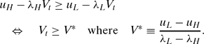
V* is easily interpreted. The numerator is the flow cost of choosing higher performance; the denominator is the effect on the hazard rate of ministerial resignation. The ratio of these terms is the effective cost of reducing resignation risk: Only when his career value exceeds this does the minister find it worthwhile to perform well. To ensure that e † = eL we simply check that a minister's terminal payoff in a failed government is low enough; this is the simple inequality V †<V*.
A government can remain in office despite poor performance so long as it sustains a sufficiently large stock of popular goodwill. An implication is that periods of poor performance sustained by negative expectations may be prolonged. For example, the Brown government limped to electoral defeat in 2011 despite a month by month decrease in opinion polls and amidst consistent concerns about its performance. We have noted in the past that the empirical work of researchers who focus on the length of time that a government survives is related to a concern for government stability that may be misguided; it is perhaps better to focus on the time during which a government performs well (Dewan and Myatt Reference Dewan and Myatt2010). Lemma 1 revealed a maximum length of time τ toward the end of a government's time in office where popularity is declining. Here we can calculate explicitly the (maximum) length of this low-performance era.
In this high-or-low world, this era corresponds to times where a minister's career value satisfies the inequality Vt < V*. To check when this inequality holds, we solve explicitly the differential equation (3) while imposing the boundary condition VT = V †. During the twilight of a government's life (when  , so that et = eL) the solution is straightforwardly obtained:

The first term on the right-hand side is the value of holding a position in an immortal government while delivering low performance. The second term exp [−λL(T−t)] is the probability that the minister survives until the end of the government's lifetime. If this happens, then the low-performance career value is swapped for the terminal payoff V †; this generates the third and final term.
The solution for Vt in (7) has the properties we expect: The value of a minister's career is decreasing in t or, equivalently, increasing in the perceived remaining lifetime T−t. So, moving back through time, Vt grows until eventually it reaches the critical value V*.Footnote 16 Thus, setting  and Vt = V* yields a unique solution for τ, which is reported in Proposition 3. This also determines the size of the maximum buffer of popularity that can be eliminated during the government's decline.
Proposition 3.For the binary-action specification (where each minister chooses between high and low performance) the maximum length of the low-performance era is

The popularity that can be depleted in this time is  .
Recall that x is a critical popularity level: If the government is more popular than this ( ) then there is a unique equilibrium in which the government is immortal.
Some comparative-static predictions that emerge are very natural. Both x and τ are decreasing in uH: Making high performance more attractive shortens the period of declining popularity and so lowers the bar to the unique-immortal-equilibrium regime. Note also that x and τ are both increasing in uL, so that a greater payoff from low-performance lengthens the declining popularity era. However, this is perhaps misleading, because increasing uL while uH is fixed mixes together two effects: It makes it more costly to supply high performance, thereby encouraging lower performance, but at the same time it increases the value of a minister's career, which encourages high performance. To isolate these two effects, it useful to rewrite τ as

Fixing the cost uL−uH and effect λL−λH of heightened performance, τ and x are decreasing in uL. This works through an income effect: Making his career more valuable encourages a minister to work harder to retain his job. The impact of such income effects on politician's incentives has been noted by Besley (Reference Besley2004), and our analysis confirms the robustness of those findings.
A further comparative-static result is that τ and x both fall as the terminal payoff V † grows. Thus, enhancing the value of a surviving minister (perhaps even via the receipt of a “golden handshake” conditional on serving a full term) works in favor of increased performance. This might appear counterintuitive: Increasing postcareer earnings should make maintaining a government career (relatively) less valuable and make ministers more willing to switch. However, the overall benefit of a minister's career, relative to being fired from his position (rather than relative to his career as an ex-minister untainted by scandal) rises, and so the income effect induces higher performance.Footnote 17 The gain in performance may even offset the more obvious costs stemming from a conflict of interest that arise when allowing executive members to accept lucrative postministerial positions. In the United Kingdom, ministers must consult the committee for Standards in Public Life if they accept private sector posts within two years of leaving the government. There has been media pressure to restrict postministerial career earnings; however, our analysis suggests that there may be countervailing implications from such a move.
This discussion refers to the general set of equilibria. However, we may also straightforwardly extend Proposition 3 to the case of Markovian equilibria. For the Markovian case, the performance choice and career value of a minister depend on the current popularity of the government rather than on calendar time.
Corollary (to Proposition 3). For any threshold  , where xis obtained from Proposition 3, there is a Markovian equilibrium. Performance satisfies e(x) = eH for x > x* and e(x) = eL for x < x*. For x < x* (so the government is mortal),

but otherwise, for x > x*, a minister's career value is V(x) = V ‡ = uH/λH.
A value function solution that emerges from this corollary is illustrated in Figure 5.
Markov Value Functions and the Popularity Threshold
Notes. This is value function V(x) for a Markovian equilibrium in a binary-action world. The lower bound for popularity is xL = 0; the terminal payoff for a minister is V † = 0. The other parameter choices are uL = 7, λL = 2, and rL = −1 for the low-performance regime; and uH = 4, λH = 1, and rH = 1 for the high-performance regime. Given that V † = 0, for the “pessimistic” regime where x < x*, the value function (the solid line in the figure) satisfies

This function hits V* at a popularity level of x, which in this case satisfies x = log(7)/2; there is a Markovian equilibrium for any x* below this.

RANDOM SHOCKS AND CRISES OF CONFIDENCE
Thus far we have considered a world in which a government's popularity evolves deterministically as a result of ministers’ action choices, and ministers can anticipate how their careers will progress. A missing ingredient is the element of uncertainty about a government's popularity and survival prospects. Ministers in the United Kingdom's recent Brown administration would of course have reacted with caution to the good news of an early bounce in the opinion polls and government fortunes beginning May 10, 2007. In calculating his career value he would have anticipated that what goes up can come back down, and not always directly as a result of ministers’ actions. In the remainder of the article we consider a more realistic world where uncertainty is present and its presence is understood when ministers choose their actions. We continue with the sharper binary-action specification of the previous section, and we consider (as in the Corollary to Proposition 3) a Markovian equilibrium with a threshold of x*. Here we discuss what happens when popularity equals that threshold.
Suppose that a minister sees that xt = x*, so that the popularity of the government is on a knife's edge between “good” (long-term survival) and “bad” (inevitable decline) worlds, but anticipates a possible shock to the government's popularity. For instance, we can imagine a situation in which the latest macroeconomic statistics (inflation, unemployment, and so on) are about to be announced; such an announcement might contain either good or bad news for a government's popularity. At this point in time a positive shock (for instance, a drop in unemployment) can allow the government to escape up into the good regime, in which case the minister's career is worth V ‡; however, a negative shock (for instance, higher than expected inflation) can push the government's popularity down into the bad regime, in which case ministers career is worth V(x*), where the formula for V(x) is from (10). For the purposes of an informal discussion, suppose that these two shocks are equally likely. If this is so, then the minister's expected career value is (V ‡+V(x*))/2, which is the simple average of the “good news” and “bad news” possibilities. Now, x* is the critical popularity threshold at which the minister's behavior switches from low performance to high performance. Thus, at the threshold a minister should be indifferent between these choices. This is so if and only if his career is worth precisely V* to him. That is,
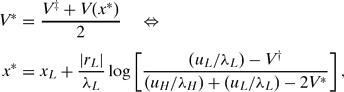
where the solution for x* is obtained after using the formula for V(x*) from (10). Thus the threshold lies at the point where the career valuation V* that prompts higher performance lies halfway between the career values in the optimistic and pessimistic regimes.Footnote 18 The threshold x* illustrated in Figure 5 satisfies this property.Footnote 19
To make this argument rigorous, we revert to a model in which the evolution of popularity is explicitly subject to random events. Setting σ>0, evolving popularity satisfies the stochastic differential equation dxt = r(et) dt+σ dzt. Whereas the drift of popularity (up or down) is determined (via r(et)) by the executive's performance, the Brownian motion term dzt means that unforeseen shocks, policy disasters, and the whims of public opinion can destabilize even the best performing executive; similarly, good luck may help rescue an otherwise doomed administration. We surmise that many governments have been subject to shocks not under their control and that this affects the calculations made by members of the executive about the value of their careers. There is evidence that the public's evaluations do indeed depend on random events—droughts, floods, and (even) shark attacks—that occur during their period of tenure (Achen and Bartels Reference Achen and Bartels2004) and that economic shifts that are plausibly unrelated to an incumbent's performance are nevertheless related to their career prospects (Wolfers Reference Wolfers2007). Our rational expectations model thus seeks to incorporate these factors: A politician anticipates the effect that shocks might have on the government's popularity and so his career value, when choosing his performance.
As before, a minister faces uncertainty because poor individual performance may lead to his own premature demise; this is reflected in the performance-dependent hazard rate λ(e). But now he is also uncertain about his government's longevity. This uncertainty stems from the random shock σ dzt which can push against the established drift of popularity. Even when the government's popularity falls far below the threshold x*, it remains possible that a lucky streak of positive outcomes could lift popularity above the threshold; a minister in a declining government should recognize this possibility. Similarly, a high-performing government enjoying maximum goodwill can always suffer a run of bad luck. In the absence of random events, a single commonly understood barrier separates the worlds of optimism (xt > x*) from those of pessimism (xt < x*); when random events are present then these two worlds may collide.
Turning to our formal analysis, we consider Markovian equilibria in which a minister's career value V(x) and performance choice e(x) both depend solely on the government's current popularity. (We will subsequently confirm that there are no non-Markovian equilibria.) As before, performance is determined by the minister's desire to keep his job, and so satisfies the optimality condition  from (24). The extra step needed for the analysis of a world with random shocks is a careful consideration of a minister's evolving career valuation V(x).
As before, V(x) is increasing in x. However, in contrast to the earlier nonrandom world, V(x) is smoothly and strictly increasing in x; the discontinuity that appears in Figure 5 cannot be present when σ>0, and there cannot be a range of popularities where V(x) is constant. To see why, note that in the nonrandom world V(x) is constant only when V(x) = V ‡ for x > x*; that is, when the government is immortal. Once random events are present, however, there is always a positive probability that a run of bad luck results in the government's defeat. Thus V(x) < V ‡ for all x, and recalling the arguments used previously we can establish that career values must be strictly enhanced by greater popularity. The presence of uncertainty also rules out any discontinuities; the ebb and flow of random events smooth out the transition across any possible discontinuity. Thus, a sharp step up in a minister's career at an arbitrary threshold, as in Figure 5, cannot occur.
We now describe the differential equation that captures the link between popularity and the value of a minister's career. As before, simple accounting ensures that

where it is understood that u and λ both depend on a minister's performance choice, and so on the current state of popularity via the perceived career value V(x). The first and second terms are as before; they represent the flow payoff from holding office and the expected loss from a premature forced resignation. The third and final term is the expected change in a minister's career value owing to the passage of time. When popularity evolves predictably then this is constant. However, here we need to take expectations into account because the minister's career value can be influenced by random events. Adopting a second-order Taylor expansion and taking expectations (in more formal terms, this is the deployment of Itô’s Lemma) we obtain

where it is understood that r depends on aggregate performance and so, via V(x), on the current popularity enjoyed by the government.Footnote 20 Bringing together (12) and (13), the value equation, on the one hand, with that describing the evolution of the career value as popularity ebbs and flows on the other, we obtain

Solving for a Markovian equilibrium boils down to solving for the right solution of this differential equation. Of course, such a second-order differential equation typically has a family of solutions, and so we need to look for two boundary conditions to pin down a unique value function, and so a unique equilibrium.
To obtain the necessary conditions, we consider the value function at its boundaries. The first condition is that VL(0) = V †: Ministers who serve out their term obtain a “golden handshake” worth V † when the government dies with them in post. We condition used this to characterize the solution for V(x) for x < x* when we analyzed a world without random shocks. Here, however, this boundary condition is not enough, because of the second-order term in the differential equation (14). The second condition we need is obtained by looking at what happens when popularity reaches its maximum at xH. The condition we need is V′(xH)=0. This “smooth pasting” condition says that as popularity approaches its upper bound xH it asymptotes; heuristically, this prevents a minister from expecting his career value to crash through its upper bound and so ensures that V(xt) faces a ceiling at V(xH).
With all of the ingredients in place, we are in a position to characterize fully the (unique) Markovian equilibrium. Here we restrict our attention to offering a full solution in a binary-action world. However, the approach we have taken here applies to a wider range of circumstances. With a binary specification (either high or low performance) a threshold x ⋄ separates (much as before) the optimistic high-performance honeymoon world from the pessimistic low-performance waning popularity world. Within each of the two segments of the value function (that is, either side of x ⋄) the parameters u, λ, and r that are present in the differential equation (14) are all constant. When this is so, the equation is linear and so easy to solve. In the Appendix we derive separate solutions and stitch them together at the transition threshold x ⋄.Footnote 21
Proposition 4.Consider a binary-action world in which σ>0. Define:

where UL≡uL/λL, where UH≡uH/λH, and where V*≡(uL−uH)/(λL−λH).
If xH > x*>xL and if σ2is sufficiently small, then there is a unique Markovian equilibrium in which ministers choose high performance if and only if popularity exceeds a unique critical threshold x ⋄satisfying xH > x ⋄ > xL and where  .
When x* falls outside the stated range, then ministers are either unflinchingly optimistic (high performance for all x if x*<xL) or never have sufficient popularity to perform highly (if x*>xH). When xH > x*>xL then we have a unique equilibrium in which performance is high when popularity is above the threshold, and low when it falls below the threshold. When rL = −rH then the solution for x* given in (15) is precisely that given by (11), which followed our earlier heuristic argument.
The unique Markovian equilibrium described thus provides a framework that relates performance, popularity, and a government's longevity. The properties of this equilibria are similar to those described earlier in Proposition 2: A commonly understood barrier separates worlds of optimism (xt > x*) and pessimism (xt < x*). However now we have uniquely defined the barrier between optimism and pessimism and so can provide a one-for-one link between the level of a government's performance and its longevity. The predictions of the model do not depend on the equilibrium analyzed.
THE DYNAMICS OF POPULARITY AND PERFORMANCE
Adding noise to our model not only pins down a unique equilibrium but this dose of realism also allows us to address empirical puzzles so far unexplained in the literature. With noise in its level of popularity the government is subject to the whims of public opinion that are not directly related to its performance. Recent research has shown that the reelection of executives depends on circumstances that are beyond their control. Wolfers (Reference Wolfers2007) analyzed whether voters respond to variation in state economic outcomes that reflect clearly exogenous and easily observed shocks. He found that although voters are able to distinguish local performance from national trends, the reelection rates of U.S. governors are systematically related to national changes in oil prices. This can be seen as evidence of superficial irrationality on behalf of the electorate (see also Achen and Bartels Reference Achen and Bartels2004).
By incorporating these behavioral features—via the noise term in the evolution of government popularity—our rational expectations model provides a channel from these random shocks to the survival of the executive that can plausibly explain patterns in the data. Suppose that the government is indeed punished for events beyond its control so that a random shock can cause the government's popularity to fall. Moreover suppose that the shock (or perhaps a series of shocks) is sufficient to shift perceptions of ministers into the pessimistic waning popularity region that in turn induces low performance. As we have seen, the switch in the expectations of ministers is reinforced by poor performance. This, in turn, increases the likelihood the government will fall. In conclusion, although exogenous shocks such as oil price hikes cannot rationally be attributed to incumbent performance, they can (in a rational expectations framework) affect performance in a way that hastens the government's demise. We note that (some portion of) the estimate of the effects of oil shocks (or flu epidemics, shark attacks, and the like) might be due to variation in performance that results from such shocks.Footnote 22
Although our model is abstract and builds on primitive political forces, namely the rise and fall of a government's popularity, it nevertheless can shed new light on several cases; in particular, those where governments have experienced sharp and sudden crises of confidence. Many governments have been affected by shocks that are unpredicted or implausibly related to their performance in office, before becoming embroiled in scandal and subject to terminal decline. British history offers a very pertinent case of Lord Russell's Whig government that took office during the Irish famine. The devastating effects of this natural disaster were worsened by the lack of action taken by ministers in the Russell government.
More recent cases include governments that have fallen as a result of the financial crisis in 2008. The remarkable fall of Ireland's Fianna Fáil, the dominant party in government for much of its 85-year history, is perhaps most illustrative. Support for the Fianna Fáil government had proved resilient through almost all of the postwar era. In early 2008 its popularity rating stood at a high of 63%. In our parlance this high support operated as a “buffer” that insulated the government against shocks to its popularity. Indeed, this proved to be so. The Fianna Fáil government was affected by several shocks—scandals throughout 2007 and 2008—but its support remained resilient and its majority in the Dail unquestioned. The financial crisis that began in 2008 eventually changed this picture, first denting support before it plummeted. This pattern is reflective of the effects of an unpopular austerity package (imposed at the behest of the International Monetary Fund), but the effect was enhanced by months of scandals, poor communication, and resignations of government ministers. Most commentators believed that by the time of the (unsuccessful) vote of confidence in January 2011 the party had gone beyond the point of no return. Indeed the once dominant party in the Irish political system was reduced to a rump party in the national elections that followed, receiving just 15% of the vote.
A similar story can be told of the Brown government, though it weathered the financial storm relatively well; as we have plotted in Figure 2 a series of shocks affected confidence in the government, pushing it into what we have termed the “zone of pessimism.” After 2008, Brown's exhortations to his party at its annual conference in 2009— “we need to fight; not bow out, not walk away, not give in, not give up, but fight”—were interpreted by many as a last rallying call to a party that had given up the ghost. Indeed such calls did little to generate a boost in performance or avoid a heavy defeat in the election of May 2010.
Our agency model provides an account of these events that is consistent with rational expectations. Once an initial buffer of support is eroded ministers anticipate that further shocks and scandals will push the government into the abyss. With the writing on the wall, performance falters in line with a decrease in the value of a ministerial career. Thus the end of the government becomes a self-fulfilling prophecy.
In obtaining a unique equilibrium, we also enhance the empirical relevance of our model by providing comparative-static predictions. An increase in x* following a parameter change corresponds to an expansion in the size of the zone of pessimism. For instance, notice immediately that x* is decreasing in V †, and so, equivalently, an increase in V † helps to encourage optimism; thus a golden handshake enhances performance and lengthens the average tenure of ministers. The insight here is subtle. An exogenous increase in V † means a relative increase in the payoff associated with a minister having served out his term relative to being forced out of office due to negligence or scandal. This at once makes the government's demise less painful from the minister's perspective, while increasing the relative cost borne should he (alone) be forced out of the administration and the government continues. Our comparative-static analysis tells us that, despite the increase in the postministerial career payoff, the overall effect is to enhance ministerial performance, government popularity, and government's longevity.
The effect of postcareer earnings on political performance has been the subject of investigation. For example, Alesina and Spear (Reference Alesina and Spear1988) highlighted that the last-term effect, commented on earlier, is offset when payments made to a politician subsequent to leaving office are conditional on last-period performance; in their model, valuable payments to a president after leaving office depend on the entire record of policy performance. The difference in our institutional setting—the absence of term limits and the collective nature of the executive—means that such income effects work via different and more subtle channels. Specifically, an increase in V † makes a full service record more desirable from a minister's perspective. This means that ministers increase their performance levels. Responding to their incentives in this way maintains the government in office for longer. An interesting effect is that an increase in the value of a golden handshake delays government termination, and hence the time at which the prize for completing a ministerial term is realized.
Other comparative-static results also follow by inspection. Quite naturally, the threshold x* falls, and so the size of the pessimistic world narrows, as we either increase rH or reduce |rL|. These parameters are the rates at which popularity rises and falls, respectively, in the high-performance and low-performance regimes.
The responses to the flow-payoff and hazard-rate parameters are also straightforward to obtain: x* is increasing in uL and λH, but decreasing in uH and λL. However, it is arguably more useful to think in terms of the baseline parameters in the low-performance world (that is, uL and λL) together with the effect of a shift from high to low performance (that is, the differences uL−uH and λL−λH). The baseline parameters tell us about the intrinsic benefits and risks of ministerial positions, whereas performance-effect parameters tell us about the relative costs and benefits of greater performance. We record our findings as a corollary to Proposition 4.
Corollary.Fixing the performance-effect parameters, the threshold x* is decreasing in the baseline benefit uL of holding office and increasing in the baseline risk λL. Fixing the baseline parameters, x* is increasing in the cost uL−uH of higher performance and decreasing in the influence λL−λHof that performance on resignation risk.
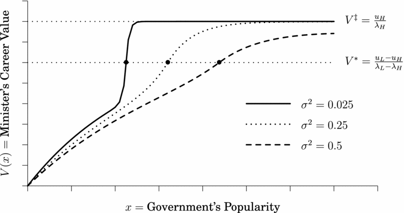
Further predictions are suggested by inspection of Figure 6, which illustrates a minister's equilibrium career value V(x) for different values of the variance term σ2. Note that as noise disappears, then following the heuristic arguments made earlier, V* falls midway between V(x*) and V ‡. (More generally, the location of V* between these two sides of the transition point depends on the relative size of rH and |rL|.) Around the critical threshold even a small increase in popularity can have a large effect on ministerial career values: Once popularity surpasses the threshold, performance is high and small shocks are insufficient to stop ministers from attaining V ‡; similar observations apply below the threshold. As noise increases (a rise in σ) this is no longer so. Any popularity boost that shifts performance (from low to high) faces a good chance of being reversed. So, even when popularity is at its highest level there remains a serious risk that a run of bad luck will bring the administration to its end. The implication is that greater noise reduces ministerial career values (as illustrated in Figure 6) and so acts as a brake on performance. A higher threshold must then be breached before performance switches. Indeed, and following this logic, as σ grows large then high performance can never be attained; in fact, the high-performance region disappears when σ is large.
Value Function and Popularity Threshold with Random Events
Notes. This figure illustrates the value function V(x) and critical popularity threshold arising from the unique equilibrium of a binary-action world with randomly evolving popularity. The parameter choices (xL = 0, xH = 1.5, V † = 0, uL = 7, λL = 2,rL = −1, uH = 4, λH = 1, and rH = 1) match those used in Figure 5. The value function is plotted for three different choices of σ. The bullet points “●” indicate the location of the threshold x ⋄ for these three cases. As σ → 0 the value function converges to the value function in Figure 5.
Our key insight is that policy shocks and disasters are filtered via the three critical ingredients of our model: (i) they affect confidence in the executive's capacity to govern effectively; (ii) they have an impact on perceptions held by government ministers about the security of their tenure and hence the current value of their political careers, and (iii) they affect executive performance, which in turn affects (i) and (ii). Via these mechanisms, a series of good shocks can bolster a government's fortunes and lengthen its tenure, whereas a series of negative shocks can hasten its demise.
Figure 7 reports a single simulation of evolving popularity for the model specification used in earlier figures. Initially, the government begins as a high-performance regime. About halfway through its (realized) term, small negative shocks push popularity to below the threshold level. Subsequently, low performance implies a downward trend until all popularity evaporates. Importantly, if popularity is far above the threshold level then the executive is able to withstand shocks; close to the threshold, however, a small tremor can spark a terminal decline. Although such paths for government popularity are observed in political life, dynamic models in political science that can provide insight to such phenomenon have been, until now, underdeveloped.
Sample Path of Evolving Popularity
Notes. This is a sample path for evolving popularity, generated using a discrete-time approximation to our continuous-time specification. The parameter choices (xL = 0, xH = 1.5, V † = 0, uL = 7, λL = 2,rL = −1, uH = 4, λH = 1, and rH = 1), which match those used in Figures 5 and 6, are supplemented with a variance of σ2 = 0.5. This generates an equilibrium threshold satisfying x*≈0.875. The discrete-time approximation uses a time step of Δt = 0.005.

PERIODIC EVALUATION
Our model captures the interplay between longevity and performance; we hope that our messages (multiple self-fulfilling prophecies, random events allow a unique prediction, and crises of confidence may be sparked by a run of bad news) are robust. However, there are situations to which our messages apply but where our precise model structure relates less well: There are no explicit term-length limits or elections in our model, yet both are present in many settings of interest.
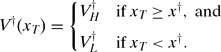
Here we modify our model to consider a government that is subject to periodic evaluation by an electorate or by some other principal. Most components are as before: Each minister chooses performance to balance flow payoff and resignation risk, and the executive's performance determines the evolution of popularity. The difference is that the administration ends at a fixed date T, so the government's lifetime is now exogenous. However, a new endogenous element is the outcome for ministers on the “day of reckoning” when the government's term ends: a minister's terminal payoff V †(xT) is an increasing function of the government's final popularity. According to the form of V †(xT), several applied situations can be captured.
One case of interest is when the government's terminal popularity needs to exceed a critical value x † if it is to serve another term. For instance, x † could be interpreted as the required vote share for the incumbent to enjoy a parliamentary majority. We write V †H for the terminal payoff of a reelected minister; this is the value of an office in a reelected administration. Similarly, we write V †L for the terminal payoff when the government is defeated. Making the natural assumption that V †L<V †H,
A second case of interest is obtained by interpreting the popularity of a government as its probability of reelection on the date of reckoning. This leads to

Simply assuming that V †(xT) is increasing is enough to generate a feedback loop: If the government expects to do well at election time (that is, xT is high) then ministers’ terminal careers will be valuable; this generates higher career values earlier in the government's term, which induces higher performance; and, finally, such higher performance fulfills the expectations of good reelection prospects. Obviously, pessimistic self-fulfilling prophecies are also possible.
Here we limit ourselves to dealing with a specific worked-example specification. We continue with the binary-action specification (so each minister chooses either high or low performance at each moment of time), and we combine this with the threshold-to-win specification from (16) (so that a minister is reelected at time T if xT ≥ x †, but falls with the goverment if xT < x †). We make the assumptions that
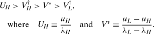
Recall that V* is the career value needed to induce a minister to supply high performance. The inequality V*>V †L means that a minister in a goverment that faces imminent defeat just prior to time T will be unwilling to deliver high performance; the inequality V †H > V* ensures that a popular incumbent executive supplies high performance close to the election date; and the inequality UH > V †H means that a minister would prefer his government to enjoy a infinitely long term of office.
What matters here is whether or not ministers expect the government to continue at time T. If they do, then careers are valuable and ministers choose high performance throughout the government's term. If they do not, then they perform highly only when their careers are sufficiently valuable, which happens only early in the term.
Lemma 2.Consider an environment in which the government is subject to periodic evaluation, and popularity needs to exceed a threshold for the government to continue. If ministers expect reelection ( xT > x †) then they choose high performance throughout. However, if they expect failure ( xT < x †) then there is a unique length of time
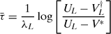
such that ministers choose high performance if and only if  .
There are two types of equilibrium paths for government popularity. First, high performance may be sustained throughout if terminal popularity exceeds xT. Given that popularity increases at rate rH, a lower bound to popularity earlier in the term is needed for this to be an equilibrium: We need xt > x †−rH(T−t) at time t. If this fails for some t, then the government falls at the day of reckoning, which means that performance must tail off. Second, performance may be high (and popularity increasing) prior to  , but low (so that popularity wanes) afterward. For this to be an equilibrium, popularity must fall below x † by the end. So, for instance, we need xt < x †−rL(T−t) for
 . Putting these observations together, we may characterize the set of rational-expectations equilibria (see Figure 8 for illustrations).
Equilibrium Popularity Paths in the Day-of-Reckoning Model
Notes. This figure illustrates possible equilibrium paths for popularity. The upper broken line is xt (see Proposition 5). Above it, the government always survives reelection; the top solid arrow shows such an equilibrium path, beginning from the “○” symbol. The lower broken line is  (see again Proposition 5). Below, the government is always defeated; again, a solid arrow shows the equilibrium path. Between the two broken lines, there are both “good” and “bad” equilibria. For instance, starting from the remaining “○” symbol there is a unique equilibrium path with growing popularity until time
 . However, for
 there are two possibilities: popularity continues to grow in an optimistic equilibrium, ending above x † and so justifying the optimism; or, popularity falls in a pessimistic equilibrium, ends below x †, and the government falls.

Proposition 5.Define the upper and lower popularity thresholds  as

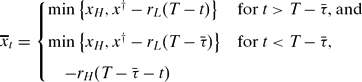
In a rational-expectations equilibrium, beginning from time t with popularity xt : (i) if xt > xt then performance is high, popularity rises, and the government is reelected; (ii) if  , then performance is high and popularity rises for
 , but performance is low and popularity falls afterward and the government is defeated at time T ; and (iii) for intermediate cases
 both (i) and (ii) are equilibria.
In contrast to our main model, notice that there are situations in which a “bad” equilibrium is inevitable; if the government's popularity is too low (if  , or below the lower broken line in Figure 8) then there is simply too little time for it to recover before the day of reckoning. Such an equilibrium also has interesting dynamic properties: Popularity is potentially non-monotonic, because ministers deliver high performance only earlier in the government's term, when their careers are sufficiently valuable.
NONEXISTENCE OF A MARKOVIAN EQUILIBRIUM
Proposition 4 characterizes a unique Markovian equilibrium. However, we still need to consider the possibility of non-Markovian equilibria in which ministers’ career values and performance choices depend on some aspect of history other than the government's current popularity. In the absence of random events, Proposition 1 describes such an equilibrium, in which popularity first rises and then falls. We have expressed misgivings about that non-monotonic equilibrium, and we hinted that such an equilibrium may not be robust to the presence of random shocks. Our next result confirms that the shocks to popularity eliminate non-Markovian equilibria.
Proposition 6.Under the conditions of Proposition 4 there are no non-Markovian equilibria, and hence the equilibrium described in Proposition 4 is unique.
Here we limit ourselves to a brief sketch of why this result is true. In any non-Markovian equilibrium the career value of a minister must be at least as good as his career value in the worst possible Markovian equilibrium. (The worst possible equilibrium is Markovian simply because it involves ministers adopting the most pessimistic expectations irrespective of history.) Similarly, the career value must be no better than his career value in the best possible Markovian equilibrium. However, as we have shown, when random shocks are present there is a unique Markovian equilibrium. This ties down Markovian career values and so uniquely defines the equilibrium career value (and behavior) of ministers.
RELATED LITERATURE
In addition to our main contribution in providing micro-foundations for a reciprocal causal relationship between tenure and performance, and to our understanding of the dynamics of government fortunes over time (following our introductory remarks), we highlight three other related areas: (i) the relationship between agency and performance (ii) the determinants of government survival, and (iii) the political and economic analysis of common-resource-pool problems.
Our article contributes to a broad literature that considers the effect of agency on performance. At a basic level, government performance depends on the qualities of office holders and their incentives, and so a large literature has addressed aspects of adverse selection and moral hazard (Barro Reference Barro1973; Fearon Reference Fearon, Przeworski, Stokes and Manin1999; Ferejohn Reference Ferejohn1986). Dynamic models that include both adverse selection and moral hazard have also been developed (Banks and Sundaram Reference Banks, Sundaram, Barnett, Hinich and Schofield1993; Reference Banks and Sundaram1998). A more recent contribution that corresponds to our focus on politicians’ time horizons and their performance is that of Ashworth (Reference Ashworth2005). He analyzed the retention of politicians whose abilities are unobserved by an electorate who instead observe a politician's record of constituency service. In his equilibrium, “veteran” politicians provide lower levels of service though this does not have a negative effect on their reelection probability.
Studies of agency relations in parliamentary settings (Berlinski, Dewan, and Dowding Reference Berlinski, Dewan and Dowding2010; Dewan and Dowding Reference Dewan and Dowding2005; Huber and Martinez-Gallardo Reference Huber and Martinez-Gallardo2008) have related ministerial turnover to the arrival of new information to a leader. In contrast Dewan and Myatt (Reference Dewan and Myatt2007b; Reference Dewan and Myatt2010) and Indridason and Kam (Reference Indridason and Kam2008) assessed how the executive leader provides incentives via the firing rule. Here we do not consider firing rules, but instead focus on our main new contributions: an analysis of the team dynamics of government performance, a focus on strategic complementarities that arise, and a novel resolution to a thorny equilibrium-selection problem.
Our focus on the collective fate of the executive relates our work to the literature on government survival (Laver Reference Laver2003 offers a review). We have developed a new set of modeling techniques to analyze the dynamic process of government duration and thereby build micro-foundations for the “events” theory of government dissolution (Browne, Frendreis, and Gleiber Reference Browne, Frendreis and Gleiber1984; Reference Browne, Frendreis and Gleiber1986). This theory relates a government's tenure to shocks that are beyond executive control. In earlier theoretical models (Diermeier and Stevenson Reference Diermeier and Stevenson2000; Lupia and Strøm Reference Lupia and Strøm1995), random shocks perturb the key parameters of a defined government formation game, providing incentives for an early dissolution of government. Our model does not rely on such bargaining dynamics. Instead we describe more general factors that relate to a wider set of cases including, though not limited to, multiparty parliamentary regimes.
Moving beyond the specific application of our model, our analysis yields insights into a collective action problem. Popularity is a stock of goodwill that helps a government to survive; it is a common-pool resource. Dynamic models of the common-pool-resource problem have been developed in economics by Tornell and Velasco (Reference Tornell and Velasco1992) among others. In an important and provocative contribution Kremer and Morcom (Reference Kremer and Morcom2000) modeled the harvesting of open-access resources. When such resources are storable (the example of elephant-sourced ivory motivated their article) expectations over future prices determine current prices and so current depletion. If complete exhaustion of the resource is expected then future prices are higher; this bids up current prices; which in turn drives up current exploitation, and so fulfills the prophecy of extinction. In contrast, there is also a sustainable equilibrium in which the resource survives, and so prices and harvesting are both low. Related ideas have developed elsewhere in economics. For instance, Rowat and Dutta (Reference Rowat and Dutta2007; Reference Rowat and Dutta2011) analyzed commons exploitation in the presence of capital markets and found multiple equilibria: Either commons exploitation is low and the commons regenerates in steady state, or exploiters expect exhaustion and so rush to grab the remaining resource before it runs out, hence causing the exhaustion. Where these economic models fail, however, is in resolving the problem of multiple equilibria. In our model the addition of random events that buffet popularity provides unique predictions. Our analysis carries over to different aspects of politics involving common-pool resources: It could be applied fruitfully to assess the effect of institutional rules on fiscal outcomes as analyzed by Hallerberg and Marier (Reference Hallerberg and Marier2004), for example. Indeed whereas Bejar, Mukherjee, and Moore (Reference Bejar, Mukherjee and Moore2011) viewed the common-resource-pool problem and short time horizons as rival explanations for poor performance (they assessed fiscal ill discipline) in parliamentary democracies, our framework incorporates both elements. Finally, our model may prove useful for studying nongovernmental organizations where similar incentives are at play. An obvious example is team sports where a string of bad luck or a series of lucky breaks can have dramatic effects on subsequent performance and success. Thus our solution opens new possibilities for dynamic analysis of common-resource problems in economics, political science, and beyond.
CONCLUDING REMARKS
We set out to explore the determinants of a government's performance and longevity. Although much empirical work is guided by insights from essentially static models, we have provided an integrated account of the dynamic interplay between a government's survival and performance that sheds light on the reciprocal relationship between these variables. In a simple model, multiple rational-expectations equilibria can arise: In one, high expectations of government survival fuel good performance that sustains government popularity and secures an indefinite term of office; but in other equilibria, ministers coordinate around a pessimistic outlook on government fortunes, ministerial career values fall, and corresponding low effort ensures a drop in popularity and a finitely lived government. Augmenting the model to allow for stochastic shocks to government popularity, however, allows for a unique prediction. Then self-fulfilling pessimistic and optimistic expectations can be overcome by a string of good or bad fortune, and a unique threshold separates the worlds of pessimism and optimism: Ministers perform well (and so popularity rises in expectation) if and only if popularity exceeds this critical threshold.
Our model makes several contributions to an understanding of dynamic government processes. First, we show that insights from the literature on fixed term lengths and performance travel beyond cases of U.S. federal states to parliamentary democracies where term length is endogenous to performance. Second, we show that institutions generating longer time horizons can have a positive effect on performance that in turn bolsters a government's survival prospects. Third, our dynamic model provides a rigorous and coherent framework for understanding episodes of crises of confidence that involve the rapid collapse of government performance and of survival prospects that occur when a sequence of negative shocks pushes popularity below a threshold. Fourth, our model provides a rational-expectations explanation for the relationship between random shocks and government turnover that analysts of public opinion often attribute to superficial irrationality by the electorate.
More generally, our model offers a methodological contribution toward the study of dynamic collective action problems. Our application helps the understanding of executive politics and the role played by politicians’ time horizons. Here we have studied how the time horizons of ministers affect their incentives, in a situation where they cannot outlive the government they serve and where the government is subject to either ongoing or periodic evaluation. Similar insights could emerge when considering other institutions such as political parties or family dynasties.
APPENDIX: OMITTED PROOFS
Monotonicity of Ministerial Career Values. As the end of government draws near, a minister's career becomes less valuable and so performance falls. To verify that this is so, we combine (3) and (4). Doing so, Vit satisfies

The right-hand side is increasing in Vit. Hence, if the right-hand side is positive (respectively, negative) for some t, then Vit is increasing (respectively, decreasing) in t, which means that it must be increasing (respectively, decreasing) for all larger t; this observation, once developed, establishes that Vit is monotonic in t. To check that Vit is decreasing, it is sufficient to compare Vit at t = Ti (so that Vit = V †) and in the limit as Ti−t → ∞, so that Vit → V ‡. By assumption V ‡ > V †, and so a minister's career value does fall over time; optimally chosen performance is monotonically related to career value and so performance must also decline over time. ■
Lemma 1 and Proposition 1. These results follow from arguments given in the text. ■
Proof of Proposition 2. Recall that at time t each minister chooses performance e(xt), has a career value V(xt), and expects the government to last until T = t+τ(xt).
Some properties of a Markovian equilibrium are immediate. The executive's remaining lifetime τ(x) must be (at least weakly) increasing in popularity: Starting from some higher level x′>x, popularity must decline through the lower level x before the government term ends and so τ(x′) ≥ τ(x). The government may be perceived as immortal, and so there is a “popularity threshold” x*∈[xL, xH] such that τ(x)=∞ for all x > x*, but τ(x) is finite when x*>x > xL. If popularity falls below the threshold then it must strictly fall over time; if it remained constant then (because behavior is Markovian) it would remain constant forever, sustaining the government evermore. In sum, τ(·) is a strictly increasing function below x*, but becomes infinite (and so constant) above the popularity threshold.
The properties of τ(x) carry over to a minister's career value: V(x) is a strictly increasing function for x < x*, and (because of the perceived immortality of the administration) satisfies V(x) = V ‡ for x > x*. When x < x* we can calculate V(x) by assessing the value of a minister's career in the pessimistic equilibrium described in Proposition 1. Such a pessimistic path can be consistent with rational expectations only when  , which in turn implies that the popularity threshold must satisfy
 . In the pessimistic zone, it is also straightforward to characterize how a minister's career value changes as a function of changes in popularity. The differential equation (3) can be modified appropriately for this environment to yield

which again stems from straightforward accounting. Within (23), the performance term e(x) is obtained from the optimality condition (4), so that

To obtain a complete solution for V(x) for x < x* we need only a condition provided by the terminal-payoff condition at the expiration of the government's term: V(xL) = V †. ■
Proof of Proposition 3. For the binary action case eit = eL and λ(eit)=λL so long as  . Hence, for such times the differential equation (22) reduces to
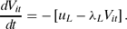
It is straightforward to confirm that the solution for Vit given in (7) satisfies this equation and also satisfies Vit when t = Ti. To find τ we simply set Ti−t = τ and Vit = V*. Doing so and solving for τ yields (8) in the statement of the proposition. Over the final τ periods of the government's life, confidence depletes at rate |rL|, which generates the final claim of the proposition. ■
Proof of Proposition 4. V(x) satisfies the second-order differential equation (14),

where in general the terms u, λ, and r all depend on performance e(x) where  . Naturally, without further structure we are unable to describe an explicit general solution to this differential equation. However, for the binary-action case the terms u, λ, and r are all locally independent of x away from the threshold x*. Hence, for x≠x* the differential equation (26) is linear, and so is easily solved. When x > x*, this general solution is
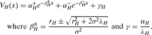
and where the α±H coefficients remain to be determined. Similarly, for x < x*,
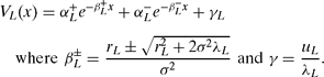
These two components to the value function solution must join smoothly at the critical confidence threshold x*. Moreover, at the threshold the career value of a minister must make him indifferent between high and low performance. Hence

The overall solution must also satisfy the two boundary conditions discussed in the text. Using the notation introduced here, these conditions are

Equations (29) and (30) yield five equations that determine five unknowns: the free parameters α±L and α±H from the value function solutions and the confidence threshold x*.
It is straightforward to solve for the four free parameters α±L and α±H in terms of x* by considering separately the two segments of the value function. Consider the pessimistic segment. The conditions VL(xL) = V † and VL(x*) = V* are
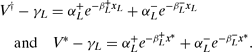
These equations are linear in α+L and α−L, and solve straightforwardly:


Note that  , and so
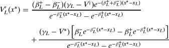
Now consider the optimistic segment. The conditions VH(x*) and V′H(xH)=0 are
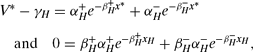
and these solve to give us


We can plug these solutions into  and obtain

So far we have obtained solutions for the value function in both the pessimistic and optimistic worlds as a function of the critical confidence threshold x*. These solutions satisfy the relevant boundary conditions and meet at VL(x*) = VH(x*) = V*. The one remaining condition is that V′L(x*) = V′H(x*), so that the two different parts of the value function meet smoothly at the confidence threshold. We can use this condition to find x*, by equating the expressions in (34) and (38).
Clearly, we cannot obtain a general explicit solution for x*. However, when noise is low (so that σ2 is small) the expressions for V′H(x*) and V′L(x*) simplify dramatically. To proceed, first let us note the limiting values of the β±L and β±H parameters as σ2 → 0:

(The limiting properties of β−H and β+L are obtained via an application of l'Hôpital's rule.) Inspecting the expression (38) for V′H(x*), for x*<xH notice that  while
 remains finite, and so the former term in both the numerator and denominator of V′H(x*) dominates when σ2 is small. This means that, for small σ2, we have V′H(x*)≈β+H(γH−V*). More formally,

Similarly, for V′L(x*) in (34) and for x*>xL terms involving  dominate. Taking limits, we find that
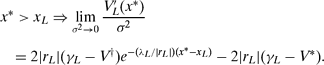
Equating the expressions in (40) and (41) yields the solution for x* given in (15). The comparative-static results given in the text and the corollary are obtained by differentiation of x* with respect to the parameters of interest. ■
Proof of Lemma 2. If the government survives at time T, then the career value of a minister is at least V †H throughout. V †H > V* and so he delivers high performance. If the government falls at T, then the career value continuously falls to V †L as T approaches. Therefore in the twilight of the government's term, a minister delivers low performance. Recycling the earlier analysis, Vt = UL−exp (−λL(T−t))(UL−V †L). This is below V*, so generating low performance, if and only  as stated. ■
Proof of Proposition 5. Performance is high and popularity grows at times  . For
 performance is high and popularity is growing if ministers expect xT > x †. Of course, starting from popularity xt at time t, we need to check that there is enough time for popularity to grow to above its final target. This is possible if and only if
 . Remaining elements of the proposition are obtained in a similar way. ■
Proof of Proposition 6. Here we sketch the argument for why this proposition is true. For any equilibrium, what matters is the career value of a minister. (That career value can be used to compute a minister's performance.) Let us write ht for the history of the government other than its popularity at time t; thus ht contains everything other than the fundamental state of the government's situation. We write a minister's equilibrium career value as V(xt, ht) in a possibly non-Markovian equilibrium.
Now consider the worst possible equilibrium career value. Starting from any time and any popularity, the set of continuation equilibria depend only on xt. (Our model is not formally game-theoretic, but if it were then each time t would begin a subgame, where that subgame would depend only on xt.) Let us pick the worst one; that is, the one with lowest career value and so the lowest performance. It is straightforward to confirm that this procedure constructs a Markovian equilibrium, and we write VW(xt) for the career value generated. We can go through the same procedure and find the best possible equilibrium career value for a minister: For each point in time and each popularity, we abandon nonfundamental history and pick the highest continuation career value. We write VB(xt) the corresponding best career value beginning from xt.
Doing all this, the equilibrium career value V(xt, ht) for a minister in a non-Markovian equilibrium must satisfy VB(xt) ≥ V(xt, ht) ≥ VW(xt); it is better than the worst Markovian equilibrium and worse than the best Markovian equilibrium. However, when random shocks are present, there is a unique Markovian equilibrium with a unique career value V(x), and so VB(xt) = VW(xt) = V(xt). Thus, V(xt, ht) = V(xt). ■
 . This assumption ensures that the career value of a minister declines as the expected life of his government shortens.
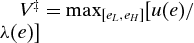 .
 the value of T allows just enough time to eliminate the initial stock; it satisfies x 0 = xL−∫T0r(et) dt. It is straightforward to confirm that this equation has a unique solution
 . When
 the length
 of the high-performance regime must be just enough for popularity to grow from its initial value to the peak; formally,
 .





Comments
No Comments have been published for this article.