


1. Introduction
In this paper we derive central limit theorems (CLTs) for mean and variogram estimators for a field (Xi)i∈ℤd, defined by
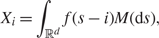 \begin{equation}X_i=\int_{\mathbb{R}^d}f(s-i)M(\!\text d s),\end{equation}
where M is an infinitely divisible, independently scattered random measure on ℝd and f is some kernel function.
Lévy-based models as defined in (1.1) provide a flexible modelling framework that has recently been used in a range of modelling contexts, including modelling of turbulent flows, growth processes, Cox point processes, and brain imaging data [Reference Barndorff-Nielsen and Schmiegel3], [Reference Hellmund, Prokešová and Jensen7], [Reference Jónsdóttir, Schmiegel and Jensen9], [Reference Jónsdóttir, Rønn-Nielsen, Mouridsen and Jensen10].
Due to the tractability of Lévy-based models, it has been possible to derive tail asymptotics for the supremum of such a field as well as asymptotics of excursion sets of the field. The case where M is a convolution equivalent measure is considered in [Reference Rønn-Nielsen and Jensen12] and [Reference Rønn-Nielsen and Jensen13]. Results for random measures with regularly varying tails have been derived in [Reference Rosiński and Samorodnitsky15], and refined in [Reference Adler, Samorodnitsky and Taylor1] and [Reference Adler, Samorodnitsky and Taylor2].
In [Reference El Machkouri, Volný and Wu4], CLTs are proved for a stationary random field (Xi)i∈ℤd, discretely defined by
 \begin{equation}X_i=u(M_{s+i}\colon s\in \mathbb{Z}^d),\end{equation}
where (Mi)i∈ℤd are independent and identically distributed (i.i.d.) random variables and u is a measurable function. In contrast, our setup involves a random measure defined on ℝd. However, if we discretize the integral in (1.1) then our model is of the form (1.2) with u a linear function and the random variables Mi having an infinitely divisible distribution. Note that if this type of model is going to hold for finer and finer resolution, then the common distribution of the random variables Mi has to be infinitely divisible.
For a random field defined by (1.1), we prove in the present paper CLTs for
 $$S_\Gamma=\sum_{i\in\Gamma}X_i \quad \mathrm{and}\quad
T_\Gamma(h)=\sum_{i\in\Gamma}(X_i-X_{i+h})^2,$$
where h ∈ℤd and Γ is a finite subset of ℤd with the number of elements increasing to infinity. We show, under mild regularity conditions, that both S Γ and T Γ (h) are asymptotically normally distributed and give explicit expressions for the asymptotic variances. It turns out that the asymptotic variance of T Γ (h) is equal to an approximate variance, earlier derived in [Reference Rønn-Nielsen, Sporring and Jensen14]. In the latter paper, the approximate variance was used in the assessment of the precision of a section spacing estimator in electron microscopy. More details are given in Section 5.
If we discretize the integral in (1.1), both S Γ and T Γ(h) take the form
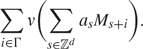 \begin{equation}\sum_{i\in\Gamma}v\biggl(\sum_{s\in\mathbb{Z}^d}a_s M_{s+i}\biggr).
\end{equation}
Here, v(x) = x and as = f (s) for S Γ, while v(x) = x 2 and as = f (s) − f (s − h) for T Γ(h). In [Reference El Machkouri, Volný and Wu4], CLTs for random variables of the form (1.3) are discussed. In particular, a CLT for S Γ is derived which is a discrete analogue of the CLT we obtain. For second-order properties, El Machkouri et al. [Reference El Machkouri, Volný and Wu4] considered
 $$\sum_{i\in\Gamma}X_i X_{i+h},$$
but did not deal explicitly with the case where the mean of the field is unknown, as is done in this paper.
The present paper is organised as follows. In Section 2 we define the random field (1.1) and state the main result. In Section 3 we provide the proofs. An important tool in the proofs will be a CLT (Theorem 3.1) for mn-dependent fields proved in [Reference Heinrich5]. In Section 4 we discuss the case where the kernel function is isotropic, while the results are used for the estimation of sample spacing in Section 5. Cumulant formulae and a proof of a corollary to Ottaviani’s inequality are deferred to Appendices A and B.
2. Preliminaries and the main result
Consider an independently scattered random measure M on ℝd. Then, for a sequence of disjoint sets (An)n∈ℕ ⊆ ℝd in  $\cal{B}({ {\mathbb R}}^d)$, the random variables (M(An))n∈ℕ are independent and satisfy M(∪ An) = Σ M(An). Assume furthermore that M(A) is infinitely divisible for all
 $A\in\cal{B}({ {\mathbb R}}^d)$. Then M is called a Lévy basis; see [Reference Barndorff-Nielsen and Schmiegel3] and the references therein.
For a random variable X, let κX(λ) denote its cumulant function log  ${\rm {\mathbb E}}(\text e^{\text i\lambda X})$. We shall assume that the Lévy basis is stationary and isotropic such that, for
 $A\in\cal{B}({ {\mathbb R}}^d)$, the variable M(A) has a Lévy–Khintchine representation given by
 $$\kappa_{M(A)}(\lambda)=\text i \lambda am_d(A)-\frac{1}{2}\lambda^2\theta
m_d(A)+\int_{A\times{\rm {\mathbb R}}}(\text e^{\text i\lambda u}-1-\text i\lambda
u1_{[-1,1]}(u))F(\text d s,\text d u),$$
where md is the Lebesgue measure on 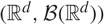 $({{\mathbb R}^d},\cal{B}({ {\mathbb R}}^d))$, a ∈ ℝ, θ ≥ 0, and F is a measure on
 $\cal{B}({ {\mathbb R}}^d\times {\rm {\mathbb R}})$ of the form
 $$F(A\times B)=m_d(A)\rho(B),$$
such that ρ is a Lévy measure.
In the following, we let M′ be a so-called spot variable, i.e. M′ is a random variable with the distribution of M(A) for  $A\in\mathcal{B}({ {\mathbb R}}^d)$ with md(A) = 1. We will assume that the Lévy measure ρ satisfies
 $$\int_{[-1,1]}z^2\,\rho(\text d z)\lt \infty\quad\text{and}\quad
\int_{[-1,1]^c}|z|\rho(\text d z)\lt \infty.$$
The first assumption is needed for ρ to be a Lévy measure. The second assumption is equivalent to  ${\rm {\mathbb E}}|M'|\lt \infty$ (see [Reference Sato16, Theorem 25.3]). Now assume that f : ℝd → [0, ∞) is a bounded kernel function satisfying
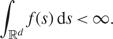 \begin{equation}\int_{ {\mathbb R}^d}f(s)\text d s\lt \infty.
\end{equation}
Let ℤd be the grid integer numbers in ℝd. We consider the family of random variables (Xi)i∈ℤd defined by
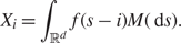 \begin{equation}X_i=\int_{ {\mathbb R}^d}f(s-i)M(\text d s).
\end{equation}
See [Reference Rajput and Rosiński11, Theorem 2.7] for existence of the integrals, where their conditions (i)–(iii) can be easily verified under the given assumptions on M and f. The field is stationary, and if furthermore f has the form f (s) = g(||s||), where || · ||; is Euclidean norm, it will be isotropic. This special case is studied in Section 4.
We will be interested in estimating the mean and the variogram of the field. We have
 $$\mu={\rm {\mathbb E}} X_0={\rm {\mathbb E}}(M')\int_{ {\mathbb R}^d}f(s)\text d s,$$
and, for h ∈ ℤd,
 $$\gamma(h)={\rm {\mathbb E}}(X_{0}-X_{h})^2={\rm var}(M')\int_{\ {\mathbb R}^d}(\,f(s)-f(s-h))^2\text d s,$$
where identities from Appendix A have been applied. Note that, due to stationarity,  $\mu={\rm {\mathbb E}} X_i$ and
 $\gamma(h)={\rm {\mathbb E}}(X_{i}-X_{i+h})^2$ for all i ∈ ℤd. For Γ a finite subset of ℤd, we define
 $$S_\Gamma=\sum_{i\in\Gamma} X_i,$$
and, for h ∈ ℤd,
 $$T_\Gamma(h)=\sum_{i\in\Gamma}(X_i-X_{i+h})^2.$$
Unbiased estimators for μ and γ (h) are respectively obtained as
 $$\widehat{\mu}=\frac{1}{|\Gamma|}S_\Gamma,\qquad
\widehat{\gamma(h)}=\frac{1}{|\Gamma|}T_\Gamma,$$
Where |Γ| denotes the number of elements in Γ. The main result gives asymptotic normality of these estimators for |Γ| going to infinity.
Theorem 2.1. Let (Γn)n≥1 be a sequence of finite subsets of ℤd, and assume that |Γn| goes to infinity and |∂Γn|/|Γn| goes to 0. Let
 $$\sigma_S^2={\rm var}(M')\sum_{i\in { {\mathbb Z}^d}}\int_{ {\mathbb R}^d}f(s)f(s-i)\text d s.$$
If  $\sigma_S^2\lt \infty$ then
 $$\frac{S_{\Gamma_n}-|\Gamma_n|\mu}{\sqrt{|\Gamma_n|}}\underrightarrow{\rm D}\mathcal{N}
(0,\sigma^2_S).$$
If furthermore 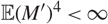 ${\rm {\mathbb E}}(M')^4\lt \infty$ then
 $$\frac{T_{\Gamma_n}(h)-|\Gamma_n|\gamma(h)}{\sqrt{|\Gamma_n|}}
\underrightarrow{\rm D}\mathcal{N}(0,\sigma^2_T),$$
where
 $$\sigma_T^2=\sum_{j\in{ {\mathbb Z}^d}}\left[\kappa_4(M')\int_{ {\mathbb R}^d}
g(s)^2g(s-j)^2\text d s+2{\rm var}(M')^2\left(\int_{ {\mathbb R}^d} g(s)g(s-j)\text d
s\right)^2\right]\lt \infty,$$
κ 4(M′) is the fourth cumulant of M′, and g(s) = f (s) − f (s − h).
It should be noted that the assumptions of the theorem,
 $$|\Gamma_n|\to\infty\quad\text{and}\quad \frac{|\partial
\Gamma_n|}{|\Gamma_n|}\to 0,$$
are equivalent to the (less intuitive, but more computationally convenient) properties
 $$|\Gamma_n|\to\infty\quad\text{and}\quad
\frac{|(\Gamma_n-j)\cap \Gamma_n|}{|\Gamma_n|}\to 1$$
for all j ∈ ℤd, where Γ + j denotes the translation of Γ in direction j ∈ ℤd, i.e.
 $$\Gamma+j=\{i+j\mid i\in\Gamma\}.$$
3. Proofs
An important tool in the proof of our main result, Theorem 2.1, is a CLT for mn-dependent random fields that may be found in [Reference Heinrich5, Theorem 2]. Results on bounds for the error in CLTs for random fields generated by functions of independent random variables can be found in [Reference Heinrich6] together with a description of the history of CLTs for that type of random field. Theorem 2 of [Reference Heinrich5] is also used in the proofs of the CLTs, derived in [Reference El Machkouri, Volný and Wu4]. However, our proof of the CLT for S Γ is simpler and takes advantage of the linearity of the Lévy-based model (1.1), while our proof of the CLT for T Γ(h) follows a different route than the one adopted in [Reference El Machkouri, Volný and Wu4] for the second-order property Σi∈Γ XiXi +h.
Recall that a random field (Zi)i∈ℤd is said to be mn-dependent if, for any A, B⊂ℤd with |A|, |B| < ∞ and inf{ ||a − b|| : a ∈ A, b ∈ B} > mn ∈, (Za)a∈A and (Zb)b∈B are independent. The CLT for mn-dependent fields is here stated as follows.
Theorem 3.1. Let (Γn)n≥1 be a sequence of finite subsets of ℤd with |Γn| → ∞ as n → ∞, and let (mn)n≥1 be a sequence of positive integers. For each n ≥ 1, let {Un(j), j ∈ ℤd} be an mn-dependent random field with  ${\rm {\mathbb E}} U_n(j)=0$ for all j ∈ ℤd. Assume that
 ${\rm {\mathbb E}}(\!\sum_{j\in\Gamma_n}U_n(j))^2\to\sigma^2$ as n → ∞ with σ 2 < ∞. Then Σj∈Γn Un(j) converges in distribution to a Gaussian random variable with mean zero and variance σ 2 if there exists a finite constant c > 0 such that, for any n ≥ 1,
 $$\sum_{j\in\Gamma_n}{\rm {\mathbb E}} U_n(\,j)^2\leq c,$$
and, for any ε > 0, it holds that limn→∞ Ln(ε) = 0, where
 $$L_n(\varepsilon)=m_n^{2d}\sum_{j\in\Gamma_n}{\rm {\mathbb E}}\left(U_n(\,j)^2{\bf 1}{\{|U_n(\,j)|\geq\varepsilon m_n^{-2d}\}}\right)\!.$$
Proof of Theorem 2.1 for S Γn. Let (mn)n≥1 be a sequence of integers increasing to infinity. The choice of the sequence will be specified below.
For i ∈ ℤd and n ∈ ℕ, let Cn(i) be the ball in ℝd with center in i and radius mn/3. Let
 $$\overline{X}^n_i=\int_{C_n(i)}f(s-i)M(\text d s);$$
furthermore, let  $\mu_n={\rm {\mathbb E}}(\overline{X}_0^n)={\rm {\mathbb E}}(M')\int_{C_n(0)}f(s)\text d s$ and
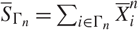 $\overline{S}_{\Gamma_n}=\sum_{i\in\Gamma_n}\overline{X}_i^n$. The proof will be divided into two steps. The first step is to show that
 \begin{equation}\lim_{n\to\infty}\frac{\| S_{\Gamma_n}-|\Gamma_n|\mu-(\overline{S}_{\Gamma_n}-|\Gamma_n|\mu_n)\|_2}{\sqrt{|\Gamma_n|}}=0\,.
\end{equation}
The second step is to show, using Theorem 3.1, that with an appropriately chosen sequence (mn)n≥1 we have
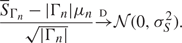 \begin{equation}\frac{\overline{S}_{\Gamma_n}-|\Gamma_n|\mu_n}{\sqrt{|\Gamma_n|}}
{\underrightarrow{\rm D}}
\mathcal{N}(0,\sigma_S^2).
\end{equation}
To prove (3.1), we find, using the results in Appendix A,
 \begin{align}{\frac{\|S_{\Gamma_n}-|\Gamma_n|\mu-(\overline{S}_{\Gamma_n}-|\Gamma_n|\mu_n)\|_2^2}{|\Gamma_n|}\\ \quad\quad\quad =\frac{1}{|\Gamma_n|}{\rm {\mathbb E}}\left[\left(\sum_{i\in\Gamma_n}\left[\int_{C_n(i)^c}f(s-i)M(\text d s)-{\rm {\mathbb E}}(M^\prime)\int_{C_n(i)^c}f(s-i)\text d s\right]\right)^2\right]\\ \quad\quad\quad =\frac{1}{|\Gamma_n|}\sum_{i\in\Gamma_n}\sum_{j\in\Gamma_n}{\rm Cov}\left[\int_{C_n(i)^c}f(s-i)M(\text d s),\int_{C_n(\,j)^c}f(s-j)\,M(\text ds)\right]\\ \quad\quad\quad =\frac{{\rm var}(M^\prime)}{|\Gamma_n|}\sum_{i\in\Gamma_n}\sum_{j\in\Gamma_n}\int_{C_n(i)^c\cap C_n(\,j)^c}f(s-i)f(s-j)\text d s\\ \quad\quad\quad \leq \frac{{\rm var}(M^\prime)}{|\Gamma_n|}\sum_{i\in\Gamma_n}\sum_{j\in{ {\mathbb Z}^d}}\int_{C_n(i)^c\cap C_n(\,j)^c}f(s-i)f(s-j)\text d s\\ \quad\quad\quad ={\rm var}(M^\prime)\sum_{j\in{ {\mathbb Z}^d}}\int_{C_n(0)^c\cap C_n(\,j)^c}f(s)f(s-j)\text d s\\ \quad\quad\quad \to 0,}\end{align}
where the convergence is a result of dominated convergence, since
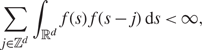 \begin{equation}\sum_{j\in{ {\mathbb Z}^d}}\int_{ {\mathbb R}^d} f(s)\,f(s-j)\text d s \lt \infty,
\end{equation}
and Cn(0)c ∩ Cn(j)c → ∅ as n → ∞.
In order to prove (3.2), for n ∈ ℕ and j ∈ ℤd, define
 $$U_n(j)=\frac{\overline{X}_j^n-\mu_n}{\sqrt{|\Gamma_n|}}$$
such that
 $$\sum_{j\in\Gamma_n}U_n(j)=\frac{\overline{S}_{\Gamma_n}-|\Gamma_n|\mu_n}{\sqrt{|\Gamma_n|}}.$$
Then, clearly (Un(j))j∈ℤd is mn-dependent with  ${\rm {\mathbb E}} U_n(j)=0$ for all n ≥ 1 and j ∈ ℤd. Furthermore (cf. Appendix A),
 \begin{align*}{{\rm {\mathbb E}}\left[\left(\sum_{i\in\Gamma_n}U_n(i)\right)^2\right] =\frac{1}{|\Gamma_n|} \sum_{i\in\Gamma_n}\sum_{j\in\Gamma_n}{\rm Cov}\left[\int_{C_n(i)}f(s-i)M(\text d s), \int_{C_n(\,j)}f(s-j)M(\text d s)\right] \\ \quad\quad\quad\quad\quad\quad\quad\quad\space =\frac{{\rm var}(M^\prime)}{|\Gamma_n|}\sum_{i\in\Gamma_n}\sum_{j\in\Gamma_n} \int_{C_n(i)\cap C_n(\,j)}f(s-i)f(s-j)\text d s \\ \quad\quad\quad\quad\quad\quad\quad\quad\space ={\rm var}(M^\prime)\sum_{j\in{ {\mathbb Z}^d}}\frac{|(\Gamma_{n}-j)\cap \Gamma_n|}{|\Gamma_n|} \int_{C_n(0)\cap C_n(\,j)}f(s)f(s-j)\text d s \\ \quad\quad\quad\quad\quad\quad\quad\quad\space \to {\rm var}(M^\prime)\sum_{j\in{ {\mathbb Z}^d}}\int_{ {\mathbb R}^d} f(s)f(s-j)\text d s }\end{align*}
as n → ∞, by dominated convergence. Here, we have used the facts that (3.3) is fulfilled, |(Γn − j) ∩ Γn|/|Γn| → 1 for all j, and Cn(0) ∩ Cn(j) → ℝ d as n → ∞. Furthermore, we find (cf. Appendix A) that
 $$\sum_{i\in\Gamma_n}{\rm {\mathbb E}}[U_n(i)^2]={\rm var}(\overline{X}_0^n)={\rm var}(M')
\int_{C_n(0)}f(s)^2\text d s\leq {\rm var}(M')\int_{ {\mathbb R}^d} f(s)^2\text d s \lt \infty.$$
Now let
 $$Y=\sup_{n\geq 1}|\overline{X}_0^n-\mu_n|.$$
Note that the sequence  ${(\bar X_0^n)_{n \ge 1}}$ has independent increments and that
 \begin{equation}
\sup_{n\geq 1}{\rm {\mathbb E}}\big[(\overline{X}_0^n-\mu_n)^2\big]=\sup_{n\geq
1}{\rm var}(M')\int_{C_n(0)}f(s)^2\,\text d s\leq {\rm var}(M')\int_{ {\mathbb R}^d} f(s)^2\text d
s\lt \infty.
\end{equation}
Then  ${\rm {\mathbb E}} Y^2\lt \infty$, due to Corollary B.1. Furthermore,
 \begin{align*}
L_n(\varepsilon)&=m_n^{2d}\sum_{j\in\Gamma_n}{\rm {\mathbb E}}\left[U_n^2(\,j){bf 1}{\{|U_n(j)|
\geq \varepsilon m_n^{-2d}\}}\right]
\\
&=m_n^{2d}{\rm {\mathbb E}}\left[(\overline{X}_0^n-\mu_n)^2{bf 1}{\{|\overline{X}_0^n-\mu_n|
\geq \varepsilon\sqrt{|\Gamma_n|} m_n^{-2d}\}}\right]
\\
&\leq m_n^{2d}{\rm {\mathbb E}}\left[Y^2{bf 1}{\{Y\geq \varepsilon\sqrt{|\Gamma_n|} m_n^{-2d}\}}
\right]
\\
&=m_n^{2d}{\rm {\mathbb E}}\left[Y^2{bf 1}{\{Y\geq \varepsilon\sqrt{|\Gamma_n|} m_n^{-2d},\,
Y\leq |\Gamma_n|^{1/4}\}}\right]+m_n^{2d}{\rm {\mathbb E}}\left[Y^2 {bf 1}{\{Y\geq
\varepsilon\sqrt{|\Gamma_n|} m_n^{-2d},\,Y\gt |\Gamma_n|^{1/4}\}}\right]
\\
&\leq m_n^{2d}\sqrt{|\Gamma_n|}{\rm {\mathbb P}}\left[Y\geq \varepsilon\sqrt{|\Gamma_n|}
m_n^{-2d}\right]+m_n^{2d}{\rm {\mathbb E}}\left[Y^2{bf 1}{\{Y\gt |\Gamma_n|^{1/4}\}}\right]
\\
&\leq \frac{m_n^{6d}}{\varepsilon^2\sqrt{|\Gamma_n|}\,}{\rm {\mathbb E}} Y^2+m_n^{2d}
\psi(|\Gamma_n|^{1/4}),
\end{align*}
where  $\psi(x)={\rm {\mathbb E}}(Y^2{bf 1}{\{Y\geq x\}})$. Note that ψ (x) → 0 as x → ∞. With ⌊·⌋ denoting the integer part, now choose the sequence (mn)n≥1 as mn = ⌊| Γn|1/(24d) ⌋ if ψ(| Γn|1/4) = 0 and
 $$m_n=\min\{\lfloor\psi(|\Gamma_n|^{1/4})^{-{1}/{(4d)}}
\rfloor,\lfloor|\Gamma_n|^{{1}/{(24d)}}\rfloor\}$$
otherwise. With this choice, it is seen that Ln(ε) → 0 as n → ∞. Thus, from Theorem 3.1, we have
 $$\frac{\overline{S}_{\Gamma_n}-|\Gamma_n|\mu_n}{\sqrt{|\Gamma_n|}}\underrightarrow{\rm D}
\mathcal{N}(0,\sigma^2_S)\,.$$
Combining this with (3.1) yields the desired result.
In the proof of Theorem 2.1 for T Γn(h), we need the following lemma, the proof of which follows from straightforward calculations, using the fact that f is bounded and nonnegative.
Lemma 3.1. For h ∈ ℤd, let
 $$g(s)=f(s)-f(s-h),\qquad s\in {{\mathbb R}^d}.$$
Then, for s ∈ ℝd and j ∈ ℤd,
 \begin{align*}
|g(s)g(s-j)|\leq v_j(s),\quad\quad
g(s)^2g(s-j)^2\leq Cv_j(s),
\end{align*}
where
 $$v_j(s)=f(s)\,f(s-j)+f(s)\,f(s-h-j)+f(s-h)\,f(s-j)+f(s-h)\,f(s-h-j)$$
and C < ∞ is an appropriately chosen constant. If
 $$\sum_{j\in{ {\mathbb Z}^d}}\int_{ {\mathbb R}^d}f(s)\,f(s-j)\text d s\lt \infty$$
then
 $$\sum_{j\in{ {\mathbb Z}^d}}\int_{ {\mathbb R}^d}v_j(s)\,\text d s\lt \infty\quad\text{and}\quad
\sum_{j\in{ {\mathbb Z}^d}}\left(\int_{ {\mathbb R}^d}v_j(s)\text d s\right)^2\lt \infty.$$
Proof of Theorem 2.1 for T Γn(h). First note that it follows from Lemma 3.1 that  $\sigma_S^2\lt \infty$ and
 ${\rm {\mathbb E}}[(M')^4]\lt \infty$ implies that
 $\sigma_T^2\lt \infty$.
For ease of notation, we shall now consider the field (Yi)i∈ℤd, where Yi = Xi − Xi +h. Then, for all i ∈ ℤd,  ${\rm {\mathbb E}} Y_i=0$ and
 $${Y_i} = \mathop \smallint \nolimits_{\rm{\mathbb R}}^d (f(s - i) - f(s - i - h))M({\rm{d}}s) = \mathop \smallint \nolimits_{\rm{\mathbb R}}^d g(s - i)M({\rm{ds}}),$$
where g(s) = f (s) − f (s − h) as previously. Let (mn)n≥1 be (another) sequence of integers increasing to infinity. Let Cn(i) and  $\overline{X}_i^n$ be defined as in the proof of Theorem 2.1 for S Γn. Let
 $$\bar Y_i^n = \bar X_i^n - \bar X_{i + h}^n = \mathop \smallint \nolimits_{{{\rm{\mathbb R}}^d}}^{} {g_n}(s - i)M({\rm{ds}}),$$
where gn(s) = 1Cn(0)(s)f (s) − 1Cn(h)(s)f (s − h). Then gn(s) → g(s) for all s ∈ ℝd. Note that  ${\rm {\mathbb E}} \overline{Y}_i^n=0$ = 0 and, furthermore, let
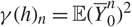 $\gamma(h)_n={\rm {\mathbb E}} (\overline{Y}_0^n)^2$ Also, define
 $\overline{T}_{\Gamma_n}(h)=\sum_{i\in\Gamma_n}(\overline{Y}^n_i)^2$.
As for S Γn, the first step will be to show that
 \begin{equation}\lim_{n\to\infty}\frac{\| T_{\Gamma_n}(h)-|\Gamma_n|\gamma(h)-(\overline{T}_{\Gamma_n}(h)-|\Gamma_n|\gamma(h)_n)\|_2}{\sqrt{|\Gamma_n|}}=0.
\end{equation}
The second step is to show, using Theorem 3.1, that with an appropriately chosen sequence (mn)n≥1 we have
 \begin{equation}\frac{\overline{T}_{\Gamma_n}(h)-|\Gamma_n|\gamma(h)_n}{\sqrt{|\Gamma_n|}}
{\xrightarrow{\text{\upshape\sc d}}}
\mathcal{N}(0,\sigma_T^2).
\end{equation}
To prove (3.4), we find that
 \begin{align} \frac{\| T_{\Gamma_n}(h)-|\Gamma_n|\gamma(h)-(\overline{T}_{\Gamma_n}(h)
-|\Gamma_n|\gamma(h)_n)\|_2^2}{|\Gamma_n|}\nonumber
\\
\quad\quad=\frac{1}{|\Gamma_n|}{\rm {\mathbb E}}\left[\left(\sum_{i\in\Gamma_n}\left[Y_i^2-{\rm {\mathbb E}}
Y_i^2
-((\overline{Y}_i^n)^2-{\rm {\mathbb E}}(\overline{Y}_i^n)^2)\right]\right)^2\right]\nonumber
\\
\quad\quad=\frac{1}{|\Gamma_n|}\sum_{i,j\in\Gamma_n}{\rm {\mathbb E}}[(Y_i^2-{\rm {\mathbb E}} Y_i^2)(Y_j^2
-{\rm {\mathbb E}} Y_j^2)]\nonumber
\\
\quad\quad+\frac{1}{|\Gamma_n|}\sum_{i,j\in\Gamma_n}
{\rm {\mathbb E}}[((\overline{Y}_i^n)^2-{\rm {\mathbb E}} (\overline{Y}_i^n)^2)
((\overline{Y}_j^n)^2-{\rm {\mathbb E}} (\overline{Y}_j^n)^2)]\nonumber
\\
\quad\quad-2\frac{1}{|\Gamma_n|}\sum_{i,j\in\Gamma_n} {\rm {\mathbb E}}[(Y_i^2-{\rm {\mathbb E}}
Y_i^2)((\overline{Y}_j^n)^2-{\rm {\mathbb E}} (\overline{Y}_j^n)^2)].
\end{align}
We will show convergence of the three terms in (3.6) separately. Using the calculation formulae from Appendix A, the first term equals
 \begin{align}{{1 \over {|{\Gamma _n}|}} \sum\limits_{i,j \in {\Gamma _n}} {\left[ {{\kappa _4}({M^\prime })\int_{{^d}} g {{(s - i)}^2}g{{(s - j)}^2}{\rm{ds + 2var}}{{({{\rm{M}}^\prime })}^{\rm{2}}}{{\left( {\int_{{^{\rm{d}}}} {\rm{g}} ({\rm{s - i}}){\rm{g}}({\rm{s - j}}){\rm{ds}}} \right)}^{\rm{2}}}} \right]} \\ = \sum\limits_{j \in {^d}} {{{|{\Gamma _n} \cap ({\Gamma _n} - j)|} \over {|{\Gamma _n}|}}} \\ \quad\times \left[ {{\kappa _4}({M^\prime })\int_{{^d}} g {{(s)}^2}g{{(s - j)}^2}{\rm{ds + 2var}}{{({{\rm{M}}^\prime })}^{\rm{2}}}{{\left( {\int_{{^{\rm{d}}}} {\rm{g}} ({\rm{s}}){\rm{g}}({\rm{s - j}}){\rm{ds}}} \right)}^{\rm{2}}}} \right].}\end{align}
By dominated convergence, this converges to  $\sigma_T^2$, using the facts that
 $\sigma_T^2$ is finite and that all terms in
 $\sigma_T^2$ are nonnegative. The second term in (3.6) equals
 \begin{align*} \sum_{j\in}{ {\mathbb Z}^d}\frac{|\Gamma_n\cap(\Gamma_n-j)|}{|\Gamma_n|}\\\times\left[\kappa_4(M^\prime)\int_{ {\mathbb R}^d} g_n(s)^2g_n(s-j)^2\text d s+2{\rm var}(M^\prime)^2\left(\int_{ {\mathbb R}^d} g_n(s)g_n(s-j)\text d s\right)^2\right].
\end{align*}
By dominated convergence and Lemma 3.1, applied to gn instead of g, but keeping the upper bound as vj(s), this also converges to  $\sigma_T^2$. Similarly, the third term of (3.6) converges to
 $-2\sigma_T^2$, and we have the desired result in (3.4).
Now, for n ∈ ℕ and j ∈ ℤd, let
 $$V_n(j)=\frac{(\overline{Y}_j^n)^2-\gamma(h)_n}{\sqrt{|\Gamma_n|}}.$$
We want to show that
 $$\sum_{j\in\Gamma_n}V_n(\,j) {\xrightarrow{\text{\upshape\sc d}}}
\mathcal{N}(0,\sigma_T^2)$$
using Theorem 3.1. Then, by construction,  ${\rm {\mathbb E}} V_n(j)=0$ for all n ≥ 1 and j ∈ ℤd, and, for n such that mn/3 > ||h||, the field (Vn(j))j∈ℤ d is mn-dependent. Furthermore,
 \begin{align*}
{\rm {\mathbb E}}\left[\left(\sum_{i\in\Gamma_n}V_n(i)\right)^2\right]&=
\frac{1}{|\Gamma_n|}{\rm {\mathbb E}}\left[\left(\sum_{i\in\Gamma_n}
\left[(\overline{Y}_i^n)^2-{\rm {\mathbb E}}(\overline{Y}_i^n)^2\right]\right)^2\right]
\\
&=\frac{1}{|\Gamma_n|}\sum_{i,j\in\Gamma_n}{\rm {\mathbb E}} [((\overline{Y}_i^n)^2-{\rm {\mathbb E}}
(\overline{Y}_i^n)^2) ((\overline{Y}_j^n)^2-{\rm {\mathbb E}} (\overline{Y}_j^n)^2)],
\end{align*}
which equals the second term of (\ref{fml:3parts}) and therefore has limit
$\sigma_T^2$. Additionally, using the results in Appendix~\ref{app:cumulant},
\begin{align*}
which equals the second term of (3.6) and therefore has limit  $\sigma_T^2$. Additionally, using the results in Appendix A,
 \begin{align*}
\sum_{i\in\Gamma_n}{\rm {\mathbb E}}[V_n(i)^2]&={\rm {\mathbb E}}[[(\overline{Y}_0^n)^2
-{\rm {\mathbb E}}(\overline{Y}_0^n)^2]^2]
\\
&=\kappa_4(M')\left(\int_{ {\mathbb R}^d} g_n(s)^4\,\text d s\right)+2{\rm var}(M')^2
\left(\int_{ {\mathbb R}^d} g_n(s)^2\,\text d s\right)^2
\\
&\leq\kappa_4(M')\left(\int_{ {\mathbb R}^d} v_0(s)^2\,\text d s\right)+2{\rm var}(M')^2
\left(\int_{ {\mathbb R}^d} v_0(s)\,\text d s\right)^2
\\
&\lt \infty
\end{align*}
with v 0 as defined in Lemma 3.1. Now let
 $$Z=(\sup_{n\geq 1}|\overline{X}_0^n|+\sup_{n\geq 1}|\overline{X}_h^n|)^2+C,$$
where
 $$C=2{\rm var}(M')\int_{ {\mathbb R}^d}f(s)^2\,\text d s.$$
Using the results in Appendix A, we find that 0≤ γ (h)n ≤ C for all n ≥ 1. Also, note that the sequence  ${(\bar X_0^n)_{n \ge 1}}$ has independent increments and that, for k = 1, 2, 3, 4 (cf. Appendix A),
 $$\sup_{n\geq 1}\kappa_k\big(\overline{X}_0^n\big)= \sup_{n\geq
1}\kappa_k(M')\int_{C_n(0)}f(s)^k\,\text d s\leq \kappa_k(M')\int_{ {\mathbb R}^d}
f(s)^k\,\text d s\lt \infty.$$
Thus,  $\sup_{n\geq 1}{\rm {\mathbb E}}(\overline{X}_0^n)^4\lt \infty$ also. By stationarity,
 $\sup_{n\geq 1}{\rm {\mathbb E}}(\overline{X}_h^n)^4\lt \infty$ also, and, thus,
 ${\rm {\mathbb E}} Z^2\lt \infty$, due to Corollary B.1. Then
 \begin{align*}
L_n(\varepsilon) =m_n^{2d}\sum_{j\in\Gamma_n}{\rm {\mathbb E}}\left[V_n^2(j){bf 1}{\{|V_n(j)|\geq
\varepsilon m_n^{-2d}\}}\right]
\\
=m_n^{2d}{\rm {\mathbb E}}\left[\Big((\overline{X}_0^n-\overline{X}_h^n)^2-\gamma(h)_n\Big)^2{bf 1}{\{|(\overline{X}_0^n-\overline{X}_h^n)^2-\gamma(h)_n|\geq
\varepsilon\sqrt{|\Gamma_n|} m_n^{-2d}\}}\right]
\\
\leq m_n^{2d}{\rm {\mathbb E}}\left[Z^2{bf 1}{\{Z\geq \varepsilon\sqrt{|\Gamma_n|}
m_n^{-2d}\}}\right].
\end{align*}
Now, it follows that Ln(ε) → 0 by choosing (mn)n≥1 as in the proof of Theorem 2.1 for S Γn. Thus, we can conclude from Theorem 3.1 that
 $$\frac{\overline{T}_{\Gamma_n}-|\Gamma_n|\gamma(h)_n}{\sqrt{|\Gamma_n|}}
\underrightarrow{\rm D}\mathcal{N}(0,\sigma^2_T)\,,$$
and combining this with (3.4) gives the desired convergence.
4. Isotropic model
We make the assumption that the observations in the field have the form
 \begin{equation}X_i=\int_{ {\mathbb R}^d}f(\|s-i\|)M(\text d s)
\end{equation}
for i ∈ ℤd, where f : [0, ∞) → [0, ∞) satisfies
 $$\int_{ {\mathbb R}^d}f(\|s\|)\,\text d s\lt \infty.$$
This is equivalent to assuming that f (s) in (2.2) depends only on s through ||s||. With this assumption, the field is isotropic, so
 $${\rm {\mathbb E}}(X_i-X_j)^2=\gamma(\|i-j\|)$$
for a variogram function γ : [0, ∞) → [0, ∞). Estimation of  $\mu={\rm {\mathbb E}} X_0$ and the corresponding asymptotic properties are unchanged, compared to the more general framework in Section 2. Also, estimation of γ (||h||) for h ∈ ℤdcan be carried out as before, and the asymptotic results are still valid. However, we can improve the variogram estimator by taking into account the fact that γ (||h||) depends only on ||h||. For this, we introduce
 $$T'_\Gamma(d_0)=\frac{1}{|h(d_0)|}\sum_{i\in\Gamma} \sum_{h\in
h(d_0)}(X_i-X_{i+h})^2,$$
where Γ is a finite subset of ℤd, d 0 > 0, and h(d 0) = {h ∈ ℤd : ||h||= d 0}.
Theorem 4.1. Let (Γn)n≥1 be a sequence of finite subsets of ℤd,and assume that |Γn| goes to infinity and |∂Γn|/|Γn| goes to 0. If
 $$\sum_{i\in {{\mathbb Z}^d}}\int_{{\mathbb R}^d}f(\|s\|)\,f(\|s-i\|)\,\text d s\lt \infty.$$
and 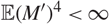 ${\rm {\mathbb E}}(M')^4\lt \infty$, then
 $$\frac{T'_{\Gamma_n}(d_0)-|\Gamma_n|\gamma(d_0)}{\sqrt{|\Gamma_n|}}
\underrightarrow{\rm D}\mathcal{N}(0,\sigma^2_{T'}),$$
where
 \begin{align*}{\sigma_{T^\prime}^2 =\frac{1}{|h(d_0)|^2}\sum_{j\in{ \mathbb Z}^d}\sum_{h,h^\prime\in
h(d_0)}\left[\kappa_4(M^\prime)\int_{ {\mathbb R}^d} g_h(s)^2g_{h^\prime}(s-j)^2\,\text d s
\\ +2{\rm var}(M^\prime)^2\left(\int_{ {\mathbb R}^d} g_h(s)g_{h^\prime}(s-j)\,\text d
s\right)^2\right]\\ < \infty}\end{align*}
and gh(s) = f (||s||) − f (||s − h||).
The proof of Theorem 4.1 follows exactly the same lines as the second part of the proof of Theorem 2.1. Additional notation is only needed to take care of the extra summation in the definition of  $T'_{\Gamma}$.
5. Estimation of sample spacing
Assume that d = 3 and consider the isotropic case again. Let the random field (Xt)t∈ℝ3 be defined as
 $$X_t=\int_{\rm {\mathbb R}^3}f(\|s-t\|)M(\text d s).$$
Suppose that the field is only observed in grid points within two parallel planes with an unknown distance that we want to estimate. Due to the isotropy, we can without loss of generality assume that observations are made in the two planes
 $${\rm {\mathbb Z}}^2=\{(z_1,z_2,0)\colon z_1,z_2\in{\rm {\mathbb Z}}\}$$
and
 $${\rm {\mathbb Z}}^2+h_0=\{(z_1,z_2,d_0)\colon z_1,z_2\in{\rm {\mathbb Z}}\},$$
where h 0 = (0, 0, d 0). The aim is then to estimate d 0. Note that ℤ2 + h 0 ⊂ ℤ3 only if d 0 ∈ ℤ, which is not assumed. The idea will be to estimate γ (d 0), the variogram evaluated in d 0, based only on pairs (i, i + h 0), where i ∈ ℤ2 and I + h 0 ∈ ℤ2 + h 0. For a finite subset Γ ⊂ ℤ2 we can estimate γ (d 0) by 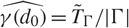 $\widehat{\gamma(d_0)}={\tilde{T}_\Gamma}/{|\Gamma|}$ where
 $$\tilde{T}_{\Gamma}=\sum_{i\in\Gamma}(X_i-X_{i+h_0})^2.$$
Assuming that the variogram function d ↦ γ (d) is known and strictly increasing, an estimator for d 0 is obtained by
 $$\hat{d_0}=\gamma^{-1}(\widehat{\gamma(d_0)}).$$
This estimator is studied in [Reference Rønn-Nielsen, Sporring and Jensen14], where an expression for the variance of T̃Γis derived. Furthermore, an approximate expression for the variance of d̂ 0 is found using a Taylor approximation.
In the following theorem we give the asymptotic normality of T̃Γ. In fact, apart from the scaling, the asymptotic variance is equal to the approximation to the variance suggested in [Reference Rønn-Nielsen, Sporring and Jensen14].
A result showing asymptotic normality of T̃Γ can directly be translated into asymptotic confidence intervals for d̂ 0. If d ↦ γ (d) is also assumed to be differentiable, asymptotic normality of d̂ 0 is easily derived using the delta method.
Theorem 5.1. Let (Γn)n≥1 be a sequence of finite subsets of ℤ2, and assume that |Γn| goes to infinity and that |∂Γn|/|Γn| → 0 for all j ∈ ℤ2 Assume further that 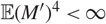 ${\rm {\mathbb E}}(M')^4\lt \infty$ and
 $$\sum_{i\in {\rm {\mathbb Z}^2}}\int_{\rm {\mathbb R}^3}f(\|s\|)\,f(\|s-i\|)\,\text d s\lt \infty.$$
Then
 $$\frac{\tilde{T}_{\Gamma_n}-|\Gamma_n|\gamma(d_0)}{\sqrt{|\Gamma_n|}}
\underrightarrow{\rm D}\mathcal{N}(0,\sigma^2_{\tilde{T}}),$$
where
 $$\sigma_{\tilde{T}}^2=\sum_{j\in{\rm {\mathbb Z}}^2}\left[\kappa_4(M')\int_{ {\mathbb R}^d}
g(s)^2g(s-j)^2\,\text d s+2{\rm var}(M')^2\left(\int_{ {\mathbb R}^d} g(s)g(s-j)\,\text d
s\right)^2\right]\lt \infty$$
and g(s) = f (||s||) − f (||s − h 0 ||).
Above ∂Γn denotes the boundary of Γn as a subset of ℤ2. The proof of Theorem 5.1 is almost identical to the proof of Theorem 2.1, but with ℤd replaced by ℤ2 as the index set for the observations.
Appendix A. Cumulant formulas
For two variables Y 1 and Y 2 of the form (2.2),
 $$Y_1=\int_{ {\mathbb R}^d}f_1(s)M(\text d s),\quad\quad Y_2=\int_{ {\mathbb R}^d}f_2(s)M(\text d s),$$
with kernels f 1 and f 2 satisfying (2.1), the joint cumulant function is given as
 $$\log{\rm {\mathbb E}}\left({\rm e}{\text i(\lambda_1Y_1+\lambda_2Y_2)}\right)
=\int_{ {\mathbb R}^d}\log{\rm {\mathbb E}}\left({\rm e}{\text i(\lambda_1f_1(s)+\lambda_2\,f_2(s))M'}\right)\,\text d
s;$$
see [Reference Hellmund, Prokešová and Jensen7] for details. Assuming that 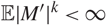 ${\rm {\mathbb E}}|M'|^k\lt \infty$ and differentiating k times with respect to λ 1 gives
 $$\kappa_k(Y_1)=\kappa_k(M')\int_{ {\mathbb R}^d} f_1(s)^k\,\text d s,$$
where κk(X) denotes the kth cumulant of the variable X. Similarly, if 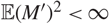 ${\rm {\mathbb E}}(M')^2\lt \infty$, we find that
 $${\rm Cov}(Y_1,Y_2)={\rm var}(M')\int_{ {\mathbb R}^d} f_1(s)f_2(s)\,\text d s.$$
If, furthermore,  ${\rm {\mathbb E}} Y_1={\rm {\mathbb E}} Y_2=0$ and
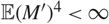 ${\rm {\mathbb E}}(M')^4\lt \infty$, it holds that
 \begin{align*}
&{\rm {\mathbb E}}\big((Y_1^2-{\rm {\mathbb E}} Y_1^2)(Y_2^2-{\rm {\mathbb E}} Y_2^2)\big)
\\
&\quad \quad =\kappa_4(M')\left(\int_{ {\mathbb R}^d} f_1(s)^2f_2(s)^2\,\text d s\right)
+2{\rm var}(M')^2\left(\int_{ {\mathbb R}^d} f_1(s)f_2(s)\,\text d s\right)^2.
\end{align*}
Appendix B. Corollary to Ottaviani’s inequality
In this appendix (Xn)n≥1 will denote a sequence of random variables. Let
 $$S_n=X_1+\cdots+X_n\quad\text{and}\quad M_n=\max_{1\leq k\leq n}|S_k|\,.$$
We will use the following version of Ottaviani’s inequality, see [Reference Hoffmann–Jørgensen8, Section 6.24].
Theorem B.1. Let (Xn)n≥1 be a sequence of independent random variables. Then
 $${\rm {\mathbb P}}(M_n\gt x+y)\cdot \min_{1\leq k\leq n}{\rm {\mathbb P}}(|S_n-S_k|\leq y)\leq {\rm {\mathbb P}}(|S_n|\lt x)$$
for all x, y ∈ ℝ
Corollary B.1. Let (Xn)n≥1 be a sequence of independent random variables. Then, for all p ≥ 1,  $\sup_{n\geq 1}{\rm {\mathbb E}}|S_n|^p\lt \infty$ if and only if
 ${\rm {\mathbb E}} M^p\lt \infty$ where M = supn≥1 Mn.
Note that the corollary can be shown for 0 < p < 1 as well. However, in the present paper we only need the result for p = 2, 4.
Proof of Corollary B.1. First note that it is easy to show directly that  ${\rm {\mathbb E}} M^p\lt \infty$ implies that
 $\sup_{n\geq 1}{\rm {\mathbb E}}|S_n|^p\lt \infty$ The opposite statement follows from monotone convergence, if we can show that, for all n ≥ 1,
 \begin{equation}{\rm {\mathbb E}} M_n^p\leq C \max_{1\leq k\leq n}{\rm {\mathbb E}}|S_k|^p
\end{equation}
for a finite constant C that depends only on p. By assumption,  $\sup_{n\geq 1}{\rm {\mathbb E}}|S_n|^p\lt \infty$ and, therefore,
 $$m=\max_{1\leq k\leq n}{\rm {\mathbb E}}|S_k|^p\lt \infty.$$
Let τ = (2p+1m)1/p. Then, by Markov’s inequality, we have, for 1 ≤ k ≤ n,
 $${\rm {\mathbb P}}(|S_n-S_k|\gt \tau)\leq \frac{{\rm {\mathbb E}}(|S_n-S_k|^p)}{\tau^p}\leq
2^{p}\frac{{\rm {\mathbb E}}|S_n|^p+{\rm {\mathbb E}}|S_k|^p}{\tau^p}\leq \frac{1}{2},$$
where the inequality |x + y|p ≤ 2p(|x|p + |y|p) has been applied. It follows that  $\min_{1\leq k\leq n}{\rm {\mathbb P}}(|S_n-S_k|\leq \tau)\geq \frac{1}{2}$, so, by Theorem B.1,
 $${\rm {\mathbb P}}(M_n\gt x)={\rm {\mathbb P}}(M_n\gt (x-\tau)+\tau)\leq 2 {\rm {\mathbb P}}(|S_n|+\tau\gt x).$$
Integrating both sides with respect to pxp −1 dx gives
 \begin{equation*}
{\rm {\mathbb E}} M_n^p\leq 2{\rm {\mathbb E}}\big((|S_n|+\tau)\,^p\big)\leq
2^{p+1}{\rm {\mathbb E}}(|S_n|^p+\tau^p)\leq 2^{p+1}(1+2^{p+1})m.
\end{equation*}
Acknowledgement
This work was supported by the Centre for Stochastic Geometry and Advanced Bioimaging, funded by the Villum Foundation.


