1 Introduction
A rigid surface imposes two boundary conditions on a Newtonian fluid – a normal or kinematic boundary condition (which can be derived from mass conservation) and a tangential boundary condition based on (indirect) empirical evidence (see Reynolds Reference Reynolds1886; Batchelor Reference Batchelor1967; Lauga, Brenner & Stone Reference Lauga, Brenner, Stone, Tropea, Yarin and Foss2007). In most problems, the kinematic boundary condition reduces to the relative velocity normal to the wall being zero. There are a number of important practical cases where a through-surface flow is either deliberately introduced because it has a beneficial effect or is a consequence of other processes present. These examples include:
-
(i) Cooling turbine blades. The thermodynamic efficiency of combustion is usually increased by raising the temperature of the reaction. To cope with raised temperatures, the surface properties of turbine blades are modified by coating them with a ceramic (Goward Reference Goward1998) or by introducing a flow through surface holes near the leading edge of the blades (Bogard & Thole Reference Bogard and Thole2006). The through-surface flow serves two purposes – first the air cools the blades by passing through their internal structure (Iacovides & Launder Reference Iacovides and Launder1995), and second, the flow introduced at the leading edge displaces both the momentum and thermal boundary layer away from the blade surface reducing the rate of heat transfer. There is also evidence that introducing a blow flow near to the tip of the turbine blade reduces the pressure drop by altering the flow near the tip gap.
-
(ii) Controlling the forces on a rigid body. Applying suction to various parts of a lifting surface of an aerofoil can be used to increase lift by preventing flow separation and stall (see Malavard Reference Malavard1984). Likewise, applying a blowing flow can be used to inject high momentum air to prevent separation. In many cases the flow is directed with a tangential component parallel to the body surface (Nishino & Shariff Reference Nishino and Shariff2012), either through a slot or holes.
-
(iii) Phase change. The evaporation of a fuel droplet leads to it shrinking in time which generates a change in the volume of the dispersed phase and an associated through-surface flux (Crowe Reference Crowe1976). The current trend is for direct injection internal combustion engines where the fuel is injected at pressure, over a short period of time (Zhao, Harrington & Lai Reference Zhao, Harrington and Lai2002). The fuel droplets are typically sufficiently small that their characteristic Reynolds number is smaller than
 $50$
. Likewise, the condensation of vapour bubbles generated by boiling a liquid leads to a relative flow towards the bubble surface, but since this relative speed is proportional to the ratio of vapour to fluid density, this dynamical influence is negligible compared to the influence of changes in topology or vortex shedding (Eames Reference Eames2010).

In examples (i) and (ii), the through-surface flow is usually applied over a portion of the surface of a body surface. The focus in this paper is on the influence of a through-surface flow applied uniformly over the whole of the surface of a bluff body, specifically focussing on a cylinder and sphere, as this serves as a natural starting point to understand the general influence of a through-surface flow applied to portions of a rigid body. Specifically we consider the flow past a rigid surface with an outward flow
 $U_{b}$
, normal to the surface. The flow is characterised by a dimensionless blow velocity
 ${\it\Lambda}=U_{b}/U_{\infty }$
(to use the terminology of the combustion literature); for suction
 ${\it\Lambda}<0$
and for blowing
 ${\it\Lambda}>0$
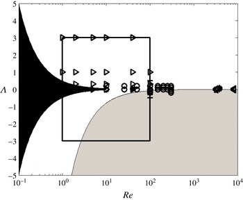
. As a way of identifying gaps in the previous studies, a scatter plot of the parameter range which has been analysed to date is shown in figure 1. The first observation is that the effect of strong sucking flows has not been analysed in great detail analytically or numerically, although there were some excellent experimental studies in the 1950s on cylinders. As we shall see, this is because the boundary layer is extremely thin for
 ${\it\Lambda}<-1$
and the size of the computational domain has a significant and anticipated effect on the force calculation, especially for two-dimensional flows. The second observation from the literature review is that the unsteady and transient component of the flow and forces has not been analysed although this is essential for understanding the progression to steady state. These two gaps form the basis of this paper.
Scatter plot showing a summary of the research on blowing/sucking flow past a cylinder and sphere. The symbols correspond to ○ (Bagchi Reference Bagchi2007, sphere, numerics),
 $+$
(Ling & Fang Reference Ling and Fang2002, cylinder, numerics), ◃ (Fransson, Koniecznyb & Alfredsson Reference Fransson, Koniecznyb and Alfredsson2004, cylinder, experiments), ▹ (Cliffe & Lever Reference Cliffe and Lever1985, sphere, numerics), ▵ (Bashkatov & Shabanov Reference Bashkatov and Shabanov1975, sphere, numerics),
 $\ast$
(Mathelin, Bataille & Lallemand Reference Mathelin, Bataille and Lallemand2002, cylinder, numerics). The black field represents the validity of Dukowicz’s (Reference Dukowicz1982) low
 $Re$
analytical solution for a sphere. The bounding box indicates the parameter space investigated numerically in this paper. The grey field indicates the approximate validity of the dissipation argument (
 ${\it\Lambda}\leqslant -8/Re$
).

Analytical work on the low
 $Re$
flow past a cylinder has posed difficulties due to the requirement of including the Oseen term to account for the inertia in the far field (Lamb Reference Lamb1932). One approach is to use a construction technique which has been successfully used to analyse the low
 $Re$
flow past a cylinder (Lamb Reference Lamb1932) and a blowing/sucking cylinder (Klettner & Eames Reference Klettner and Eames2015). Considerable amount of experimental research was undertaken in the 1950s to examine the flow and wake profiles behind a porous cylinder because of the interest in controlling the boundary layer (Hurley & Thwaites Reference Hurley and Thwaites1951; Pankhurst & Thwaites Reference Pankhurst and Thwaites1953). They showed that for large suction velocities, the boundary layer is thin and the flow outside the boundary layer is largely irrotational. More recent experimental analysis of the flow and forces generated by weakly blowing and sucking porous cylinders was undertaken by Fransson et al. (Reference Fransson, Koniecznyb and Alfredsson2004) who analysed the drag force by direct measurement and by evaluating the volume flux in the wake and used Betz’s relationship to infer the drag force. In circumstances where there is a through-surface flow (and no thrust) Betz’s (Reference Betz1925) relationship is invalid (as we discuss later) explaining the difference between these two measurements. Even for the relatively low through-surface flow velocity, Fransson et al. (Reference Fransson, Koniecznyb and Alfredsson2004) demonstrated the rather significant effect of blowing on the boundary layer and the force on the body. Mathelin et al. (Reference Mathelin, Bataille and Lallemand2002) examined the flow past a cylinder at a higher
 $Re$
and concluded that the drag force on a cylinder increases due to blowing. However, the domain size was small and its influence on the drag force needs to be assessed.
For the case of a sphere, Dukowicz (Reference Dukowicz1982) derived an exact solution for the Stokes flow past a sphere with uniform blowing and sucking. Cliffe & Lever (Reference Cliffe and Lever1985) developed a comprehensive numerical study of a radial through-surface flow (
 ${\it\Lambda}>0$
) at moderate Reynolds numbers (
 ${<}\!100$
) for an axisymmetric flow past a sphere. They applied a vorticity/stream function formulation that accounted for an unbounded domain. In a similar approach, much of the discussion in our paper is in relation to the vorticity field as it provides a clear indication on how the no-slip condition modifies the primary irrotational solution. Even for moderately large Reynolds numbers and small
 $|{\it\Lambda}|$
the flow is ultimately three-dimensional and the component of lift must also be considered. Bagchi (Reference Bagchi2007) studied the effects of uniform surface blowing and suction on the drag and lift forces on a sphere in the range
 $1<Re<300$
and
 $|{\it\Lambda}|<0.2$
. Bagchi (Reference Bagchi2007) categorised the wake flow in terms of the unsteady components of the drag and lift using a reasonably high resolution of the flow. The main conclusion was that the steady drag coefficient decreased for higher blowing velocities for
 $Re<100$
.
For large
 $|{\it\Lambda}|$
, a fully resolved three-dimensional calculation seems to be still too formidable to tackle which is why we restrict our attention to axisymmetric flows at low to moderate Reynolds numbers past a sphere, where the assumption of axisymmetry is still appropriate. Nevertheless, the allied scaling analysis and analytical models that we present provide a strong indication of what is to be expected for Reynolds numbers greater than
 $100$
and
 $|{\it\Lambda}|>3$
.
The paper is structured as follows. The general problem is stated in § 2, where the general feature of the drag force and its relation to the through-surface flow are identified. A mathematical analysis is developed for the boundary layer flow generated by sucking and blowing, which identifies the initial characteristics of the drag force. For strong sucking inertially dominated flows, the flow is characterised by a thin boundary layer and the analysis is valid for long time, while for blowing flows, the analysis is valid only when the boundary layer is thin or for short time. This analysis provides a means of interpreting the drag force and flow between the blowing viscous and blowing inertial time scales. A dissipation argument is developed for strongly sucking flows in § 2.4. To test the analytical results, a numerical study was performed for planar and axisymmetric flow, as discussed in § 3 and are compared against analytical predictions from § 2. The unsteady and steady forces are described in §§ 4 and 5. The boundary layer structure is described in § 6, along with the flow in § 7 and the results of the dissipation calculations in § 8, before concluding in § 9.
2 Mathematical model
For a rigid body moving with velocity
 $\boldsymbol{v}$
, we are exploring the general influence of the kinematic boundary condition
 $$\begin{eqnarray}\displaystyle (\boldsymbol{u}-\boldsymbol{v})\boldsymbol{\cdot }\hat{\boldsymbol{n}}=-U_{b}, & & \displaystyle\end{eqnarray}$$
imposed on the whole of the body surface, where
 $\boldsymbol{u}$
is the flow velocity and
 $\hat{\boldsymbol{n}}$
is the unit normal vector pointing into the body surface. The no-slip condition reduces to
 $$\begin{eqnarray}\displaystyle (\boldsymbol{u}-\boldsymbol{v})\boldsymbol{\cdot }\hat{\boldsymbol{s}}=0, & & \displaystyle\end{eqnarray}$$
where
 $\hat{\boldsymbol{s}}$
is the unit vector tangential to the body surface. Two cases are considered – a rigid, stationary cylinder and sphere (both of radius
 $a$
) for which we can identify a Reynolds number
 $Re=2U_{\infty }a/{\it\nu}$
and a blowing Reynolds number
 $Re_{b}=2U_{b}a/{\it\nu}$
.
2.1 General considerations
For a uniform through-surface flow, the force on a rigid body with surface
 $S_{B}$
is defined as
 $$\begin{eqnarray}\displaystyle \boldsymbol{F}=\int _{S_{B}}(p\boldsymbol{I}-{\bf\tau})\boldsymbol{\cdot }\hat{\boldsymbol{n}}\,\text{d}S, & & \displaystyle\end{eqnarray}$$
(Batchelor Reference Batchelor1967, p. 233), where
 $p$
is the pressure and
 ${\bf\tau}$
is the viscous stress tensor. (The momentum flux from the uniform through-surface component is
 $-\!\int _{S_{B}}{\it\rho}\boldsymbol{u}(\boldsymbol{u}\boldsymbol{\cdot }\hat{\boldsymbol{n}})\,\text{d}S=\mathbf{0}$
.) For an incident flow
 $\boldsymbol{U}=U_{\infty }\hat{\boldsymbol{x}}$
, the drag coefficient is defined as
 $$\begin{eqnarray}\displaystyle C_{D}(t)=\frac{\boldsymbol{F}\boldsymbol{\cdot }\hat{\boldsymbol{x}}}{{\textstyle \frac{1}{2}}{\it\rho}AU_{\infty }^{2}}, & & \displaystyle\end{eqnarray}$$
where
 $A$
is the projected cross-sectional area (or width) of the body and is equal to
 $2a$
,
 ${\rm\pi}a^{2}$
for a cylinder/sphere, respectively. The pressure and viscous drag coefficient are defined as
 $$\begin{eqnarray}\displaystyle C_{P}=\frac{\displaystyle \int _{S_{B}}p\hat{\boldsymbol{n}}\boldsymbol{\cdot }\hat{\boldsymbol{x}}\,\text{d}S}{{\textstyle \frac{1}{2}}{\it\rho}AU_{\infty }^{2}},\quad C_{{\it\nu}}=C_{D}-C_{P}. & & \displaystyle\end{eqnarray}$$
The vorticity,
 ${\it\omega}$
, is non-dimensionalised as
 $$\begin{eqnarray}\displaystyle \tilde{{\it\omega}}=\frac{2a{\it\omega}}{U_{\infty }}. & & \displaystyle\end{eqnarray}$$
The pressure and viscous drag coefficients are related to the surface vorticity,
 $\tilde{{\it\omega}}_{s}$
, at
 $\tilde{r}=r/a=1$
through
 $$\begin{eqnarray}\displaystyle C_{P}=0,\quad C_{{\it\nu}}=-\frac{2}{Re}\int _{0}^{2a}\tilde{{\it\omega}}_{s}\,\text{d}S, & & \displaystyle\end{eqnarray}$$
 $$\begin{eqnarray}\displaystyle \hspace{-20.00003pt}C_{P}=\int _{0}^{2{\rm\pi}}\left(-{\displaystyle \frac{1}{2}}{\it\Lambda}\tilde{{\it\omega}}_{s}+\frac{1}{Re}\frac{\partial \tilde{{\it\omega}}}{\partial \tilde{r}}\bigg|_{\tilde{r}=1}\right)\sin {\it\theta}\,\text{d}{\it\theta},\quad C_{{\it\nu}}=-\frac{1}{Re}\int _{0}^{2{\rm\pi}}\tilde{{\it\omega}}_{s}\sin {\it\theta}\,\text{d}{\it\theta}, & & \displaystyle\end{eqnarray}$$
and
 $$\begin{eqnarray}\displaystyle C_{P}=\int _{0}^{{\rm\pi}}\left(-{\it\Lambda}\tilde{{\it\omega}}_{s}+\frac{2}{Re}\left(\frac{\partial \tilde{{\it\omega}}}{\partial \tilde{r}}\bigg|_{\tilde{r}=1}+\tilde{{\it\omega}}_{s}\right)\right)\sin ^{2}{\it\theta}\,\text{d}{\it\theta},\quad C_{{\it\nu}}=-\frac{4}{Re}\int _{0}^{{\rm\pi}}\tilde{{\it\omega}}_{s}\sin ^{2}{\it\theta}\,\text{d}{\it\theta}, & & \displaystyle \nonumber\\ \displaystyle & & \displaystyle\end{eqnarray}$$
for a flat plate (Rayleigh Reference Rayleigh1911), cylinder (Dennis & Shimshoni Reference Dennis and Shimshoni1965) and sphere (Cliffe & Lever Reference Cliffe and Lever1985), respectively.
 ${\it\theta}$
is taken in an anticlockwise manner from the rear of the cylinder or sphere (see figure 2). The pressure coefficient is defined as
 $$\begin{eqnarray}\displaystyle C_{p}\equiv \frac{p-p_{\infty }}{{\textstyle \frac{1}{2}}{\it\rho}U_{\infty }^{2}}, & & \displaystyle\end{eqnarray}$$
where
 $p_{\infty }$
is the pressure far from the rigid body. To obtain the pressure distribution on the rigid surface, the tangential momentum equation in polar and spherical coordinates (Batchelor Reference Batchelor1967, p. 602) is integrated to yield
 $$\begin{eqnarray}\displaystyle C_{p}({\it\theta})-C_{p}(0)=\int _{0}^{{\it\theta}}\left(-{\it\Lambda}\tilde{{\it\omega}}_{s}+\frac{2}{Re}\frac{\partial \tilde{{\it\omega}}}{\partial \tilde{r}}\bigg|_{\tilde{r}=1}\right)\!\text{d}{\it\theta}, & & \displaystyle\end{eqnarray}$$
and
 $$\begin{eqnarray}\displaystyle C_{p}({\it\theta})-C_{p}(0)=\int _{0}^{{\it\theta}}\left(-{\it\Lambda}\tilde{{\it\omega}}_{s}+\frac{2}{Re}\left(\frac{\partial \tilde{{\it\omega}}}{\partial \tilde{r}}\bigg|_{\tilde{r}=1}+\tilde{{\it\omega}}_{s}\right)\right)\!\text{d}{\it\theta}, & & \displaystyle\end{eqnarray}$$
for a cylinder and a sphere, respectively.
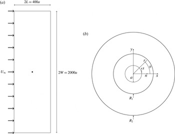
(a) Schematic of the computational domain used for the planar flow calculation; for axisymmetric flow, the domain is cut in half through the cylinder. The cylinder (of radius
 $r=a$
) is placed in a domain of width
 $2W$
and length
 $2L$
, where
 $W=1000a$
and
 $L=200a$
. In (b), the coordinate system used in this work is shown. Additionally the two circular regions of inner and outer radius (denoted by
 $R_{1}$
and
 $R_{2}$
), radius
 $1.2a$
and
 $5a$
, concentric to the cylinder are shown (figure not to scale).

For steady flows, the drag force can be expressed more generally in terms of the volume flux in the wake and source flow. Hunt & Eames (Reference Hunt and Eames2002) showed that in general, the drag force on a body (with no net momentum flux through the body surface) is
 $$\begin{eqnarray}\displaystyle F_{D}=-{\it\rho}Q_{s}U_{\infty }+2{\it\rho}Q_{w}U_{\infty }, & & \displaystyle\end{eqnarray}$$
where
 ${\it\rho}$
is density,
 $Q_{s}$
is the source flow generated by the body and
 $Q_{w}$
is the volume flux in the narrow downstream wake (the first term is usually described as the Lamb force – Lamb Reference Lamb1932). When
 $U_{b}=0$
, the source flow is equal to the volume flux in the wake (i.e.
 $Q_{w}=Q_{s}$
) and (2.13) reduces to the classic result attributed to Betz (Reference Betz1925):
 $$\begin{eqnarray}\displaystyle F_{D}={\it\rho}Q_{w}U_{\infty }. & & \displaystyle\end{eqnarray}$$
For a strong uniform sucking flow (
 $-{\it\Lambda}\gg 1$
), the boundary layer thickness for both cylinder and sphere scale as
 ${\it\nu}/|U_{b}|$
and the boundary layer is thin. As the flow is irrotational outside the thin attached boundary layer and downstream of the body, the wake volume flux
 $Q_{w}$
is negligible and the drag force tends to
 $$\begin{eqnarray}\displaystyle F_{D}=-{\it\rho}A_{b}U_{b}U_{\infty }({>}0), & & \displaystyle\end{eqnarray}$$
where
 $A_{b}$
is the surface area of the rigid body. The integral approach provides details of the drag force but does not give any insight into the flow field. Expression (2.15) was derived by Pankhurst & Thwaites (Reference Pankhurst and Thwaites1953, appendix I) for flows with strong suction and no thrust.
Much less general information can be gleaned for the case of a strong blow flow (
 ${\it\Lambda}\gg 1$
). From the general discussion of forces, the source flux
 $Q_{s}$
is a combination of the wake and blowing flux,
 $Q_{s}=Q_{w}+Q_{b}$
, which combined with (2.13) gives
 $$\begin{eqnarray}\displaystyle F_{D}={\it\rho}U_{\infty }(Q_{w}-A_{b}U_{b}), & & \displaystyle\end{eqnarray}$$
(also obtained by Cliffe & Lever (Reference Cliffe and Lever1985, equation (17)). As we shall see, a blowing flow causes the wake width to widen and the wake volume flux to increase, i.e.
 $Q_{w}\sim A_{b}U_{b}$
, so that the drag force is not as strongly affected by
 ${\it\Lambda}$
as compared to the dramatic effect of a sucking flow.
The kinematic effect of the rigid surface generates a source flow in the far field and a dipole contribution for a cylinder or sphere. The irrotational solution,
 $\boldsymbol{u}=\boldsymbol{{\rm\nabla}}{\it\phi}$
, is well known for a uniform flow past a flat plate (length
 $2a$
)
 $$\begin{eqnarray}\displaystyle {\it\phi}(r,{\it\theta})=U_{\infty }r\cos {\it\theta}+U_{b}r\sin {\it\theta}, & & \displaystyle\end{eqnarray}$$
for a cylinder
 $$\begin{eqnarray}\displaystyle {\it\phi}(r,{\it\theta})=U_{\infty }r\cos {\it\theta}\left(1+\frac{a^{2}}{r^{2}}\right)+U_{b}a\log r, & & \displaystyle\end{eqnarray}$$
and a sphere,
 $$\begin{eqnarray}\displaystyle {\it\phi}(r,{\it\theta})=U_{\infty }r\cos {\it\theta}\left(1+\frac{a^{3}}{2r^{3}}\right)-\frac{U_{b}a^{2}}{r}. & & \displaystyle\end{eqnarray}$$
The slip velocity at the surface of the rigid body in a potential flow is
 $\partial {\it\phi}/\partial s|_{r=a}=-U_{\infty }$
,
 $-2U_{\infty }\sin {\it\theta}$
or
 $-(3/2)U_{\infty }\sin {\it\theta}$
, (where
 $s=a{\it\theta}$
for a cylinder and sphere). To examine the influence of this component, we decompose the velocity into a primary irrotational component and a rotational component to enforce the no-slip condition on the rigid surfaces, i.e.
 $$\begin{eqnarray}\displaystyle \boldsymbol{u}=\boldsymbol{{\rm\nabla}}{\it\phi}+\boldsymbol{u}_{R}(\boldsymbol{x},t). & & \displaystyle\end{eqnarray}$$
The purpose of the discussion in this section is to examine the form and role of the rotational component of the flow, using a boundary layer analysis for short time, and a viscous description for blowing for long time. Much of the discussion will centre around the short blowing viscous (
 $T_{{\it\nu}}$
) and inertial (
 $T_{b}$
) time scales set by the blow velocity and the advective time scale (
 $T_{a}$
) defined as
 $$\begin{eqnarray}\displaystyle T_{{\it\nu}}=\frac{{\it\nu}}{U_{b}^{2}},\quad T_{b}=\frac{a}{|U_{b}|},\quad T_{a}=\frac{a}{U_{\infty }}. & & \displaystyle\end{eqnarray}$$
2.2 Viscously dominated flows (
$Re\rightarrow 0$
and
$Re_{b}\neq 0$
)


Klettner & Eames (Reference Klettner and Eames2015) analysed the low Reynolds number flow past a cylinder with uniform blowing or sucking. By assuming a symmetrical vorticity field (about
 ${\it\theta}={\rm\pi}/2$
), a leading-order solution to the Oseen form of the vorticity equation was constructed:
 $$\begin{eqnarray}\displaystyle \tilde{{\it\omega}}=\text{e}^{(Re/4)\tilde{r}\cos {\it\theta}}C_{1}\tilde{r}^{Re{\it\Lambda}/4}K_{(1+(Re{\it\Lambda}/4)^{2})^{1/2}}(Re\,\tilde{r}/4)\sin {\it\theta}, & & \displaystyle\end{eqnarray}$$
where
 $$\begin{eqnarray}\displaystyle C_{1}=\frac{2}{\displaystyle \int _{1}^{\infty }p_{1}(\tilde{r})\,\text{d}\tilde{r}}, & & \displaystyle\end{eqnarray}$$
and
 $$\begin{eqnarray}\displaystyle p_{1}(\tilde{r})=-\tilde{r}^{Re{\it\Lambda}/4}\frac{J_{1}(\text{i}Re\tilde{r}/4)}{\text{i}Re\tilde{r}/4}K_{(1+(Re{\it\Lambda}/4)^{2})^{1/2}}(Re\tilde{r}/4). & & \displaystyle\end{eqnarray}$$
The expression is valid for
 $Re\rightarrow 0$
and
 $-\infty <{\it\Lambda}<4/Re$
. The pressure and viscous drag coefficients are
 $$\begin{eqnarray}\displaystyle C_{P} & = & \displaystyle -C_{1}\frac{{\rm\pi}}{Re}\left((Re{\it\Lambda}/4+(1+(Re{\it\Lambda}/4)^{2})^{1/2})K_{(1+(Re{\it\Lambda}/4)^{2})^{1/2}}(Re/4)\phantom{\frac{Re}{4}}\right.\nonumber\\ \displaystyle & & \displaystyle +\left.\frac{Re}{4}K_{(1+(Re{\it\Lambda}/4)^{2})^{1/2}-1}(Re/4)\right),\end{eqnarray}$$
 $$\begin{eqnarray}\displaystyle C_{{\it\nu}} & = & \displaystyle -C_{1}\frac{{\rm\pi}}{Re}K_{(1+(Re{\it\Lambda}/4)^{2})^{1/2}}\left(Re/4\right),\end{eqnarray}$$
such that the ratio of the viscous drag to the total drag coefficient is
 $$\begin{eqnarray}\displaystyle \frac{C_{{\it\nu}}}{C_{D}}=\frac{1}{Re{\it\Lambda}/4+(1+(Re{\it\Lambda}/4)^{2})^{1/2}+1+{\displaystyle \frac{Re}{4}}{\displaystyle \frac{K_{(1+(Re{\it\Lambda}/4)^{2})^{1/2}-1}(Re/4)}{K_{(1+(Re{\it\Lambda}/4)^{2})^{1/2}}(Re/4)}}}. & & \displaystyle\end{eqnarray}$$
For strong suction,
 $$\begin{eqnarray}\displaystyle C_{D}\rightarrow -2{\rm\pi}{\it\Lambda}, & & \displaystyle\end{eqnarray}$$
which agrees with (2.15). The flux of vorticity, defined as
 $$\begin{eqnarray}\displaystyle F_{{\it\omega}}=\int _{0}^{{\rm\pi}}aU_{b}{\it\omega}_{s}\,\text{d}{\it\theta}, & & \displaystyle\end{eqnarray}$$
is
 $$\begin{eqnarray}\displaystyle \frac{F_{{\it\omega}}}{U_{\infty }^{2}}={\it\Lambda}C_{1}\frac{J_{1}(\text{i}Re/4)}{\text{i}Re/4}K_{(1+(Re{\it\Lambda}/4)^{2})^{1/2}}(Re/4). & & \displaystyle\end{eqnarray}$$
Dukowicz (Reference Dukowicz1982) analysed the Stokes flow (low
 $Re$
) past a blowing sphere, which, similar to the no-blowing case, admits a closed form expression for the flow field and force without the requirement of including an Oseen approximation. We repeat the main results of Dukowicz (Reference Dukowicz1982) (who includes advection and stretching of azimuthal vorticity caused by the blow flow) and show how they provide information for higher Reynolds number scenarios. Dukowicz’s analysis is strictly valid for
 $Re\ll 1$
and
 ${\it\Lambda}<0$
, such that the boundary layer is thin compared to the sphere radius. When
 ${\it\Lambda}>0$
, we require
 ${\it\Lambda}Re<1$
or
 ${\it\Lambda}<1/Re$
, which is similar to the cylinder case. Dukowicz (Reference Dukowicz1982) derived an expression for the drag on a rigid sphere for
 $Re\ll 1$
and finite values of
 ${\it\Lambda}Re$
and showed that the vorticity field is given by
 $$\begin{eqnarray}\displaystyle \tilde{{\it\omega}}=-6\tilde{r}\sin {\it\theta}\frac{1-\left(1+{\displaystyle \frac{1}{2}}Re{\it\Lambda}{\displaystyle \frac{1}{\tilde{r}}}+{\displaystyle \frac{1}{8}}Re^{2}{\it\Lambda}^{2}{\displaystyle \frac{1}{\tilde{r}^{2}}}\right)\exp \left(-{\displaystyle \frac{1}{2}}Re{\it\Lambda}{\displaystyle \frac{1}{\tilde{r}}}\right)}{\left(1+{\displaystyle \frac{1}{2}}Re{\it\Lambda}\right)\exp \left(-{\displaystyle \frac{1}{2}}Re{\it\Lambda}\right)-1+{\displaystyle \frac{1}{8}}Re^{2}{\it\Lambda}^{2}}. & & \displaystyle\end{eqnarray}$$
(The Reynolds number defined by Dukowicz (Reference Dukowicz1982) is based on the sphere radius, and not the diameter. This is why there is the additional factor of
 $1/2$
in the expressions stated in this paper.) For strongly sucking flow (
 $-{\it\Lambda}\gg 1$
), the vorticity decays exponentially away from the surface and
 $$\begin{eqnarray}\displaystyle \tilde{{\it\omega}}=-\frac{3}{2}\frac{Re|{\it\Lambda}|}{\tilde{r}^{2}}\sin {\it\theta}\exp \left(-{\displaystyle \frac{1}{2}}Re{\it\Lambda}\left(\frac{1}{\tilde{r}}-1\right)\right), & & \displaystyle\end{eqnarray}$$
which agrees with our later boundary layer analysis; while for blowing flows (
 ${\it\Lambda}\gg 1$
),
 $$\begin{eqnarray}\displaystyle \tilde{{\it\omega}}=\sin {\it\theta}\frac{{\displaystyle \frac{Re^{3}{\it\Lambda}^{3}}{8\tilde{r}^{2}}}\exp \left(-{\displaystyle \frac{1}{2}}Re{\it\Lambda}{\displaystyle \frac{1}{\tilde{r}}}\right)}{\left(1+{\displaystyle \frac{1}{2}}Re{\it\Lambda}\right)\exp \left(-{\displaystyle \frac{1}{2}}Re{\it\Lambda}\right)-1+{\displaystyle \frac{1}{8}}Re^{2}{\it\Lambda}^{2}}. & & \displaystyle\end{eqnarray}$$
The drag coefficient is
 $$\begin{eqnarray}\displaystyle C_{D}=8{\it\Lambda}\frac{1-\left(1+{\textstyle \frac{1}{2}}Re{\it\Lambda}\right)\exp \left(-{\textstyle \frac{1}{2}}Re{\it\Lambda}\right)}{\left(1+{\textstyle \frac{1}{2}}Re{\it\Lambda}\right)\exp \left(-{\textstyle \frac{1}{2}}Re{\it\Lambda}\right)-1+{\textstyle \frac{1}{8}}Re^{2}{\it\Lambda}^{2}}. & & \displaystyle\end{eqnarray}$$
For strongly sucking flows,
 $$\begin{eqnarray}\displaystyle C_{D}\rightarrow -8{\it\Lambda}, & & \displaystyle\end{eqnarray}$$
which agrees with (2.15). The fraction of the drag force that comes from the viscous stresses is
 $$\begin{eqnarray}\displaystyle \frac{C_{{\it\nu}}}{C_{D}}=\frac{4}{Re{\it\Lambda}}\frac{1-\left(1+{\textstyle \frac{1}{2}}Re{\it\Lambda}+{\textstyle \frac{1}{8}}Re^{2}{\it\Lambda}^{2}\right)\exp \left(-{\textstyle \frac{1}{2}}Re{\it\Lambda}\right)}{1-\left(1+{\textstyle \frac{1}{2}}Re{\it\Lambda}\right)\exp \left(-{\textstyle \frac{1}{2}}Re{\it\Lambda}\right)}, & & \displaystyle\end{eqnarray}$$
which at
 ${\it\Lambda}=0$
corresponds to a ratio of
 $2/3$
(for
 $Re\ll 1$
); the ratio
 $C_{{\it\nu}}/C_{D}$
only depends on
 $Re{\it\Lambda}$
. For strongly sucking flows,
 $C_{{\it\nu}}/C_{D}=1$
, while for strongly blowing flows,
 $C_{{\it\nu}}/C_{D}\sim 8/Re{\it\Lambda}$
. The flux of azimuthal vorticity from the sphere surface is
 $$\begin{eqnarray}\displaystyle F_{{\it\omega}}=\int _{0}^{{\rm\pi}}2{\rm\pi}a^{2}U_{b}{\it\omega}_{s}\sin {\it\theta}\,\text{d}{\it\theta}. & & \displaystyle\end{eqnarray}$$
Equation (2.37) can be written in dimensionless form
 $$\begin{eqnarray}\displaystyle \frac{F_{{\it\omega}}}{2aU_{\infty }^{2}}=\frac{3}{8}{\it\Lambda}{\rm\pi}^{2}\frac{1-\left(1+{\textstyle \frac{1}{2}}Re{\it\Lambda}+{\textstyle \frac{1}{8}}Re^{2}{\it\Lambda}^{2}\right)\exp \left(-{\textstyle \frac{1}{2}}Re{\it\Lambda}\right)}{\left(1+{\textstyle \frac{1}{2}}Re{\it\Lambda}\right)\exp \left(-{\textstyle \frac{1}{2}}Re{\it\Lambda}\right)-1+{\textstyle \frac{1}{8}}Re{\it\Lambda}^{2}}. & & \displaystyle\end{eqnarray}$$
In the limit of large sucking flows, the vorticity flux tends to
 $$\begin{eqnarray}\displaystyle \frac{F_{{\it\omega}}}{2aU_{\infty }^{2}}=\frac{3}{8}{\rm\pi}^{2}Re{\it\Lambda}^{2}. & & \displaystyle\end{eqnarray}$$
2.3 Unsteady boundary layer analysis (
$Re\gg 1$
and
$Re_{b}\gg 1$
)


At
 $t=0^{-}$
, the flow is irrotational and described by (2.17)–(2.19). When the flow is set into motion at
 $t=0$
, it must instantaneously adjust to the no-slip boundary condition applied at the rigid walls. For strongly sucking flows, the thickness of the boundary layer thickness scales as
 ${\it\delta}\sim {\it\nu}/|U_{b}|$
and as we shall see the flow is ultimately steady over a characteristic time scale
 $T_{{\it\nu}}$
given by (2.21). The boundary layer grows with time as it diffuses which is then balanced by convection resulting from the through-surface flow. When
 ${\it\Lambda}\gg 1$
, the boundary layer is blown away from the surface and initially
 ${\it\delta}\sim U_{b}t$
(
 ${\it\delta}\ll a$
).
To understand the development of the viscous and pressure forces with time, we first examine how the boundary layer develops in time. When the boundary layer thickness is much thinner than
 $a$
, the momentum equation tangential to the rigid surface for a flat plate (
 $\mathscr{D}=0$
), cylinder (
 $\mathscr{D}=1$
) and sphere (
 $\mathscr{D}=2$
) can be written, to leading order as
 $$\begin{eqnarray}\displaystyle \frac{\partial u_{s}}{\partial t}+U_{b}\left(\frac{a}{r}\right)^{\mathscr{D}}\frac{\partial u_{s}}{\partial r}=\frac{{\it\nu}}{r^{\mathscr{D}}}\frac{\partial }{\partial r}\left(r^{\mathscr{D}}\frac{\partial u_{s}}{\partial r}\right). & & \displaystyle\end{eqnarray}$$
Previous work on an impulsively started cylinder (e.g. Bar-Lev & Yang Reference Bar-Lev and Yang1975) and sphere (e.g. Basset Reference Basset1888) focussed around using the Rayleigh solution for a flat plate and projecting this onto a cylinder or sphere. The Rayleigh solution, which involves neglecting
 ${\it\nu}\mathscr{D}r^{-1}(\partial u_{s}/\partial r)$
, can be used to explain the unsteady viscous component of the drag force but cannot account for the pressure drag component, which depends on the normal gradient of the surface vorticity and would otherwise require a second-order solution (see for example Bar-Lev & Yang Reference Bar-Lev and Yang1975). We can explain the dependence of
 $C_{P}$
and
 $C_{{\it\nu}}$
on time and
 ${\it\Lambda}$
by writing
 $\tilde{t}=t/T_{a}$
,
 ${\tilde{n}}=(r-a)/a$
and
 $F_{1}=u_{s}/U_{\infty }$
. Equation (2.40) can then be rewritten as
 $$\begin{eqnarray}\displaystyle \frac{\partial F_{1}}{\partial \tilde{t}}=\frac{2}{Re}\frac{\partial ^{2}F_{1}}{\partial {\tilde{n}}^{2}}+\left(\frac{2\mathscr{D}}{Re}-{\it\Lambda}\right)\frac{\partial F_{1}}{\partial {\tilde{n}}}. & & \displaystyle\end{eqnarray}$$
The dimensionless tangential velocity is required to match across the no-slip condition the inner region of the outer flow. The solution corresponding to
 $F_{1}({\tilde{n}},\tilde{t})\rightarrow {\it\lambda}\sin {\it\theta}$
as
 ${\tilde{n}}\rightarrow \infty$
,
 $F_{1}(0,\tilde{t})=0$
,
 $F_{1}({\tilde{n}},0)=1$
is
 $$\begin{eqnarray}\displaystyle F_{1} & = & \displaystyle \left[1-{\displaystyle \frac{1}{2}}\left(\text{erfc}\left(\frac{{\tilde{n}}-({\it\Lambda}-2\mathscr{D}/Re)\tilde{t}}{\sqrt{8\tilde{t}/Re}}\right)\right.\right.\nonumber\\ \displaystyle & & \displaystyle +\!\left.\left.\exp \left(\frac{({\it\Lambda}-2\mathscr{D}/Re){\tilde{n}}}{2/Re}\right)\text{erfc}\left(\frac{{\tilde{n}}+({\it\Lambda}-2\mathscr{D}/Re)\tilde{t}}{\sqrt{8\tilde{t}/Re}}\right)\right)\right]{\it\lambda}\sin {\it\theta},\end{eqnarray}$$
where
 ${\it\lambda}=1,2$
and
 $3/2$
for a flat plate, cylinder and sphere, respectively and
 $\text{erfc}(z)=2/\sqrt{{\rm\pi}}\int _{z}^{\infty }\exp (-t^{2})\,\text{d}t$
(Abramowitz & Stegun Reference Abramowitz and Stegun1972). The
 $\sin {\it\theta}$
dependence is dropped for a flat plate. The vorticity at the rigid boundary is related to
 $F_{1}$
by
 $$\begin{eqnarray}\displaystyle \tilde{{\it\omega}}_{s} & = & \displaystyle -2\frac{\partial F_{1}}{\partial {\tilde{n}}}\bigg|_{{\tilde{n}}=0}=-2\left[\frac{(2\mathscr{D}-{\it\Lambda}Re)}{4}\left(1+\text{erf}\left(\frac{(2\mathscr{D}-{\it\Lambda}Re)\tilde{t}^{1/2}}{(8Re)^{1/2}}\right)\right)\right.\nonumber\\ \displaystyle & & \displaystyle \left.+\,\frac{1}{\sqrt{2{\rm\pi}\tilde{t}/Re}}\exp \left(-\frac{(2\mathscr{D}-{\it\Lambda}Re)^{2}\tilde{t}}{8Re}\right)\right]{\it\lambda}\sin {\it\theta}.\end{eqnarray}$$
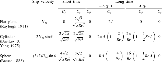
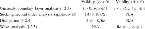
The force coefficients can then be calculated from (2.7)–(2.9). These results are summarised in table 1 with the range of validity in table 2 and the full expressions are given in appendix A.
Summary of the short and long time results of the unsteady boundary layer analysis where the slip velocity is the difference between the primary irrotational flow and zero tangential velocity imposed on the rigid surface. The full expressions are given in appendix A. The authors cited in brackets studied the relevant case for
 ${\it\Lambda}=0$
.

Summary of the validity of the present analysis.

2.4 Sucking flow (
${\it\Lambda}<0$
)

We explore in more detail the transient and steady force for strong sucking flow,
 $-{\it\Lambda}\gg 1$
, on these rigid bodies. For sucking flows, the vorticity in the boundary layer is to leading order
 $$\begin{eqnarray}\displaystyle \lim _{\tilde{t}\rightarrow \infty }\tilde{{\it\omega}}=-{\it\lambda}Re|{\it\Lambda}|\exp \left({\textstyle \frac{1}{2}}(2\mathscr{D}-Re|{\it\Lambda}|){\tilde{n}}\right)\sin {\it\theta}. & & \displaystyle\end{eqnarray}$$
The leading-order expressions for vorticity for the flow past a sucking cylinder and sphere are described by (B 14) and (C 11) respectively; these in turn reduce to (2.44) when
 $-{\it\Lambda}\gg 1$
.
The flux of vorticity through the surface from
 ${\it\theta}=0$
to
 ${\rm\pi}$
(or over a unit length of the surface), can be calculated from (2.44) giving
 $$\begin{eqnarray}\displaystyle \frac{F_{{\it\omega}}}{U_{\infty }^{2}}=Re{\it\Lambda}^{2},\quad \frac{F_{{\it\omega}}}{U_{\infty }^{2}}=2Re{\it\Lambda}^{2},\quad \frac{F_{{\it\omega}}}{2aU_{\infty }^{2}}=\frac{3}{8}{\rm\pi}^{2}Re{\it\Lambda}^{2}, & & \displaystyle\end{eqnarray}$$
for a flat plate, cylinder and sphere, respectively. The pressure gradient normal to the boundary layer is small and the surface pressure corresponds to the irrotational solution and does not contribute to the total drag force on the body. The pressure coefficient is
 $$\begin{eqnarray}\displaystyle C_{p}=1-4\sin ^{2}{\it\theta}-{\it\Lambda}^{2},\quad 1-{\textstyle \frac{9}{4}}\sin ^{2}{\it\theta}-{\it\Lambda}^{2}, & & \displaystyle\end{eqnarray}$$
for a cylinder/sphere, respectively. The first-order analysis (2.43), while quite an accurate description of the vorticity field, it is not able to recover the
 $\sin ^{2}{\it\theta}$
dependence seen in (2.46). A second-order analysis results in a pressure coefficient distribution of
 $$\begin{eqnarray}\displaystyle C_{p}({\it\theta})-C_{p}(0)=\frac{8}{Re}\left(1-\frac{2}{Re|{\it\Lambda}|}\right)(1-\cos {\it\theta})+\left(-1+\frac{6}{5Re|{\it\Lambda}|}\right)4\sin ^{2}{\it\theta}, & & \displaystyle\end{eqnarray}$$
where the first and second term on the right-hand side are the viscous and inviscid contributions, respectively. This analysis is presented in appendix B.
In the limit of
 $-{\it\Lambda}\gg 1$
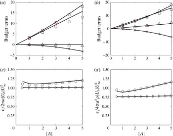
, the flow outside the boundary layer is irrotational and large gradients in the flow are confined to the boundary layer. This is a special case when the total dissipation in the entire body of fluid is finite and the energy equation can be applied to estimate the drag force. This dissipation technique is well known in the context of Levich’s (Reference Levich1949) estimate of the drag on a clean bubble (see Moore Reference Moore1963, Stone Reference Stone1992). From Landau & Lifshitz (Reference Landau and Lifshitz1966, p. 50), the unsteady form of the energy equation (in the frame of reference with the fluid at infinity at rest) is
 $$\begin{eqnarray}\displaystyle \int _{V-V_{B}}\frac{\partial }{\partial t}{\displaystyle \frac{1}{2}}{\it\rho}u^{2}\,\text{d}V=\int _{S_{B}+S_{\infty }}\left(-\boldsymbol{u}\left(p+{\displaystyle \frac{1}{2}}{\it\rho}u^{2}\right)+\boldsymbol{u}\boldsymbol{\cdot }{\bf\tau}\right)\boldsymbol{\cdot }\hat{\boldsymbol{n}}\,\text{d}S-{\it\epsilon}, & & \displaystyle\end{eqnarray}$$
where
 $S_{\infty }$
is a control surface far from the body. The viscous dissipation term
 ${\it\epsilon}$
(Batchelor Reference Batchelor1967, p. 174) is
 $$\begin{eqnarray}\displaystyle {\it\epsilon}=\frac{1}{2{\it\mu}}\int _{V-V_{B}}{\bf\tau}\boldsymbol{ : }{\bf\tau}\,\text{d}V\left(\equiv \int _{V-V_{B}}{\bf\tau}\boldsymbol{ : }\boldsymbol{{\rm\nabla}}\boldsymbol{u}\,\text{d}V\right), & & \displaystyle\end{eqnarray}$$
and is evaluated over the whole flow domain (
 $V$
) excluding the body (
 $V_{B}$
). To estimate the drag force, we must evaluate (2.48) in the frame of reference with the ambient flow at rest and the body moving.
In the far field the flow is irrotational, so that
 $p+{\it\rho}u^{2}/2=p_{\infty }-{\it\rho}\partial {\it\phi}/\partial t$
and the viscous stresses are weak. Therefore the contribution from the integral over
 $S_{\infty }$
reduces to
 $$\begin{eqnarray}\displaystyle \int _{S_{\infty }}p_{\infty }\boldsymbol{u}\boldsymbol{\cdot }\hat{\boldsymbol{n}}\,\text{d}S=\int _{S_{B}}U_{b}p\,\text{d}S, & & \displaystyle\end{eqnarray}$$
since the flux from the surface of the body is independent of the shape of
 $S_{\infty }$
. As the body moves with a constant velocity and the flow is steady in the moving frame, the left-hand side of (2.48) is
 $$\begin{eqnarray}\displaystyle \int _{V-V_{B}}\frac{\partial }{\partial t}{\displaystyle \frac{1}{2}}{\it\rho}u^{2}\,\text{d}V=\int _{V-V_{B}}(\boldsymbol{v}\boldsymbol{\cdot }\boldsymbol{{\rm\nabla}}){\displaystyle \frac{1}{2}}{\it\rho}u^{2}\,\text{d}V=\int _{S_{B}}\boldsymbol{v}\boldsymbol{\cdot }\hat{\boldsymbol{n}}{\displaystyle \frac{1}{2}}{\it\rho}u^{2}\,\text{d}S. & & \displaystyle\end{eqnarray}$$
Under these conditions, the right-hand side of (2.48) can be recast in terms of
 $$\begin{eqnarray}\displaystyle \boldsymbol{v}\boldsymbol{\cdot }\boldsymbol{F}=\int _{S_{B}}\boldsymbol{v}\boldsymbol{\cdot }(p\boldsymbol{I}-{\bf\tau})\boldsymbol{\cdot }\hat{\boldsymbol{n}}\,\text{d}S. & & \displaystyle\end{eqnarray}$$
Expressing the viscous stresses as
 ${\bf\tau}={\it\tau}_{n}\hat{\boldsymbol{n}}+{\it\tau}_{s}\hat{\boldsymbol{s}}$
and using the boundary conditions (2.1), (2.2), we can rewrite (2.48) in a general form:
 $$\begin{eqnarray}\displaystyle F_{D}U_{\infty }\equiv {\it\epsilon}+\int _{S_{B}}U_{b}\left(p+{\displaystyle \frac{1}{2}}{\it\rho}u^{2}-p_{\infty }-{\it\tau}_{n}\right)\,\text{d}S-\int _{S_{B}}(\boldsymbol{u}-\boldsymbol{v})\boldsymbol{\cdot }\boldsymbol{v}{\it\tau}_{s}\,\text{d}S. & & \displaystyle\end{eqnarray}$$
For a clean gas bubble the tangential shear stress is zero (
 ${\it\tau}_{s}=0$
) and
 $U_{b}=0$
, which reduces to Levich’s result that
 $F_{D}={\it\epsilon}/U_{\infty }$
. In our case, there is no tangential slip velocity and the last term is zero. We can estimate the various terms on the right-hand side of (2.53) for the case of a cylinder and sphere, using the boundary layer analysis for the velocity field.
For a cylinder, the flow (in the frame in which the far field is at rest) is approximately
 $$\begin{eqnarray}\displaystyle u_{{\it\theta}}=\frac{U_{\infty }a^{2}}{r^{2}}\sin {\it\theta}\!\left(1-2\text{e}^{(r-a)U_{b}/{\it\nu}}\right)\!,\quad u_{r}=-\frac{U_{\infty }a^{2}}{r^{2}}\cos {\it\theta}+\frac{U_{b}a}{r}. & & \displaystyle\end{eqnarray}$$
The dissipation term in polar coordinates is (Batchelor Reference Batchelor1967, p. 602)
 $$\begin{eqnarray}\displaystyle {\it\epsilon}=\int _{V-V_{B}}\left[2{\it\mu}\left(\left(\frac{\partial u_{r}}{\partial r}\right)^{2}+\left(\frac{1}{r}\frac{\partial u_{{\it\theta}}}{\partial {\it\theta}}+\frac{u_{r}}{r}\right)^{2}\right)+{\it\mu}\left(r\frac{\partial }{\partial r}\left(\frac{u_{{\it\theta}}}{r}\right)+\frac{1}{r}\frac{\partial u_{r}}{\partial {\it\theta}}\right)^{2}\right]\,\text{d}V. & & \displaystyle \nonumber\\ \displaystyle & & \displaystyle\end{eqnarray}$$
The dissipation can be decomposed into contributions from the boundary layer region (
 ${\it\epsilon}_{bl}$
), the radial blowing component (
 ${\it\epsilon}_{B}$
), non-blowing irrotational component outside the boundary layer (
 ${\it\epsilon}_{IR}$
) and the nonlinear interactions. The exponential terms decay sufficiently rapidly that the various components are estimated as
 $$\begin{eqnarray}\displaystyle {\it\epsilon}_{bl}=-2{\rm\pi}a{\it\rho}U_{b}U_{\infty }^{2},\quad {\it\epsilon}_{B}=4{\rm\pi}{\it\mu}U_{b}^{2},\quad {\it\epsilon}_{IR}=8{\rm\pi}{\it\mu}U_{\infty }^{2}, & & \displaystyle\end{eqnarray}$$
which gives a total dissipation of
 $$\begin{eqnarray}\displaystyle {\it\epsilon}\cong -2{\rm\pi}a{\it\rho}U_{b}U_{\infty }^{2}\left(1-\frac{4{\it\Lambda}}{Re}-\frac{8}{Re{\it\Lambda}}\right). & & \displaystyle\end{eqnarray}$$
A scaling analysis allows for an estimation of the radial distance where 99 % of each contribution occurs. For a cylinder the boundary layer, dipole and blowing contributions to the dissipation extend to
 ${\sim}\!2{\it\delta}$
(from the cylinder surface),
 ${\sim}\!10^{1/2}a$
and
 ${\sim}\!10a$
(from the cylinder centre) respectively.
The integral of the normal viscous stress over the surface of the cylinder is
 $$\begin{eqnarray}\displaystyle \int _{S_{B}}{\it\tau}_{n}\,\text{d}S\cong 4{\rm\pi}{\it\mu}U_{b}. & & \displaystyle\end{eqnarray}$$
As we have already discussed, the irrotational flow outside the boundary layer determines the pressure field at the cylinder surface and since the velocity normal to the cylinder surface is continuous,
 $$\begin{eqnarray}\displaystyle p+{\textstyle \frac{1}{2}}{\it\rho}u^{2}-p_{\infty }={\textstyle \frac{1}{2}}{\it\rho}(U_{\infty }^{2}\sin ^{2}{\it\theta}-u_{{\it\theta}}^{2})=0, & & \displaystyle\end{eqnarray}$$
because the tangential velocity is reversed in sign across the boundary layer. Combined together, we find for a cylinder
 $$\begin{eqnarray}\displaystyle C_{D}\cong \left({\it\epsilon}-U_{b}\int _{S_{B}}{\it\tau}_{n}\,\text{d}S\right)\bigg/\left(\frac{1}{2}{\it\rho}U_{\infty }^{3}2a\right)\cong 2{\rm\pi}|{\it\Lambda}|\left(1-\frac{8}{Re{\it\Lambda}}\right). & & \displaystyle\end{eqnarray}$$
For flow past a sphere, the flow (in the frame in which the far field is at rest) is
 $$\begin{eqnarray}\displaystyle u_{{\it\theta}}=\frac{U_{\infty }a^{3}}{2r^{3}}\sin {\it\theta}\left(1-3\text{e}^{(r-a)U_{b}/{\it\nu}}\right),\quad u_{r}=-\frac{U_{\infty }a^{3}}{r^{3}}\cos {\it\theta}+\frac{U_{b}a^{2}}{r^{2}}. & & \displaystyle\end{eqnarray}$$
For axisymmetric flows the dissipation term is
 $$\begin{eqnarray}\displaystyle {\it\epsilon} & = & \displaystyle \int _{V-V_{B}}\left[2{\it\mu}\left(\left(\frac{\partial u_{r}}{\partial r}\right)^{2}+\left(\frac{1}{r}\frac{\partial u_{{\it\theta}}}{\partial {\it\theta}}+\frac{u_{r}}{r}\right)^{2}\right),\right.\nonumber\\ \displaystyle & & \displaystyle +\left.{\it\mu}\left(r\frac{\partial }{\partial r}\left(\frac{u_{{\it\theta}}}{r}\right)+\frac{1}{r}\frac{\partial u_{r}}{\partial {\it\theta}}\right)^{2}+2{\it\mu}\left(\frac{u_{r}}{r}+\frac{u_{{\it\theta}}}{r}\cot {\it\theta}\right)^{2}\right]\,\text{d}V.\end{eqnarray}$$
The various components are estimated as
 $$\begin{eqnarray}\displaystyle {\it\epsilon}_{bl}=-3{\rm\pi}a^{2}{\it\rho}U_{b}U_{\infty }^{2},\quad {\it\epsilon}_{B}=16{\rm\pi}{\it\mu}U_{b}^{2}a,\quad {\it\epsilon}_{IR}=12{\rm\pi}{\it\mu}U_{\infty }^{2}a. & & \displaystyle\end{eqnarray}$$
In combination, the dissipation term is to leading order
 $$\begin{eqnarray}\displaystyle {\it\epsilon}\cong -3{\rm\pi}a^{2}{\it\rho}U_{b}U_{\infty }^{2}\left(1-\frac{32}{3}\frac{{\it\Lambda}}{Re}-\frac{8}{Re{\it\Lambda}}\right). & & \displaystyle\end{eqnarray}$$
For a sphere, a scaling analysis allows for an estimation of where 99 % of each contribution occurs, similar as that for a cylinder. For a sphere the boundary layer, dipole and blowing contributions to the dissipation extend to
 ${\it\epsilon}_{bl}\sim 2{\it\delta}$
(from the sphere surface),
 ${\it\epsilon}_{IR}\sim 3a$
and
 ${\it\epsilon}_{B}\sim 5a$
(from the sphere centre) respectively.
Now, on the surface of the sphere the pressure distribution is
 $$\begin{eqnarray}\displaystyle p+{\textstyle \frac{1}{2}}{\it\rho}u^{2}-p_{\infty }={\textstyle \frac{1}{2}}{\it\rho}(U_{\infty }^{2}\sin ^{2}{\it\theta}-u_{{\it\theta}}^{2})={\textstyle \frac{3}{8}}{\it\rho}U_{\infty }^{2}\sin ^{2}{\it\theta}, & & \displaystyle\end{eqnarray}$$
so the pressure contribution to the first integral on the right-hand side of (2.53), over the surface, is
 ${\rm\pi}a^{2}{\it\rho}U_{\infty }^{2}U_{b}$
. The viscous stress term is
 $$\begin{eqnarray}\displaystyle \int _{S_{B}}{\it\tau}_{n}\,\text{d}S\cong 16{\rm\pi}U_{b}{\it\mu}a. & & \displaystyle\end{eqnarray}$$
In total, we have
 $$\begin{eqnarray}\displaystyle \hspace{-15.00002pt}C_{D}\cong \left({\it\epsilon}-{\rm\pi}a^{2}{\it\rho}U_{b}U_{\infty }^{2}-U_{b}\int _{S_{B}}{\it\tau}_{n}\,\text{d}S\right)\bigg/\left(\frac{1}{2}{\it\rho}U_{\infty }^{3}2a\right)\cong 8|{\it\Lambda}|\left(1-\frac{6}{Re{\it\Lambda}}\right), & & \displaystyle\end{eqnarray}$$
which agrees with (2.15) for large
 $Re$
.
2.5 Blowing flow (
${\it\Lambda}>0$
)

For a large blow velocity, we expect the vorticity to form detached shear layers that bear a similarity to the shear layers that occur in other types of flows, for instance, flows past groups of bodies (Nicolle & Eames Reference Nicolle and Eames2011) or porous sheets (Castro Reference Castro1971). Typically, at some distance downstream, the shear layers become unstable and generate a von Kármán vortex street. During the initial phase, the vortex sheets are well separated and the decay in the maximum vorticity is due to diffusion which is a relatively slow process. This can be seen in the flow field figures 16(e–g) and 18(e–g) for a cylinder and sphere, respectively. Depending on the Reynolds number of the flow, the transition to a faster rate of decay is unlikely to be observed since it requires the vorticity in adjacent vortex lumps to merge and annihilate (see Hunt & Eames Reference Hunt and Eames2002).
The downstream flow signature is intrinsically linked to the forces acting the body. Insight can be gained by analysing the viscous and pressure contributions to the force on the body. In the limit of large
 ${\it\Lambda}$
, viscous effects are weak near the surface of the cylinder and the pressure is dominated by the vortex force term (
 $=\!{\it\rho}U_{b}{\it\omega}_{s}$
). Although the flow will be unsteady far downstream, a steady analysis can identify some of the critical physics of the wake flow and its connection with the near field. Focussing on the two-dimensional case in the limit of
 ${\it\Lambda}\gg 1$
, the vortical component of the flow is largely advected in the near field by the irrotational flow. A velocity jump of magnitude
 $\int _{SL}{\it\omega}\,\text{d}\boldsymbol{s}$
is generated across the shear layer (SL), downstream of the cylinder. Here the integral is taken across the streamline. Since the flow in the wake is much less than
 $U_{\infty }$
, then in the region
 $y>0$
,
 $$\begin{eqnarray}\displaystyle U_{\infty }\cong \int _{SL}{\it\omega}\,\text{d}\boldsymbol{s}\cong -\frac{F_{{\it\omega}}}{U_{\infty }}, & & \displaystyle\end{eqnarray}$$
which means that for
 ${\it\Lambda}\gg 1$
the vorticity flux through the cylinder surface is
 $$\begin{eqnarray}\displaystyle \frac{F_{{\it\omega}}}{U_{\infty }^{2}}\cong -1. & & \displaystyle\end{eqnarray}$$
The first term in the Fourier expansion of the vorticity field (
 $\tilde{{\it\omega}}_{s}\cong c_{1}\sin {\it\theta}$
) is
 $$\begin{eqnarray}\displaystyle c_{1}=\frac{F_{{\it\omega}}}{{\it\Lambda}U_{\infty }^{2}}, & & \displaystyle\end{eqnarray}$$
and this allows the pressure distribution and the drag force to be estimated. From (2.11), the surface pressure distribution is approximately
 $$\begin{eqnarray}\displaystyle C_{p}({\it\theta})-C_{p}(0)\cong -\frac{F_{{\it\omega}}}{U_{\infty }^{2}}(1-\cos {\it\theta}), & & \displaystyle\end{eqnarray}$$
and the drag coefficient is
 $$\begin{eqnarray}\displaystyle C_{D}\cong -{\displaystyle \frac{1}{2}}{\it\Lambda}\int _{0}^{2{\rm\pi}}\tilde{{\it\omega}}_{s}\sin {\it\theta}\,\text{d}{\it\theta}\cong -\frac{{\rm\pi}F_{{\it\omega}}}{2U_{\infty }^{2}}. & & \displaystyle\end{eqnarray}$$
We now extend our discussion to a blowing sphere. Again, taking the first term in the Fourier expansion of
 $\tilde{{\it\omega}}_{s}$
(i.e.
 $\tilde{{\it\omega}}=c_{1}\sin {\it\theta}$
), then the flux relationship is,
 $$\begin{eqnarray}\displaystyle \frac{F_{{\it\omega}}}{2aU_{\infty }^{2}}\cong \frac{{\rm\pi}^{2}{\it\Lambda}}{4}c_{1}. & & \displaystyle\end{eqnarray}$$
The pressure distribution is
 $$\begin{eqnarray}\displaystyle C_{p}({\it\theta})-C_{p}(0)\cong -\frac{4}{{\rm\pi}^{2}}\frac{F_{{\it\omega}}}{2aU_{\infty }^{2}}(1-\cos {\it\theta}), & & \displaystyle\end{eqnarray}$$
and the drag coefficient is estimated to be
 $$\begin{eqnarray}\displaystyle C_{D}\cong -\frac{32}{3{\rm\pi}^{2}}\frac{F_{{\it\omega}}}{2aU_{\infty }^{2}}. & & \displaystyle\end{eqnarray}$$
The flux of azimuthal vorticity is not conserved in axisymmetric flows because vortex stretching is important. Instead we must look at
 ${\it\omega}_{{\it\phi}}/y_{SL}$
(where
 $y_{SL}$
is the distance from the centreline) which is proportional to the circulation of the vortical element (Hunt & Eames Reference Hunt and Eames2002). The flux of
 ${\it\omega}_{{\it\phi}}/y_{SL}$
is conserved providing there is no vorticity annihilation so that in the shear layer,
 $$\begin{eqnarray}\displaystyle \int _{SL}\frac{{\it\omega}_{{\it\phi}}}{y_{SL}}\boldsymbol{u}\boldsymbol{\cdot }\text{d}\boldsymbol{s}=\text{const.}, & & \displaystyle\end{eqnarray}$$
where the integral is taken across the shear layer. When
 $Re\gg 1$
, since the flux of circulation is conserved along the shear layer until vorticity annihilation occurs,
 $$\begin{eqnarray}\displaystyle \int _{SL}\frac{{\it\omega}_{{\it\phi}}}{y_{SL}}U_{\infty }\,\text{d}s=\int _{0}^{{\it\theta}}\frac{{\it\omega}_{{\it\phi}}}{y_{SL}}U_{b}a\,\text{d}{\it\theta}, & & \displaystyle\end{eqnarray}$$
or
 $$\begin{eqnarray}\displaystyle \frac{U_{\infty }}{Y_{W}}\int _{SL}{\it\omega}_{{\it\phi}}\,\text{d}s=U_{b}{\rm\pi}\frac{U_{\infty }}{2a}c_{1}, & & \displaystyle\end{eqnarray}$$
where
 $Y_{W}$
is the ultimate distance of the shear layer from the centreline. As with the cylinder case, the velocity jump across the shear layer corresponds to
 $U_{\infty }$
; the ultimate wake width is estimated from the potential flow solution to be
 $Y_{W}/2a\sim {\it\Lambda}^{1/2}$
. Combined together, we estimate
 $$\begin{eqnarray}\displaystyle c_{1}=-\frac{2a}{{\rm\pi}Y_{W}{\it\Lambda}}\cong -\frac{1}{{\rm\pi}{\it\Lambda}^{3/2}}. & & \displaystyle\end{eqnarray}$$
This provides a closure to enable the leading-order terms to be estimated, i.e.
 $$\begin{eqnarray}\displaystyle \frac{F_{{\it\omega}}}{2aU_{\infty }^{2}}\cong -\frac{{\rm\pi}}{4{\it\Lambda}^{1/2}},\quad {\rm\Delta}C_{p}\cong \frac{2}{{\it\Lambda}^{1/2}{\rm\pi}},\quad C_{D}\cong \frac{8}{3{\rm\pi}{\it\Lambda}^{1/2}}. & & \displaystyle\end{eqnarray}$$
While these estimates are indicative and order of magnitude, they show that the vorticity flux and drag coefficient decrease with
 ${\it\Lambda}$
in contrast to the case of a cylinder. This is because the stretching of the azimuthal vorticity by the blowing flow means that a smaller surface vorticity is required to generate the step change of
 $U_{\infty }$
across the wake shear layer.
3 Numerical formulation
3.1 Geometry, solver and validation
Figure 2 shows a schematic of the finite computational domain, which for the two-dimensional problem has width
 $2W$
and length
 $2L$
; for an axisymmetric flow the domain radius was
 $W$
. We chose
 $W/a=1000$
and
 $L/a=200$
. The challenge is that the force calculations are sensitive to the finite size of the computational domain. The sensitivity is related to the fact that the boundary conditions imposed on the computational domain are
 $U_{\infty }\hat{\boldsymbol{x}}$
on the inlet surface, kinematic and no-slip condition on the rigid cylinder, zero flux on the sidewalls and a constant pressure constraint on the outlet. In addition to making the domain large, the boundary layer is extremely thin for the case of strongly sucking flows and high
 $Re$
. Typically
 $10$
points are used to resolve the boundary layer whose thickness scales as
 $1/|Re_{b}|$
, which for
 $Re=100$
and
 ${\it\Lambda}=-3$
, gives elements which have sides of length
 $0.0006a$
. For a blowing flow, the boundary layer is much thicker and elements of the size of
 $0.006a$
were found to be sufficient for
 $Re=100$
and their size could be further increased at lower
 $Re$
. The computational domain in the vicinity of the cylinder and sphere were refined in two circular regions (
 $R_{1}$
and
 $R_{2}$
) of radius
 $1.2a$
and
 $5a$
. The domain was meshed using Gmsh (Geuzaine & Remacle Reference Geuzaine and Remacle2009). Between
 $300\,000$
and
 $1.5\times 10^{6}$
nodes were used in the computations. The other challenge was that, in contrast to the non-blowing case where the smaller elements tend to be in the slowly moving part of the domain, in this case, the faster moving region of the flow coincided with the smallest elements, meaning that the time stepping constraint was severe, tending to be
 $10^{-6}U_{\infty }/a$
for
 $Re=100$
and
 ${\it\Lambda}=3$
.
The continuity and momentum equations were solved using an in-house code called ‘ACEsim’ with the characteristic based split scheme (Zienkiewicz, Taylor & Nithiarasu Reference Zienkiewicz, Taylor and Nithiarasu2005) which has been shown to be effective at studying fundamental fluid mechanics problems (Nicolle & Eames Reference Nicolle and Eames2011; Klettner & Eames Reference Klettner and Eames2012). The defining equations are solved in three steps: involving first the calculation of an intermediate velocity field using the forcing by the viscous forces. The second step is the calculation of the pressure field, from the fact that the Laplacian of pressure is proportional to the divergence of the intermediate velocity. The pressure is applied to force the intermediate velocity field to be solenoidal, and the updated velocity field is calculated in the third step. An axisymmetric formulation was developed, tested and applied in this paper.
3.2 Effect of boundedness on drag force
Flow boundedness has a significant influence on the drag calculations. We first discuss the influence of a domain size on the two-dimensional results. The bounding side walls generate a symmetric flow perturbation to the flow in the vicinity of the cylinder, which has a negligible effect on the drag force; but as a consequence of the finite length of the domain, a streamwise flow perturbation is generated in the vicinity of the cylinder. This perturbation (
 ${\rm\Delta}U$
), can be estimated using the method of images to account for the kinematic effect of the channel walls and the inlet condition. This technique has been used by Eames & Duursma (Reference Eames and Duursma1997) for a different problem. The perturbation is given by
 $$\begin{eqnarray}\displaystyle {\rm\Delta}U=\mathop{\sum }_{k=0,\pm 1,\pm 2,\ldots }\frac{{\rm\pi}U_{b}aW}{W^{2}+L^{2}k^{2}}=\frac{a{\rm\pi}U_{b}}{W}\left(1+\frac{W{\rm\pi}}{L}\coth \frac{W{\rm\pi}}{L}\right). & & \displaystyle\end{eqnarray}$$
The cylinder ‘sees’ an effective streamwise flow
 $U_{\infty }+{\rm\Delta}U$
. So for
 ${\it\Lambda}<0$
, the drag on a cylinder is
 $$\begin{eqnarray}\displaystyle F_{D}=-2{\rm\pi}{\it\rho}U_{b}U_{\infty }a\left(1+{\rm\Delta}U/U_{\infty }\right)\!. & & \displaystyle\end{eqnarray}$$
The drag coefficient in a bounded flow
 $C_{D}$
is related to an unbounded flow
 $C_{D_{\infty }}$
, for a sucking flow, through,
 $$\begin{eqnarray}\displaystyle C_{D}=\left(1+\frac{a{\rm\pi}{\it\Lambda}}{W}\left(1+\frac{W{\rm\pi}}{L}\coth \frac{W{\rm\pi}}{L}\right)\right)C_{D_{\infty }}. & & \displaystyle\end{eqnarray}$$
When the domain is wide (e.g.
 $L/W\gg 1$
), the correction to the drag is
 $a{\rm\pi}^{2}{\it\Lambda}/L$
(approximately 30 % of this comes from the nearest image source term). For example, a sucking flow
 ${\it\Lambda}=-3$
, where
 $L/a=200$
, we expect that the numerical calculations give a drag coefficient 15 % lower than the unbounded estimate. This technique can also be used to correct the vorticity distribution on the surface of the cylinder. For a blowing flow, we anticipate that
 $F_{D_{\infty }}\sim {\it\rho}C_{D_{\infty }}U_{\infty }^{2}$
where
 $C_{D_{\infty }}$
has a weak dependence on
 $U_{b}$
. In this case,
 $C_{D}\sim (1+{\rm\Delta}U/U_{\infty })^{2}C_{D_{\infty }}$
and the effect of flow boundedness leads to the drag coefficient being over predicted by 30 % for
 ${\it\Lambda}=3$
. It is so strong that it changes the reported trend that
 $C_{D}$
decreases with
 ${\it\Lambda}$
for cylinders (see later).
For axisymmetric (or three-dimensional) flows through a pipe of radius
 $L$
, a similar argument of point sources can be applied. In this case, we anticipate
 ${\rm\Delta}U\sim a^{2}U_{b}^{2}/L^{2}$
and decays so quickly with
 $L$
that we expect that its influence on the drag coefficient to be negligible.
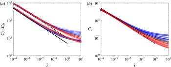
The characteristics of the drag force on a cylinder at
 $Re=1$
and
 ${\it\Lambda}=-3$
(▵),
 $-2~(+),-1$
(▹), 0 (○), 1 (▹), 2
 $(+)$
and 3 (▵). In (a), both the pressure coefficient (
 $C_{P}$
) and drag coefficient (
 $C_{D}$
) are plotted as functions of
 $t$
, normalised by the advective time scale. In (b), the viscous component of the drag coefficient (
 $C_{{\it\nu}}$
) is plotted as a function of
 $t$
, normalised by the advective time scale. The red and blue symbols correspond to
 ${\it\Lambda}>0$
and
 ${<}0$
, respectively. In (a) the solid and dashed lines are the pressure drag coefficient (A 2) and the total drag coefficient, respectively. The dashed line in (b) is the viscous drag coefficient (A 3).

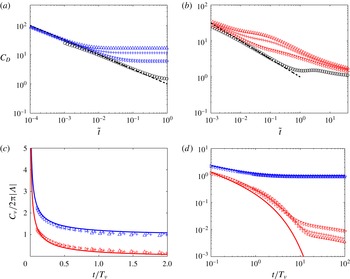
The characteristics of the drag coefficient and viscous force on a cylinder at
 $Re=100$
and
 ${\it\Lambda}=-3$
(▵),
 $-2~(+)$
,
 $-1$
(▹), 0 (○), 1 (▹), 2
 $(+)$
and 3
 $(\triangle )$
. In (a,b) the drag coefficient is shown as a function of
 $t$
, normalised by the advective time scale, for
 ${\it\Lambda}<0$
and
 ${>}0$
respectively. The viscous component of the drag force is plotted in (c,d); to highlight the different decay rates (for long and short time), the viscous force is plotted on a linear scale in (c) and logarithmic scale in (d). The dashed lines in (a,b) correspond to the total drag coefficient given by (A 2) and (A 3). The full lines in (c,d) are given by (A 3).

4 Unsteady drag forces
4.1 Cylinder
Figure 3(a,b) shows the variation of the pressure (
 $C_{P}$
), viscous (
 $C_{{\it\nu}}$
) and total drag (
 $C_{D}$
) coefficients with time for
 $Re=1$
. The blue symbols represent
 ${\it\Lambda}<0$
, black symbols
 ${\it\Lambda}=0$
and the red symbols
 ${\it\Lambda}>0$
. The total drag coefficient shows an initial weak dependence on
 ${\it\Lambda}$
. This is because the circulation across the thin boundary layer,
 ${\it\kappa}=\int _{0}^{\infty }{\it\omega}\,\text{d}n$
, depends only on the velocity outside the boundary layer, regardless of whether the flow is sucking or blowing, at least over the period that the boundary layer approximation is valid. The analysis in appendix C shows the variation of
 $C_{P}$
and
 $C_{{\it\nu}}$
for short time and confirms the
 $t^{-1/2}$
dependence observed numerically.
Figure 4 shows the results for
 $Re=100$
. The scalings for
 ${\it\Lambda}>0$
and
 ${<}0$
are sufficiently different that the drag coefficients must be plotted separately; for comparison the result for
 ${\it\Lambda}=0$
are included. The calculations for
 ${\it\Lambda}<0$
are run with a finer mesh to capture the thin boundary layer evolution and this results in a smaller time step than for
 ${\it\Lambda}>0$
. Note that to make the comparison easier, the results are normalised by the advective time scale
 $T_{a}$
. Figure 4(a,b) confirms that for short time, the drag coefficient decays as
 $t^{-1/2}$
and is weakly dependent on the blow velocity. For
 ${\it\Lambda}<0$
,
 $C_{D}$
has tended to a constant in a time that depends on
 $T_{{\it\nu}}$
. For
 ${\it\Lambda}>0$
, the drag force settles to a steady state over a time that depends on both
 $T_{a}$
and
 $T_{b}$
. The normalised viscous component of the force is plotted against time in figure 4(c,d) on linear and logarithmic scales. There is good agreement with (A 3) confirming that the drag coefficient scales as
 $2{\rm\pi}|{\it\Lambda}|$
and that this component decays over a time scale of
 $T_{{\it\nu}}$
. Figure 4(d) shows that the viscous component has an initial
 $t^{-1/2}$
dependence which is consistent with the boundary layer analysis. The later decay is exponential for the blowing case, up to when the viscous boundary layer becomes thick and streamwise advection becomes important. The pressure component to the total drag force is more difficult to interpret largely because the blowing time scale is comparable to the advective time scale.
4.2 Sphere
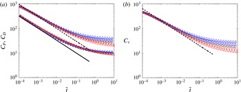
The results for the axisymmetric flow past a sphere with a through-surface flow, mirrors closely the observations for a cylinder. For
 $Re=1$
, figure 5(a,b) shows that the majority of the force has a viscous component with both the viscous and pressure components decaying as
 $t^{-1/2}$
. The pressure component in this case is one-third of the total drag force. This is consistent with the unsteady boundary layer analysis which is summarised in table 1 with the full expressions given in appendix A.
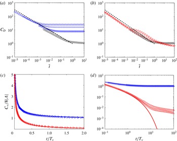
Figure 6 shows the variation of the total drag coefficient at
 $Re=100$
. Over a time scale of
 ${\sim}\!T_{{\it\nu}}$
the drag quickly decays to a steady state for
 ${\it\Lambda}<0$
and the initial decrease is
 $t^{-1/2}$
, in a similar manner to the cylinder. As with the case of the cylinder the initial development of the boundary layer structure largely explains the initial decrease of the viscous component of the force. The pressure component to the total drag force for
 ${\it\Lambda}<0$
is negligible and forms less than 2 % of the total force. For
 ${\it\Lambda}>0$
, the pressure component partially collapses for intermediate values of
 $t/T_{b}$
up to
 $5T_{b}$
, after which the decay for strong blowing decreasing as
 $t^{1/6}$
before asymptoting to a constant value.
The characteristics of the drag, pressure and viscous coefficient on a sphere at
 $Re=1$
and
 ${\it\Lambda}=-3$
(▵),
 $-2~(+)$
,
 $-1$
(▹), 0 (○), 1 (▹), 2
 $(+)$
and 3 (▵). In (a), both the pressure coefficient (
 $C_{P}$
) and drag coefficient (
 $C_{D}$
) are plotted as functions of
 $t$
, where
 $t$
is normalised by the advective time scale. In (b), the viscous component of the drag coefficient (
 $C_{{\it\nu}}$
) are plotted as a function of
 $t$
, normalised by the advective time scale. The red and blue symbols correspond to
 ${\it\Lambda}>0$
and
 ${<}0$
, respectively. In (a) the solid and dashed lines are the pressure drag coefficient (A 4) and the total drag coefficient respectively. The dashed line in (b) is the viscous drag coefficient (A 5).

The characteristics of the drag force on a sphere at
 $Re=100$
and
 ${\it\Lambda}=-3$
(▵),
 $-2~(+)$
,
 $-1$
(▹), 0 (○), 1 (▹), 2
 $(+)$
and 3 (▵). The drag coefficient is shown as a function of
 $t$
, normalised by the advective time scale, for
 ${\it\Lambda}<0$
(a) and
 ${>}0$
(b). In (a,b) the dashed lines correspond to the decay
 $t^{-1/2}$
. To highlight the different decay rates (for short and long time), the viscous component of the drag force is plotted on a linear scale in (c) and logarithmic scale in (d). The dashed lines in (a,b) correspond to the total drag coefficient given by (A 4) and (A 5). The full lines in (c,d) are given by (A 5).

The influence of
 ${\it\Lambda}$
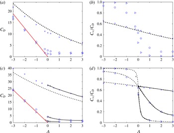
on the drag coefficient for a cylinder and sphere are shown in (a,c) respectively for
 $Re=1$
(
 $\times$
), 10 (○), 100 (▹). The fraction of the total drag coefficient which is due to viscous effects as a function of
 ${\it\Lambda}$
is shown in (b,d) indicating that the force is predominately viscous dominated for sucking flows (
 ${\it\Lambda}<0$
) and pressure dominated for blowing flows (
 ${\it\Lambda}>0$
). The red line in (a) and (c) is the asymptotic expression
 $2{\rm\pi}|{\it\Lambda}|$
. The dashed curves in (a) and (b) correspond to (2.26) and (2.27) (from Klettner & Eames Reference Klettner and Eames2015). The dashed curves in (c) and (d) correspond to (2.34) and (2.36) (from Dukowicz Reference Dukowicz1982). The black curves in (c) and (d) correspond to the numerical results of Cliffe & Lever (Reference Cliffe and Lever1985). The numerical results of Bagchi (Reference Bagchi2007) are shown in (c) and (d) (
 $+$
).

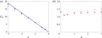
The steady drag coefficient for a cylinder at
 $Re=100$
is plotted as a function of
 ${\it\Lambda}$
as ▹. The drag coefficient is corrected for flow boundedness and plotted in (a,b) as a filled ▹ for
 ${\it\Lambda}<0$
and
 ${\it\Lambda}>0$
respectively and the corrected drag coefficient is
 $C_{D}=(1+{\rm\Delta}U/U_{\infty })C_{D_{\infty }}$
and
 $C_{D}=(1+{\rm\Delta}U/U_{\infty })^{2}C_{D_{\infty }}$
respectively.

5 Steady drag forces
5.1 Cylinder
The steady drag coefficients for
 $|{\it\Lambda}|\leqslant 3$
are shown in figure 7(a) for
 $Re=1,10$
and
 $100$
; the fraction of the total force due to viscous stresses is shown in figure 7(b).
The influence of the sucking flow has a dramatic effect on the drag coefficient, as shown in figure 7(a). For
 $Re=10$
and
 $100$
, the drag coefficient shows an approximately linear increase with
 $-{\it\Lambda}$
, in accordance with the boundary layer analysis summarised in table 1. For a blowing flow, the numerical results show that the drag coefficient has a weak dependence on
 ${\it\Lambda}$
, with a small tendency of
 $C_{D}$
to increase with
 ${\it\Lambda}$
. In comparison Mathelin et al. (Reference Mathelin, Bataille and Lallemand2002) found that the drag coefficient increased by nearly 30 % for
 ${\it\Lambda}=2$
(relative to
 ${\it\Lambda}=0$
) for a cylinder at
 $Re=3900$
. However, the domain width was only
 $10D$
and would have had a significant effect on the drag coefficient. The drag coefficient, in the present work, corrected for flow boundedness is shown for a cylinder and
 $Re=100$
in figure 8(a,b). The correction is as much as
 $15\,\%$
for
 ${\it\Lambda}=-3$
even though the flow domain is extremely large, tending to raise the drag coefficient for
 ${\it\Lambda}<0$
. In addition figure 8(b) shows that correcting for flow boundedness an increase of
 $C_{D}$
is not evident for
 ${\it\Lambda}>0$
.
In the sucking regime and
 $Re\geqslant 10$
, the drag force is largely dominated by the viscous component for
 ${\it\Lambda}<0$
and pressure component for
 ${\it\Lambda}>0$
, which is consistent with the mathematical models. For
 $Re=1$
, the variation of the viscous component with
 ${\it\Lambda}$
is 30 % over the range of
 ${\it\Lambda}$
considered, with
 $C_{{\it\nu}}/C_{D}\cong 1/2$
. For the strongly blowing case, (2.72) suggests
 $C_{D}\cong 1.55$
which is close to
 $C_{D}\cong 1.3$
(figure 8
b).
5.2 Sphere
The steady drag coefficient for
 $|{\it\Lambda}|\leqslant 3$
is shown in figure 7(c) for
 $Re=1,10$
and
 $100$
. The influence of flow boundedness is negligible for a sphere, which explains the excellent agreement between calculations and predictions for
 $Re=100$
. The results for
 $Re=1,10,100$
and
 ${\it\Lambda}>0$
agree with the curve from Cliffe & Lever (Reference Cliffe and Lever1985) and Bagchi (Reference Bagchi2007) confirming that for
 $Re<100$
,
 $C_{D}$
decreases as
 ${\it\Lambda}$
increases. The theoretical prediction by Dukowicz (Reference Dukowicz1982) is plotted for comparison, which gives a good agreement up to
 $Re=100$
.
The fraction of the drag force which arises from viscous stresses is shown in figure 7(d). For
 $Re=1$
, the viscous force is approximately two-thirds of the total force. At higher
 $Re$
, the drag force is largely dominated by viscous forces for
 ${\it\Lambda}<0$
and pressure forces for
 ${\it\Lambda}>0$
, consistent with the present mathematical model. The theoretical prediction (2.36) for
 $C_{{\it\nu}}/C_{D}$
by Dukowicz (Reference Dukowicz1982) agrees with the numerical results for
 $Re=1$
. For the strongly blowing case, (2.80) suggests
 $C_{D}\cong 0.9/{\it\Lambda}^{1/2}$
. For
 $Re=100$
and
 ${\it\Lambda}=3$
this gives a prediction of
 $C_{D}\cong 0.52$
which is close to the numerical simulation of
 $C_{D}\cong 0.5$
(figure 7
c).
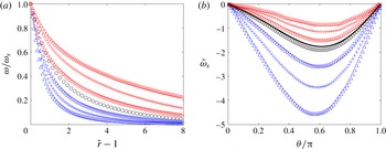
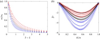
Vorticity distribution in the boundary layer of a cylinder at
 $Re=1$
, where
 ${\it\Lambda}=-3$
(▵),
 $-2~(+)$
,
 $-1$
(▹), 0 (○), 1 (▹), 2
 $(+)$
and 3 (▵). In (a), the vorticity through the boundary layer along the line of
 ${\it\theta}={\rm\pi}/2$
, normalised by its value at
 $\tilde{r}=1$
. In (b), the vorticity distribution over the surface of the cylinder. The black line in (b) is from Dennis & Shimshoni (Reference Dennis and Shimshoni1965) for
 ${\it\Lambda}=0$
.

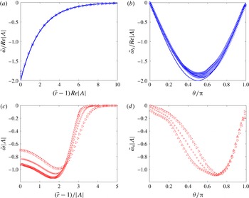
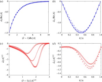
Vorticity distribution in the boundary layer of a cylinder at
 $Re=100$
, where
 ${\it\Lambda}=3$
(▵), 2
 $(+)$
, 1 (▹), 0 (○),
 $-1$
(▹),
 $-2~(+)$
and
 $-3$
(▵). In (a,c) the vorticity through the boundary layer, along the line
 ${\it\theta}={\rm\pi}/2$
, is plotted; while in (b,d) the vorticity on the surface of the cylinder is plotted. The blue curve in (a,b) corresponds to (2.44).

Vorticity distribution in the boundary layer of a sphere at
 $Re=1$
, where
 ${\it\Lambda}=-3$
(▵),
 $-2~(+)$
,
 $-1$
(▹), 0 (○), 1 (▹), 2
 $(+)$
and 3 (▵). In (a), the vorticity through the boundary layer along the line of
 ${\it\theta}={\rm\pi}/2$
, normalised by its value at
 $\tilde{r}=1$
. In (b), the vorticity distribution over the surface of the sphere. The full curves correspond to the results of Cliffe & Lever (Reference Cliffe and Lever1985) for
 ${\it\Lambda}=0,1,3$
. (Note,
 ${\it\Lambda}=2$
was not calculated by Cliffe & Lever (Reference Cliffe and Lever1985).)

Vorticity distribution in the boundary layer of a sphere at
 $Re=100$
, for
 ${\it\Lambda}=-1$
(▹),
 $-2~(+)$
,
 $-3$
(▵) and 3 (▵), 2
 $(+)$
, 1 (▹) respectively. In (a,c) the vorticity through the boundary layer, along the line
 ${\it\theta}={\rm\pi}/2$
, is plotted; while in (b,d) the vorticity on the surface of the sphere is plotted. The blue curve in (a,b) corresponds to (2.44).

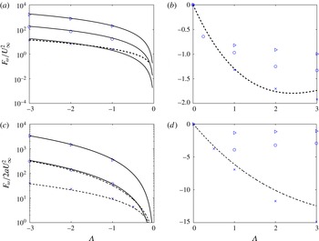
Vorticity flux through the surface of (a,b) cylinder and (c,d) sphere for
 $Re=1$
(
 $\times$
), 10 (○), 100 (▹). On the left-hand side, the flow is sucking, while on the right-hand side the flow is blowing. In (a,c) the strong sucking prediction given by (2.45) respectively, are plotted with full lines. In (a,b) and (c,d) the dashed lines correspond to low Reynolds number predictions given by (2.30) and (2.38) respectively.

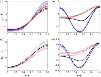
Pressure distribution on the surface of a cylinder (a,b) and sphere (c,d) for
 ${\it\Lambda}=1$
(▹), 2
 $(+)$
, 3 (▵) and
 $-3$
(▵),
 $-2$
 $(+)$
,
 $-1$
(▹) respectively. In (a,c),
 $Re=1$
, while for (b,d),
 $Re=100$
. The full blue curves in (b,d) correspond to the potential flow prediction (2.46). The full black lines in (a–d) correspond to the numerical calculations by Dennis & Shimshoni (Reference Dennis and Shimshoni1965), Berthelsen & Faltinsen (Reference Berthelsen and Faltinsen2008), Le Clair, Hamielec & Pruppacher (Reference Le Clair, Hamielec and Pruppacher1970) and Lee (Reference Lee2000) respectively.

6 Boundary layer structure
6.1 Vorticity field
6.1.1 Cylinder
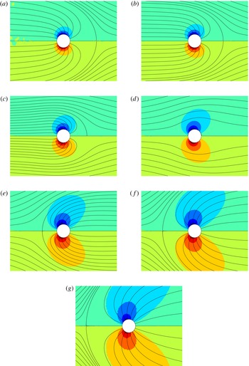
The boundary layer structure of the vorticity field is shown in figure 9 for
 $Re=1$
. A sucking flow increases the rate at which vorticity decays from the cylinder and also increases the magnitude of surface vorticity. A blowing flow decreases the magnitude of surface vorticity and decreases the rate at which the vorticity decays with distance from the surface. A comparison is shown between the numerical results and the theoretical predictions of Dennis & Shimshoni (Reference Dennis and Shimshoni1965) for
 ${\it\Lambda}=0$
. The small disagreement is accounted for by the effect of flow boundedness in the simulations.
Vorticity field and streamlines for a cylinder at
 $Re=1$
. The images correspond to
 ${\it\Lambda}=$
(a)
 $-3$
, (b)
 $-2$
, (c)
 $-1$
, (d)
 $0$
, (e)
 $1$
, (f)
 $2$
and (g)
 $3$
. The vorticity is normalised so its value extends over the range
 $-1$
(blue) to 1 (red).

For
 $Re=100$
and
 ${\it\Lambda}<0$
, we find that the surface vorticity decreases over a distance of
 $10a/(Re|{\it\Lambda}|)$
(figure 10
a,b). The boundary layer thickness can be calculated where
 $u_{s}({\it\delta})=0.99\partial {\it\phi}/\partial s|_{n=0}$
where
 $u_{s}$
is given by (2.42) for
 $\tilde{t}\rightarrow \infty$
and is
 ${\it\delta}/a\approx 9.2/(Re|{\it\Lambda}|)$
, which is consistent with figure 10(a). Similarly a momentum thickness can be calculated which is
 ${\it\theta}/a=1/(Re|{\it\Lambda}|)$
. The surface vorticity scales as
 $Re|{\it\Lambda}|$
and has a sine dependence on
 ${\it\theta}$
. The agreement with the theoretical predictions for
 ${\it\Lambda}<0$
is good; taking into account the influence of flow boundedness improves the agreement between the numerical calculations and the analytical results – notice the largest disagreement of 15 % occurs with the highest magnitude of
 ${\it\Lambda}$
.
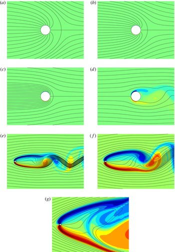
Vorticity field and streamlines for a blowing cylinder at
 $Re=100$
. The images correspond to
 ${\it\Lambda}=$
(a)
 $-3$
, (b)
 $-2$
, (c)
 $-1$
, (d)
 $0$
, (e)
 $1$
, (f)
 $2$
and (g) 3. The vorticity is normalised so its value extends over the range
 $-1$
(blue) to 1 (red).

For
 $Re=100$
and
 ${\it\Lambda}>0$
, the influence of advection becomes much more pronounced. figure 10(c,d) shows the vorticity distribution for
 $Re=100$
along the line
 ${\it\theta}={\rm\pi}/2$
and
 ${\it\Lambda}=1,2$
and
 $3$
. The scalings serve to demonstrate that the surface vorticity decreases approximately as
 ${\it\Lambda}^{-1}$
in the vicinity of the cylinder (figure 10
d) and has a lateral extend which increases with
 ${\it\Lambda}$
(figure 10
c).
6.1.2 Sphere
The boundary layer structure of the vorticity field is shown in figure 11 for
 $Re=1$
. A sucking flow increases the rate at which vorticity decays from the sphere and also increases the surface vorticity magnitude; blowing generates the opposite trend. A comparison is shown in figure 11(b) for
 ${\it\Lambda}=0,1$
and
 $3$
(taken from Cliffe & Lever (Reference Cliffe and Lever1985)); the agreement is good.
The trend for the boundary layer on a sphere at
 $Re=100$
follows that of the cylinder, for
 $Re=100$
which can be seen in figure 12(a,b). For a sucking flow, we see excellent agreement between the numerical calculations and (2.43). Since the influence of flow boundedness is greatly reduced for axisymmetric flows, the agreement for the distribution of vorticity on the surface is excellent, particularly at higher values of
 $|{\it\Lambda}|$
. Similar as to the cylinder a boundary layer and momentum thickness can be calculated which are
 $9.2/(Re|{\it\Lambda}|)$
and
 $1/(Re|{\it\Lambda}|)$
, respectively.
Figure 12(c,d) shows the vorticity field along
 ${\it\theta}={\rm\pi}/2$
and on the surface of the sphere for a blowing flow. The vorticity increases with distance from the sphere until it reaches a shear layer, represented as the local minimum, and then decreases rapidly in the dominant incident irrotational flow. The approximate collapse of the data in figure 12(d) serves to indicate that the vorticity scales as
 ${\it\Lambda}^{-3/2}$
in the vicinity of the sphere.
6.2 Vorticity flux
6.2.1 Cylinder
The convective flux of vorticity from the surface of the cylinder is shown in figure 13. For
 ${\it\Lambda}<-0.5$
, the convective flux of vorticity scales as
 $Re{\it\Lambda}^{2}$
as confirmed in figure 13(a). Including a correction due to the boundedness of the domain improves the agreement between the predictions and calculations. For blowing flows, we observe a weak dependence of the flux of vorticity on
 ${\it\Lambda}$
which is consistent with the scaling
 $\tilde{{\it\omega}}_{s}\sim 1/{\it\Lambda}$
and (2.69) and can be seen in figure 13(b). By considering only the first term in the Fourier expansion of the surface vorticity a leading-order estimate can be made for the drag coefficient
 $C_{D}\approx {\rm\pi}F_{{\it\omega}}/2U_{\infty }^{2}\sim 1.5$
, which is consistent with the numerical calculations corrected for a bounded domain (figure 8
b).
6.2.2 Sphere
Figure 13(c,d) shows the vorticity flux for a sphere with sucking and blowing flows respectively. The agreement with Dukowicz (Reference Dukowicz1982) is good for
 ${\it\Lambda}<1$
for
 $Re=1,10$
and good for
 ${\it\Lambda}>0$
and
 $Re=1$
. For
 ${\it\Lambda}>0$
, (2.80) suggests that
 $F_{{\it\omega}}$
decreases in magnitude as
 ${\it\Lambda}$
increases and the magnitude is consistent with (2.80). The drag force can be estimated using (2.80) which suggests that
 $C_{D}\cong 0.9/{\it\Lambda}^{1/2}$
. For
 $Re=100$
and
 ${\it\Lambda}=3$
this gives a prediction of
 $C_{D}\cong 0.52$
which is close to the numerical simulation of
 $C_{D}\cong 0.5$
(figure 7
c).
6.3 Surface pressure
6.3.1 Cylinder
The steady pressure distribution is shown in figure 14(a,b) for
 $Re=1$
and 100 respectively. For
 $Re=1$
, the pressure at the front is greater than at the rear – with a noticeable asymmetry due to inertia. For
 $Re=100$
, the upstream component of pressure corresponds to a value close to the irrotational prediction. For
 ${\it\Lambda}<0$
, the boundary layer is thin, the pressure is constant across the boundary layer and the surface pressure agrees with the irrotational prediction, as shown in figure 14(b). For
 ${\it\Lambda}=0$
(figure 14
b), the pressure distribution agrees closely to the potential flow prediction at the front and is approximately constant on the rear of the cylinder. The results are compared to previous numerical simulations; the disagreement with Dennis & Shimshoni (Reference Dennis and Shimshoni1965) at the rear of the cylinder is due to the effect of flow boundedness which is significant at
 $Re=1$
while good agreement is found at
 $Re=100$
with the numerical simulations of Berthelsen & Faltinsen (Reference Berthelsen and Faltinsen2008). The pressure distribution has a weak dependence on
 ${\it\Lambda}$
for
 ${\it\Lambda}>0$
(see figure 14
b), and this is consistent with the scalings in § 2.5. The pressure difference between the front and rear of the cylinder can be related to the convective flux. For
 $Re\gg 1$
, figure 14(b) shows
 ${\rm\Delta}C_{p}=C_{p}({\rm\pi})-C_{p}(0)\approx 1.8$
, which is consistent with (2.71) which estimates
 ${\rm\Delta}C_{p}\sim 2$
.
6.3.2 Sphere
The steady pressure distribution is shown in figures 14(c,d). For
 $Re=1$
, the pressure field shows a similar trend as for a cylinder, with the pressure being greater at the front than at the rear. For
 $Re=100$
and
 ${\it\Lambda}<0$
, the boundary layer is thin, the pressure is constant across the boundary layer and the surface pressure conforms to the irrotational prediction, as shown in figure 14(c). For
 ${\it\Lambda}=0$
(figure 14
d), the pressure distribution agrees closely to the potential flow prediction at the front of the sphere, with an approximately constant pressure distribution in the rear of the sphere. Good comparison with previous numerical simulations, for
 ${\it\Lambda}=0$
, is found in both cases. The pressure distribution has a weak dependence on
 ${\it\Lambda}>0$
(see figure 14
d). The pressure drop
 ${\rm\Delta}C_{p}$
from (2.71) is comparable to observations in figure 14(c) and
 ${\rm\Delta}C_{p}$
decreases with
 ${\it\Lambda}$
.
7 Flow field
7.1 Cylinder
Figures 15 and 16 show the vorticity distribution (with blue, green and red representing negative, zero and positive vorticity, respectively) and streamlines in the vicinity of a cylinder for
 $Re=1$
and
 $Re=100$
respectively. In all the figures depicting flow fields the flow is from left to right.
For
 $Re=1$
, a weak asymmetry in the flow is clearly observed for
 ${\it\Lambda}=0$
, indicating that inertia is still present. We also observe that the radial extent of the vorticity field increases with
 ${\it\Lambda}$
(for a blowing flow) and decreases for sucking flows (as confirmed in figure 15).
The influence of
 ${\it\Lambda}$
on the vorticity distribution is more pronounced at
 $Re=100$
. For
 ${\it\Lambda}<0$
, the boundary layer is extremely thin and is localised around the cylinder surface. Outside the boundary layer, the flow is irrotational. For
 ${\it\Lambda}>0$
, the vortex sheets that are formed by the blowing flow separate the positive and negative vorticity which is advected downstream. For
 $t<50T_{a}$
, a vortex bubble forms downstream of the cylinder which is ultimately unstable and is then shed downstream. The remnants of the vortex bubble (i.e. the large blue and red regions of vorticity between the shear layers) can be seen in figure 16(g) for
 ${\it\Lambda}=3$
. The vorticity in the shear layers decreases due to local cross-stream diffusion. Further downstream the vortex shear layers become unstable and form a von Kármán vortex sheet, as shown in figure 16(e,f) for
 ${\it\Lambda}=1,2$
respectively.
7.2 Sphere
Figures 17 and 18 shows the vorticity distribution downstream of a sphere for
 $Re=1$
and
 $Re=100$
respectively. The calculations are axisymmetric and reflected along the central axis.
Vorticity field and streamlines for a blowing sphere at
 $Re=1$
. The images correspond to
 ${\it\Lambda}=$
(a)
 $-3$
, (b)
 $-2$
, (c)
 $-1$
, (d)
 $0$
, (e)
 $1$
, (f)
 $2$
and (g)
 $3$
. The vorticity is normalised so its value extends over the range
 $-1$
(blue) to 1 (red).

Vorticity field and streamlines for a blowing sphere at
 $Re=100$
. The images correspond to
 ${\it\Lambda}=$
(a)
 $-3$
, (b)
 $-2$
, (c)
 $-1$
, (d)
 $0$
, (e)
 $1$
, (f)
 $2$
and (g)
 $3$
. The vorticity is normalised so its value extends over the range
 $-1$
(blue) to 1 (red).

The variation of the components of (2.60) and (2.67) for different blowing velocities at
 $Re=100$
for (a) a cylinder and (b) a sphere respectively;
 $F_{D}U_{\infty }$
(▫);
 ${\it\epsilon}$
(○);
 $U_{b}\int _{S_{B}}(p+(1/2){\it\rho}u^{2}-p_{\infty })\,\text{d}S$
(▵);
 $-U_{b}\int _{S_{B}}{\it\tau}_{n}\,\text{d}S$
(
 $\ast$
). Red and black symbols represent full unsteady numerical calculations and steady state calculations respectively. The lines represent the theoretical predictions (2.57)–(2.60) and (2.64)–(2.67) for a cylinder and a sphere respectively. The variation of
 ${\it\epsilon}$
with blow velocity for a (c) cylinder and (d) sphere for
 $Re=100$
(○) and
 $Re=1000$
(▹). The black line represents the combined contribution to the total dissipation from the boundary layer (
 ${\it\epsilon}_{bl}$
), the blowing flow (
 ${\it\epsilon}_{B}$
) and the irrotational field (
 ${\it\epsilon}_{IR}$
) for a cylinder (2.56) and a sphere (2.63).

For
 $Re=1$
the vorticity field is similar to that of a cylinder at
 $Re=1$
. For
 ${\it\Lambda}=0$
, there is a weak asymmetry in the vorticity field resulting from the inertia of the flow.
For
 $Re=100$
, two distinct shear layers are formed and as the flow calculations are axisymmetric, this stabilises the presence of the wake bubble that is initially seen behind a bluff body (in this case a cylinder and sphere). It takes a considerable amount of time for this wake bubble to grow and be advected downstream which results in the drag coefficient still evolving even after
 $t=400T_{a}$
(figure 6
a).
8 Dissipation due to strong sucking
In the case of
 $Re\gg 1$
(such that the boundary layer analysis is applicable) and
 $-{\it\Lambda}\gg 1$
(so that boundary layer separation does not occur), the drag force can be estimated using a dissipation argument. Under these conditions the boundary layer thickness is very thin and this puts a severe constraint on the computational time step and such transient simulations are not feasible for these parameter values. Instead, the steady velocity (given by (2.54) and (2.61) for a cylinder and sphere respectively) and pressure fields (given by (2.46)) were stencilled onto a mesh and the expressions (2.60) and (2.67) were evaluated. This method was validated for
 $Re=100$
and
 ${\it\Lambda}=-1,-2,-3$
against the full unsteady numerical calculations and the theoretical expressions. Good agreement was found for the cylinder and the sphere for the terms in the dissipation argument (see figure 19
a,b). In the case of a cylinder for
 ${\it\Lambda}>3$
the effect of a bounded domain can be observed (see figure 19
a). Using this technique the parameter range was extended to look at
 $Re=100,1000$
and
 $-5<{\it\Lambda}<0$
.
The general description for the drag force resulting from the dissipation argument is given by (2.53). As there is no tangential slip velocity, the three contributions to the drag force are the dissipation, the normal shear stress due to sucking and the flux of stagnation pressure due to sucking.
For a cylinder, the flux of stagnation pressure due to sucking is zero (see figure 19 a) and so the drag force is given to leading order by the dissipation and the normal shear stress due to the sucking flow. Additionally it has been shown that the dissipation due to the irrotational blowing component of the flow is equal and opposite in magnitude to the normal shear stress due to the sucking flow. Physically, this is because a sink flow will not generate a drag force and so must be matched by the resulting normal shear stress. Therefore the drag force is given by the dissipation in the boundary layer with a minor contribution due to the far-field irrotational flow (see (2.60)).
The drag force from the dissipation argument is similar for a sphere except that the flux of stagnation pressure due to the sucking flow is non-zero. Again, the blowing irrotational contribution and the normal shear stress due to sucking are equal in magnitude but opposite in sign. The contributions to the drag force are therefore the dissipation in the boundary layer and the irrotational far field and the flux of stagnation pressure due to sucking (see (2.67)).
The total dissipation can be decomposed into contributions from the boundary layer (
 ${\it\epsilon}_{bl}$
), irrotational blowing (
 ${\it\epsilon}_{B}$
) and non-blowing irrotational (
 ${\it\epsilon}_{IR}$
) dissipation. Equations (2.57) and (2.64) provide a scaling analysis for a cylinder and sphere, respectively. For both,
 ${\it\epsilon}_{IR}\sim Re^{-1}{\it\Lambda}^{-1}$
and
 ${\it\epsilon}_{B}\sim Re^{-1}{\it\Lambda}$
so that
 ${\it\epsilon}_{B}\approx {\it\epsilon}_{IR}$
only for
 $|{\it\Lambda}|\approx 1$
; after which
 ${\it\epsilon}_{B}\gg {\it\epsilon}_{IR}$
. Also, the scaling indicates that
 ${\it\epsilon}_{bl}\gg {\it\epsilon}_{IR}$
and
 ${\it\epsilon}_{bl}\gg {\it\epsilon}_{B}$
for
 $Re\gg 1$
.
Figure 19(c,d) shows the effect of
 $Re$
on the cylinder and sphere dissipation. For
 $Re=100$
the minor contribution of the blowing irrotational flow can be seen to increase for increasing
 $|{\it\Lambda}|$
but for
 $Re=1000$
it is zero which is consistent with the above scaling analysis. The dissipation is scaled by the total drag force on the body, given by
 $2{\rm\pi}a|U_{b}|U_{\infty }^{2}$
and
 $4{\rm\pi}a^{2}|U_{b}|U_{\infty }^{2}$
for a cylinder and a sphere, respectively. This scaling has been chosen to highlight that for the cylinder the drag force is completely due to the boundary layer dissipation. However, for a sphere, the boundary layer dissipation contributes three-quarters of the total drag force with the remaining one-quarter due to the flux of stagnation pressure due to the sucking flow.
Figures 10(c) and 12(d) show that the vorticity (which can be related to the dissipation field) decays to zero in a distance of
 ${\sim}\!10{\it\delta}$
for a cylinder and a sphere respectively, for
 $Re=100$
. This agrees with the scaling analysis which estimates that the majority of the dissipation occurs within
 ${\sim}\!2{\it\delta}$
.
9 Conclusions
In this paper we have examined the influence of a uniform through-surface flow on the flow past a rigid cylinder and sphere and the forces they experience. The new part of the analysis is a more detailed study over a wider parameter regime, particularly the influence of a strong through-surface flow, and a detailed analysis of the steady and unsteady forces which the body experiences.
To summarise:
-
(i) For sucking flows, the boundary layer is established in a viscous time scale of
$T_{{\it\nu}}$
. The boundary layer initially grows as
${\it\delta}\sim ({\it\nu}t)^{1/2}$
and tends to a thickness
${\it\delta}\sim {\it\nu}/|U_{b}|$
. The drag coefficient for a cylinder and sphere decay as
$t^{-1/2}$
, initially dominated by viscous forces and ultimately tends to a constant where the drag force is given by
$F_{D}\rightarrow -{\it\rho}A_{b}U_{\infty }U_{b}$
and is therefore proportional to the sucking velocity, since the wake volume flux is negligible. The pressure on the surface corresponds to the irrotational flow prediction and has a negligible contribution to the total force on the body. The calculated vorticity distribution over the surface of the cylinder and sphere and through the boundary layer agree with the theoretical predictions at high
$Re$
. The vorticity on the surface
${\it\omega}_{s}$
shows a
$\text{sine}$
dependence on angular position and decays exponentially through the boundary layer and scales as
$\tilde{{\it\omega}}_{s}\sim |U_{b}|U_{\infty }/a{\it\nu}$
. If the flow symmetry is broken, the body may also experience a lift force. A dissipation argument is used to estimate the drag force. Dissipation accounts for nearly all the rate of working by the drag force on the cylinder. For a sphere the dissipation accounts for three-quarters of the drag with the remaining one-quarter due to the flux of stagnation pressure due to the sucking flow. In both cases the majority of the dissipation occurs in the boundary layer to a distance approximately
${\sim}\!2{\it\delta}$
from the body surface. -
(ii) For blowing flows, the boundary layer initially has a thickness
$U_{b}t/a$
, then grows at a rate
$a(t/T_{b})^{1/\mathscr{D}}$
until it settles down to a constant thickness. The viscous and pressure component both show a
$t^{-1/2}$
decay for both cylinders and spheres which is consistent with the unsteady boundary layer analysis. The viscous force is negligible at high
$Re$
. In contrast to the sucking flow, the drag force shows a weaker dependence on
${\it\Lambda}\,({>}0)$
. The vorticity on the surface of the body scales as
$U_{\infty }^{2}/|U_{b}|a$
. The flux of vorticity through the surface has a weak dependence on
$U_{b}$
. After the vorticity is swept from the surface, it forms a pair of opposite signed local vortex sheets separated by a distance
${\it\Lambda}a$
(for a cylinder) and
${\it\Lambda}^{1/2}a$
(for a sphere). They would generally combine through an instability which occurs downstream. The strength of the vorticity decays through viscous diffusion, before combining and forming a vortex street (in the case of a cylinder). The three-dimensional instability does not occur in the axisymmetric calculations, but as we see from Bagchi (Reference Bagchi2007), one of the few three-dimensional flow calculations for a blowing sphere, a similar sort of instability will ultimately occur. While it can be argued that the decay of the maximum vorticity for a cylinder at high
$Re$
is understood through our models and analysis, the case of a sphere seems to be more complex owing to the flow downstream still developing, even after
$400T_{a}$
(for
${\it\Lambda}=3$
).





To understand these flow processes, a cascade of models were developed using a momentum flux argument, analysis of the viscous stresses and pressure distribution and a dissipation argument to examine the total drag force for sucking flows and these have elucidated the key mechanisms and are generally in agreement with the numerical results. There have been a number of significant hurdles in broadening the parameter range (see figure 1), in particular for high through-surface flow velocities. The extremely thin boundary layer generated on a rigid surface for high sucking velocities and the dependence of the drag force (for
 $|{\it\Lambda}|>1$
) on the size of the computational domain represents a computational challenge, which partially explains the absence of published research for
 ${\it\Lambda}<-0.5$
, despite mathematical models being available from the 1950s.
The study in this paper is of a uniform through-surface flow applied to bluff bodies, complementing the experimental work in the 1950s on the drag properties of porous cylinders and also the evaporation of spherical droplets. But more generally, a through-surface flow is applied to control the heat transfer properties of turbine blades and the lift/drag properties of lifting surfaces. In these cases, the characteristic Reynolds numbers are higher and the through-surface flow is only applied over portions of their surface. Future studies should focus on the influence of a through-surface flow, partially applied to streamline bodies, on their lift/drag characteristics.
Appendix A. Unsteady boundary layer analysis
For a flat plate (
 $\mathscr{D}=0$
), the pressure drag coefficient
 $C_{P}=0$
and the viscous drag coefficient is
 $$\begin{eqnarray}\displaystyle C_{{\it\nu}}=-{\it\Lambda}\left(1+\text{erf}\left(-{\it\Lambda}\left(\frac{Re\tilde{t}}{8}\right)^{1/2}\right)\right)+\frac{2(2^{1/2})}{({\rm\pi}Re\tilde{t})^{1/2}}\exp \left(-\frac{{\it\Lambda}^{2}Ret}{8}\right). & & \displaystyle\end{eqnarray}$$
For a cylinder (
 $\mathscr{D}=1$
),
 $$\begin{eqnarray}\displaystyle C_{P} & = & \displaystyle \frac{2{\rm\pi}}{Re}\left(1-{\displaystyle \frac{1}{2}}Re{\it\Lambda}\right)\left(1-\text{erf}\left(\left(1-{\displaystyle \frac{1}{2}}{\it\Lambda}Re\right)\left(\frac{\tilde{t}}{2Re}\right)^{1/2}\right)\right)\nonumber\\ \displaystyle & & \displaystyle +\,\frac{2(2{\rm\pi})^{1/2}}{(Re\tilde{t})^{1/2}}\exp \left(-\frac{\tilde{t}}{2Re}\left({\displaystyle \frac{1}{2}}{\it\Lambda}Re-1\right)^{2}\right),\end{eqnarray}$$
 $$\begin{eqnarray}\displaystyle C_{{\it\nu}} & = & \displaystyle \frac{2{\rm\pi}}{Re}\left(1-{\displaystyle \frac{1}{2}}Re{\it\Lambda}\right)\left(1+\text{erf}\left(\left(1-{\displaystyle \frac{1}{2}}{\it\Lambda}Re\right)\left(\frac{\tilde{t}}{2Re}\right)^{1/2}\right)\right)\nonumber\\ \displaystyle & & \displaystyle +\,\frac{2(2{\rm\pi})^{1/2}}{(Re\tilde{t})^{1/2}}\exp \left(-\frac{\tilde{t}}{2Re}\left({\displaystyle \frac{1}{2}}{\it\Lambda}Re-1\right)^{2}\right).\end{eqnarray}$$
For a sphere (
 $\mathscr{D}=2$
),
 $$\begin{eqnarray}\displaystyle C_{P} & = & \displaystyle \frac{8}{Re}\left(1-\frac{1}{4}Re{\it\Lambda}\right)\left(1-\text{erf}\left(\left(1-\frac{1}{4}Re{\it\Lambda}\right)\left(\frac{2\tilde{t}}{Re}\right)^{1/2}\right)\right)\nonumber\\ \displaystyle & & \displaystyle +\,\frac{4(2^{1/2})}{({\rm\pi}Re\tilde{t})^{1/2}}\exp \left(-\frac{2\tilde{t}}{Re}\left(1-\frac{1}{4}Re{\it\Lambda}\right)^{2}\right),\end{eqnarray}$$
 $$\begin{eqnarray}\displaystyle C_{{\it\nu}} & = & \displaystyle \frac{16}{Re}\left(1-\frac{1}{4}Re{\it\Lambda}\right)\left(1+\text{erf}\left(\left(1-\frac{1}{4}Re{\it\Lambda}\right)\left(\frac{2\tilde{t}}{Re}\right)^{1/2}\right)\right)\nonumber\\ \displaystyle & & \displaystyle +\,\frac{8(2^{1/2})}{({\rm\pi}Re\tilde{t})^{1/2}}\exp \left(-\frac{2\tilde{t}}{Re}\left(1-\frac{1}{4}Re{\it\Lambda}\right)^{2}\right).\end{eqnarray}$$
For
 $0<z\ll 1$
,
 $\text{erf}(z)\cong 2z/\sqrt{{\rm\pi}}$
,
 $\text{erf}(z)\cong 1$
as
 $z\rightarrow \infty$
,
 $\text{erf}(z)\rightarrow -1$
as
 $z\rightarrow -\infty$
. We can determine that for short time
 $C_{P}$
and
 $C_{{\it\nu}}$
have a
 $t^{-1/2}$
dependence. When
 $Re|{\it\Lambda}|\gg 1$
, the through-surface flow has an influence when
 $\tilde{t}<1/(Re{\it\Lambda}^{2})$
.
Appendix B. Strongly sucking flow past a cylinder
The purpose of this appendix is to demonstrate the recovery of the
 $\sin ^{2}{\it\theta}$
dependence of the pressure distribution for strongly sucking flows from an analysis of the boundary layer. This is achieved by expanding the stream function and vorticity field. Since the variation of
 $C_{p}$
over the surface is related to the vorticity it is clear that it is sufficient to determine the surface vorticity and pressure to
 $\sin 2{\it\theta}$
. The dimensionless vorticity equation is
 $$\begin{eqnarray}\displaystyle {\displaystyle \frac{1}{2}}Re\left(\frac{1}{\tilde{r}}\frac{\partial \tilde{{\it\psi}}}{\partial \tilde{{\it\theta}}}\frac{\partial \tilde{{\it\omega}}}{\partial \tilde{r}}-\frac{\partial \tilde{{\it\psi}}}{\partial \tilde{r}}\frac{1}{\tilde{r}}\frac{\partial \tilde{{\it\omega}}}{\partial {\it\theta}}\right)=\frac{\partial ^{2}\tilde{{\it\omega}}}{\partial \tilde{r}^{2}}+\frac{1}{\tilde{r}}\frac{\partial \tilde{{\it\omega}}}{\partial \tilde{r}}+\frac{1}{\tilde{r}^{2}}\frac{\partial ^{2}\tilde{{\it\omega}}}{\partial {\it\theta}^{2}}, & & \displaystyle\end{eqnarray}$$
where the vorticity and the stream function are linked through
 $$\begin{eqnarray}\displaystyle \frac{\partial ^{2}\tilde{{\it\psi}}}{\partial \tilde{r}^{2}}+\frac{1}{\tilde{r}}\frac{\partial \tilde{{\it\psi}}}{\partial \tilde{r}}+\frac{1}{\tilde{r}^{2}}\frac{\partial ^{2}\tilde{{\it\psi}}}{\partial {\it\theta}^{2}}=-{\displaystyle \frac{1}{2}}\tilde{{\it\omega}}, & & \displaystyle\end{eqnarray}$$
and the velocity components are
 $$\begin{eqnarray}\displaystyle \tilde{u} _{r}=\frac{1}{\tilde{r}}\frac{\partial \tilde{{\it\psi}}}{\partial {\it\theta}},\quad \tilde{u} _{{\it\theta}}=-\frac{\partial \tilde{{\it\psi}}}{\partial \tilde{r}}. & & \displaystyle\end{eqnarray}$$
We start off with an approximation of the form
 $$\begin{eqnarray}\displaystyle \hat{{\it\omega}}=f_{1}(\tilde{r})\sin {\it\theta}+f_{2}(\tilde{r})\sin 2{\it\theta}, & & \displaystyle\end{eqnarray}$$
and
 $$\begin{eqnarray}\displaystyle \tilde{{\it\psi}}=\left(\tilde{r}-\frac{1}{\tilde{r}}\right)\sin {\it\theta}+{\it\Lambda}{\it\theta}+g_{1}(\tilde{r})\sin {\it\theta}+g_{2}(\tilde{r})\sin 2{\it\theta}. & & \displaystyle\end{eqnarray}$$
The solution steps are described below, however the algebra is lengthy, tedious and can be done using a symbolic toolbox. Substituting (B 4), (B 5) into (B 1) gives
 $$\begin{eqnarray}\displaystyle \frac{\,\text{d}^{2}f_{1}}{\text{d}\tilde{r}^{2}}+\frac{1+{\it\alpha}}{\tilde{r}}\frac{\,\text{d}f_{1}}{\text{d}\tilde{r}}-\frac{1}{\tilde{r}^{2}}f_{1}=0, & & \displaystyle\end{eqnarray}$$
and
 $$\begin{eqnarray}\displaystyle \frac{\,\text{d}^{2}g_{1}}{\text{d}\tilde{r}^{2}}+\frac{1}{\tilde{r}}\frac{\,\text{d}g_{1}}{\text{d}\tilde{r}}-\frac{1}{\tilde{r}^{2}}g_{1}=-{\displaystyle \frac{1}{2}}f_{1}. & & \displaystyle\end{eqnarray}$$
We define
 ${\it\alpha}=(1/2)Re|{\it\Lambda}|$
and
 $$\begin{eqnarray}\displaystyle {\it\beta}=\frac{-{\it\alpha}-\sqrt{{\it\alpha}^{2}+4}}{2}. & & \displaystyle\end{eqnarray}$$
The first-order solution is
 $$\begin{eqnarray}\displaystyle f_{1}=4({\it\beta}+1)\tilde{r}^{{\it\beta}},\quad g_{1}=\frac{2}{{\it\beta}+3}\left(\frac{1}{\tilde{r}}-\tilde{r}^{{\it\beta}+2}\right). & & \displaystyle\end{eqnarray}$$
Therefore
 $$\begin{eqnarray}\displaystyle \frac{\,\text{d}^{2}f_{2}}{\text{d}\tilde{r}^{2}}+({\it\alpha}+1)\frac{1}{\tilde{r}}\frac{\,\text{d}f_{2}}{\text{d}\tilde{r}}-\frac{4}{\tilde{r}^{2}}f_{2} & = & \displaystyle \frac{1}{4}Re\left(\left((1-\tilde{r}^{-2})+\frac{g_{1}}{\tilde{r}}\right)\frac{\,\text{d}f_{1}}{\text{d}\tilde{r}}\right.\nonumber\\ \displaystyle & & \displaystyle +\left.\left(-(1+\tilde{r}^{-2})-\frac{\,\text{d}g_{1}}{\text{d}\tilde{r}}\right)\frac{f_{1}}{\tilde{r}}\right),\end{eqnarray}$$
and
 $$\begin{eqnarray}\displaystyle \frac{\,\text{d}^{2}g_{2}}{\text{d}\tilde{r}^{2}}+\frac{1}{\tilde{r}}\frac{\,\text{d}g_{2}}{\text{d}\tilde{r}}-\frac{4}{\tilde{r}^{2}}g_{2}=-{\displaystyle \frac{1}{2}}f_{2}. & & \displaystyle\end{eqnarray}$$
This coupled system is solved first to determine
 $f_{2}$
and then
 $g_{2}$
.
The pressure coefficient which can be determined using (B 4) and (2.11) is
 $$\begin{eqnarray}\displaystyle C_{p}({\it\theta})-C_{p}(0) & = & \displaystyle \frac{8}{Re}\left(-{\displaystyle \frac{1}{2}}{\it\alpha}-{\displaystyle \frac{1}{2}}({\it\alpha}^{2}+4)^{1/2}+1\right)\left({\displaystyle \frac{1}{2}}{\it\alpha}-{\displaystyle \frac{1}{2}}({\it\alpha}^{2}+4)^{1/2}\right)\left(1-\cos {\it\theta}\right)\!,\nonumber\\ \displaystyle & & \displaystyle +\left(\frac{4({\it\alpha}^{2}+4)^{1/2}-{\it\alpha}+6}{15{\it\alpha}^{2}+12{\it\alpha}+28}-\frac{2{\it\alpha}-8({\it\alpha}^{2}+4)^{1/2}+4}{15{\it\alpha}^{2}-4{\it\alpha}+60}-1\right)4\sin ^{2}{\it\theta}.\nonumber\\ \displaystyle & & \displaystyle\end{eqnarray}$$
The leading-order term (for
 $-{\it\Lambda}\gg 1$
) is
 $$\begin{eqnarray}\displaystyle C_{p}({\it\theta})-C_{p}(0)=\frac{8}{Re}\left(1-\frac{2}{Re|{\it\Lambda}|}\right)(1-\cos {\it\theta})+\left(-1+\frac{6}{5Re|{\it\Lambda}|}\right)4\sin ^{2}{\it\theta}. & & \displaystyle\end{eqnarray}$$
This recovers the
 $\sin ^{2}{\it\theta}$
dependence anticipated by the boundary layer analysis. The vorticity field is then
 $$\begin{eqnarray}\tilde{{\it\omega}}=-2Re|{\it\Lambda}|\tilde{r}^{-(1/2)Re{\it\Lambda}}\sin {\it\theta},\end{eqnarray}$$
which recovers (2.44) in the limit of
 $-{\it\Lambda}\gg 1$
.
Appendix C. Strongly sucking flow past a sphere
Vortex stretching is a feature of axisymmetric vortical flows and can be accounted for by considering the circulation
 ${\it\Gamma}$
associated with the azimuthal component of vorticity,
 ${\it\omega}_{{\it\phi}}$
, where
 $$\begin{eqnarray}\displaystyle \tilde{{\it\Gamma}}=\frac{\tilde{{\it\omega}}_{{\it\phi}}}{\tilde{r}\sin {\it\theta}}. & & \displaystyle\end{eqnarray}$$
The vorticity equation can be rewritten as
 $$\begin{eqnarray}\displaystyle & & \displaystyle {\displaystyle \frac{1}{2}}Re\left(\frac{1}{\tilde{r}^{2}\sin {\it\theta}}\frac{\partial \tilde{{\it\psi}}}{\partial {\it\theta}}\frac{\partial \tilde{{\it\Gamma}}}{\partial \tilde{r}}-\frac{1}{\tilde{r}^{2}\sin {\it\theta}}\frac{\partial \tilde{{\it\psi}}}{\partial \tilde{r}}\frac{\partial \tilde{{\it\Gamma}}}{\partial \tilde{r}}\right)\nonumber\\ \displaystyle & & \displaystyle \quad =\frac{\partial ^{2}\tilde{{\it\Gamma}}}{\partial \tilde{r}^{2}}+\frac{4}{\tilde{r}}\frac{\partial \tilde{{\it\Gamma}}}{\partial \tilde{r}}+\frac{2}{\tilde{r}}\tilde{{\it\Gamma}}+\frac{1}{\tilde{r}^{2}}\left(\frac{\partial ^{2}\tilde{{\it\Gamma}}}{\partial {\it\theta}^{2}}+3\cot {\it\theta}\frac{\partial \tilde{{\it\Gamma}}}{\partial {\it\theta}}-2\tilde{{\it\Gamma}}\right),\end{eqnarray}$$
where the circulation and Stokes stream function are related by
 $$\begin{eqnarray}\displaystyle -\!\tilde{{\it\Gamma}}\tilde{r}^{2}\sin ^{2}{\it\theta}=\frac{\partial ^{2}\tilde{{\it\psi}}}{\partial \tilde{r}^{2}}+\frac{1}{\tilde{r}^{2}}\frac{\partial ^{2}\tilde{{\it\psi}}}{\partial {\it\theta}^{2}}-\frac{1}{\tilde{r}^{2}}\cot {\it\theta}\frac{\partial \tilde{{\it\psi}}}{\partial {\it\theta}}, & & \displaystyle\end{eqnarray}$$
and the velocity components are
 $$\begin{eqnarray}\displaystyle \tilde{u} _{r}=\frac{1}{\tilde{r}^{2}\sin {\it\theta}}\frac{\partial \tilde{{\it\psi}}}{\partial {\it\theta}},\quad \tilde{u} _{{\it\theta}}=-\frac{1}{\tilde{r}\sin {\it\theta}}\frac{\partial \tilde{{\it\psi}}}{\partial \tilde{r}}. & & \displaystyle\end{eqnarray}$$
The starting point is the same as the cylinder where
 $$\begin{eqnarray}\displaystyle \tilde{{\it\Gamma}}=f_{1}(\tilde{r})+f_{2}(\tilde{r})\cos {\it\theta}, & & \displaystyle\end{eqnarray}$$
and
 $$\begin{eqnarray}\displaystyle \tilde{{\it\psi}}={\displaystyle \frac{1}{2}}\left(\tilde{r}^{2}-\frac{1}{\tilde{r}}\right)\sin ^{2}{\it\theta}+{\it\Lambda}\cos {\it\theta}+g_{1}(\tilde{r})\sin ^{2}{\it\theta}+g_{2}(\tilde{r})\sin ^{3}{\it\theta}, & & \displaystyle\end{eqnarray}$$
resulting in
 $$\begin{eqnarray}\displaystyle f_{1}^{\prime \prime }=\left(\frac{{\textstyle \frac{1}{2}}Re{\it\Lambda}}{\tilde{r}^{2}}-\frac{4}{\tilde{r}}\right)f_{1}^{\prime }, & & \displaystyle\end{eqnarray}$$
such that
 $$\begin{eqnarray}\displaystyle f_{1}={\it\beta}\exp \left(-\frac{{\it\Lambda}Re}{2\tilde{r}}\right)\left(\frac{{\it\Lambda}^{2}Re^{2}}{\tilde{r}^{2}}+\frac{4Re{\it\Lambda}}{\tilde{r}}+8\right). & & \displaystyle\end{eqnarray}$$
Also
 $$\begin{eqnarray}\displaystyle g_{1}^{\prime \prime }-\frac{2}{\tilde{r}^{2}}g_{1}=-f_{1}\tilde{r}^{2}, & & \displaystyle\end{eqnarray}$$
subject to the boundary conditions
 $$\begin{eqnarray}\displaystyle g_{1}(1)=0,\quad g_{1}^{\prime }(1)={\textstyle \frac{3}{2}}, & & \displaystyle\end{eqnarray}$$
so that the no-slip condition is satisfied on the sphere surface. The vorticity field is then
 $$\begin{eqnarray}\displaystyle \tilde{{\it\omega}}=f_{1}\tilde{r}\sin {\it\theta}=\frac{6\exp \left({\displaystyle \frac{{\it\Lambda}Re}{2}}-{\displaystyle \frac{{\it\Lambda}Re}{2\tilde{r}}}\right)}{\left(1+{\displaystyle \frac{1}{2}}Re{\it\Lambda}\right)}\left(\tilde{r}+{\displaystyle \frac{1}{2}}Re{\it\Lambda}+\frac{{\it\Lambda}^{2}Re^{2}}{8\tilde{r}}\right)\sin {\it\theta}, & & \displaystyle\end{eqnarray}$$
and in the limit of
 $-{\it\Lambda}\gg 1$
 $$\begin{eqnarray}\displaystyle \tilde{{\it\omega}}=-\frac{3}{2}\exp \left(\frac{|{\it\Lambda}|Re}{2}\left(\frac{1}{\tilde{r}}-1\right)\right)Re|{\it\Lambda}|\sin {\it\theta}, & & \displaystyle\end{eqnarray}$$
which recovers (2.44).