
1. Introduction
The process of transition from laminar to turbulent flow that does not arise from exponentially growing Tollmien–Schliching instabilities is referred to as bypass transition (Morkovin Reference Morkovin1969). Bypass transition comprises three main phases: streak formation and growth in the laminar region, secondary instability of streaks that leads to intermittent formation of turbulent spots and finally spot growth and merging that eventually leads to a fully turbulent flow. In the present paper we study a boundary layer undergoing bypass transition due to free-stream turbulence; this occurs in many engineering applications that operate in a high-disturbance environment, such as turbomachinery flows.
In the laminar region, the shear sheltering mechanism (Hunt & Durbin Reference Hunt and Durbin1999; Zaki & Saha Reference Zaki and Saha2009) filters the high-frequency velocity components and allows only low-frequency modes to penetrate inside the boundary layer. These interact with mean shear producing high- and low-speed streaky structures, known as Klebanoff modes (Klebanoff Reference Klebanoff1971; Kendall Reference Kendall1991). Different views on the formation of these structures are summarised in Durbin (Reference Durbin2017). The inflectional velocity profile along the spanwise direction arising from the low- and high-speed streaks triggers secondary instabilities and leads to breakdown into turbulent spots (Andersson et al. Reference Andersson, Brandt, Bottaro and Henningson2001; Vaughan & Zaki Reference Vaughan and Zaki2011).
The appearance and growth of turbulent patches (spots) in a transitional boundary layer was first documented in the experimental work of Emmons (Reference Emmons1951). Since then numerous experimental and numerical investigations have focused on the characterisation of artificially or spontaneously generated spots (e.g. (Wygnanski, Sokolov & Friedman Reference Wygnanski, Sokolov and Friedman1976; Cantwell, Coles & Dimotakis Reference Cantwell, Coles and Dimotakis1978; Perry, Lim & Teh Reference Perry, Lim and Teh1981; Singer Reference Singer1996; Anthony, Jones & Lagraff Reference Anthony, Jones and Lagraff2005; Park et al. Reference Park, Wallace, Wu and Moin2012; Nolan & Zaki Reference Nolan and Zaki2013; Wu et al. Reference Wu, Moin, Wallace, Skarda, Lozano-Durán and Hickey2017; Marxen & Zaki Reference Marxen and Zaki2019; Wang et al. Reference Wang, Choi, Gaster, Atkin, Borodulin and Kachanov2021)). These studies have investigated the three-dimensional spot shape, growth, propagation speeds of leading and trailing edges, as well as other finer structural details. Although there are differences between artificially generated spots (for example due to wall actuation) and those appearing intermittently in a streaky boundary layer undergoing bypass transition (Jacobs & Durbin Reference Jacobs and Durbin2001; Anthony et al. Reference Anthony, Jones and Lagraff2005), all the above studies agree that once spots form, they grow in size and coalesce, leading eventually to a fully developed turbulent boundary layer.
Intuitively, this process of growth of a nascent turbulent patch to a larger one, and the subsequent merging of nearby patches, is reminiscent of an inverse energy cascade process, in which energy flows from small to large scales. For example, in two-dimensional turbulence, the inverse energy cascade results in the growth of the integral length scale (chapter 10 in Davidson Reference Davidson2015). There are several questions around this notion that have not been considered so far in the literature: what it the mechanism that causes the growth of spots, especially in the streamwise direction? Is this indeed related to inverse energy cascade? How can this process be characterised quantitatively? More generally, how does energy transfer between different length scales in transitional flows differ from that in fully developed turbulent flows? The central aim of the paper is to shed more light onto these questions.
The standard approach to describe the dynamics of energy transfer is the turbulent kinetic energy (TKE) equation. This equation governs the evolution of TKE in physical space and contains the mechanisms that determine this evolution, such as production, dissipation, advection by the mean flow and fluctuations, etc. However, this is a single-point equation, and does not contain information about the energy of different length scales, therefore not being suitable for answering the above questions. On the other hand, if the flow is homogeneous in all directions, one can employ Fourier series and derive an evolution equation for the energy spectrum  $E(k)$ (see Pope Reference Pope2000; Davidson Reference Davidson2015). This equation, formulated in spectral space, contains a term representing the kinetic energy transfer between scales (characterised by wavenumbers). It is also possible to formulate the problem in real space (see Davidson Reference Davidson2015; Davidson & Pearson Reference Davidson and Pearson2005). The equivalence between the two formulations arises from the fact that one can identify distributions of TKE among eddies defined in either real or Fourier space. For example, a random distribution and orientation of Townsend eddies with characteristic length scale
 $\ell _e$ results in a continuous spectrum
 $E(k)$ that peaks at
 $k \approx {\rm \pi}/ \ell _e$ (for details, see Townsend (Reference Townsend1976) and Davidson (Reference Davidson2015)). Thus eddies of a single size contribute to
 $E(k)$ across the whole range of wavenumbers, but there is a distinct peak.
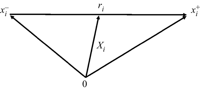
For inhomogeneous flows, we can formulate the problem only in real space using the generalised Kármán–Howarth equation. This is a balance equation for the second-order structure function and is formulated in a six-dimensional space, which comprises both the physical and scale spaces. The second-order structure function is defined locally at a point  $X_i$ in physical space, using the square of the difference between the fluctuating velocities at two points,
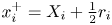 $x_i^+=X_i+\frac {1}{2}r_i$ and
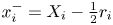 $x_i^-=X_i-\frac {1}{2}r_i$. This can be thought of as the energy of eddies with size smaller than
 $r=|r_i|$; refer to Davidson (Reference Davidson2015) for more details (and the caveats of this interpretation for eddies with size much smaller than
 $r$ and close to dissipation scales).
The equation was first derived for homogeneous isotropic turbulence by de Kármán & Howarth (Reference de Kármán and Howarth1938) using the two-point velocity correlation tensor. Later Kolmogorov (Reference Kolmogorov1941) reformulated the equation in terms of structure functions and proved the famous  $-4/5$ law that links the interscale energy flux, the separation between the two points and the dissipation rate. Under homogeneous isotropic turbulence conditions, this flux is always negative, indicating forward cascade, i.e. energy is transferred from large to small scales. The advantage of this equation is that even for homogeneous isotropic turbulence, it is expressed in spatial variables, rather than wavenumbers. This feature allows for generalisation to more complex flows, which includes the effect of anisotropy, shear and convection due to mean flow (Monin & Yaglom Reference Monin and Yaglom1975; Antonia et al. Reference Antonia, Ould-Rouis, Anselmet and Zhu1997, Reference Antonia, Zhou, Danaila and Anselmet2000; Danaila et al. Reference Danaila, Anselmet, Zhou and Antonia2001, Reference Danaila, Krawczynski, Thiesset and Renou2012; Danaila, Anselmet & Zhou Reference Danaila, Anselmet and Zhou2004).
The most general form of the equation appears in Hill (Reference Hill2002). For a weak formulation, which is more suitable for non-smooth, i.e. rough, velocity fields, see Duchon & Robert (Reference Duchon and Robert2000) and Dubrulle (Reference Dubrulle2019). The equation is derived directly from the Navier–Stokes equation applied at points  $x_i^+$ and
 $x_i^-$ and contains all the mechanisms that determine the evolution of the second-order structure function, i.e. how the energy at a particular scale is affected by production, dissipation and transfer in the physical
 $X_i$ and scale
 $r_i$ spaces. It does not make the assumptions of homogeneity and/or isotropy, and is thus suitable for our purposes. We note that in the limit of very large separations
 $r$, the Kármán–Howarth–Monin–Hill (KHMH) equation tends to the TKE (more precisely, it tends to twice the sum of the TKEs at points
 $x_i^+$ and
 $x_i^-$; see more details in § 3).
This equation has been applied extensively to fully developed, wall-bounded turbulent flows. It was employed for the first time by Marati, Casciola & Piva (Reference Marati, Casciola and Piva2004) to a low-Reynolds-number channel flow. The results showed that the well-known zonal decomposition of the flow in viscous layer, buffer region, logarithmic layer and bulk region is also meaningful in the context of a scale-by-scale budget. Saikrishnan et al. (Reference Saikrishnan, De Angelis, Longmire, Marusic, Casciola and Piva2012) studied the effect of Reynolds number in the range  $Re_\tau =180\text {--}934$ on the scale energy balance, while Cimarelli & De Angelis (Reference Cimarelli and De Angelis2012) focused on
 $Re_\tau =300$ and investigated in particular the inverse cascade for length scales larger than a cut-off value, and the associated difficulties for large-eddy simulation subgrid-scale modelling if the filter size is larger than this value. Visualisation of the scale energy flux in a three-dimensional hyper-plane (Cimarelli, De Angelis & Casciola Reference Cimarelli, De Angelis and Casciola2013) revealed spiral-like paths that originate from two energy sources, one located close to the wall (inner region) and the other further away (outer region). In Cimarelli et al. (Reference Cimarelli, De Angelis, Schlatter, Brethouwer, Talamelli and Casciola2015) particular attention was paid to the dynamics of the outer source, while in Cimarelli et al. (Reference Cimarelli, De Angelis, Jimenez and Casciola2016) the role of attached eddies on sustaining a reverse cascade towards the bulk flow was studied. More recently, Gatti et al. (Reference Gatti, Chiarini, Cimarelli and Quadrio2020) considered the balance equations for all components of the second-order structure function tensor and the interactions via the pressure-strain term.
The preceding short review has focused on attached wall-bounded flows as more relevant to the subject of this paper, but the equation has been applied to several other inhomogeneous and anisotropic flows, such as the near wake behind a square prism (Alves Portela, Papadakis & Vassilicos Reference Alves Portela, Papadakis and Vassilicos2017, Reference Alves Portela, Papadakis and Vassilicos2020), von Kármán flows (Dubrulle Reference Dubrulle2019; Knutsen et al. Reference Knutsen, Baj, Lawson, Bodenschatz, Dawson and Worth2020), planar jets (Cimarelli et al. Reference Cimarelli, Mollicone, Van Reeuwijk and De Angelis2021) and the recirculating flow behind a bump (Mollicone et al. Reference Mollicone, Battista, Gualtieri and Casciola2018).
The success of the KHMH equation in describing the complex interscale dynamics of near-wall turbulence justifies the adoption of this framework to explore similar issues in bypass transition. As explained earlier, the equation is very general, and therefore applicable in laminar, transitional and fully turbulent regimes. Thus, it can be employed across the laminar–turbulent interface, allowing us to get a unique glimpse of the interscale energy transfer process in transitional flows.
The paper is organised as follows. In § 2 the flow conditions for the case considered are briefly described and comparisons against reference data from the literature are presented. In § 3 we introduce the KHMH equation, while in §§ 4 to 7 scale energy fluxes in two-dimensional planes and three-dimensional hyper-planes are presented and discussed. In § 8 we relate the observed fluxes with the instantaneous flow fields (that contain laminar regions and turbulent patches) and investigate their probability density functions (PDFs). We conclude in § 9.
2. Test case details and one-point statistics
We consider the transitional flow in a flat-plate boundary layer. The turbulence intensity in the free stream is set to 3.4 %, and the fluctuations are assumed to follow a von Kármán spectrum. Spatial coordinates are normalised by the Blasius similarity variable  $L_0 = \sqrt {\nu X_0/U_\infty }$, where
 $X_0$ is the distance of the domain inlet from the leading edge of the plate,
 $U_\infty$ is the free-stream velocity and
 $\nu$ the kinematic viscosity of the fluid. The integral length scale of free-stream turbulence is set to
 $L_{11}=5L_0$, which is approximately equal to the boundary layer thickness at the inlet. The Reynolds number based on the Blasius similarity variable is
 $Re_{L_0}=160$ (or
 $Re_{\theta }=110$ based on momentum thickness). The computational domain in the streamwise (
 $X$), wall-normal (
 $Y$) and spanwise (
 $Z$) directions is
 $3000\times 200\times 150$. This domain is discretised using
 $2049\times 192\times 169$ cells in the
 $X$,
 $Y$ and
 $Z$ directions, respectively. The grid spacings in wall units are
 $\Delta x^{+}_{max}\approx 11.78$,
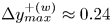 $\Delta y^{+(w)}_{max}\approx 0.24$ and
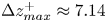 $\Delta z^{+}_{max}\approx 7.14$. The subscript
 ${max}$ denotes maximum values in the fully turbulent region, while
 $\Delta y^{+(w)}_{max}$ is evaluated at the centroid of the first cell close to the wall.
We employ a previously generated direct numerical simulation database for the aforementioned conditions; refer to Yao, Alves-Portela & Papadakis (Reference Yao, Alves-Portela and Papadakis2020) for details regarding generation of inlet conditions, numerical schemes in space and time, order of accuracy, Courant–Friedrichs–Lewy numbers, etc. The database comprises 350 instantaneous snapshots of the flow. The time separation between two snapshots is  $20T_0$, where
 $T_0=L_0/U_\infty$. To increase the number of samples and improve convergence of the statistics, we perform both time and spanwise averaging.
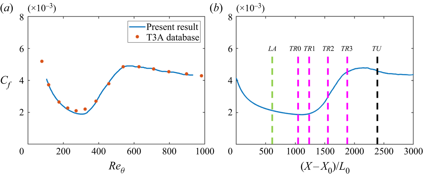
Figure 1 shows the variation of the friction coefficient  $C_f$ as the flow transitions from laminar to turbulent. The results match well with the experiments of the T3A database (Roach Reference Roach1990). Note that in the experiment, the free-stream turbulence intensity is set to
 $3.3\,\%$; however, in the current simulation,
 $3.4\,\%$ is used (as already mentioned) in order to match the transition onset. We study the spatial evolution of the interscale energy fluxes at six locations, placed in the laminar
 $(LA)$, transitional
 $(TR0,TR1,TR2,TR3)$ and fully turbulent
 $(TA)$ regions; these locations are shown in figure 1(b).
Skin friction coefficient  $C_f$ against
 $Re_{\theta }$ (a) and distance from the inlet of the domain
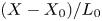 $(X-X_0)/L_0$ (b). The green and black vertical lines denote locations at the laminar
 $(LA)$ and turbulent
 $(TU)$ regions, respectively. The purple vertical lines denote four stations
 $TR0,TR1,TR2,TR3$ within the transitional region. The coordinates are
 $(X-X_0)/L_0=540,1065,1215,1515,1815$ and
 $2415$ for
 $LA,TR0,TR1,TR2,TR3$ and
 $TU$, respectively.

Before we proceed to examine the evolution of two-point statistics using the KHMH equation, it is instructive to examine first the budgets of the TKE equation,
 \begin{align} \underbrace{\frac{\partial (U_i k)}{\partial x_i}}_{\text{convection}(\mathcal{A}_k)} &= \underbrace{-\langle u_i u_j \rangle \frac{\partial U_j}{\partial x_i}}_{\text{production} (\mathcal{P}_k)} - \underbrace{\nu \left\langle \frac{\partial u_j}{\partial x_i} \frac{\partial u_j}{\partial x_i} \right\rangle }_{\text{dissipation} (\epsilon_k)} \nonumber\\ &\quad +\underbrace{ \frac{\partial}{\partial x_i} \left(\nu \frac{\partial k}{\partial x_i}\right)}_{\text{viscous diffusion} (\mathcal{D}_k)} \underbrace{- \frac{\partial}{\partial x_i} \left(\frac{1}{2}\langle u_i u_j u_j \rangle \right)}_{\text{turbulent diffusion} (\mathcal{T}_k)} \underbrace{- \frac{\partial}{\partial x_i} \left(\frac{1}{\rho} \langle u_i p \rangle \right)}_{\text{pressure diffusion} (\mathcal{T}_{p,k})}, \end{align}
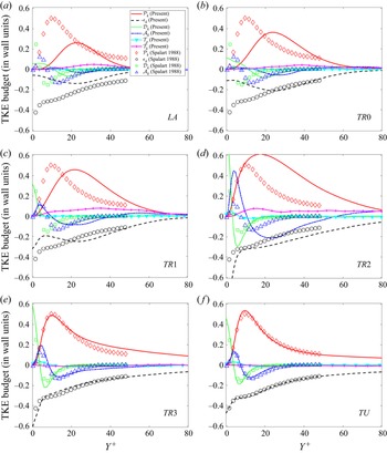
at these six locations. Figure 2 shows the evolution of the budget terms plotted against the distance from the wall for all streamwise positions; variables are normalised using the local wall units. The open symbols represent the reference direct numerical simulation data of Spalart (Reference Spalart1988) and are repeated in every panel. The matching between the present results at the  $TU$ region (where
 $Re_{\theta }=800$) and the reference data (where
 $Re_{\theta }=1410$) is very good for all terms. This provides further evidence of the validity of the generated database. Comparison between the lines and symbols indicates the deviation from the fully turbulent state at each location.
The TKE budgets at locations (a)  $LA$, (b)
 $TR0$, (c)
 $TR1$, (d)
 $TR2$, (e)
 $TR3$ and (f)
 $TU$. The symbols represent data from Spalart (Reference Spalart1988) for
 $Re_{\theta }=1410$.
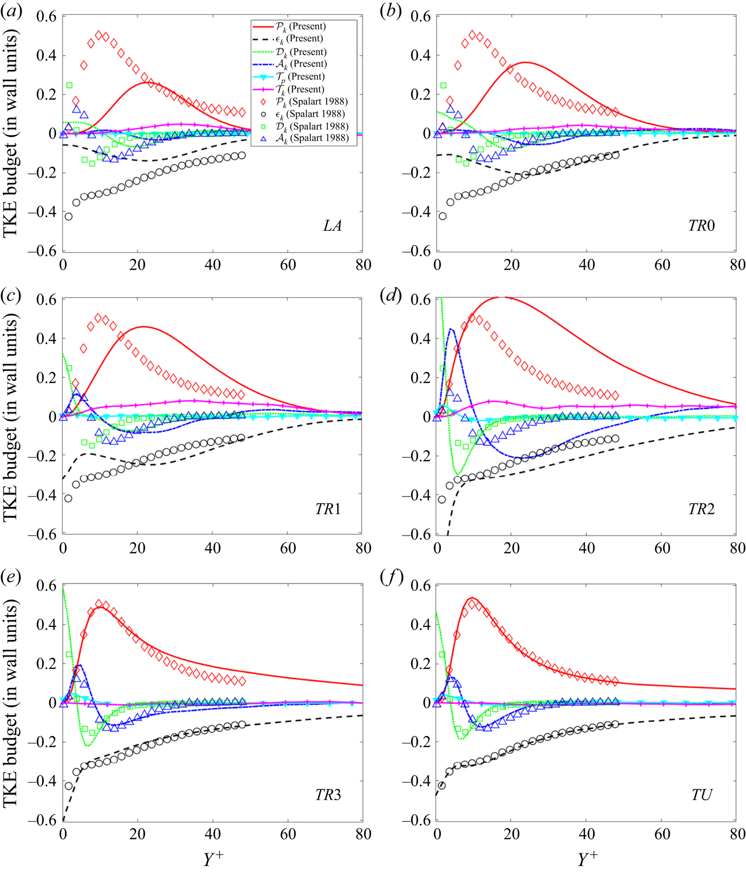
In the laminar regime (figure 2a), where the boundary layer is distorted by Klebanoff modes, the production term has an approximately symmetric shape, peaks at  $Y^+\approx 21$ and reaches a relatively small value. As the flow transitions, the production peak grows, moves closer to the wall and finally settles at
 $Y^+ \approx 16$ (figure 2f), i.e. in the buffer layer. A production overshoot appears at
 $TR2$, which is in the middle of the transition region. At this position the maximum intermittency is about
 $40\,\%$ (refer to figure 4 of Yao et al. (Reference Yao, Alves-Portela and Papadakis2020)) and grows fast indicating the rapid formation and growth of turbulent spots. Nolan & Zaki (Reference Nolan and Zaki2013) report an overshoot in the streamwise root-mean-square velocity in exactly the same position, i.e. when the skin friction is midway between the laminar and turbulent values.
At  $LA$, dissipation peaks within the Klebanoff mode core, but further downstream the maximum value grows, and beyond
 $TR1$ it settles at the wall, where it is balanced by viscous diffusion, as expected. Turbulent diffusion has small contribution at
 $LA$,
 $TR0$ and
 $TR1$, but becomes very significant at
 $TR2$, with a sharp positive peak close to the wall at
 $Y^+ \approx 5$ and a shallower negative trough at
 $Y^+ \approx 22$. At this location, three terms dominate for
 $Y^+>15$: production, dissipation and turbulent diffusion. Note also the very sharp rise of dissipation close to the wall, and the important contribution of turbulent diffusion to balance it. Further downstream, at
 $TR3$ and
 $TU$, all terms settle to smaller values.
The largest deviation from equilibrium, quantified by the difference between production and dissipation for  $Y^+ > 15$, appears in
 $TR2$; this is the position with the largest growth of
 $C_f$ as evidenced in figure 1, consistent with the rapid increase of intermittency, as mentioned earlier. At
 $TR3$, where
 $C_f$ starts to stabilise marking the end of transition, the budgets are very similar to those at the fully turbulent state,
 $TU$. In the latter state turbulence is in equilibrium, with production balancing dissipation for
 $Y^+ > 25$. In all locations the convection term plays a minor role. It becomes more important in
 $TR2$ (and less so in
 $TR1$) for
 $Y^+ > 60$, where it balances production, dissipation and turbulent diffusion.
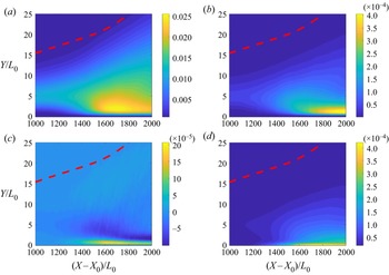
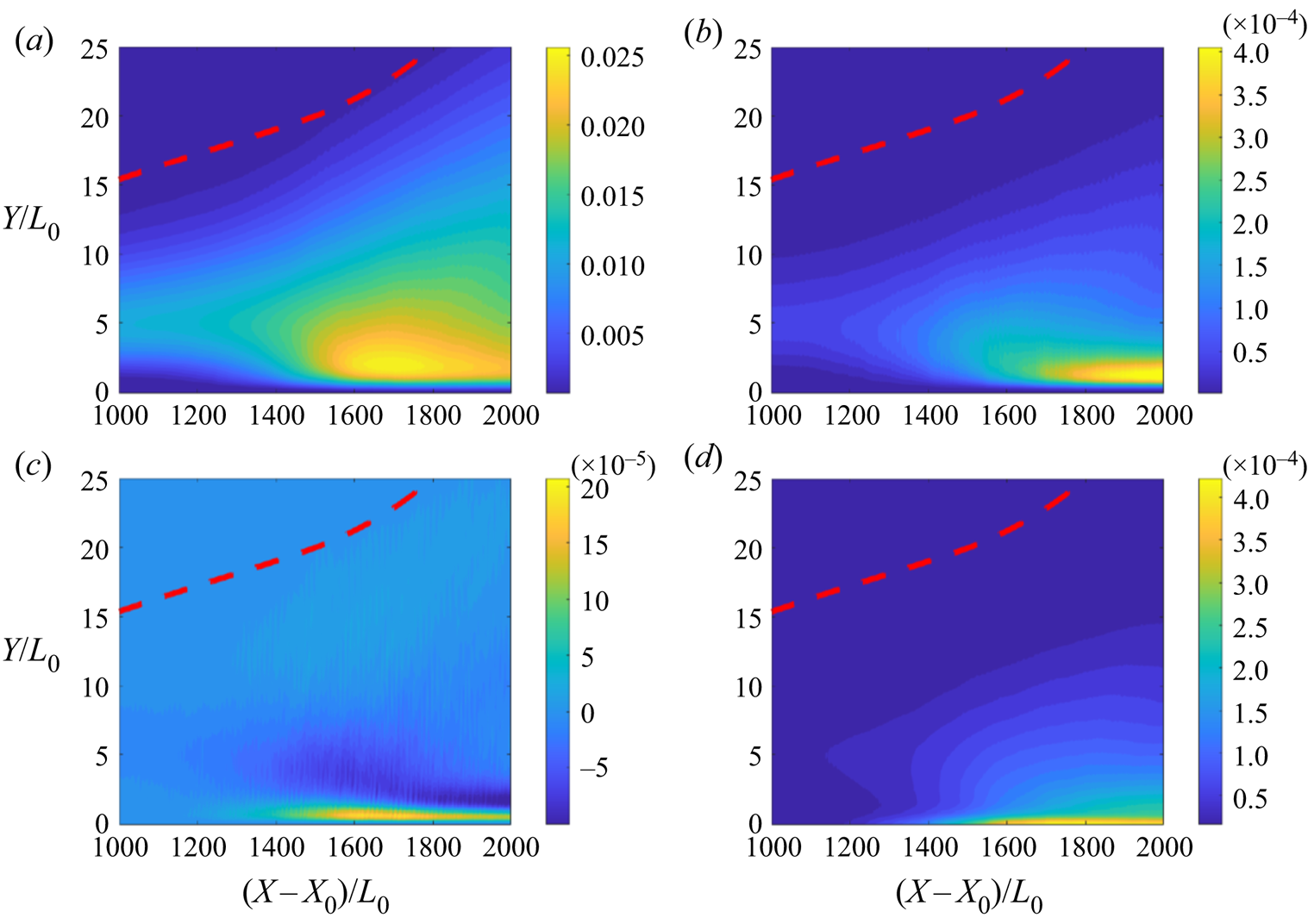
The strong wall-normal and streamwise inhomogeneity are more clearly demonstrated in the contour plots of TKE, production, turbulent transport and dissipation shown in figure 3, where all terms are normalised by global variables (free-stream velocity  $U_\infty$ and Blasius variable at the inlet
 $L_0$). Turbulent kinetic energy and turbulent transport peak at
 $(X-X_0)/L_0 \approx 1650$, slightly downstream of
 $TR2$. When normalised with global variables, the production term reaches maximum in the turbulent regime. The peak of TKE therefore at
 $(X-X_0)/L_0 \approx 1650$ arises from the strong positive value of turbulent transport close to the wall (yellow region in figure 3c). Dissipation grows sharply downstream of
 $(X-X_0)/L_0 \approx 1600$ and is maximised at the wall.
Contour plots of (a) TKE, (b) production, (c) turbulent diffusion and (d) dissipation. All variables are normalised with global units. The red dashed line indicates the location of the boundary layer thickness.
The TKE is a one-point equation and energy is transported only in physical space. In the next section we look at the transport of energy in both physical and scale spaces using the KHMH equation.
3. Two-point KHMH equation
The KHMH equation is a balance equation for the second-order structure function, defined as  $\delta q^2=(\delta u_i)^2=(u_i^+-u_i^-)^2$, where
 $u_i^+$ and
 $u_i^-$ are the velocity fluctuations around the time averages
 $U_i^+$ and
 $U_i^-$ at two points
 $x_i^+$ and
 $x_i^-$, respectively (refer to figure 4). Denoting the midpoint as
 $X_i=0.5(x_i^++x_i^-)$ and the separation between the two points as
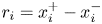 $r_i=x_i^+-x_i^-$, it is evident that for a general three-dimensional inhomogeneous and anisotropic flow,
 $\delta q^2$ is a function of three spatial and three separation (or scale) variables, i.e.
 $\delta q^2(X_i,r_i)$. Using angular brackets to represent time averages, the transport equation of
 $\langle \delta q^2(X_i,r_i) \rangle$ takes the form (Hill Reference Hill2002)
 \begin{align} &\underbrace{\dfrac{\partial \langle \delta q^2 \rangle}{\partial t}}_ {\substack{\text{Transient} \\ \text{term ($\mathcal{A}_t$)}}} + \underbrace{\dfrac{\partial \dfrac{(U_i^+{+} U_i^-)}{2} \langle \delta q^2 \rangle}{\partial X_i}}_{\text{Mean flow advection} (\mathcal{A}_U)} + \underbrace{\dfrac{\partial \langle \delta u_i \delta q^2 \rangle}{\partial r_i}}_ {\substack{\text{Nonlinear interscale } \\ \text{transfer ($\varPi$)}}} + \underbrace{\dfrac{\partial \delta U_i \langle \delta q^2 \rangle}{\partial r_i}}_ {\substack{\text{Linear interscale } \\ \text{transfer ($\varPi_U$)}}}\nonumber\\ &\quad = \underbrace{- \dfrac{\partial\left \langle \dfrac{(u_i^+{+} u_i^-)}{2} \delta q^2 \right\rangle}{\partial X_i}}_ {\substack{\text{Turbulent} \\ \text{advection ($\mathcal{A}_u$)}}} \underbrace{- 2\dfrac{\partial \langle \delta u_i \delta p \rangle}{\partial X_i}}_{\substack{\text{Pressure-velocity} \\ \text{correlation ($\mathcal{T}_p$)}}} + \underbrace{ \dfrac{1}{2} \nu \dfrac{\partial^2 \langle \delta q^2 \rangle}{\partial X_i \partial X_i}}_ {\substack{\text{Diffusion in physical} \\ \text{space ($\mathcal{D}_x$)}}} \nonumber\\ &\qquad + \underbrace{2\nu \dfrac{\partial^2 \langle \delta q^2 \rangle}{\partial r_i \partial r_i}}_ {\substack{\text{Diffusion in scale} \\ \text{space ($\mathcal{D}_r$)}}} \underbrace{- 2\langle \delta u_i \delta u_j \rangle \dfrac{\partial \delta U_j}{\partial r_i} - \langle (u_i^+{+} u_i^-)\delta u_j \rangle \dfrac{\partial \delta U_j}{\partial X_i}}_{\text{Production by mean flow} (\mathcal{P})}\nonumber\\ &\qquad -\underbrace{ 4\nu \left( \dfrac{1}{4}\left\langle \dfrac{\partial \delta u_j}{\partial X_i} \dfrac{\partial \delta u_j}{\partial X_i} \right\rangle + \left\langle \dfrac{\partial \delta u_j}{\partial r_i} \dfrac{\partial \delta u_j}{\partial r_i} \right\rangle \right)}_{\text{Dissipation}(\epsilon)} . \end{align}
Schematic of the points  $x_i^+$ and
 $x_i^-$ used to define
 $\delta q^2$, the midpoint
 $X_i$ and the separation vector
 $r_i$.

As noted in the introduction,  $\langle \delta q^2 \rangle$ can be interpreted as the energy of eddies with size smaller than
 $r=|r_i|$. For statistically steady flows, as the ones considered in the present paper, the transient term
 $\mathcal {A}_t=0$. Defining
 $U_i^*=({U_i^+ + U_i^-})/{2}$ and
 $u_i^*=({u_i^+ + u_i^-})/{2}$ as the midpoint values of the mean and fluctuating velocities, respectively, and grouping together the terms computed in physical (
 $X_i$) and scale (
 $r_i$) spaces, (3.1) can be rearranged as
 \begin{align} &\underbrace{\dfrac{\partial \left[ \langle U_i^*\delta q^2 \rangle \!+\! \langle u_i^* \delta q^2 \rangle \!+\! \langle 2 \delta u_i \delta p \rangle - \dfrac{1}{2} \nu \dfrac{\partial \langle \delta q^2 \rangle}{\partial x_i}\right] }{\partial X_i}}_{\text{Transport in physical space}} + \underbrace{\dfrac{\partial \left[\langle \delta u_i \delta q^2 \rangle \!+\! \langle \delta U_i \delta q^2 \rangle - 2\nu \dfrac{\partial \langle \delta q^2 \rangle}{\partial r_i}\right]}{\partial r_i}}_{\text{Transport in scale space}}\nonumber\\ &\quad = \underbrace{- 2\langle \delta u_i \delta u_j \rangle \dfrac{\partial \delta U_j}{\partial r_i} - 2\langle u_i^* \delta u_j \rangle \dfrac{\partial \delta U_j}{\partial X_i}}_{\text{Production}} -\underbrace{ 4\nu \left( \dfrac{1}{4}\left\langle \frac{\partial \delta u_j}{\partial X_i} \frac{\partial \delta u_j}{\partial X_i} \right\rangle + \left\langle \frac{\partial \delta u_j}{\partial r_i} \frac{\partial \delta u_j}{\partial r_i} \right\rangle \right)}_{\text{Dissipation}} . \end{align}
This form is more useful because the transport terms are now written as the divergence of fluxes in the two spaces. Indeed, we can rewrite (3.2) in a compact form as
 \begin{equation} \frac{\partial \boldsymbol{{\phi_s}_i} }{\partial X_i} + \frac{\partial \boldsymbol{{\phi_r}_i}}{\partial r_i} = \mathcal{P} -\epsilon \equiv \mathcal{P}_{net}, \end{equation}
and define

as the flux vector in physical space and

as the flux vector in scale space. As before,
 \begin{equation} \mathcal{P}={-} 2\langle \delta u_i \delta u_j \rangle \frac{\partial \delta U_j}{\partial r_i} - 2\langle u_i^* \delta u_j \rangle \frac{\partial \delta U_j}{\partial X_i} \end{equation}
is the production term and
 \begin{equation} \epsilon= 4\nu \left( \frac{1}{4}\left\langle \frac{\partial \delta u_j}{\partial X_i} \frac{\partial \delta u_j}{\partial X_i}\right\rangle + \left\langle \frac{\partial \delta u_j}{\partial r_i} \frac{\partial \delta u_j}{\partial r_i} \right \rangle \right)=2\left(\epsilon^+{+} \epsilon^-\right)=4\epsilon^* \end{equation}
is the dissipation term. In the above equation,  $\epsilon ^+=\nu \langle ({\partial u_j^+}/{\partial x_i^+})({\partial u_j^+}/{\partial x_i^+})\rangle$ and
 $\epsilon ^-=\nu \langle ({\partial u_j^-}/{\partial x_i^-})({\partial u_j^-}/{\partial x_i^-})\rangle$ are the local dissipations at points
 $x_i^+$ and
 $x_i^-$, respectively, while
 $\epsilon ^*=({\epsilon ^+ + \epsilon ^-})/{2}$ is the midpoint value. Note that in (3.3) we have also defined the net production as
 $\mathcal {P}_{net}=\mathcal {P} -\epsilon =\mathcal {P}-4\epsilon ^*$.
In (3.4) and (3.5) we have decomposed the flux vectors into constituent components due to mean flow, turbulent fluctuations, pressure and viscous diffusion; these are denoted with superscripts  $\boldsymbol {M}$,
 $\boldsymbol {F}$,
 $\boldsymbol {P}$ and
 $\boldsymbol {V}$, respectively, i.e.
 $\boldsymbol {\phi _s} = \boldsymbol {\phi ^M_{s}}+ \boldsymbol {\phi ^F_{s}}+ \boldsymbol {\phi ^V_{s}}+ \boldsymbol {\phi ^P_{s}}$ and
 $\boldsymbol {\phi _r} = \boldsymbol {\phi ^M_{r}}+ \boldsymbol {\phi ^F_{r}}+ \boldsymbol {\phi ^V_{r}}$. In summary, we have four flux vector pairs arising from different mechanisms:
 $(\boldsymbol {\phi ^M_{s}},\boldsymbol {\phi ^M_{r}})$,
 $(\boldsymbol {\phi ^F_{s}},\boldsymbol {\phi ^F_{r}})$,
 $(\boldsymbol {\phi ^V_{s}},\boldsymbol {\phi ^V_{r}})$,
 $(\boldsymbol {\phi ^P_{s}},0)$. Note that if we define
 $p^*=({p^+ + p^-})/{2}$ as the midpoint value of the fluctuating pressure, it is easy to prove that
 $2({\partial \langle \delta u_i \delta p \rangle }/{\partial X_i})=8({\partial \langle \delta u_i p^* \rangle }/{\partial r_i})$, so the pressure–velocity correlation term can be written in flux divergence form in either physical or scale space (here we write this term in physical space).
It is possible to write (3.3) in an even more compact form as
 \begin{equation} \frac{\partial \boldsymbol{{\phi_\xi}_i} }{\partial \xi_i} = \mathcal{P}-4\epsilon^*, \end{equation}
where  $\xi =(x_1,x_2,x_3,r_1,r_2,r_3)$ is the composite position vector and
 $\boldsymbol {\phi _\xi }(\xi )=({{\phi _s}_1},{{\phi _s}_2},{{\phi _s}_3},{{\phi _r}_1},{{\phi _r}_2},{{\phi _r}}_3)$ is a six-dimensional flux vector, with each component depending on
 $\xi$.
In the flow considered in this paper, only the spanwise direction  $x_3$ is homogeneous, so averaging is performed in time and along
 $x_3$. The composite position vector
 $\xi$ and the flux vector
 $\boldsymbol {\phi _\xi }(\xi )$ thus become five-dimensional, i.e.
 \begin{equation} \xi=(x_1,x_2,r_1,r_2,r_3) \quad \mbox{and} \quad \boldsymbol{\phi_\xi}(\xi)=({\phi_s}_1,{\phi_s}_2,{\phi_r}_1,{\phi_r}_2,{\phi_r}_3). \end{equation}
Due to this high dimensionality judicious choices must be made in the selection of the projection hyper-planes that will allow the extraction of the maximum amount of information. In the present paper, we project the flux vector to the two-dimensional planes  $(r_3,x_2=Y)$,
 $(r_1,x_2=Y)$ and the three-dimensional hyper-plane
 $(r_1,r_3,x_2=Y)$, i.e. we plot
 $({{\phi _r}_3},{{\phi _s}_2})$,
 $({{\phi _r}_1},{{\phi _s}_2})$ and
 $({{\phi _r}_1},{{\phi _r}_3},{{\phi _s}_2})$ at several streamwise locations
 $x_1$. For all cases, we have assumed that the separation in the wall-normal direction is
 $r_2=0$.
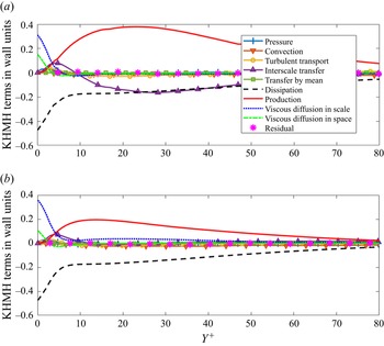
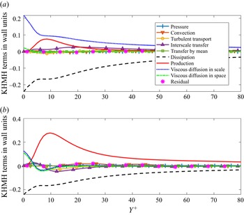
In the Appendix we provide evidence that the computed fields balance the KHMH equation. In figures 18 and 19 we plot the variation of the budget terms in the wall-normal direction for two streamwise locations,  $TR2$ and
 $TU$, and two pairs of separations. As can be seen, the equation is balanced very well; the residual is at most a few percentage points of maximum production. Similar results were found for other locations and streamwise/spanwise separations.
We close this section by mentioning that as the separation increases, i.e.  $\lvert r_i \rvert \to \infty$, the velocity correlation
 $\langle u_i^+u_i^- \rangle \to 0$ and therefore
 $\langle \delta q^2 \rangle \to 2 (k^++k^-)$, where
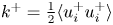 $k^+=\frac {1}{2}\langle {u_i^+}{u_i^+} \rangle$ and
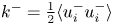 $k^-=\frac {1}{2}\langle {u_i^-}{u_i^-} \rangle$ are the TKEs at points
 $x_i^+$ and
 $x_i^-$, respectively. Thus for large separations, the asymptotic form of (3.2) is twice the sum of the TKE transport equations (2.1) applied at each point. Both the nonlinear interscale transfer
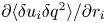 ${\partial \langle \delta u_i \delta q^2 \rangle }/{\partial r_i}$ and the turbulent advection
 ${\partial \langle ({(u_i^+ + u_i^-)}/{2}) \delta q^2 \rangle }/{\partial X_i}$ tend to
 \begin{equation} \frac{1}{2} \left( \frac{\partial}{\partial x_i^+}\langle u_i^+ u_j^+ u_j^+ \rangle + \frac{\partial}{\partial x_i^-}\langle u_i^- u_j^- u_j^- \rangle\right) \end{equation}
as  $\lvert r_i \rvert \to \infty$, thus both contribute equally to the turbulent diffusion term of the TKE equation.
4. Energy fluxes on the  $(r_3,Y)$ plane

4.1. General characteristics
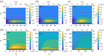
Figure 5 shows the evolution of the flux vector components  $(\boldsymbol {{\phi _r}_3},\boldsymbol {{\phi _s}_2})$ in the
 $(r_3,Y)$ plane (with
 $r_1=0$) from the laminar to turbulent region. Wall-normal distances and separations are normalised by the local wall variables (left and bottom axes) and global variables (top and right axes). The pink dashed line indicates the local boundary layer thickness. In order to facilitate the interpretation of these plots, we also superimpose coloured contours of the net production,
 $\mathcal {P}_{net}=\mathcal {P}-\epsilon$.
(a–f) Evolution of energy flux vector  $(\boldsymbol {{\phi _r}_3},\boldsymbol {{\phi _s}_2)}$ on
 $(r_3, Y)$ plane (red arrows) from laminar to turbulent region. The coloured contour is the net production (normalised with global variables) and the pink dashed lines indicate the local boundary layer thickness. The yellow arrows in (d) point to the two sink regions,
 $r_3=0$ and
 $Y=0$. The maximum vector magnitude (corresponding to the longest arrow on each plot) is
 $5\times 10^{-5}, 7.6\times 10^{-5}, 9.1\times 10^{-5}, 1.7\times 10^{-4}, 2.4\times 10^{-4}, 2.2\times 10^{-4}$ from
 $LA$ to
 $TU$, respectively.

At all spatial locations  $\mathcal {P}_{net}$ peaks at particular
 $r_3$ separations and wall-normal distances
 $Y$ (the peaks appear as concentrated yellow regions). The production
 $\mathcal {P}$ arises from the inhomogeneity of the time-average flow in the physical and scale spaces, as evidenced by the two terms in (3.6). We analysed the contribution of each term and found that the large production arises due to the inhomogeneity in scale space, and in particular from the component
 $-2\langle \delta u_2 \delta u_1 \rangle {\partial \delta U_1}/{\partial r_2}\vert _{r_2=0}$. The contribution of the second term is exactly 0 (due to the spanwise homogeneity of the time-average flow). It is easier to understand the physical mechanism that leads to high production if we focus on the laminar region (figure 5a). In this region Klebanoff modes (laminar streaks) are present that result in positive and negative streamwise velocity fluctuations; therefore
 $\delta u_1$ is maximised when
 $r_3$ is equal to the distance between two streaks. The wall-normal fluctuation differences
 $\delta u_2$ are also maximised at the same distance (refer to figure 24 in Xiao & Papadakis (Reference Xiao and Papadakis2019)) resulting in large time and spanwise averages
 $\langle \delta u_2 \delta u_1 \rangle$. The shear rate in scale space can be written as
 \begin{equation} \frac{\partial \delta U_1}{\partial r_2}=\frac{1}{2}\left(\frac{\partial \delta U_1}{\partial x_2^+}-\frac{\partial \delta U_1}{\partial x_2^-} \right)= \frac{1}{2}\left(\frac{\partial U_1^+}{\partial x_2^+}+\frac{\partial U_1^-}{\partial x_2^-} \right) \end{equation}
and due to spanwise homogeneity of  $U_1$ and the fact that
 $r_2=0$ (meaning that
 $x_2^+=x_2^-=x_2=Y$, thus
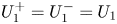 $U_1^+=U_1^-=U_1$) this can be simplified to
 ${\partial \delta U_1}/{\partial r_2}\vert _{r_2=0}={\partial U_1}/{\partial x_2}$. The production term can therefore be written as
 $\mathcal {P} = -2\langle \delta u_2 \delta u_1 \rangle {\partial U_1}/{\partial x_2}$. The corresponding term for the TKE equation is
 $\mathcal {P}_k \approx -\langle u_2 u_1 \rangle {\partial U_1}/{\partial x_2}$, which is of course uniform in the spanwise direction (see figure 3b). The peak production location of the KHMH equation in the
 $(r_3,Y)$ plane is therefore determined by the spanwise distance between the Klebanoff modes and the wall-normal distance at which the product of the second-order structure function
 $\langle \delta u_2 \delta u_1 \rangle$ and the shear
 ${\partial U_1}/{\partial x_2}$ is maximum. The mean flow therefore injects energy at a specific
 $r_3$ separation, which is determined by the receptivity process arising from the interaction between free-stream turbulence forcing and shear during the early development of the boundary layer. This process controls the spacing between the Klebanoff modes, which is of the order of the boundary layer thickness close to the inlet.
As the flow evolves, the location of peak net production changes smoothly and approaches the wall. The largest energy production appears at the  $TU$ location, inside the buffer layer, at
 $Y^+\approx 12$ and
 $r_3^+ \approx 40$, consistent with the results of Cimarelli et al. (Reference Cimarelli, De Angelis, Schlatter, Brethouwer, Talamelli and Casciola2015) for channel flow. The large production at specific regions in the
 $(r_3,Y)$ plane strongly affects the energy transfer in the physical and scale spaces, to which we now turn.
For all streamwise locations the energy fluxes originate from the  $\mathcal {P}_{net}$ peak location and radiate outwards. In the laminar region (
 $LA$), most of the energy produced flows to smaller
 $r_3$ scales and is dissipated (forward cascade). There is weak inverse cascade to larger
 $r_3$ scales, while the energy flux in the wall-normal direction is negligible. At the turbulent region (
 $TU$) the fluxes show a different behaviour. The energy injected from the time-average flow radiates in all directions. There are two sinks indicated by yellow arrows in the
 $TR2$ plot of figure 5; one towards the wall (where it is dissipated) and the other towards small
 $r_3$ scales (indicating a forward cascade). An inverse energy cascade also appears, i.e. energy flows to larger
 $r_3$ scales to the right of the
 $\mathcal {P}_{net}$ before most of the flux vectors then change direction and bend towards the
 $Y$ axis (
 $r_3=0$). This map is very similar to that of turbulent channel flow (Cimarelli et al. Reference Cimarelli, De Angelis and Casciola2013, Reference Cimarelli, De Angelis, Schlatter, Brethouwer, Talamelli and Casciola2015, Reference Cimarelli, De Angelis, Jimenez and Casciola2016).
In the transition region, the scale energy transfer pattern morphs progressively from laminar to turbulent shape. Downstream of  $TR0$, the energy flux in the wall-normal direction (i.e. towards the bulk of the flow) energises the region above the Klebanoff modes, increasing the thickness of the boundary layer. This indicates that the equilibrium boundary layer at
 $TU$ is forming gradually during the transition process. Significant inverse cascade appears towards larger
 $r_3$ scales, but it is noteworthy that the bending of the energy flux vectors towards small scales does not appear in the transition region, but only at the
 $TU$ region. It seems that strong inverse cascade is a central characteristic of transition; we will elaborate more on this important feature again later.
In order to shed more light onto the patterns shown in figure 5, we turn our attention to the decompositions (3.4) and (3.5) and investigate the contributions of fluxes due to mean flow, nonlinear interactions, viscosity and pressure.
4.2. Analysis of decomposed energy fluxes
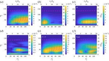
We focus in particular on the  $TR2$ location, in the middle of the transition region. In figure 6 we plot the four pairs of fluxes
 $(\boldsymbol {\phi ^F_{r_3}},\boldsymbol {\phi ^F_{s_2}})$,
 $(\boldsymbol {\phi ^V_{r_3}},\boldsymbol {\phi ^V_{s_2}})$,
 $(\boldsymbol {\phi ^M_{r_3}},\boldsymbol {\phi ^M_{s_2}})$ and
 $(\boldsymbol {0,\phi ^P_{s_2}})$ in the
 $(r_3,Y)$ plane; these are denoted with F, V, M and P, respectively. We also plot the sum
 $( \boldsymbol {\phi ^F_{r_3}}+\boldsymbol {\phi ^V_{r_3}},\boldsymbol {\phi ^F_{s_2}}+\boldsymbol {\phi ^V_{s_2}})$, denoted as
 $\boldsymbol {F}+\boldsymbol {V}$, and the total flux
 $(\boldsymbol {{\phi _r}_3},\boldsymbol {{\phi _s}_2})$, which is of course identical to that shown in figure 5(d). In all plots, the flux vectors are plotted as arrows to show the direction, but we also superimpose the flux magnitude as contours.
Maps of flux vectors due to nonlinear interaction between (a) velocity fluctuations  $(F)$, (b) viscosity
 $(V)$, (c) mean velocity
 $(M)$, (d) pressure
 $(P)$, (e) combination
 $(F+V)$ and (f) total on
 $(r_3,Y)$ plane at
 $TR2$ location. Contours represent the magnitude of the corresponding flux vectors.

We first note that the fluxes due to mean flow and pressure have components only in physical space, i.e. the wall-normal direction; this is because  $\boldsymbol {\phi ^P_{r_3}}=0$ and
 $\boldsymbol {\phi ^M_{r_3}}=\langle \delta U_i \delta q^2 \rangle =0$ due to homogeneity in the spanwise direction. Therefore in the
 $r_3$ direction the fluxes are due to the nonlinear and viscous terms only,
 $\boldsymbol {\phi ^F_{r_3}}$ and
 $\boldsymbol {\phi ^V_{r_3}}$. The latter term results in forward cascade, while the former transfers energy to larger scales (inverse cascade) and to the bulk of the flow. The superposition of these two terms results in the
 ${\boldsymbol {F}}+{\boldsymbol {V}}$ pattern, which is almost identical to the total in the
 $r_3$ direction. Adding the contribution of pressure and mean flow terms, which both transfer energy towards the wall, readjusts the direction of the arrows, and completes the picture. The readjustment is especially evident at
 $Y \approx 5L_0$, and results in almost horizontal total inverse fluxes.
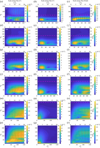
In figure 7 we plot the evolution of the two most important terms (viscous and nonlinear) at all streamwise locations. For comparison purposes, we also include the total flux in the same plot (right-hand column). We first notice that the viscous flux (middle column) results mainly in forward cascade (but there are some regions of very weak inverse cascade) and energy towards the wall. As transition progresses, the forward cascade acts at progressively smaller scales, while the energy transfer towards the wall becomes stronger. The latter is firmly established over a wide range of scales in the viscous sublayer when the turbulent region is reached. The viscous effect can be clearly seen also on the total energy flux plots, especially in the  $TR3$ and
 $TU$ locations. The energy transfer due to the nonlinear interaction term is more involved. This term mainly acts to transfer energy to larger scales (inverse cascade) and this is evident at all streamwise locations, even in the laminar (
 $LA$) region (but it is quite weak there). Starting from the
 $TR0$ location, it also acts to transfer energy to the bulk of the flow. The radial flux pattern that appears in the total flux plots (right-hand column) is thus due to the superposition of the effects of the nonlinear interaction and viscous terms.
Evolution of energy fluxes due to the nonlinear interaction term (a,d,g,j,m,p) and the viscous term (b,e,h,k,n,q) in the  $(r_3,Y)$ plane. (c,f,i,l,o,r) The total flux. Contours represent the magnitude of the corresponding flux vectors. The pink dashed line is the local boundary layer thickness.

We now turn our attention to energy transfer in the  $(r_1, Y)$ plane.
5. Energy fluxes on the $(r_1, Y)$ plane

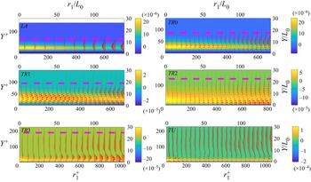
For each streamwise location, we select the  $r_3$ value that corresponds to the peak net production shown in figure 5; the resulting separations are
 $r_3/L_0=8,8,8,8,5,5$ at positions
 $LA,TR0,TR1,TR2,TR3,TU$, respectively. This allows us to investigate the behaviour of the energy fluxes at the particular
 $r_3$ separation at which the energy due the mean shear is injected.
5.1. General characteristics
Figure 8 shows the evolution of the energy flux vector  $(\boldsymbol {{\phi _r}_1}, \boldsymbol {{\phi _s}_2})$ on this plane. A core region of strong net production, indicated by yellow colour, can be clearly seen; this region persists throughout transition. At the
 $LA$ location, this region is concentrated at small
 $r_1$ values,
 $0< r_1/L_0<75$, but as transition progresses, it moves closer to the wall and it is elongated. Gradually, it occupies the whole range of
 $r_1$ separations considered,
 $0< r_1/L_0<150$. Note also that apart from the first two locations
 $LA$ and
 $TR0$, net production can take negative values very close to the wall (because of strong dissipation).
Evolution of the energy flux vector  $(\boldsymbol {{\phi _r}_1},\boldsymbol {{\phi _s}_2})$ on
 $(r_1, Y)$ plane from laminar to turbulent region (red vectors). The contour values correspond to net production, and the pink dashed lines indicate the local boundary layer thickness. For
 $LA,TR0,TR1,TR2,TR3,TU$ locations, the separations are
 $r_3/L_0=8,8,8,8,5,5$, respectively; these correspond to the peak net production shown in figure 5. The maximum vector magnitude (corresponding to the longest arrow in each plot) is
 $5\times 10^{-4}, 2.5\times 10^{-4}, 6\times 10^{-4}, 1\times 10^{-3}, 8\times 10^{-4}, 3.5\times 10^{-4}$ from
 $LA$ to
 $TU$, respectively.

From the high production region, energy flux vectors emanate with  $\boldsymbol {{\phi _r}_3}>0$, indicating inverse cascade. At
 $LA$ and
 $TR0$ locations this is barely noticeable, but at
 $TR1$ it is very strong in the region
 $0< r_1/L_0<100$. It is also present at the downstream locations
 $TR2$ and
 $TR3$ but at larger separations,
 $75< r_1/L_0<150$, and closer to the wall. It is very interesting to notice that once transition is complete, the inverse cascade is significantly subdued. Indeed, we can barely see it in the
 $TU$ region (although the strong net production region can still be seen very clearly). In the next section we probe in more depth the origin of this inverse cascade, by examining the evolution of the different components of the energy flux.
5.2. Decomposition of the energy fluxes
In the  $(r_3, Y)$ plane it was found that the nonlinear interaction and viscous components of the energy flux were the most dominant. In the
 $(r_1, Y)$ plane, however, the viscous component is much less important, while energy flux due to mean flow,
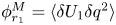 $\phi _{r_1}^M=\langle \delta U_1 \delta q^2 \rangle$, assumes a more significant role. This is expected due to the strong streamwise inhomogeneity of the flow in the transition region. The sign of
 $\phi _{r_1}^M$ is determined by
 $\delta U_1$. In order to facilitate the interpretation of the results, contours of
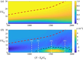
 $U_1$ are shown in figure 9(a). For small
 $r_1$,
 $\delta U_1$ has the same sign as the normal strain rate
 ${\partial U_1}/{\partial x_1}$, thus contours of the latter are also shown in figure 9(b). In the transition region between
 $TR1$ and
 $TR3$, a zone of accelerating flow appears close to the wall, in agreement with the rise of
 $C_f$ shown in figure 1. In the laminar region the flow decelerates, with the strongest negative strain around the centre of the boundary layer.
Contour plots of the mean streamwise velocity  $U_1$ (a) and the normal strain rate
 ${{\rm d}U_1}/{{\rm d}X_1}$ (b). The black dashed curve denotes the
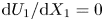 ${{\rm d}U_1}/{{\rm d}X_1}=0$ isoline. The red dashed line indicates the boundary layer thickness.

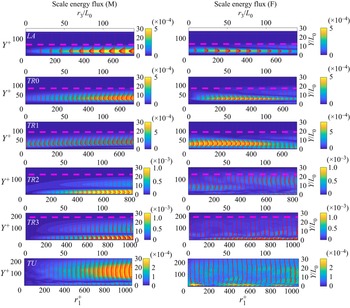
The evolution of the mean (M) and nonlinear interaction (F) components of the energy flux are shown in figure 10. Note the competition between the two components, which is quite subtle. In the laminar region  $LA$,
 $\delta U_1<0$ and the energy flux due to the mean flow leads to forward cascade; however, the nonlinear interaction leads to inverse cascade. The two contributions cancel each other out, and this explains why the total flux shown in the top left-hand panel of figure 8 is very weak for
 $0< r_1/L_0<75$. At
 $TR0$,
 $C_f$ has a minimum and
 $\delta U_1 \approx 0$ for small
 $r_1$, but for larger separations
 $\delta U_1>0$, consistent with the steeper rise of
 $C_f$ at the start of transition. Again at this location the two components compete, with
 $\phi _{r_1}^M<0$ (forward cascade) and
 $\phi _{r_1}^F>0$ (inverse cascade). At
 $TR1$,
 $\delta U_1$ changes sign across the boundary layer (
 $\delta U_1<0$ away from the wall and
 $\delta U_1\ge 0$ close to it; refer to figure 9), but
 $\phi _{r_1}^F>0$ always, leading to overall strong inverse cascade. At
 $TR2$ and
 $TR3$,
 $\delta U_1>0$ close to the wall and very weak further away, while
 $\phi _{r_1}^F$ exhibits a mixture of forward and inverse cascade. Finally at
 $TU$,
 $\delta U_1<0$ away from the wall for large separations (due to the growth of the boundary layer thickness), while again
 $\phi _{r_1}^F$ does not exhibit a clear behaviour. It is evident therefore, that at least in the earlier stages of transition, a strong inverse cascade process exists, which is predominately due to the nonlinear interaction term.
Evolution of the mean (M) and nonlinear interaction (F) components of the energy flux (red vectors) on the  $(r_1, Y)$ plane. The contours are the magnitude of the corresponding flux vector. The spanwise separations are
 $r_3/L_0=8,8,8,8,5,5$ from
 $LA$ to
 $TU$, respectively.

6. Energy fluxes in the $(r_1,r_3)$ plane

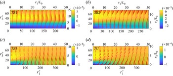
In figure 11 maps of the scale energy flux vectors  $(\boldsymbol {{\phi _r}_1},\boldsymbol {{\phi _r}_3})$ in the
 $(r_1, r_3)$ plane at four streamwise locations are shown; the wall-normal distances correspond to the peak
 $\mathcal {P}_{net}$ of figure 5. Contours of the net energy production are also superimposed. Figure 11(a) confirms the strong inverse cascade at regions of high
 $\mathcal {P}_{net}$, namely
 $5< r_3/L_0<15$. It is clear that the inverse cascade is mainly directed towards the
 $r_1$ direction; in the
 $r_3$ direction it appears only for
 $r_3/L_0>10$, in agreement with figure 5, but it is much weaker. A recirculation pattern in the flow of energy is also evident, i.e. energy emanating from the large net production region flows to large
 $r_1$ and then recirculates back to small
 $r_1$ and
 $r_3$ scales. This recirculation look is much more clear in locations
 $TR2$ and
 $TU$. In
 $TR3$ it is not so evident, possibly because of the narrow range of the
 $r_1$ and
 $r_3$ separations considered.
Scale energy flux vectors  $(\boldsymbol {{\phi _r}_1},\boldsymbol {{\phi _r}_3})$ on
 $(r_1, r_3)$ plane at
 $Y/L_0=5$ for (a)
 $TR1$ and (b)
 $TR2$;
 $Y/L_0=1.3$ for (c)
 $TR3$ and (d)
 $TU$ (red arrows). Contour plots of net production are superimposed. The maximum vector magnitude (corresponding to the longest arrow on each plot) is
 $4.5\times 10^{-4}, 1\times 10^{-3}, 6\times 10^{-4}, 7\times 10^{-4}$ from
 $TR1$ to
 $TU$, respectively.

7. Maps of energy flux in the three-dimensional ($r_1,r_3,Y$) hyper-plane

In the previous sections we examined the evolution of the energy fluxes on the two-dimensional planes  $(r_3,Y), (r_1,Y)$ and
 $(r_1,r_3)$. The most significant finding is that during the transition, a strong inverse cascade of energy exists that originates from the net production peak region and is mainly directed along the
 $r_1$ direction. However, previous results provide only limited understanding because they are visualised on two-dimensional planes, so in this section, we map the energy paths on the three-dimensional hyper-plane (
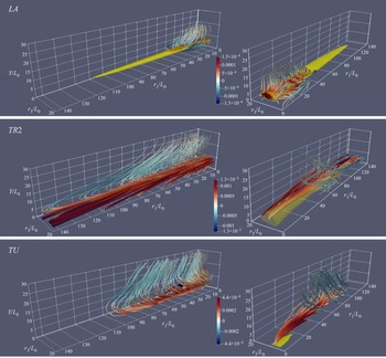
 $r_1,r_3, Y$). These maps are shown in figure 12 for three streamwise locations
 $LA$,
 $TR2$ and
 $TU$, and are visualised from two different viewing angles. To aid understanding, we also superimpose the isosurface
 $0.7\max (\mathcal {P}_{net})$ in yellow colour. For
 $TR2$ and
 $TU$ we focus on different areas of the map; we do this by plotting the stream-tubes crossing small spheres placed at different
 $r_1$ separations (refer to the figure legend for more details).
Maps of energy flux in the three-dimensional ( $r_1,r_3,Y$) hyper-plane in the form of stream-tubes for three streamwise locations. The yellow isosurface denotes
 $0.7\max (\mathcal {P}_{net})$. The stream-tubes are coloured according to the sign of
 $\phi _{r_1}$ (red for positive, blue for negative, thus indicating inverse and forward cascade, respectively). The colour bar refers to the value of
 $\phi _{r_1}$. The radius of the tubes grows with increasing magnitude of the flux vector. Each plot was generated by placing a sphere at a specific location and tracing the stream-tubes crossing the sphere. For
 $LA$, a sphere of radius
 $15L_0$ is placed at
 $(r_1=5L_0, r_3=7.5L_0, Y=5L_0)$ (left and right columns show the same stream-tubes from different angles). For
 $TR2$, a sphere of radius
 $30L_0$ is placed at two points
 $(r_1=20L_0 \mbox { and } 70L_0, r_3=7.5L_0, Y=5L_0)$ (left column) and at
 $(r_1=70L_0, r_3=7.5L_0, Y=5L_0)$ (right column). For
 $TU$, a sphere of radius
 $30L_0$ is placed at two points
 $(r_1=10L_0 \mbox { and } 60L_0, r_3=7.5L_0, Y=1.3L_0)$ (left column) and at
 $(r_1=60L_0, r_3=7.5L_0, Y=1.3L_0)$ (right column).

In the laminar ( $LA$) and transition (
 $TR2$) regions, the net production region (in yellow colour) is centred at
 $r_3=10L_0, Y=5L_0$ and is elongated in the
 $r_1$ direction. At
 $TU$, this region moves closer to the wall (
 $r_3=5L_0, Y=1.3L_0$) and significantly shrinks in the streamwise direction
 $(r_1)$. In all three locations, energy stream-tubes emanate from the production region but their behaviour is different. In the laminar (
 $LA$) region, a weak inverse cascade along the
 $r_1$ direction is observed and then the flow energy pathlines bend upwards to the bulk of the flow and downwards to the wall region. At
 $TR2$, the energy flux is an order of magnitude larger compared with that at
 $LA$. Very strong inverse cascade is present in the
 $r_1$ direction, consistent with figures 8 and 11, but the energy paths then bend back to small
 $r_1$ and
 $r_3$ and towards the bulk of the flow; this explains the recirculating pattern noticed in figure 11. In the turbulent
 $TU$ region, there is still inverse cascade in the
 $r_1$ direction, but it is weaker and confined to a smaller
 $r_1$ domain. Again, once energy has travelled for a sufficient distance in the
 $r_1$ direction, the stream-tubes bend to smaller
 $r_1$ and
 $r_3$ scales and to the bulk of the flow. The flux map at this location is very similar to that of channel flow (Cimarelli et al. Reference Cimarelli, De Angelis and Casciola2013).
8. Analysis of instantaneous interscale energy fluxes in physical space
The analysis presented in the previous sections identified a strong inverse cascade close to the wall, at wall-normal locations  $Y<10L_0$, which is mainly directed in the streamwise direction. In this section, we relate the energy transfer to the physical processes that take place during transition, and in particular to the growth of turbulent spots.
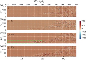
Figure 13 shows four snapshots of the instantaneous wall-normal velocity fluctuation at  $Y=1.3L_0$; the time delay between two snapshots is
 $\Delta t=500$ time units. In figure 13
 $(a)$, two turbulent patches are starting to form at locations
 $(X-X_0)/L_0 \approx 1300$ and
 $1400$. The two patches grow and propagate downstream as shown in figure 13
 $(b)$, and finally merge to form a large turbulent patch, which is clearly visible in figure 13
 $(c)$. This large patch then propagates as a single entity (figure 13
 $d$).
Contour plots of the instantaneous wall-normal velocity fluctuation at  $Y=1.3L_0$ at (a–d) four time instances. The time separation
 $\Delta t$ between two snapshots is 500 time units.

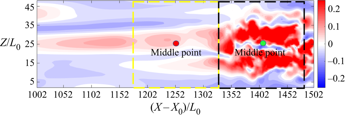
We now focus our attention to the rectangular area marked with a green dashed line in figure 13 $(c)$, which contains both laminar and turbulent regions. This area extends between 1002 and 1502 and between 0 and 50 in the streamwise and spanwise directions, respectively, and covers the region between locations
 $TR1$ and
 $TR2$ (see markings at the bottom of figure 13d). In figure 14 contour plots of the streamwise velocity fluctuations within the selected rectangular area are shown. We choose now two points, one red (at
 $(X-X_0)/L_0=1252$, within a laminar Klebanoff streak) and one green (at
 $(X-X_0)/L_0=1402$, within a streak that breaks down). We think of these two points as fixed middle points around which we consider separations
 $r_1$ up to
 $150L_0$ (consistent with figure 8) and
 $r_3$ up to
 $50L_0$. These separations define two regions,
 $[1177,1327]\times [0,50]$ and
 $[1327,1477]\times [0,50]$, that are marked with dashed yellow and black borders, respectively, in figure 14.
Contour plots of the instantaneous streamwise velocity fluctuations within the rectangular area marked with a green border in figure 13(c).

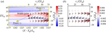
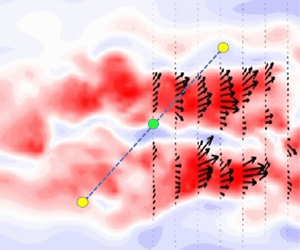
We can investigate the relation between the instantaneous flow and the scale fluxes within these two regions by plotting them in two separate figures. However the interpretation of the results is facilitated if the two figures are superimposed on a single plot. We do this in figure 15(a) for the first region  $[1177,1327]\times [0,50]$. In this panel, we superimpose the interscale energy flux vector
 $(\boldsymbol {{\phi _r}_1}, \boldsymbol {{\phi _r}_3})$ on the
 $(r_1, r_3)$ plane (top and right axes) together with the instantaneous streamwise fluctuations in the
 $(X,Z)$ plane (left and bottom axes). The process is as follows. We select an arbitrary point
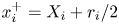 $x_i^{+}=X_i + r_i/2$ to the right of the middle point
 $X_i$, and find the corresponding
 $x_i^{-}=X_i - r_i/2$, as shown in the figure. We then compute the energy flux vector using the fluctuations in these two points, and place the vector at
 $x_i^{+}$ (and since
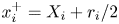 $x_i^+=X_i+r_i/2$, the legends of the top and right axes are
 $r_1/(2L_0)$ and
 $r_3/(2L_0)$, respectively). In this way we can relate directly the instantaneous interscale energy fluxes with the dynamics of the streak breakdown and turbulent patch formation and growth. The right-hand boundary of the area considered in figure 15 is just upstream of the streak breakdown (see also figure 14). Note the stronger streamwise velocity fluctuations when the two high-speed streaks start to break down (at
 $Z/L_0 \approx 10$ and
 $\approx 30$) and the associated inverse cascade. Forward cascade is observed instantaneously around the narrow low-speed streak located in between, at
 $Z/L_0 \approx 20$. In figure 15(b), we present both the flux vectors and contours of the flux component
 $\boldsymbol {{\phi _r}_1}$; the contours show that the inverse cascade is relatively weak at this time instant and location.
Contours of the streamwise velocity fluctuations (a) and of the energy flux component  $\boldsymbol {{\phi _r}_1}$ (b). In both panels, the superposed black arrows indicate the direction of the energy flux vector
 $(\boldsymbol {{\phi _r}_1}, \boldsymbol {{\phi _r}_3})$. The middle point is located at
 $(X-X_0)/L_0=1252$.

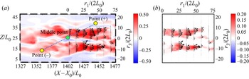
We repeat the process for the region marked by the black border in figure 14. The middle point is now at  $(X-X_0)/L_0=1402$ and is located firmly within the streak breakdown region. Indeed it is surrounded by two high-speed streaks that disintegrate to form a turbulent spot; the spot can be clearly seen in figure 13(c). The results, shown in figure 16, indicate that the large velocity fluctuations inside the streaks contribute to an inverse cascade around the middle point, and this corresponds to the growth of the high-speed streaks within the turbulent spot. Comparison of the streamwise flux components
 $\boldsymbol {{\phi _r}_1}$ (figures 15b and 16b) shows that the inverse cascade is much stronger when the streaks break down. This is because the interscale flux scales with the cube of velocity difference, so a small increase in
 $\delta u_1$ results in much larger fluxes.
Contours of the streamwise velocity fluctuations (a) and of the energy flux component  $\boldsymbol {{\phi _r}_1}$ (b). In both panels, the superposed black arrows indicate the direction of the energy flux vector
 $(\boldsymbol {{\phi _r}_1}, \boldsymbol {{\phi _r}_3})$. The middle point is located at
 $(X-X_0)/L_0=1402$.

In both regions considered, inverse cascade appears when the instantaneous flow accelerates between  $x_i^-$ and
 $x_i^+$. This can also seen in the average picture in figure 8. Note that the interpretation of inverse cascade for fixed values of
 $r_3$ (for example for those values where
 $\mathcal {P}_{net}$ is maximised, as in figure 10) refers to the growth of streaks within spots. This is of course related to the growth of spots themselves, as the latter consist of high-speed streaks that grow individually.
The analysis of the growth of spots as single entities in the spanwise direction using the KHMH formulation is possible, but it is more involved. It would require the identification of a spot using an indicator function as in Marxen & Zaki (Reference Marxen and Zaki2019) and Yao et al. (Reference Yao, Alves-Portela and Papadakis2020), positioning of the midpoint  $X_i$ at the centroid of the spot and integration of the KHMH equation in the scale space around the spot bounding surface. This is a generalisation of the integration over a sphere performed by Hill (Reference Hill2002) and can elucidate very clearly the mechanisms for interscale energy transfer to the spot as a single entity. This is, however, beyond the scope of the present paper.
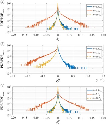
The previous analysis demonstrated that the scale fluxes depend strongly on the distance from the wall and are highly intermittent. This motivates the investigation of their PDF. Figure 17(a) shows the PDFs of  $\boldsymbol {\phi _{r_1}}$ at the streamwise location
 $TR1$ for fixed separation
 $(r_1,r_3)=(50L_0,8L_0)$ and three different wall-normal distances. We also plot the PDFs of the components
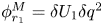 $\phi _{r_1}^M= \delta U_1 \delta q^2$ (figure 17b) and
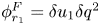 $\phi _{r_1}^F= \delta u_1 \delta q^2$ (figure 17c). In total 55 000 time and spanwise samples were used to construct these PDFs. Although this is not ideal, because spanwise samples smooth out the fluxes around localised spots shown in figure 13, the PDFs still provide a more complete picture compared with time averages.
The PDFs of  $\boldsymbol {\phi _{r_1}}$ (a) with the mean (b) and fluctuating (c) components at
 $TR1$ location for
 $(r_1=50L_0,r_2=0.r_3=8L_0)$.

At the separations considered there is strong inverse cascade, as shown in figure 8. At  $Y=7L_0$, where the inverse cascade is maximised, the shape of the PDF of
 $\boldsymbol {\phi _{r_1}}$ is slightly asymmetric and skewed towards positive values. At the other two locations, the PDF is nearly symmetric resulting in very low time averages. The PDFs of
 $\phi _{r_1}^M$ are one-sided; the sign depends on
 $\delta U_1$ and varies with wall-normal distance. This results in a competition between
 $\phi _{r_1}^F$ and
 $\phi _{r_1}^M$ in the core of the boundary layer. However,
 $\phi _{r_1}^M$ attains small values, and the overall effect on
 $\boldsymbol {\phi _{r_1}}$ is small. Note the presence of rare (low probability) but very strong positive and negative fluxes of
 $\phi _{r_1}^F$ at
 $Y=7L_0$. Similar behaviour has been observed for the PDFs of fluxes in homogeneous isotropic turbulence, see figure 3 in Yasuda & Vassilicos (Reference Yasuda and Vassilicos2018) and also Ishihara, Gotoh & Kaneda (Reference Ishihara, Gotoh and Kaneda2009) and Aoyama et al. (Reference Aoyama, Ishihara, Kaneda, Yokokawa, Itakura and Uno2005), but in this case the time average is negative (standard forward cascade). Therefore the presence of turbulent spots in a transitional flow modifies the average picture, even though the results are spanwise-averaged and the localised spot effect is diluted; this indicates that it must be quite strong. The rare positive and negative events are still there, and it is not clear how the two forms of intermittency, one due to small-scale structures present in turbulent flows and the other due to transition, interact. This motivates a more careful analysis of interscale fluxes, for example one in which the fluxes are conditioned on the flow state (laminar or turbulent) at points
 $x_i^+$ and
 $x_i^-$. Such conditional analysis has been performed by Yao et al. (Reference Yao, Alves-Portela and Papadakis2020) for the second-order structure functions and can be extended to interscale fluxes as well; we leave this for future work.
9. Conclusions
We apply the KHMH equation to analyse the interscale energy flux in a flat-plate boundary layer undergoing bypass transition due to forcing from free-stream turbulence. Energy from the mean flow is injected at a particular spanwise length scale and wall-normal position, both of which are determined by the interaction between the external forcing and the mean shear (linear receptivity process) that takes place in the early development of the boundary layer. This process sets the scene for the subsequent development of the interscale energy transfer and is absent in the fully developed turbulent flows that have been examined so far in the literature. From this production peak, energy fluxes radiate to different directions in physical and scale spaces. Two- and three-dimensional flux maps in the transitional regime show a very strong inverse cascade near the wall (i.e. energy flows from small to large scales) in the streamwise direction. Analysis of the constituent components of the total flux indicates that the inverse cascade is due to the nonlinear interactions between velocity fluctuations. Other components, such as that due to mean flow inhomogeneity, are non-negligible, but are not strong enough to affect the flux direction. As the transition process approaches completion, the maps morph to those encountered in other fully developed turbulent flows, such as channel flow, where there is weak inverse cascade in the streamwise direction, and then the flux vectors bend towards small scales.
Superposition of the instantaneous flux vectors with the corresponding flow fields relates the cascade process to the growth of turbulent structures in the streamwise direction, a unique feature of transitional flows. The sign of the time- and spanwise-average flux is positive across the boundary layer thickness and this is related to predominantly accelerating events that lead to the elongation of vortex structures within a spot, and consequently to the spot itself. These events are absent in fully developed flows. The PDF of the flux is asymmetric and skewed towards positive values. However, strong but rare forward and inverse cascade events are present, as in homogeneous isotropic turbulence.
The present results have painted a picture of interscale transfer in transitional flows that deviates significantly from that of fully developed, wall-bounded, turbulent flows. In the current work, the spanwise averaging dilutes the transfer process within nascent and developing spots, as a large proportion of the flow remains laminar in the early stages of transition. More in-depth investigations using conditional averaging, an operation that naturally accounts for intermittency effects due to transition, are certainly warranted. Such investigations will elucidate the contributions to the average interscale transfer arising from different events, i.e. when the points  $x_i^+$ and
 $x_i^-$ are both located in laminar or turbulent patches, or one is placed in a laminar and the other in a turbulent region. This will allow one to investigate the role of the laminar–turbulent interface in the cascade process.
Funding
H.Y. acknowledges financial support from the Department of Aeronautics, Imperial College London and the Imperial College-CSC scholarship. The authors also wish to acknowledge the UK Turbulence Consortium (UKTC) for providing access to the ARCHER high-performance computing facility through EPSRC grant EP/R029326/1.
Declaration of interests
The authors report no conflict of interest.
Appendix
The budgets for the KHMH equation at two locations,  $TR2$ and
 $TU$, are shown in figures 18 and 19, respectively. Two separation pairs are considered for each location, and all terms are plotted against the wall-normal direction. At small separations, the residual is less than
 $1\,\%$ of maximum production. At large separations, it is less than 4–5 %. Similar results have been found for other streamwise locations and separations.
Budgets of the KHMH equation at location  $TR2$ for
 $(r_3,r_1)=(0L_0,75L_0)$ (a) and
 $(r_3,r_1)=(8L_0,75L_0)$ (b).

Budgets of the KHMH equation at the fully turbulent region ( $TU$) for
 $(r_3,r_1)=(0.1L_0,0L_0)$ (a) and
 $(r_3,r_1)=(18L_0,0L_0)$ (b).