

1. Introduction
The great decline in fertility that took place in most western countries in the late nineteenth and early twentieth centuries, and that has gradually spread over most of the world since then, is one of the major revolutions in human history. Like the Neolithic, industrial and mortality revolutions it has profoundly changed the living conditions of people in large parts of the world. Instead of having six or more children most families today have only two. This development has had a major impact on both macro-economic development and the lives of individuals and families. Lower fertility has contributed in a major way to population ageing, with economy-wide effects on labour supply, consumption patterns, old-age security, and so forth (e.g. Lee Reference Lee2003a, Reference Lee2003b).
There has been considerable debate in the literature on how this change came about in the western world in the nineteenth and early twentieth centuries. Some have argued that even though it might be tempting to connect fertility decline to other major changes occurring at about the same time, such as mortality decline, industrialisation and urbanisation, fertility decline was mainly caused by attitudinal change related to the spread of new ideas about family limitation as well as increased knowledge of contraception, rather than the economic changes as such. This view found quite strong support in the European Fertility Project carried out at Princeton University in the 1960s and 1970s (Coale and Watkins Reference Coale and Watkins1986; Lesthaeghe Reference Lesthaeghe1977; Knodel Reference Knodel1977; Knodel and van de Walle Reference Knodel and van de Walle1979; see also Cleland and Wilson Reference Cleland and Wilson1987; Woods Reference Woods2000, chapter 4).
Other scholars have questioned this strong focus on innovation aspects and cultural, or religious, explanations in the conclusions of the European Fertility Project, as well as its rejection of socioeconomic variables as the triggering mechanisms. Several studies using more detailed demographic and socioeconomic data, as well as more advanced statistical methods, have found these kinds of demand-oriented variables to have played an important role in fertility decline (e.g. Richards Reference Richards1977; Mosk Reference Mosk1983; Schultz Reference Schultz1985; Crafts Reference Crafts1984; Galloway, Hammel and Lee Reference Galloway, Hammel and Lee1994; Galloway, Lee and Hammel Reference Galloway, Lee and Hammel1998a; Brown and Guinnane Reference Brown and Guinnane2002; see also Brown and Guinnane Reference Brown and Guinnane2007).
Related to this debate is also the question whether childbearing before fertility decline was deliberately controlled or not. Scholars emphasising innovation aspects and attitudinal change have also been inclined to argue that fertility in pre-transitional Europe was not deliberately controlled but ‘natural’.Footnote 1 Ansley Coale, the leader of the European Fertility Project, argued that fertility was probably not within the ‘calculus of conscious choice’ before the fertility decline, and hence the main explanation behind the fertility transition was the innovation of families starting to adjust fertility within marriage to economic circumstances (Coale Reference Coale1973, p. 65; Coale and Watkins Reference Coale and Watkins1986). As a consequence, females stopped childbearing after having reached a certain target family size; in other words, the control was parity-specific.
Other scholars have, however, questioned these conclusions, emphasising that families in pre-transitional Europe also controlled their fertility deliberately, even though it was often done in a non-parity-specific way (see, e.g., Bean, Mineau and Anderton Reference Bean, Mineau and Anderton1990; David and Sanderson Reference David, Sanderson, Engerman and Gallman1986; David and Mroz Reference David and Mroz1989; Szreter Reference Szreter1996; Bengtsson and Dribe Reference Bengtsson and Dribe2006; Van Bavel Reference Van Bavel2004; Van Bavel and Kok Reference Van Bavel and Kok2004). Consequently, the explanations behind the great decline in fertility have also changed. Scholars emphasising the existence of deliberate non-parity-specific control before the transition are also inclined to stress these factors as important in the decline itself, rather than simply focusing on the invention of parity-specific control (Crafts Reference Crafts1989; Szreter Reference Szreter1996).
The aim of this article is to study the importance of socioeconomic and demographic factors in the secular decline of fertility in Sweden using county-level demographic and socioeconomic data. The development of total and age-specific marital fertility is analysed and related to broader socioeconomic changes, for example mortality decline, industrialisation and urbanisation, using panel regression analysis. The results are in line with expectations from standard economic-demographic models in which the notions of demand and supply of children are used to link fertility to mortality, education, income, urbanisation and female earning potentials. The study clearly connects to the recent studies on different parts of Germany, which, by using a similar methodology, have found these kinds of variables to have been of crucial importance in the decline of fertility (Galloway, Hammel and Lee Reference Galloway, Hammel and Lee1994; Galloway, Lee and Hammel Reference Galloway, Lee and Hammel1998a; Brown and Guinnane Reference Brown and Guinnane2002).
2. The Swedish case
Despite the comparative abundance of historical demographic data in Sweden there is no massive literature on the Swedish fertility transition. Even though there have been a couple of individual studies of the various aspects of the fertility transition in Sweden, we still lack a comprehensive analysis of this important process that takes into account both the demographic development and its socioeconomic context, and tries to explain the changes taking place. There is no study using panel regression models and disaggregated data for the whole period of the fertility decline with the aim to assess the impact of changes in vital socioeconomic and demographic variables on the development of fertility. What follows is a brief review of the most notable studies dealing with Swedish fertility development in the period of the fertility transition.Footnote 2
The basic demographic patterns of the fertility decline in Sweden have been known for a long time, and were, for instance, outlined by Hofsten and Lundström (Reference Hofsten and Lundström1976) in their demographic history of Sweden.Footnote 3 Besides presenting the sources of historical demographic data they also present the basic demographic indices at the national and regional levels. Due to differences in the methods of calculation their figures differ slightly from what is presented here (see the data section below). While giving very useful descriptions of the demographic development, they do not offer much in terms of explanations and do not really relate the demographic picture to the socioeconomic changes taking place. There have been a few studies trying to do just that. In a seminal article Carlsson (Reference Carlsson1966) discussed the causes of fertility decline, making what soon became a classic distinction between ‘innovation’ and ‘adjustment’ as explanations behind fertility transitions more generally. In the specific Swedish case, analysing geographical patterns of fertility, he argued that since the diffusion of birth control after 1880 did not follow a geographic pattern, with the possible exception of the northern parts of the country, the decline in marital fertility was explained by some kind of adjustment process and not by a spread of new knowledge or technology in birth control.
Wilkinson (Reference Wilkinson1973) made an early attempt to analyse the Swedish fertility decline using multivariate regression models. Looking at the aggregate national development he found clear structural shifts in the determinants of fertility. Controlling for infant mortality, cost of children and emigration, a proxy for husband's wage had a positive effect on the crude birth rate during the whole period from 1870 to 1965, while a proxy for wife's potential earnings had a negative effect on the birth rate after about 1910, when the decline was already well under way.
The most thorough economic historical analysis of the Swedish fertility transition is the one by Mosk (Reference Mosk1983), who compared Sweden with Japan in trying to establish a link between structural change in demographic behaviour (nuptiality and fertility) and the declining importance of ‘patriarchy’. The main hypothesis is that as the traditional stem-family system became weaker, parental control over children's decision to marry and form a family diminished, which led to lower ages at marriage and controlled fertility because demand for children declined when couples could decide for themselves without the influence of the older generation. Mosk analysed both the national pattern and county-level data, using more descriptive methods and multivariate regression analysis. Regarding the latter, however, only the final part of the transition was analysed using disaggregated data. The results were generally supportive of demand-oriented explanations. Infant mortality had a positive effect on marital fertility (measured by the index Ig), while a proxy for education (proportion of schoolchildren in 1920) had a negative effect. Neither male wages nor the proportion employed in industry yielded statistically significant effects, and female wages affected marital fertility in the expected negative way in 1920, but not before that time. Even though Mosk's analysis contributed a great deal to the knowledge of the Swedish fertility transition, there are some aspects that deserve more attention. The disaggregated data were not analysed multivariately for the entire period of the transition, due to a lack of explanatory variables. In the present study, new data on the socioeconomic context of the counties will be used in a panel analysis of the regional changes in fertility during the entire period from 1880 to 1930, and will thus serve to considerably extend the analysis made by Mosk. In addition, age-specific marital fertility will be analysed rather than the Princeton index of total marital fertility (Ig).
Schultz (Reference Schultz1985) has made the greatest use so far of the regional economic and demographic data in a study using county data on total and age-specific fertility, and a set of economic explanatory variables at the county level. His main focus was to study the exogenous influence of women's wages on fertility using instrumental variable estimations, where the relative price of animal products (mainly butter) was seen as the main determinant of female relative wages. Controlling for child mortality (0–10), proportion urban, and employment in textile and food industries, the results confirmed an important exogenous role of higher female relative wages for lower fertility, both total and marital.
The studies trying to explain the fertility transition in Sweden have been quite favourable to theories linking fertility decline to the lower child mortality and economic modernisation that characterised the period. This stands in contrast to the great scepticism towards these kinds of explanations coming out of the European Fertility Project, where most emphasis, as has already been mentioned, was put on innovation aspects in the diffusion of new attitudes towards deliberate birth control. However, in a study dealing only with central Sweden before and in the early phases of the decline (1855–90) Lockridge (Reference Lockridge1984) identified areas in which fertility seems to have been controlled early on (measured by the Coale-Trussel index m). Since he failed to find any socioeconomic differences between the geographical units analysed, he conjectured that this early adoption of deliberate control was culturally determined in some way. He also found some support for this conclusion from literary sources on the strength of the church in the different areas, but admitted that the conclusions in this regard were very tenuous (see also Larsson Reference Larsson1984). He did not, however, present much data on socioeconomic conditions in the different areas, neither did he make a multivariate analysis. Thus, it is difficult to draw firm conclusions from this analysis regarding the explanations behind the regional differences in central Sweden in the degree of parity-specific control. It is also unclear how the early adoption of parity-specific control in this area would be related to the general decline of fertility in Sweden as a whole.
It is quite clear that the fertility decline in Sweden coincided with industrialisation and increasing urbanisation, but the decline of fertility was completed in a country still dominated by agriculture, and where more than two-thirds of the population lived in rural areas. Already in the first half of the nineteenth century production of textiles had grown rapidly as a result of increased domestic demand, following increased agricultural productivity and higher incomes for farmers (Schön Reference Schön2000, chapter 2). This created an early, domestically oriented, industrialisation in Sweden and was an important preface to the real breakthrough of industrialisation and modern economic growth in the second half, and especially the last quarter, of the nineteenth century. While GDP per capita grew by about 0.5 per cent annually in the decades before 1850, the annual average growth rate between 1850 and 1890 was 1.9 per cent (Schön Reference Schön2000, p. 139). For about 60 years, from 1890 to 1950, Sweden had among the highest rates of economic growth in the world and was definitely being transformed from an agrarian society into a modern industrial nation, although this process was by no means finished in 1930 when the fertility transition was completed. The proportion of the population living in towns, for example, increased from 19 per cent in 1890 to 32 per cent in 1930, and in the same period the proportion of the labour force employed in industry increased from 17 to 26 per cent, while the proportion employed in agriculture declined from 58 to 34 per cent (Statistics Sweden 1999, p. 42; Schön Reference Schön2000, p. 233). From 1900 to 1930 the proportion of women over 15 employed outside the home (excluding women on family farms) also increased from 19 per cent to 27 per cent (Stanfors Reference Stanfors2007, p. 74).
In the nineteenth and early twentieth centuries Sweden was culturally comparatively homogenous. A very large majority of the population had Swedish as their mother tongue, belonged to the state Lutheran church and was born in the country. Less than one per cent of the population in 1900 was born abroad and only 0.3 per cent were non-Swedish nationals (BiSOS A 1900; see data appendix). The only minority groups of any importance were Sami people and Finns, who, in Norrbotten county, where they were most prevalent, constituted about 3 per cent and 16 per cent of the population respectively. At the national level, however, they made up only fractions of a per cent. Thus, there were no major differences in terms of religion, language or ethnicity in the country. Naturally, some differences existed in religious orientation and strength of the church (Larsson Reference Larsson1984), but nothing compared to the religious and language barriers in some other parts of Europe. This makes Sweden an almost ideal setting when studying the interplay between socioeconomic change, mortality decline and fertility.
In sum, previous studies on the Swedish fertility transition provide quite a good picture of the demographic development, while there is considerably less in terms of explanatory analyses using disaggregated data. Strictly speaking, it is only the study by Schultz that analyses county-level data for the entire period of transition using multivariate regression models and data on socioeconomic and demographic variables. The present study adds to his work by using fixed-effects panel regression models and new data on education, regional wages and migration, as well as on voting behaviour for part of the transition. This enables an analysis of the socioeconomic and demographic determinants of the decline in fertility in a setting characterised by comparatively small regional differences in religion and religiousness, ethnicity and language. The study connects to more recent studies on Germany which have applied similar methods and showed the importance of socioeconomic and demographic variables in explaining the fertility transition in contrast with widely held views on the primacy of innovation aspects in the fertility decline (Galloway, Hammel and Lee Reference Galloway, Hammel and Lee1994; Galloway, Lee and Hammel Reference Galloway, Lee and Hammel1998a; Brown and Guinnane Reference Brown and Guinnane2002).
3. Data and measures
The demographic data come from the Swedish official population statistics at national and county level. From 1749 to 1860 the data were organised in the so called Tabular Commission (Tabellverket), which published yearly tables of vital events and tables on population by age and sex, as well as occupational distribution every five, or sometimes every three years. From 1860 onwards the newly established Bureau of Statistics, or Statistics Sweden, reorganised the production of demographic data. Now there was a census every ten years which provided a quite detailed account of the population in different subgroups and geographical areas, and in addition vital events were published yearly (see Hofsten and Lundström Reference Hofsten and Lundström1976; see also data appendix).
Thus, yearly information is available on most demographic events of interest, while the population at risk is only available every five or, after 1860, every ten years. At national level Sundbärg (Reference Sundbärg1907) adjusted the older, and less reliable, statistics and also estimated the annual population by age and sex, and by marital status, from the census figures. Although his revisions have become the ‘official’ statistics published by Statistics Sweden, these annual population data by age, sex and marital status are based on quite approximate calculations and the exact method is not always explicit (Hofsten and Lundström Reference Hofsten and Lundström1976, p. 29; Lundh Reference Lundh2003).
This implies that age-specific fertility as well as age-specific marital fertility, and thus the corresponding summary measures of total fertility (TFR) and total marital fertility (TMFR), can be calculated for Sweden as a whole back to the mid eighteenth century. At county level, however, we are not equally fortunate. Although there are yearly data on number of births by age of mother at county level back to 1774, the population at risk is available only in the census years. Moreover, before 1881 births by age of mother were not separated according to legitimacy. For these reasons the regional pattern of marital fertility will be analysed using data around the censuses from 1880 to 1930, which is the period of secular fertility decline in Sweden. It should be pointed out that Sweden is one of very few countries for which age-specific marital fertility rates at regional level can be calculated in this period, which allows us to study the impact of socioeconomic variables not only on composite indexes such as the Ig or the General Marital Fertility Rate (number of legitimate birth per 1000 married females aged 15–49), but on the age-specific marital rates.
In the descriptive analysis below the age-specific and total marital fertility rates are calculated using live legitimate births by age of mother in the year before and after the census.Footnote 4 Since the census refers to 31 December the census population constitutes a mid population for the vital events in the census year and the year after. In the multivariate regression analysis fertility is instead calculated as the number of live legitimate births by age of mother in the year following the census to the risk population in the census. The difference is not large, but in an explanatory model it is more appealing to think in terms of risk, and since all explanatory variables refer to the census year there will not be any problem of simultaneity in the analysis.
4. Fertility decline in Sweden: national and regional patterns
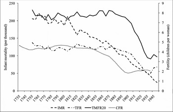
Before turning to a more detailed analysis of the fertility development at county level, a picture will be given of the development at national level. Figure 1 displays the infant mortality rate (IMR), period of total fertility (TFR) and total marital fertility for women over 20 (TMFR20) in Sweden as a whole from the mid eighteenth century to the mid twentieth century as five-year averages, as well as accumulated fertility at age 50 by birth cohort (CFR). Despite some medium-term fluctuations the long-term level of fertility was quite stable until the last quarter of the nineteenth century; between four and five children per woman, or around eight children for married women. Beginning around 1880, period fertility started to decline steadily until the beginning of the 1930s when it started to increase again. Between 1880 and 1900 the decline was modest, but gained considerable speed thereafter. This period – between 1880 and 1930 – marks the decline of Swedish fertility. It constitutes an important phase of the demographic transition, about 100 years after infant mortality started its continuous decline. Looking at the cohort fertility pattern, the decline starts from the cohorts born around 1850, in other words, women who were at prime childbearing ages in the early 1880s when period fertility started to decline.
Period and cohort fertility and infant mortality in Sweden, 1735–1950
Source: Statistics Sweden 1999, tables 3.3, 3.4, 3.7 and 5.1.
Note: IMR: infant mortality rate (per thousand). TFR: period total fertility rate. TMFR20: period total marital fertility rate in ages over 20. CFR: accumulated cohort fertility rate at age 50.
Labels on the x-axis refer to the ending year in quinquennial rates for IMR, TFR and TMFR20 (1751-5, 1756-60, etc.) and year of birth for CFR.

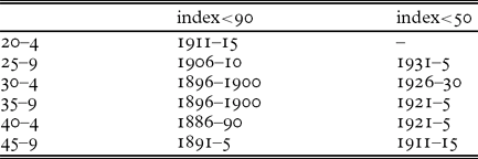
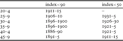
Marital fertility follows closely total fertility, showing that the decline can mainly be attributed to a decline in marital fertility rather than changes in nuptiality, which is also a well-established conclusion from previous research on the European fertility transition (Carlsson Reference Carlsson1966; Coale and Watkins Reference Coale and Watkins1986). For this reason the analysis in the rest of the article is limited to marital fertility. Turning to the age-specific pattern of marital fertility, Table 1 shows the quinquennia when an index of age-specific marital fertility (1871/75 = 100) had fallen to 90 and 50 per cent, which correspond, respectively, to a 10 and 50 percentage point decline compared to the 1871/75 level. Marital fertility had dropped by 10 percentage points by 1896/1900 in all age groups over 30, but not until 1911/15 in the youngest age group.
Period when index of age-specific marital fertility fell below 90 and 50 of its 1870/1 level
Source: Statistics Sweden 1999, table 3.4.
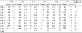
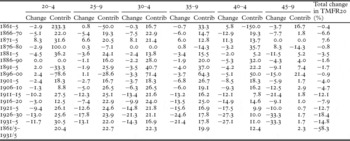
If we instead look at the percentage change in marital fertility between quinquennia (Table 2), it is clear that the older age groups show a stronger decline early in the transition, even though all age groups over 25 show a continuous decline after about 1880. Over time the decline gets progressively stronger in younger age groups. In Table 2 the percentage contribution to change in total marital fertility (TMFR20) in different age groups is also displayed. Clearly, the development in the younger age groups – the prime childbearing ages – contributes more to the overall decline than does the development in the older age groups. Over the whole period the age groups 20–24 to 35–39 contribute about 20 per cent each to the decline, while the contributions of the two higher age groups are about 12 and 2 per cent respectively.
Change (%) in age-specific marital fertility in Sweden since previous quinquennium and contribution (%) to quinquennial change in TMFR20 in different age groups
Source: Statistics Sweden 1999, table 3.3.
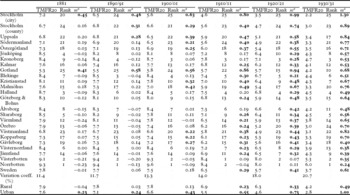
We now turn to a more disaggregated analysis of the fertility transition in Sweden by looking at the development at county level. At the time dealt with here Sweden was divided into 24 counties plus the capital city of Stockholm, which is separated from Stockholm county in the official statistics. Table 3 shows that marital fertility varied between 5.3 and 9.3 in 1881 and 2.2 and 6.0 in 1930/31, in other words by around four children per woman at both ends of the transition. The coefficients of variation show that county differences actually widened, in relative terms, during the transition. Table 3 also reports the ranking of counties from high to low marital fertility, and shows a relative stability in the county ranking over time.
Indicators of marital fertility in Swedish counties, 1881–1930/1

Source: See data appendix.
Note: a Bold figures indicate m > 0.20.
Ever since Louis Henry's introduction of the concept of natural fertility there has been a strong tendency in the literature to equate deliberate fertility control with parity-specific control; in other words, childbearing stops after reaching a certain target number of children (Henry Reference Henry1961; Coale and Watkins Reference Coale and Watkins1986). One way of measuring the degree of parity-specific control is by the m index, which is a measure of the deviation from natural fertility in the age-specific pattern (Coale and Trussell Reference Coale and Trussell1974, Reference Coale and Trussell1978). Values of m above 0.2 are usually taken as a large enough deviation from natural fertility to indicate that fertility was controlled in a parity-specific way. Although there have been numerous criticisms against this way of modelling natural fertility, and although several alternative formulations and estimation techniques have been proposed and presented, it has survived to become widespread, probably because of its simplicity and hence its value for comparisons (see, e.g., Page Reference Page1977; Broström Reference Broström1985; Wilson, Oeppen and Pardoe Reference Wilson, Oeppen and Pardoe1988). Mainly for reasons of comparison the standard formulation devised by Coale and Trussell has been used, by which m is estimated by ordinary least squares regression.
Table 3 reports the m-values for the Swedish counties and all values of m above 0.2 are marked in bold. Gotland and the city of Stockholm show signs of parity-specific control already in 1881, which also fits well with the low levels of marital (and total) fertility in these counties. It also offers some support for the claims made that the inhabitants of Gotland practised deliberate control very early on; well before the beginning of the secular decline in fertility (Wohlin Reference Wohlin1915). Then follow the counties of southern and middle Sweden, and lastly the northernmost counties. In the final period all counties show values of m above 0.2, indicating widespread adoption of parity-specific control.
5. Determinants of fertility decline
Following the framework outlined by Easterlin and Crimmins in their book The Fertility Revolution (Reference Easterlin and Crimmins1985), the number of children born in a family can be seen as determined by three separate sets of factors: the demand for children, the supply of children and the cost of fertility regulation. Even though this framework does not fully explain all aspects, it captures many of the important factors determining the great decline in fertility.Footnote 5
The demand for children is defined as the number of children a couple would want if there were no costs to limit fertility. It depends on family income and the costs of children in relation to other goods. Children are assumed to be normal goods, implying that a higher income increases fertility, while a higher relative price of children lowers fertility. The demand for children is also dependent on the preferences for consuming other goods, and a higher demand for consumption of other goods lowers the demand for children. In addition, the demand for child quality is often believed to have increased as a result of economic changes following industrialisation and urbanisation, through which education and other investments in children have become ever more important (Becker Reference Becker1991). Thus, demand for child quality has increased at the expense of child quantity, which helps to explain why fertility does not increase together with rising incomes in the process of modern economic growth.
The supply of children is defined as the number of surviving children a couple would get if they made no conscious efforts to limit the size of the family. Thus, it reflects natural fertility as well as child survival. High child mortality constitutes a limit on this potential supply and cultural factors outside the immediate control of the family, such as breastfeeding practices, which influence the level of natural fertility, might also impose such a limit.
Finally, the costs of fertility regulation can be defined as the direct monetary costs as well as psychic costs of regulating fertility. New, more positive, attitudes towards fertility control among broader segments of the population will act to lower these costs. In a similar way easy access to modern contraceptive methods will affect these costs.
In this way fertility decline is seen as a result of both adjustment of behaviour to new socioeconomic circumstances and innovation in the form of new attitudes and methods lowering the costs of fertility control (cf. Carlsson Reference Carlsson1966). Nonetheless, it is quite clear that Easterlin and Crimmins themselves put most emphasis on the changing demand for children following modernisation of society, and a lower supply of children mainly as a result of declining infant and child mortality. In what follows, this simple framework will be employed in analysing marital fertility in Swedish counties.
The dependent variable is a measure of total marital fertility for women aged 20–49, where the underlying age-specific fertility is calculated as the number of live legitimate births to women in the age group in the year following the census in relation to the number of women in that age group on 31 December the preceding year. Thus, instead of being a rate in its true meaning, this measure is better thought of as the risk of having a birth conditioned upon being alive and married at the beginning of the year. All explanatory variables refer to the census year, in other words the year before the recorded births (see data appendix for sources). Regression models are also estimated using age-specific marital fertility as dependent variables, in order to see the impact of the explanatory variables in different ages.
The supply of children is measured by the mortality rate in ages 0–4.Footnote 6 A clear relationship between infant or child mortality and fertility has also been found in some historical studies of fertility (Galloway, Lee and Hammel Reference Galloway, Lee, Hammel, Montgomery and Cohen1998b; Reher Reference Reher1999), although the European Fertility Project concluded that infant mortality decline was not a main cause of fertility decline in Europe (van de Walle Reference Van de Walle, Coale and Watkins1986), and a similar result was found in a study on Bavaria (Brown and Guinnane Reference Brown and Guinnane2002). The fact that the decline in infant mortality in Sweden started about 100 years before the beginning of fertility decline does not immediately imply that there can be no relation between the two. As discussed by Easterlin and Crimmins in outlining their model, a long delay may simply result from a too low supply of children to begin with, and, if the demand for children does not decrease, fertility will not either since the demand will still exceed the supply. Not until the demand for children is approximately equal to actual fertility will lower child mortality (higher supply of children) depress fertility.Footnote 7
The demand for children is a function of a multitude of factors: household income, value of parental, primarily the mother's, time, as well as other costs and benefits of children. The availability of data in most historical settings, however, puts quite strong limits on what can actually be done in terms of empirical analysis. In many cases we have to lean on rather rough proxies, which has also been a more general problem in much research on the European fertility transition.
Education is a central variable in this context. It may contribute to lower benefits of children due to less labour input when children are at school. Although basic education came without a charge in Sweden, there were most likely costs related to school material that, at least in the long term, could make a difference. The biggest contribution of education to the costs of children in the long run, however, must have been to provide for a large number of children who were not able to start working properly until they finished school. The differences in educational orientation between the counties is measured by the number of teachers in basic education (folkskola, småskola) per 100 children aged 7–14, which was the school age defined by the authorities (see Statistics Sweden 1974, p. 20). Higher teacher intensity is supposed to reflect a greater importance of education, which, in turn, should have a depressing effect on fertility through higher costs, and lower benefits, of children.
Industrialisation is often viewed as an important factor affecting the demand for children, because children are viewed to be of greatest use to their families in a more traditional agrarian setting where they can help out at an early age. When industrial employment becomes increasingly important, getting a formal job in a factory becomes crucial. The gradual decline of child labour quite early on in the industrialisation process made it more difficult to actually employ children, and therefore the direct benefits of children declined (Olsson Reference Olsson1980; see also Cunningham and Viazzo Reference Cunningham and Viazzo1996). In addition, working in a factory was more difficult to combine with looking after small children compared to working on a farm, where work and childminding could be combined, or older children could look after the younger ones. Thus, higher industrial employment can be expected to be related to lower fertility. This variable is measured by the number of male industrial workers in relation to the male population aged 15–64, and calculated from data on occupational structure.
A related factor is the degree of urbanisation. For similar reasons to those discussed above, living in a town can be expected to have implied greater difficulties in looking after small children compared to living on a farm. In addition, cramped housing probably added to these difficulties. Hence, a higher proportion of the population living in towns is expected to be related to lower fertility, due to a lower demand for children.Footnote 8
In modern societies one of the biggest costs of having children is the value of parental time invested in children, which can be approximated by the income lost while giving birth and rearing children. Since childbearing is always a female task, and in most pre-1960s contexts childrearing is as well, women's earnings, or earning potentials, are usually used as a proxy for the value of parental time (Mincer Reference Mincer and Christ1963). Controlling for male wages, female relative wages proxy the earning potential of women in the labour market, and thus serve as a measure of the opportunity cost of children. Since it is very difficult to get good data on sex-specific wages at county level for Sweden, rather crude approximations had to be made. Female relative wages are measured as the ratio between female and male summer day wages in agriculture, except for Stockholm city where wages of unskilled workers were used instead. It would, of course, have been preferable to use more data on industrial wages in this kind of measure. The problem, however, is that they are very difficult to obtain. In a recently published book on regional wages in Sweden, industrial wages are only given for groups of counties but not for individual ones (Lundh et al. Reference Lundh2004).
The real wages for men are used as a proxy for family income, which serves to measure any potential income effect on fertility. Thus, higher real wages should increase fertility if such an income effect were important. For Stockholm county, wages of unskilled labourers were used, while for all other counties day wages in agriculture were used instead, for reasons already explained. The nominal wages were deflated by the prices of a food basket (see data appendix).
Migration may affect marital fertility in different ways. Migration is an important indicator of the economic development in a region. High out-migration testifies that economic opportunities in terms of average living standards, or employment opportunities, are comparatively unfavourable, while in-migration to a region is a prime sign of economic dynamism. To the extent that fertility is sensitive to economic conditions, regions with high out-migration might have relatively low fertility. At the same time large flows of migrants from regions facing economic difficulties might have positively affected the labour market conditions for those who stayed behind, thereby facilitating family formation. These kinds of effects have proven important in cases where living standards have been very low and migration rates high, such as in Ireland after the famine in the 1840s (Ó Gráda and O'Rourke Reference Ó Gráda and O'Rourke1997). Finally, it is possible that migration could be a contributing factor in diffusion of knowledge in a society with a less developed information technology. In-migration to a region might then have the effect of bringing in new ideas and attitudes about birth control and the proper size of a family, which in turn might have affected marital fertility in the region through a lower cost of regulation. A measure of accumulated net migration (in-migration minus out-migration per 1,000 population in the previous ten-year period) is included to control for these potential effects of migration.
In a context where fertility declines before the introduction of modern contraceptives, attitudes towards deliberate birth control might have affected the costs of fertility regulation. To the extent that these kinds of attitudes differed between counties, they depended on a complex set of factors. Better flows of information might have promoted the spread of new ideas. Differences in the degree of secularisation and voting behaviour, for example the proportion people voting for social democrats, liberals or other parties with modernist ideologies, have been used as indicators of the degree to which these new ideas permeated different communities (e.g. Lesthaeghe Reference Lesthaeghe1977; Teitelbaum Reference Teitelbaum1984, chapter 7; Galloway, Hammel and Lee Reference Galloway, Hammel and Lee1994; Brown and Guinnane Reference Brown and Guinnane2002; see also Derosas and van Poppel Reference Derosas and van Poppel2006). In Sweden, suffrage did not become universal for men until the general election of 1911, and for women not until 1921. Before this time, according to the election statistics, only about 20–30 per cent of the adult male population was entitled to vote (see data appendix). Moreover, the modern party system with social democrats, liberals and conservatives was not established before the beginning of the twentieth century. Taken together, this makes it very difficult to use voting data before 1910, when the fertility transition was already well under way. In the empirical analysis the impact of differences in the proportion voting for the socialist parties (the Social Democratic Party and, after 1917, the Communist Party) on differences in the level of marital fertility between the counties will be analysed for the period 1910–30.
6. Empirical results
The data are structured as a panel of 25 county observations for six census years. Two different models are estimated, both including categorical time variables that capture nation-wide changes between the censuses: a pooled ordinary least squares regression (OLS) measuring level differences between counties, and a fixed-effects panel regression model (FE), measuring the impact of changes over time in the explanatory variables on fertility taking unmeasured county-level heterogeneity into account. The fixed-effects model can be written as:

where v i is the county-specific residual and ϵit is the ‘individual’ residual.Footnote 9 The fixed-effects specification implies that the group-specific heterogeneity is assumed to be constant over time, and thus controls for time-invariant differences between groups (counties in this case) that are not captured in the model. Thus the FE estimations essentially model changes within units between panels rather than level differences between units as in the pooled OLS model. Differences between units that do not change over time are captured by the unit-specific error term (the fixed effects).
One problem often plaguing these kinds of models is endogeneity in the explanatory variables. For example, lower fertility, and thus fewer children, may increase parental investment in each child, which in turn may increase the survival chances of these children and thus lower child mortality. There are other conditions, such as breastfeeding habits, health or nutritional factors that may affect both fertility and infant and child mortality at the same time, which make it difficult to view child mortality as a completely exogenous variable. Some have tried to deal with this problem using instrumental variable (IV) estimations. The problem, however, is to find a suitable instrument that picks up the exogenous part of the variation in the variables, and using bad instruments biases the estimations (e.g. Wooldridge Reference Wooldridge2006, p. 519). In the case of child mortality, various instruments have been tried: male adult mortality, elevation above sea level and population density (Galloway, Lee and Hammel Reference Galloway, Lee, Hammel, Montgomery and Cohen1998b; Brown and Guinnane Reference Brown and Guinnane2002). Given the comparatively large units of analysis and the geographical context of Sweden, neither elevation above sea level nor population density was judged proper in this case. Data on male adult mortality are readily available and were considered as an instrument for exogenous variation in child mortality, following the work of Galloway, Lee and Hammel (Reference Galloway, Lee, Hammel, Montgomery and Cohen1998b), but were not valid in the Swedish case. A good instrument should be uncorrelated with the dependent variable but correlated with the endogenous variable, in this case child mortality. Simple linear regression shows that mortality for married men is indeed correlated with child mortality (coefficient = 2.52, p-value = 0.000, correlation coefficient = 0.58), but, somewhat surprisingly, it is also statistically significantly correlated with marital fertility (coefficient = 3.59, p-value = 0.000, correlation coefficient = 0.72), which makes it unsuitable as an instrument. Because no other valid instruments are available, the estimated effects of child mortality on fertility need to be interpreted with caution when it comes to causality.
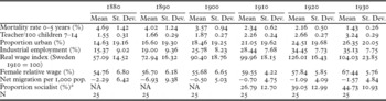
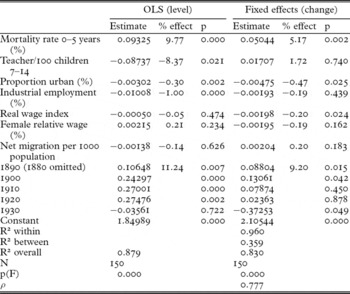
Table 4 displays the means and standard deviations of the variables in the panel, and Table 5 shows estimations of the pooled OLS and FE models. It also provides the percentage change in total marital fertility of a one unit change in the explanatory variables. In the FE model the within-county R2 is 0.96, which implies that the model accounts for 96 per cent of the variation within counties over time, while the between-county R2 is only 0.36.
Descriptive statistics of variables in regression

Note:
a. 1910 refers to the parliamentary elections of 1911; 1920 is an average of the parliamentary elections of 1920 and 1921; and 1930 is an average of the elections of 1928 and 1932. The 1921 election was the first with universal suffrage for both men and women.
Source: See data appendix.
OLS and fixed-effects panel regression estimates of total marital fertility

Note: The dependent variable is the natural logarithm of total marital fertility 20–49 years. P-values are based on (White/Huber) heteroskedasticity robust standard errors.
% effect in y of a one unit change in X is given by 100*(exp(b)-1)).
Source: See data appendix.
The effect of child mortality is, as could be expected, positive and statistically significant in both estimations. Although this finding is consistent with the idea that declining child mortality increases the supply of children, which gives incentives to families to limit fertility, the potential endogeneity problem prevents a firm conclusion regarding the direction of causality.
The variable measuring educational orientation negatively affects fertility in the level regressions, which is also what could be expected. One more teacher for 100 children aged 7–14 is associated with about 8 per cent lower marital fertility in a county. Since this variable reflects more general differences in educational orientation between the counties, it should serve as a valid indicator of the importance of child quality, which led parents to reduce the quantity in order to be able to invest more in each child's quality. In a study of fertility decline in the United States, Wahl (Reference Wahl, Goldin and Rockoff1992) also concluded that changing prices of child quantity and quality were the most important explanations for the transitions to low fertility, and that the expansion of education, together with increased child survival and incompatibility between work and family were crucial factors in this change. However, the absence of a corresponding effect in the FE estimations indicates that changes in this variable are not important in explaining changes in fertility within counties over time, although it seems important behind level differences in marital fertility between counties.
The proportion of the population living in towns is associated with lower fertility in both the OLS and FE estimations. A one-percentage point higher urbanisation lowers marital fertility by 0.3 and 0.5 per cent respectively. This is also consistent with the expectation that the urban way of living is less compatible with childbearing and childrearing. In the rural context women's work usually took place on the farm and in the household, which facilitated a combination of work and childcare. Moreover, children had more tasks to perform in the rural economy compared to the urban industrial one, which further lowered the benefits of children. In many cases living conditions were also more overcrowded in urban areas, which put even more restrictions on large families. There is also an additional negative effect of higher industrial employment in the OLS model, and, although not statistically significant, also in the FE model.
Increasing male real wages seem to be associated with declining marital fertility (FE model), while there is no corresponding effect of inter-county differences in real wages on fertility (OLS model). Increasing real wages reflect economic growth and this in turn is related to industrialisation and changing conditions for childbearing, as previously discussed. Apparently this effect predominates over any possible income effect which would have implied a positive association between real wages and fertility (see e.g. Edin and Hutchinson Reference Edin and Hutchinson1935; Wilkinson Reference Wilkinson1973). In neither of the models do female relative wages seem to be important for total marital fertility, as might have been expected from an opportunity cost perspective. Finally, there is no effect of previous net migration on fertility. Thus, it seems as if the effect of sustained inflow or outflow of labour to an area did not affect marital fertility to any noticeable extent, given the other factors controlled for in the model.
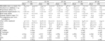
Next we turn to the question whether the effects of these variables on marital fertility are similar in different age groups. Table 6 reports OLS and FE estimates (percentage change) on age-specific marital fertility using the same set of explanatory variables as in Table 5. Generally speaking, the effects grow stronger with increasing age. For child mortality, for example, the FE estimate goes from 4.4 per cent in the age group 20–24 to 6.3 per cent in the age group 40–44, and the effects of the other variables show similar tendencies. The stronger effects in higher age groups are linked to the stronger decline in fertility in higher age groups, as was discussed previously. When societal conditions changed, older women reacted strongest and avoided late childbearing. Most likely this is related to the increased importance of stopping behaviour, or parity-specific control, spreading over the counties as shown earlier. It should be remembered, however, that several variables have significant and sizable effects also in younger age groups, which warns us not to focus attention only on the older women. Apparently, women in all age groups were affected by the changes taking place, and adjusted their behaviour in similar ways but to different degrees.
OLS and fixed-effects panel regression estimates of age-specific marital fertility (percentage change)

***p<0.01, **p<0.05, *p<0.1
Note: The dependent variables are the natural logarithms of age-specific marital fertility.
% effect in y of a one unit change in X is given by 100*(exp(b)-1)).
P-values are based on (White/Huber) heteroskedasticity robust standard errors.
Source: See data appendix.
It is also interesting to note that the negative effect of increasing female relative wages is statistically significant for women over 35, giving some support for the opportunity cost explanation, for which there was no evidence in the total fertility model in Table 5. Changing conditions in the female labour market, with higher relative wages, put a price on the time spent bearing and rearing children, which in turn contributed to the incentive to limit family size. It is only to be expected that this effect should be strongest for older women where the impact of the new stopping behaviour was strongest.
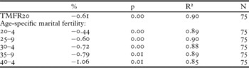
So far we have seen that demand and supply variables seem to have played an important role in the fertility decline in Sweden. This need not imply that other factors could not have been important as well. Despite the relative homogeneity of Swedish society there might have been regional differences in family attitudes, and the great resistance towards the Neomalthusian movement from the 1880s testifies that the attitudes of many people to family limitation were highly traditional (see, e.g., Levin Reference Levin1994). Due to lack of valid quantitative measures of changing attitudes in this period it is only possible to perform a preliminary analysis at this stage. As previously mentioned, voting behaviour has frequently been used as a proxy for modern attitudes in this kind of study, but such information is only available from 1910 onwards. Table 7 shows estimated effects of the proportion voting for socialist parties on marital fertility, both total and age specific, for part of the period of transition (1910–30). The effects are estimated by pooled OLS controlling for the same variables as in the previous tables. The reason for not estimating the FE model in this case is the short period that can be studied due to data availability. Even though these estimates do not tell us much about the impact of change in the voting behaviour on fertility change, they do tell us something about level differences in marital fertility and how they are related to differences in the electorate. There are statistically significant effects of the proportion of socialist voters on both total marital fertility and age-specific marital fertility. A 10-percentage point higher proportion of socialist voters in a county imply about 6 per cent lower marital fertility. The effect also seems considerably stronger among older women. Moreover, the results are highly similar when excluding industrial employment and proportion urban (results not shown), which indicates that they are robust to potential correlation with these variables. Taken together, these results clearly support the hypothesis that attitudes towards birth control, here measured by an admittedly rough proxy, may have been important in the fertility decline, at least if judged by the cross-sectional differences between the counties.
Effects (%) of proportion voting socialist on marital fertility 1910–30

7. Conclusion
Fertility decline in Sweden started around 1880 – about 100 years after the beginning of mortality decline – when marital fertility started to decline continuously. From the evidence presented here it certainly seems as if gradual diffusion of parity-specific control was important in this process, although we have not explicitly analysed the spacing patterns in the decline. The fertility of the oldest age groups declined fastest, even though the decline started in all age groups over 25 at about the same time. In terms of the relative contribution of different age groups to fertility decline it was also the prime childbearing ages 25–40 that contributed most to the decline.
Just before the fertility transition most counties in Sweden did not show any signs of parity-specific control, which implies that, with a few exceptions, the fertility pattern in pre-transitional Sweden can be characterised as natural. Nonetheless, the level of natural fertility varied quite a lot between counties; total marital fertility between 6.7 and 9.3 if the two counties indicating parity-specific control are excluded. These differences not only persisted during the transition but actually widened in relative terms. The relative position (rank) of counties, however, stayed fairly constant, with a few notable exceptions.
The multivariate analysis indicated that several of the variables in the demand-supply framework were associated in the predicted way with marital fertility, although some variables only had an impact on level differences between counties, while others only had an impact through change over time within counties. A higher supply of children following lower child mortality was associated with lower marital fertility. Higher urbanisation and stronger educational orientation were also associated with lower fertility, as they were both related to the higher costs and lower economic benefits of children. Similarly, increasing female relative wages were associated with declining fertility among women over 35, which is consistent with the higher opportunity costs of having children when women's earning potentials increase. These results are also well in line with results for different parts of Germany, using similar types of data and methods of analysis, which stresses the importance of socioeconomic variables in explaining the decline in fertility.
Using age-specific marital fertility data, it could also be demonstrated that older women, in general, adjusted their fertility behaviour more profoundly than younger women, but an important finding was that all age groups were affected by the socioeconomic and demographic changes studied. Although the results give quite strong support to theories of fertility decline emphasising socioeconomic variables as important determinants, attitudes towards birth control may also have played an important role, as shown by the cross-sectional effects of the proportion of socialist voters on marital fertility in all age groups.
Hence, the results presented in this article support an interpretation that connects fertility decline with broad socioeconomic changes taking place in the late nineteenth and early twentieth centuries, following the transition from an agriculturally based economy to an industrial one. This transition involved sustained mortality decline, increasing levels of urbanisation, expansion of education and increased female labour market, and these changes had a profound impact on the demand and supply of children, contributing to widespread fertility control and reduced family size – in other words, to the emergence of the modern two-child family.
Acknowledgements
Financial support from the Swedish Council for Working Life and Social Research (FAS) is gratefully acknowledged. I am grateful to Maria Stanfors for valuable comments and suggestions, and to Christer Lundh for sharing his data with me.
Data appendix
Births by age of mother by civil status. Migration. Deaths of married men: Bidrag till Sveriges Officiella Statistik (BiSOS) A. Befolkningsstatistik 1881–1910. Sveriges Officiella Statistik (SOS). Befolkningsrörelsen 1911–1931.
The population by age, sex and marital status. Rural and urban population. Population distribution by occupation: Bidrag till Sveriges Officiella Statistik (BiSOS) A. Befolkningsstatistik 1880–1910, and Sveriges Officiella Statistik (SOS). Folkräkningen 1910–1930.
Number of teachers and children aged 7–14: Bidrag till Sveriges Officiella Statistik (BiSOS) P. Undervisningsväsendet (Folkskolorna) 1882–1910. Sveriges Officiella Statistik (SOS). Folkskolorna och högre folkskolorna 1919–1920. Sveriges Officiella Statistik (SOS). Folkskolorna 1929–1930.
Agricultural day wages: Bidrag till Sveriges Officiella Statistik (BiSOS) N. Jordbruk och boskapsskötsel 1880–1910 (I am grateful to Christer Lundh for providing this data). Sveriges Officiella Statistik (SOS). Arbetartillgång, arbetstid och arbetslön 1920. Sveriges Officiella Statistik (SOS). Lönestatistisk årsbok 1930.
Industrial wages in Stockholm city 1880–1910: Lundh et al. (Reference Lundh2004); 1920: Bagge (Reference Bagge1933, p. 272); 1930: Sveriges Officiella Statistik (SOS). Lönestatistisk årsbok 1930. Hourly wages in 1920 were transformed to day wages assuming an eight-hour work day (see Isidorsson Reference Isidorsson2002, p. 58).
Cost of living: Myrdal (Reference Myrdal1933) presented a cost of living index for Sweden between 1830 and 1930 based on a relatively large number of products, including for example food, housing and clothing. Since data for many of these commodities are not given for all counties a more limited budget was constructed from the ‘working-class budget’ provided by Myrdal. It contains wheat, rye, barley, oats, potatoes, beef, pork, bacon, butter and eggs. Prices are taken from the data provided by Myrdal and remaining gaps are filled with data from Jörberg (Reference Jörberg1972).
Parliamentary elections: Sveriges Officiella Statistik (SOS). Allmänna val. Riksdagsmannavalen 1909–1911, 1918–1920, 1921, 1929–1932.
Note: BiSOS and SOS are published by Statistics Sweden.