Recording schemes for STEM tomography

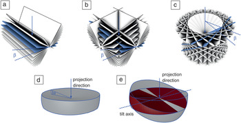
The most commonly used recording scheme for 3D STEM is single-tilt tomography. The specimen is rotated around a single axis perpendicular to the beam direction. Raster-scanned STEM images are then recorded at each tilt angle. The annular dark field (ADF) detector is mostly used to acquire the images, but bright field STEM can be also used. The latter has advantages when imaging thicker specimens because geometric broadening (i.e., the fact that objects at different heights are out of focus) can be reduced with this technique.^{Reference Hohmann-Marriott, Soussa, Azari, Glushakova, Zhang, Zimmerberg and Leapman8} The tilting takes place in either constant angular or slope increments.^{Reference Lee, Fahimian, Iancu, Suloway, Murphy, Wright, Castaño-Díez, Jensen and Miao14} In some cases, samples can be processed to a cylindrical shape, which allows tilting around the full angular range of 360°.^{Reference Palmer and Löwe15} However, many samples have a slab-like geometry as a result of the limitations of the sample preparation procedure or because a wide field of view is required to identify the region of interest. In this case, the tilt range is usually restricted to ±70°. As predicted by the Fourier slice theorem, each projection covers only spatial frequencies that lie on a single plane in frequency space, perpendicular to the projection direction. Intuitively, this means that features perpendicular to the projection direction are preserved, while features in the viewing direction are not captured in the image. As a consequence, the tilt range strongly influences the resolution of the 3D reconstructions,^{Reference Koster, Grimm, Typke, Hegerl, Stoschek, Walz and Baumeister16,Reference Fernandez17} and tomograms from a single-axis tilt series with a limited tilt range suffer from missing information and limited resolution because of this so-called “missing wedge” (Figure 1a).

Figure 1.

Overview of the spatial frequencies covered by different recording schemes. The images show frequencies in Fourier space from the coordinate frame of the sample. The beam direction in the case of an untilted (0°) stage is indicated by a blue arrow. In each image, two adjacent planes are highlighted in blue to annotate the angle between the planes (blue lines). Edges are highlighted using black lines where required for better visibility. (a) Single-axis tilt. (b) Dual-axis tilt. (c) Conical tilt. (d) Focal series. (e) Combined tilt and focal series; the overlapping region between the two tilt directions is marked in red. All tilt angles are annotated with β. For the recording schemes with limited depth of field (d–e), aperture semi-angles are annotated with α. Adapted with permission from References Reference Lanzavecchia, Cantele, Bellon, Zampighi, Kreman, Wright and Zampighi22 and Reference Dahmen, Kohr, de Jonge and Slusallek34. © 2005 Elsevier and © 2009 The Royal Society Publishing, respectively.

A number of different solutions have been explored to reduce or avoid the missing wedge problem. In dual-tilt tomography, two separate tilt series are recorded, whereby one tilt axis is perpendicular to the other tilt axis, and both tilt axes are perpendicular to the beam direction.^{Reference Penczek, Marko, Buttle and Frank18,Reference Mastronarde19} For example, if the beam direction is the z-direction, a dual-tilt series can be realized by first rotating around the x-axis and then around the y-axis to generate a single data set. A dual-tilt series reduces the missing wedge to a missing pyramid (Figure 1b). Dual-axis tilt data sets can be reconstructed by a procedure that independently reconstructs each tilt series and then merges the resulting tomograms in Fourier space^{Reference Mastronarde19} or by using algebraic methods.

Another recording scheme is conical tomography.^{Reference Zampighi, Zampighi, Fain, Wright, Cantele and Lanzaveccia20} The specimen is first rotated around an axis in the lateral plane. The tilt series is then generated by successively tilting around the beam axis (Figure 1c). In this recording scheme, the missing wedge is reduced to a missing cone, leading to isotropic resolution in the x–y plane. A conical tilt series can be reconstructed using tomographic reconstruction methods that work with an arbitrary geometry, such as exact filter methods for general geometry^{Reference Harauz and van Heel21,Reference Lanzavecchia, Cantele, Bellon, Zampighi, Kreman, Wright and Zampighi22} or algebraic methods.

An option to avoid tilting altogether is the recording of a focal series to obtain 3D STEM information.^{Reference Behan, Cosgriff, Kirkland and Nellist23–Reference Frigo, Levine and Zaluzec27} Here, axial information is retrieved from a stack of images with different focal values. The recording scheme is feasible due to the development of spherical aberration correctors, which allow a strongly converging electron beam, and leads to a limited depth of field as a side effect. A focal series captures the part of Fourier space that is equivalent to an inverted double cone (i.e., everything but a double cone in beam direction with an opening angle equal to 90° minus the convergence angle of the beam) (Figure 1d). Therefore, the objective aperture semiangle α is chosen as high as possible in order to achieve the smallest possible depth of field, typically up to approximately 50 mrad (≈2.8°). The focal series data still suffer from a vertically elongated point-spread function (PSF) due to limited sampling in the z-direction.^{Reference Behan, Cosgriff, Kirkland and Nellist23}

A tomographic reconstruction is not required for a focal series, as the data already forms a stack where each image represents one z-slice. However, the 3D data set can be deconvoluted with an approximation of the PSF to remove the blurring effect of the limited depth of field.^{Reference Ramachandra and de Jonge28} Alternatively, the axial elongation of the PSF can be reduced by using a pinhole aperture in the beam path, which removes out of focus information in a similar manner to confocal microscopy.^{Reference Nellist, Cosgriff, Behan and Kirkland29} The latter method has better optical quality than deconvolution, but requires more electron dose. Another option is to align an electron optical path optimized for in-focus information and to scan the stage, instead of the electron beam, in 3D.^{Reference Takeguchi, Hashimoto, Shimojo, Mitsuishi and Furuya30} For a crystalline material with a small sample size, it is possible to obtain the full 3D information from images recorded at just two tilt angles via discrete tomography techniques and estimate the number of atoms per column using statistical methods and the fact that the atomic number contrast of dark-field STEM increases with the number of atoms in a column.^{Reference Van Aert, Batenburg, Rossell, Erni and Van Tendeloo31} Similarly, it is possible to determine the 3D location of small objects such as nanoparticles in an embedding sample from images recorded at a few tilt angles via the parallax equation.

Combined tilt and focal series

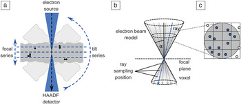
The newest contribution to the set of recording schemes for 3D STEM is the combined tilt and focal series (CTFS).^{Reference Dahmen, Baudoin, Lupini, Kübel, Slusallek and de Jonge32} In this recording scheme, the specimen is rotated in relatively large tilt increments over a limited tilt range, and for every tilt direction, a through-focal series is recorded (Figure 2a). It thus aims to combine the best aspects of the tilt and focus approaches, reduce the missing wedge problem, and limit the tilt range to ±40°, whereby the thickness effect at higher angles remains negligible (the effective thickness increases with 1/cos 40° ≈ 1.3, much less than that for a full tilt series to ±70° with 1/cos 70° ≈ 2.9).

Figure 2.

Schematic overview of the combined tilt and focal series (CTFS) recording scheme. (a) The sample (gray box with indicated black nanoparticles) is tilted by relatively large angular increments, and for every tilt position, a focal series is recorded. (b) The forward projection for the reconstruction of CTFS replaces the line model of the electron beam by a double cone. (c) Lines are placed according to the sampling algorithm stratified rejection sampling.^{Reference Shirley and Marschner33} Considered samples are indicated in blue, rejected samples in white. The results for all lines are averaged to achieve the result for one double cone. Note: HAADF, high-angle annular dark field; α, aperture angle semi-angle.^{Reference Dahmen, Kohr, de Jonge and Slusallek34}

The CTFS captures additional information compared to a tilt series with a large depth of field and leads to a significant reduction of the axial elongation, particularly for thick samples where only a very limited tilt range is accessible (Figure 1e). As with the focal series, a CTFS should be captured with the lowest possible depth of focus. The available tilt range is then covered in tilt increments of at most twice the objective aperture semi-angle, typically ≤5.6°. The reason for this condition is that the Fourier transform of a focal series is nonzero in a set that has the shape of an inverted double cone (i.e., all but a double cone of opening semi-angle 90°-α). This corresponds to a flag structure perpendicular to the beam direction. Thus, as long as this condition is fulfilled, the volume corresponding to the tilt step is covered in reciprocal space (Figure 1e).

Experimental verification

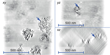
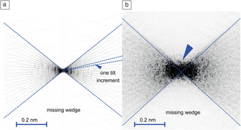
One main issue with pure tilt series-based 3D data due to the missing wedge is lower resolution in the axial direction than in the lateral direction. The CTFS reduces the axial elongation of the PSF such that the resolution in the axial direction becomes closer to that in the lateral direction. This elongation was quantified by experiments on a whole-mount (i.e., unsliced) macrophage cell with embedded gold nanoparticles.^{Reference Dahmen, Baudoin, Lupini, Kübel, Slusallek and de Jonge32} The specimen was imaged using a CTFS, incorporating images from a range of ±40° in 5° increments. For each direction, a focal stack of 20 images in a vertical distance of 50 nm was recorded. The whole data set thus consisted of 340 images. It was shown that the reconstruction obtained from a CTFS could reduce the axial elongation factor from 2.8 ± 0.5 for a pure tilt series to 2.2 ± 0.5 for CTFS, which constitutes a significant (significance level: p < 7.0 × 10^–4) improvement (Figure 3).^{Reference Dahmen, Baudoin, Lupini, Kübel, Slusallek and de Jonge32} The elongation factor describes the ratio of the vertical and the horizontal dimension of the PSF, and thus gives the difference between achieved axial and lateral resolution, respectively. For example, a factor of 2.8 would fit a lateral and axial resolution of 1 nm in the lateral direction and 2.8 nm in the axial direction. This effect was also observed in the Fourier spectrum of the tomogram. In the case of single tilt tomography reconstructed using the simultaneous algebraic reconstruction technique (SART) algorithm, the individual projection directions are clearly visible in the Fourier spectrum of the resulting tomogram, and very little information is computationally reconstructed in the directions corresponding to the missing wedge (Figure 4a). In the case of the CTFS, additional frequencies are present in the region representing the missing wedge (Figure 4b). This additional information was not present in the data set prior to tomographic reconstruction (Figure 1e); in other words, it was obtained computationally by the tomographic reconstruction algorithm.

Figure 3.

Individual slices of a tomogram generated from a combined tilt and focal series of a whole-mount macrophage cell with embedded gold nanoparticles. The tilt range was limited to approximately ±40° due to the sample thickness. The blue arrows indicate the same nanoparticle in all projections. The contrast was inverted to improve the visibility of the nanoparticles.^{Reference Dahmen, Kohr, de Jonge and Slusallek34}

Figure 4.

The frequency spectrum of the reconstructed tomogram. (a) Reconstruction from a single-axis tilt series using the simultaneous algebraic reconstruction technique algorithm. (b) Tomogram of a combined tilt and focal series. The blue arrow marks additional frequencies that are reconstructed by the tomographic reconstruction algorithm.^{Reference Dahmen, Kohr, de Jonge and Slusallek34}

The main advantage of the CTFS thus lies in partial compensation for the missing wedge, which makes the algorithm an advantageous choice for a specimen with a thickness of 1 µm or more, where only a very limited tilt range is accessible. An implementation of the algorithm is available based on the framework Ettention.^{Reference Dahmen, Marsalek, Marniok, Turoňová, Bogachev, Trampert, Nickels and Slusallek35} The open source software is available for Windows and Linux.³⁶ It allows the tomographic reconstruction of data collected by various recording schemes, including CTFS data set. One potential disadvantage of the method is that a large number of projections need to be acquired, which can lead to increased acquisition times and electron doses. It can be conjectured, though, that in the tomographic reconstruction, the noise is averaged over the abundant number of projections, thus the electron dose per image can be reduced.

Future work: Adaptive sampling schemes

We have presented an overview of different homogeneous sampling schemes. All of these schemes are frame-based and static. This means the projection directions are determined by the scheme in advance, and for each direction, one full image is recorded. The images consist of a fixed number of pixels on a Cartesian grid, and every pixel receives the same electron dose. With the emergence of adaptive sampling techniques in the field of FIB/SEM,^{Reference Dahmen, Engstler, Pauly, Trampert, de Jonge, Mücklich and Slusallek37} similar developments can be expected for STEM tomography. Adaptive can hereby mean either of two concepts: (1) an automated microscope will capture data from additional directions as required, based on intermediate representations of the tomogram; or (2) different parts of the image receive a different amount of electron dose, also depending on an analysis of the intermediate data set. The electron dose can then be optimized to capture parts of the image with fine details with a higher dose than areas with a coarser structure, thereby minimizing the electron dose for maximal resolution in the regions where needed.

This acquisition approach results in data sets that have locally varying levels of noise (i.e., contain measurements of nonuniform precision). As the local precision is known (the dose distribution can be retrieved as a separate image showing the individual dwell time of each pixel), this information can be incorporated in the tomographic reconstruction algorithm.