2.1 Experiments

Five steady, uniform flow conditions (denoted as C1 to C5, as listed in table 2) with friction Reynolds number $Re_{\unicode[STIX]{x1D70F}}$ ranging from 614 to 2407 were considered in this study.

Table 2.

Flow conditions. $B$, channel width; $S$, channel slope; $h$, water depth; $B/h$, width-depth ratio; $\unicode[STIX]{x1D708}$, kinematic viscosity; $U_{m}$, depth mean velocity; $u_{\unicode[STIX]{x1D70F}}$, friction velocity, determined based on the log law with von Kármán constant $\unicode[STIX]{x1D705}=0.412$ and additive constant $A=5.29$; $Fr=U_{m}/\sqrt{gh}$, Froude number ($g$ is the gravitational acceleration); $Re=U_{m}h/\unicode[STIX]{x1D708}$, Reynolds number; $Re_{\unicode[STIX]{x1D70F}}=u_{\unicode[STIX]{x1D70F}}h/\unicode[STIX]{x1D708}$, friction Reynolds number.

For the former three lower Reynolds number flow cases (i.e., C1 to C3), the experiments were conducted in a closed recirculating open channel flume with dimensions of 20 m long and 30 cm wide at Tsinghua University, as schematically depicted in figure 1. The channel slope can be changed using the adjustment wheel under the flume. The channel bed and sidewalls are made of ultra-clear glass to facilitate the application of PIV measurements. Honeycombs with decreasing diameters were placed at the entrance of the flume to flatten the flow and remove probable large-scale flow structures generated during the recirculating process. The flume was driven by a pump and the flow rate could be adjusted by changing the motor rotating speed of the pump through a frequency converter. The flow rate was monitored by an electromagnetic flowmeter mounted on the backwater pipe. Eight ultrasonic level sensors were set along the flume to monitor the water depth. The measurement section was located 12 m downstream of the flume entrance to obtain fully developed flow conditions. This distance (approximately $343\sim 480h$) satisfies the criteria documented in the literature, e.g., $76h$ suggested by Kirkgöz & Ardiçlioğlu (Reference Kirkgöz and Ardiçlioğlu1997) and a conservative value of $150h$ suggested by Lien et al. (Reference Lien, Monty, Chong and Ooi2004).

Figure 1.

(a) Schematic diagram of the 20 m long and 30 cm wide open channel flume (not to scale) and (b) corresponding PIV system arrangement and (c) operation mode.

The PIV measurement was conducted in a streamwise wall-normal plane in the middle of the channel. A 1.5 mm-thick laser sheet generated from a pulse laser (Nd:YLF, $20~\text{mJ}~\text{pulse}^{-1}$ at 1 kHz) was used to illuminate the field of view (known as FOV), and a high-speed CMOS camera (IDT Y7-S3, 64GB, $1920\times 1080~\text{pixels}$) was used to capture the particle images. Hollow glass spheres (Dantec Dynamics, HGS-10) with a density of $1.06\times 10^{3}~\text{kg}~\text{m}^{-3}$ and mean diameter of $10~\unicode[STIX]{x03BC}\text{m}$ were used as tracer particles. The pulse laser and camera were synchronized with a digital delay pulse generator (known as DDPG) as demonstrated in figures 1(b) and 1(c). The time interval between the two frames within each image pair, $\unicode[STIX]{x0394}t$, satisfies the one quarter rule (Adrian & Westerweel Reference Adrian and Westerweel2011). The sampling frequency, $F_{s}$, is at $O(1000)~\text{Hz}$ and high enough (with the corresponding time interval between successive velocity field $\unicode[STIX]{x0394}T^{+}<1$) to resolve the small-scale energetic motions. The total image acquisition time $T$, during which the streamwise distance of the mean flow movement $TU_{m}$ was greater than $10\,000h$, is long enough to give convergent spectral results at the largest energetic wavelengths.

As for the latter two highest Reynolds number flow cases (i.e., C4 to C5), the experiments were conducted in a longer and wider recirculating open channel flume at Chongqing Jiaotong University (31 m long, 56 cm wide and 70 cm deep). The bed and sidewalls are also made of glass, for the application of PIV measurements. Three $5~\text{cm}\times 5~\text{cm}$ grids were set at the flume entrance to remove possible large-scale motions. The flow rate and water depth were also monitored by electromagnetic flowmeter and ultrasonic level sensors, respectively. Similar high-frequency and long-duration PIV measurements were performed in the streamwise wall-normal plane at the channel centre, located 16.5 m downstream of the flume entrance to ensure fully developed flow conditions.

Details of the flow conditions and PIV measurement parameters for all the five cases can be seen in tables 2 and 3, respectively. For all cases, the acquired particle images were post-processed with an in-house PIV software using a multipass and multigrid window deformation algorithm which is very similar to that of Scarano (Reference Scarano2002). Accuracy verification of the PIV algorithm can be found in the report of the 4th International PIV Challenge (under the symbol TsU (Kähler et al. Reference Kähler, Astarita, Vlachos, Sakakibara, Hain, Discetti, La Foy and Cierpka2016)). The initial and final interrogation window sizes are $64\times 64$ and $16\times 16$ pixels with an overlap of 50 % with the resulting inner-scaled wall-normal vector spacing $\unicode[STIX]{x0394}y^{+}=5{-}14$.

Table 3.

The PIV parameters: $F_{s}$, the sampling frequency of the velocity fields. Here, $\unicode[STIX]{x0394}T^{+}=\unicode[STIX]{x0394}T/(\unicode[STIX]{x1D708}/u_{\unicode[STIX]{x1D70F}}^{2})$ and $\unicode[STIX]{x0394}TU_{m}/h$, inner- and outer-scaled time interval between successive velocity fields; $T$, total image acquisition time; $\unicode[STIX]{x0394}y^{+}$ (or $\unicode[STIX]{x0394}x^{+}$), the inner-scaled vector spacing in wall-normal (or streamwise) direction.

2.2 Power spectrum

For simplicity of description, $u_{i}$ ($i=1,2$) was adopted to denote the streamwise and wall-normal fluctuating velocity signals with $u_{1}=u$ and $u_{2}=v$. Then the power spectrum (or cross-power spectrum) can be defined as

(2.1)$$\begin{eqnarray}\unicode[STIX]{x1D6F7}_{u_{i}u_{j}}(f)=c|F_{u_{i}}(f)F_{u_{j}}^{\ast }(f)|,\end{eqnarray}$$

where $F_{u_{i}}(f)$ denotes the Fourier transform of fluctuating velocity signal $u_{i}$, $f$ is frequency, superscript $\ast$ indicates the complex conjugate, $|\,|$ designates the modulus, $c$ is a constant determined by satisfying the following equation:

(2.2)$$\begin{eqnarray}\overline{u_{i}u_{j}}=\int _{0}^{\infty }\unicode[STIX]{x1D6F7}_{u_{i}u_{j}}(f)\,\text{d}f.\end{eqnarray}$$

Based on Taylor’s frozen turbulence hypothesis (Taylor Reference Taylor1938), the frequency-based spectrum $\unicode[STIX]{x1D6F7}_{u_{i}u_{j}}(f)$ can be transformed to streamwise wavenumber $k_{x}$ (or wavelength $\unicode[STIX]{x1D706}_{x}$) spectrum $\unicode[STIX]{x1D6F7}_{u_{i}u_{j}}(k_{x})$ (or $\unicode[STIX]{x1D6F7}_{u_{i}u_{j}}(\unicode[STIX]{x1D706}_{x})$) through the following relationships:

(2.3)$$\begin{eqnarray}\left.\begin{array}{@{}c@{}}\displaystyle k_{x}=\frac{2\unicode[STIX]{x1D70B}f}{U(y)},\\ \displaystyle \unicode[STIX]{x1D706}_{x}=\frac{2\unicode[STIX]{x1D70B}}{k_{x}},\end{array}\right\}\end{eqnarray}$$

where $U(y)$ is the mean streamwise velocity at $y$. Even though Taylor’s hypothesis may not be accurate in the low wavenumber range, the errors involved in Taylor’s hypothesis will not corrupt the present results unduly (Kim & Adrian Reference Kim and Adrian1999; Guala et al. Reference Guala, Hommema and Adrian2006). Furthermore, wavenumber spectra derived from Taylor’s hypothesis must reveal less energy at low wavenumber than the true wavenumber spectra, since the time-delayed correlation should decay faster than the two-point correlation due to evolution of the eddy structures as they pass over the measurement point. Therefore, wavenumber spectra in the present paper will be a conservative estimate of the VLSMs.

3.1 Turbulence statistics

Profiles of the mean velocity, turbulence intensity and Reynolds shear stress for all five cases are shown in figure 2. The mean velocity profiles closely follow the direct numerical simulation (DNS) results of closed channel flow (Hoyas & Jiménez Reference Hoyas and Jiménez2008) and exhibit a clear logarithmic distribution (von Kármán constant $\unicode[STIX]{x1D705}=0.412$ and additive constant $A=5.29$, as suggested by Nezu & Nakagawa (Reference Nezu and Nakagawa1993) in open channel flow). The Reynolds shear stress profiles are linearly distributed in the outer layer. Turbulence intensities are consistent with the classical universal functions for open channel flows proposed by Nezu & Rodi (Reference Nezu and Rodi1986). The unique feature relating to the redistribution of turbulent kinetic energy in open channel flows (Komori et al. Reference Komori, Nagaosa, Murakami, Chiba, Ishii and Kuwaharaa1993; Nezu & Nakagawa Reference Nezu and Nakagawa1993; Zhong et al. Reference Zhong, Li, Chen and Wang2015) can be clearly seen in figure 2(b) by comparing the turbulence intensities with those in closed channel flows especially in the near surface region where the free surface restricts and weakens wall-normal turbulence intensity while strengthening the streamwise component. This free-surface induced redistribution of kinetic energy will be discussed further in § 4.3 from a new perspective in terms of VLSMs.

Figure 2.

Wall-normal profiles of turbulence statistical parameters: (a) the mean velocity; (b) turbulence intensity and Reynolds shear stress. von Kármán constant $\unicode[STIX]{x1D705}=0.412$ and additive constant $A=5.29$ are used in the log law (Nezu & Nakagawa Reference Nezu and Nakagawa1993). The DNS results of closed channel flows at $Re_{\unicode[STIX]{x1D70F}}=950$ (CCF950) are from Hoyas & Jiménez (Reference Hoyas and Jiménez2008).

3.2 Uncertainty analysis

For the instantaneous velocity obtained from PIV measurements, the uncertainties mainly originated from the random error in estimating the subpixel location of the correlation peak. This random error is estimated to be less than 0.1 pixel for the present PIV algorithm based on the accuracy verification using 3rd PIV Challenge Case B data, and this uncertainty is consistent with the well documented value of 0.05–0.1 pixels (Westerweel Reference Westerweel1997). Given a mean tracer particle displacement of 8–12 pixels in the present study, this uncertainty accounts for less than 1 % of the real velocity value and shows negligible effects compared to the real velocity fluctuations, based on which this random error would not be considered in the subsequent analysis.

As for the turbulence statistics, they are also affected by the uncertainty. Following the analysis in Sciacchitano & Wieneke (Reference Sciacchitano and Wieneke2016), the uncertainty of the mean velocity (denoted as $\unicode[STIX]{x1D6FF}U$ and $\unicode[STIX]{x1D6FF}V$ for streamwise and wall-normal component, respectively) is given by

(3.1a,b)$$\begin{eqnarray}\unicode[STIX]{x1D6FF}U=\frac{u^{\prime }}{\sqrt{N_{eff}}},\quad \unicode[STIX]{x1D6FF}V=\frac{v^{\prime }}{\sqrt{N_{eff}}},\end{eqnarray}$$

where $u^{\prime }$ and $v^{\prime }$ are the streamwise and wall-normal turbulence intensities, $N_{eff}$ represents the effective number of independent velocity samples and can be obtained through $N_{eff}=T/2T_{int}$ ($T_{int}$ is the integral time scale). The uncertainty of the turbulence intensities ($\unicode[STIX]{x1D6FF}u^{\prime }$ and $\unicode[STIX]{x1D6FF}v^{\prime }$) is

(3.2a,b)$$\begin{eqnarray}\unicode[STIX]{x1D6FF}u^{\prime }=\frac{u^{\prime }}{\sqrt{2(N_{eff}-1)}},\quad \unicode[STIX]{x1D6FF}v^{\prime }=\frac{v^{\prime }}{\sqrt{2(N_{eff}-1)}}.\end{eqnarray}$$

The uncertainty of Reynolds shear stress, $\unicode[STIX]{x1D6FF}\langle uv\rangle$, is obtained by

(3.3a,b)$$\begin{eqnarray}\unicode[STIX]{x1D6FF}\langle uv\rangle =u^{\prime }v^{\prime }\sqrt{\frac{1+\unicode[STIX]{x1D70C}_{uv}^{2}}{N_{eff}-1}},\quad \unicode[STIX]{x1D70C}_{uv}=\frac{\langle uv\rangle }{u^{\prime }v^{\prime }}.\end{eqnarray}$$

In each case, uncertainties of the above turbulence statistics at each $y$ location have been quantified. In summary, the normalized uncertainties by friction velocity are very small ($\unicode[STIX]{x1D6FF}U^{+}<0.03$, $\unicode[STIX]{x1D6FF}V^{+}<0.017$, $\unicode[STIX]{x1D6FF}{u^{\prime }}^{+}<0.022$, $\unicode[STIX]{x1D6FF}{v^{\prime }}^{+}<0.012$, $\unicode[STIX]{x1D6FF}\langle uv\rangle ^{+}<0.036$) and demonstrate that sufficiently large independent velocity samples have been acquired in the present study to obtain reliable turbulence statistics.

3.3 Wavenumber spectrum

For the velocity signals at each wall-normal location, Welch’s overlapped segment averaging method was used to obtain the spectrum. To avoid spectral leakage due to the truncation at the segment edge, a Hamming window was applied for each segment before performing the discrete Fourier transform as advocated by Buxton, de Kat & Ganapathisubramani (Reference Buxton, de Kat and Ganapathisubramani2013). Given that the raw spectrum derived from a raw velocity signal would be contaminated by the high-frequency measurement noise, a 9-point Gaussian kernel with standard deviation of 1.7 was applied to the raw velocity signals to reduce the noise effects. Then, a bandwidth moving filter (BMF) (Baars, Hutchins & Marusic Reference Baars, Hutchins and Marusic2016) of 35 % (meaning that the filtered spectrum at wavenumber $k_{x_{i}}$ is equal to the average of the unfiltered spectrum over span $k_{x_{i}}\pm 35\,\%$) was further adopted to smooth the spectrum to facilitate the identification of bio-peaks of LSMs and VLSMs while not altering the shape of the spectrum.

Figure 3 presents both the raw spectrum (obtained from the raw velocity signal) and filtered spectrum (obtained from the Gaussian filtered velocity signal followed by a 35 % BMF filtering) for streamwise velocity fluctuations at $y/h=0.1$. For comparison, the spectral results in other canonical wall-bounded turbulent flows (pipe, closed channel and TBL) at similar $y$ location and comparable $Re_{\unicode[STIX]{x1D70F}}$ (Kim & Adrian Reference Kim and Adrian1999; Balakumar & Adrian Reference Balakumar and Adrian2007) are also included. The high-frequency measurement noise can be readily seen at high wavenumber range ($k_{x}y>10$, corresponding to a wavelength of $0.06h$ at this $y$ position) of the raw spectrum. The filtering processes adopted here effectively eliminate this inherent high-frequency noise as well as the raw spectrum fluctuations. Good agreement can be observed between the current filtered spectrum and that in other flows, and thereby verifies both the measurement accuracy and the rationality of the post-processing method.

Figure 3.

Wavenumber spectrum for streamwise velocity fluctuation at $y/h=0.1$. Lines are current open channel flow results (dashed lines, raw spectrum obtained from the raw velocity signals; solid lines, filtered spectrum obtained from the Gaussian filtered velocity signals followed by a 35 % BMF filtering). Results of pipe flow (Pipe-1984) are from Kim & Adrian (Reference Kim and Adrian1999) at $Re_{\unicode[STIX]{x1D70F}}=1984$, $y/R=0.084$ ($R$ is the pipe radius). The remaining closed channel and TBL results are from Balakumar & Adrian (Reference Balakumar and Adrian2007): Channel-531, $Re_{\unicode[STIX]{x1D70F}}=531$, $y/h=0.12$ ($h$ is the channel half-height); Channel-960, $Re_{\unicode[STIX]{x1D70F}}=960$, $y/h=0.11$; Channel-1584, $Re_{\unicode[STIX]{x1D70F}}=1584$, $y/h=0.12$; TBL-1476, $Re_{\unicode[STIX]{x1D70F}}=1476$, $y/\unicode[STIX]{x1D6FF}=0.11$ ($\unicode[STIX]{x1D6FF}$ is the boundary layer thickness); TBL-2395, $Re_{\unicode[STIX]{x1D70F}}=2395$, $y/\unicode[STIX]{x1D6FF}=0.11$.

4.1 Premultiplied spectra of streamwise velocity

Following previous studies (Kim & Adrian Reference Kim and Adrian1999; Guala et al. Reference Guala, Hommema and Adrian2006; Adrian Reference Adrian2007; Hutchins & Marusic Reference Hutchins and Marusic2007; Monty et al. Reference Monty, Hutchins, Ng, Marusic and Chong2009), the premultiplied power spectrum of the streamwise velocity, $k_{x}\unicode[STIX]{x1D6F7}_{uu}(k_{x})$, is used to show the streamwise wavelengths associated with LSMs and VLSMs. Premultiplied power spectra across the entire water depth are presented in figure 4, where inner-scale normalization is used in column (i) (left) to highlight the inner layer while outer-scale normalization is used in column (ii) (right) to highlight the outer layer.

Figure 4.

Premultiplied power spectra of streamwise velocity. Inner- and outer-scale normalizations are used in column (i) (left) and column (ii) (right), respectively.

The most noticeable feature in column (i) of figure 4 is the inner peak below the buffer layer ($y^{+}<\sim 30$) with typical wavelength $\unicode[STIX]{x1D706}_{x}^{+}\sim O(1000)$. It is well known that the main energetic structures in the buffer layer are quasi-streamwise vortices (QSVs) (Robinson Reference Robinson1991; Panton Reference Panton2001; Schoppa & Hussain Reference Schoppa and Hussain2002; Jiménez Reference Jiménez2018). These QSVs with typical streamwise extent of 300–400 ($\unicode[STIX]{x1D708}/u_{\unicode[STIX]{x1D70F}}$) can coherently align along the streamwise direction with their transportation roles creating the elongated near-wall streaks with the streamwise extent of ${\sim}O(1000)(\unicode[STIX]{x1D708}/u_{\unicode[STIX]{x1D70F}})$, which is identical to $\unicode[STIX]{x1D706}_{x}^{+}$ of the inner peak in premultiplied power spectra. This result agrees with the conclusion in previous literature that the near-wall cycle of streaks and quasi-streamwise vortices contribute to the strongest peak in premultiplied power spectra (Monty et al. Reference Monty, Hutchins, Ng, Marusic and Chong2009).

As demonstrated in column (ii) of figure 4, the main feature in the outer layer is that there are two dominant and energetic modes (as roughly marked by white dashed lines), which is the same as the double peaks in closed channel and pipe flows (Balakumar & Adrian Reference Balakumar and Adrian2007; Monty et al. Reference Monty, Hutchins, Ng, Marusic and Chong2009). The typical wavelengths of the two modes are around $O(3h)$ and ${\sim}20h$. Thus, they are LSMs and VLSMs, respectively. Comparisons among different cases further show that the energy contained in VLSMs becomes more distinct when the Reynolds number increases, and an outer peak (as marked by black crosses) emerges in C3 to C5 cases despite the peak being very weak in the C3 case. In the two highest Reynolds number cases with $Re_{\unicode[STIX]{x1D70F}}>1800$ (C4, $Re_{\unicode[STIX]{x1D70F}}=1903$; C5, $Re_{\unicode[STIX]{x1D70F}}=2407$), because of the sufficient inner- and outer-scale separation, a clear outer peak can be observed with its wall-normal position located near the centre of log region (i.e., $y^{+}=3.9\sqrt{Re_{\unicode[STIX]{x1D70F}}}$, as highlighted by horizontal black dotted lines), which is similar to that identified in pipe and channel flows (Ng et al. Reference Ng, Monty, Hutchins, Chong and Marusic2011).

Figure 5.

(a) Wavelength of LSMs ($\unicode[STIX]{x1D706}_{xLSMs}$) and VLSMs ($\unicode[STIX]{x1D706}_{xVLSMs}$), represented by small and large symbols, respectively; (b) ratios between $k_{x}\unicode[STIX]{x1D6F7}_{uu}(k_{x})$ at $\unicode[STIX]{x1D706}_{xVLSMs}$ and $\unicode[STIX]{x1D706}_{xLSMs}$; (c) the fraction of kinetic energy carried by VLSMs. In panels (a) and (b), results of different flow types are distinguished by colours (open symbols for present smooth-wall open channel flows (smooth-OCF); closed symbols in different colours are the results of other flow types from the literature) and within each flow type the flow case at different Reynolds numbers are presented with different symbols, as listed in the lower left corner. As for the additional lines, the magenta dashed line in (a) is the empirical formula from Monty et al. (Reference Monty, Hutchins, Ng, Marusic and Chong2009), $\unicode[STIX]{x1D706}_{xVLSMs}=23(y/h)^{3/7}$, and lines in (b) are the linear fitting for the results of different flow types. In (c), results of other flow types are presented with the same symbols as those in (a) and (b) except the present open channel results which are presented by lines (see the legend in panel c) instead of symbols.

4.2 Wavelength, strength and kinetic energy content

For more details, wavelength associated with the LSMs and VLSMs in the premultiplied spectra of streamwise velocity (denoted as $\unicode[STIX]{x1D706}_{xLSMs}$ and $\unicode[STIX]{x1D706}_{xVLSMs}$, respectively) have been identified and compiled in figure 5(a). Additional data extracted from other wall-bounded turbulence studies on pipe flow (Guala et al. Reference Guala, Hommema and Adrian2006), closed channel flow (Balakumar & Adrian Reference Balakumar and Adrian2007), TBL (Balakumar & Adrian Reference Balakumar and Adrian2007) as well as recent studies on rough-wall open channel flows (Cameron et al. Reference Cameron, Nikora and Stewart2017) are also presented for comparison. It should be mentioned here that although the characteristics of VLSMs in rough-wall open channel flows are supposed to be different from those in current smooth-wall conditions, comparisons between the two flow conditions are still meaningful especially for clarifying the potential wall condition effects on the characteristics of VLSMs.

For LSMs, their wavelength $\unicode[STIX]{x1D706}_{xLSMs}$ is roughly the same among different flow scenarios along the whole water depth exhibiting a typical value of $3{-}6h$. However, the wavelength of VLSMs, $\unicode[STIX]{x1D706}_{xVLSMs}$, shows different signatures. Compared to the rough-wall open channel flows, $\unicode[STIX]{x1D706}_{xVLSMs}$ at current smooth-wall conditions is smaller. This can be speculated and explained as follows: the roughness Reynold number in Cameron et al. (Reference Cameron, Nikora and Stewart2017) is $D^{+}=605$ ($D$ is the diameter of the roughness elements) and indicates a fully rough-flow condition. These rough elements seem to be big enough to restrict the inherent meandering feature of VLSMs, based on which a longer wavelength of VLSMs can be captured from a fixed-point measurement. Given the finite size of these roughness elements, the above speculated roughness effects are expected to be weakened when the water depth increases, i.e., the submergence of the rough elements increases. As can be seen in figure 5(a), $\unicode[STIX]{x1D706}_{xVLSMs}$ in rough wall open channel flows will decrease and tend to follow our smooth-wall results when the Reynolds number increases (realized by increasing the water depth, or in other words, increasing the submergence of the rough elements given that $D^{+}$ is fixed ($D^{+}=605$) in Cameron et al. (Reference Cameron, Nikora and Stewart2017)), this observation provides strong support for the above speculation. When compared with other canonical wall-bounded turbulent flows (pipe, closed channel and TBL), although the wavelength of VLSMs in present smooth-wall open channel flows shows a comparable value, their presence extends further away from the wall and can almost extend to the free surface.

Figure 5(b) further shows the relative strength relationship between VLSMs and LSMs in different flow types by plotting the ratios between $k_{x}\unicode[STIX]{x1D6F7}_{uu}(k_{x})$ at $\unicode[STIX]{x1D706}_{xVLSMs}$ and $\unicode[STIX]{x1D706}_{xLSMs}$. When there were no distinct peaks at a given $y$ position, $k_{x}\unicode[STIX]{x1D6F7}_{uu}(k_{x})$ values at $3h$ and $15h$ were adopted as the surrogates. Although data points are relatively scattered, we can also find out the different trends among different flow types within experimental uncertainty. The strength of VLSMs compared with LSMs at the same $y$ position in closed channel, pipe and TBL is always reducing beyond $y/h=0.5$, which could be roughly demonstrated by the negative slope of the linear fitting lines as shown in figure 5(b). The slopes of the linear fitting lines for closed channel, pipe and TBL are $-0.26$, $-1.03$ and $-0.93$, respectively. At $y/h=0.8$, the $k_{x}\unicode[STIX]{x1D6F7}_{uu}(k_{x})$ for VLSMs is approximately 70 %, 50 % and 35 % of that for LSMs in closed channel, pipe and TBL, respectively. However, this ratio remains greater than 90 % beyond $y/h=0.5$ in open channel flows both at smooth- and rough-wall conditions given the slower decreasing trends (the negative slopes are $-0.12$ and $-0.11$ for smooth- and rough-wall open channel, respectively), and indicates that VLSMs maintain the comparable strength with LSMs in the outer and near surface region.

Following the widely adopted separation scale value in the literature (Guala et al. Reference Guala, Hommema and Adrian2006; Balakumar & Adrian Reference Balakumar and Adrian2007), $\unicode[STIX]{x1D706}_{x}=3h$ was used here to separate LSMs and VLSMs. Then the contributions of VLSMs to turbulence intensity, or equivalently the fraction of energy carried by VLSMs, can be defined as

(4.1)$$\begin{eqnarray}\unicode[STIX]{x1D6FE}_{uu}=\frac{\displaystyle \int _{0}^{2\unicode[STIX]{x1D70B}/3h}\unicode[STIX]{x1D6F7}_{uu}(k_{x})\,\text{d}k_{x}}{\displaystyle \int _{0}^{\infty }\unicode[STIX]{x1D6F7}_{uu}(k_{x})\,\text{d}k_{x}}.\end{eqnarray}$$

The variation in $\unicode[STIX]{x1D6FE}_{uu}$ as a function of $y/h$ is shown in figure 5(c), where results from other wall-bounded flows are also included for comparison. In the outer region of open channel flows (e.g., $y/h>0.15\sim 0.2$) where VLSMs dominate, $\unicode[STIX]{x1D6FE}_{uu}$ is $0.5\sim 0.65$ and indicates that VLSMs contribute to over 50 % of the streamwise turbulence intensity, which is consistent with the reported value in pipe (Guala et al. Reference Guala, Hommema and Adrian2006) and closed channel flows (Balakumar & Adrian Reference Balakumar and Adrian2007) while greater than that in turbulent boundary layers (Balakumar & Adrian Reference Balakumar and Adrian2007). As discussed by Balakumar & Adrian (Reference Balakumar and Adrian2007) and Monty et al. (Reference Monty, Hutchins, Ng, Marusic and Chong2009), the variations in the streamwise kinetic energy carried by the VLSMs in different wall-bounded turbulent flows may be induced by the difference of flow geometry.

4.3 Free surface effects and relations to TKE redistribution

To clarify the free surface effects relating to VLSMs, comparisons are made between open channel and closed channel flows in this subsection, as the only difference between them is the upper boundary.

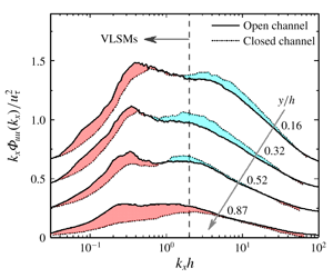
As has been documented for quite a long time, compared to closed channel flow, the presence of free surface in open channel will result in the redistribution of TKE (i.e., reduction of wall-normal fluctuations while strengthening the streamwise and spanwise ones). This TKE redistribution can be readily seen in figure 6(a), where the open channel flow shows a higher streamwise turbulence intensity than closed channel in the outer region at comparable Reynolds number. Given that the turbulence intensity is a statistical reflection of the inherent turbulence structures, the turbulence intensity difference implies a strong free surface effect on the turbulence structures.

Figure 6.

Comparison of streamwise turbulence intensity (a) and premultiplied spectra (b,c) with closed channel flow at comparable Reynolds numbers. Solid lines are from C3 case, $Re_{\unicode[STIX]{x1D70F}}=1508$, $Fr=1.43$; dash-dotted lines are from C4 case, $Re_{\unicode[STIX]{x1D70F}}=1903$, $Fr=0.91$; dashed lines are the data from closed channel flows: data in (a) are from Hoyas & Jiménez (Reference Hoyas and Jiménez2008), $Re_{\unicode[STIX]{x1D70F}}=2000$, and in (b,c) is from Balakumar & Adrian (Reference Balakumar and Adrian2007), $Re_{\unicode[STIX]{x1D70F}}=1584$. The lines in (b,c) from top to bottom are the premultiplied power spectra at $y/h=0.16$, 0.32, 0.52 and 0.87, respectively (as marked in panel a), with 0.2 added on each higher line. Shaded regions represent the difference between the curves of open channel and closed channel, with red and blue representing higher and lower value region in open channel flows.

To see what structure difference the free surface results in, the premultiplied spectra $k_{x}\unicode[STIX]{x1D6F7}_{uu}(k_{x})$ at multiple $y$ positions ($y/h=0.16$, 0.32, 0.52 and 0.87) are compared between closed channel and present open channel flows at comparable Reynolds numbers (see figures 6b and 6c), among which the spectral results of closed channel flow ($Re_{\unicode[STIX]{x1D70F}}=1584$) are from Balakumar & Adrian (Reference Balakumar and Adrian2007). For the results of open channel flows, both C3 ($Re_{\unicode[STIX]{x1D70F}}=1508$, $Fr=1.43$, corresponding to the supercritical flow condition) and C4 ($Re_{\unicode[STIX]{x1D70F}}=1903$, $Fr=0.91$, corresponding to the subcritical flow condition) cases are presented to consider the potential Froude number effect. It should be noted here that the spectral curves in figures 6(b) and 6(c) for $y/h=0.16$, 0.32, 0.52 and 0.87 are shown from top to bottom with 0.2 added on each higher line. And the corresponding $y$ positions were marked with arrows in figure 6(a) to show the turbulent intensity difference at corresponding positions. For a better demonstration of the difference, the regions between the curves of open and closed channel flows are coloured, where red and blue regions denote higher and lower values in open channel, respectively.

As demonstrated in figure 6(b), in the near-wall positions (e.g., $y/h=0.16$ and 0.32), even though the area under open and closed channel curves is roughly the same given the turbulence intensities of the two flows are identical therein, the curves shape is slightly different, i.e., higher $k_{x}\unicode[STIX]{x1D6F7}_{uu}(k_{x})$ values in the low wavenumber range while lower $k_{x}\unicode[STIX]{x1D6F7}_{uu}(k_{x})$ values in the high wavenumber range of open channel flows as indicated by red and blue regions, respectively. This difference could be caused by some real and physical structure difference, but also could be an artificial difference resulting from the error in the integration and normalization process. More detailed comparative studies need to be carried out before we can come to a certain conclusion. Moving away from the wall, the area under the curves of open channel flow becomes bigger than that of closed channel flow because of the higher turbulence intensity in open channel flows. In addition, the curves of the two flow types tend to become identical in the high wavenumber range which could be seen from the vanishing of the blue region. It is also quite clear that extra area in open channel flows near the free surface (see the curves for $y/h=0.87$) mostly resides within the low wavenumber region. By checking the wavenumber, it can be readily known that this extra area is mostly contributed by VLSMs. The above spectral difference between closed and open channel flows presents at both supercritical (C3 case, see figure 6b) and subcritical (C4 case, see figure 6c) flow conditions with no observable difference seen between the two flow regimes, at least within the Froude number range considered in this study ($(0.8{-}0.91)<Fr<1.43$). More systematic experiments that cover a much wider Froude number range are needed to see whether any Froude number effect presents therein.

Combining the results in § 4.2 and figure 6, it can be readily seen that the free surface seems to sustain/promote the development and survival of VLSMs which in turn results in their further presence and higher strength in the outer layer of open channel. Despite the causality between the TKE redistributions and VLSMs still being unclear, the spectral difference between open channel and closed channel flows in the near surface region, which are almost all contributed from VLSMs, gives a strong indication of the close relationship between VLSMs and TKE redistributions.