INTRODUCTION
Wiggle matching is a powerful technique used in radiocarbon dating to improve the precision with which one can estimate calendar ages of samples (Pearson Reference Pearson1986). The classic usage of the technique is when seeking to estimate the calendar ages of a series of tree-ring samples for which, due to ring counting, the number of calendar years separating the samples is known precisely. By calibrating multiple determinations jointly within a wiggle match we can improve the precision in our absolute calendar age estimates compared with the estimate we would obtain with just a single determination.
Suppose we are dating such a tree-ring sequence consisting of N determinations from consecutive annual rings, such that we know that the true, calendar ages must be
 ${T_1},{T_2} = {T_1} + 1,{T_3} = {T_1} + 2, \ldots ,{T_N} = {T_1} + N - 1$
. Given
 ${T_1}$
, all the other ages are known and so this is the only unknown we need to estimate. We obtain radiocarbon data for each tree ring, and then try to match the ups and downs in the data to ups and downs in the calibration curve, knowing that we have N consecutive years.
Bayesian theory has been applied to make this method quantitative, (see for example Christen and Litton Reference Christen and Litton1995; Bronk Ramsey et al. Reference Bronk Ramsey, van der Plicht and Weninger2001). The net result is an expression, in terms of the data, for
 $p({T_1} = {t_1}|data)$
, the probability for the unknown age
 ${T_1}$
given the set of N radiocarbon determinations. This expression is also dependent upon the value of the calibration curve
 $\mu ({t_1}), \ldots ,\mu ({t_1} + N - 1)$
. The formulae given in these papers assume pointwise estimates of the calibration curve which are independent from one another and ignore any potential covariance information between the estimates at adjacent times.
The importance of such covariance structure in the calibration curve has long been understood, see for example Blackwell and Buck (Reference Blackwell and Buck2008) and Millard (Reference Millard2008). Millard (Reference Millard2008) discusses wiggle matching and covariance, and provides results of several wiggle matching calculations which incorporate the covariance information from the calibration curve.
Our goal in this brief note is to derive a generalization of the usual Bayesian wiggle-match formulation for
 $p({T_1} = {t_1}|data)$
, to show how this result is modified by the covariance effects under the assumption that the calibration curve is modelled as a multivariate normal distribution. Our final answer, a new expression for
 $p({T_1} = {t_1}|data)$
, is given by Equations (8)–(10). It has the same general structure as the usual formula, and it explicitly shows how the covariance information from the calibration curve enters into the result. The next section contains our derivation. As much as possible, we use the approach and notation already developed for this type of analysis — for examples, see Heaton et al. (Reference Heaton, Blackwell and Buck2009, Reference Heaton, Blaauw, Blackwell, Bronk Ramsey, Reimer and Scott2020), Bronk Ramsey (Reference Bronk Ramsey2015), Niu et al. (Reference Niu, Heaton, Blackwell and Buck2013), and Blackwell and Buck (Reference Blackwell and Buck2008).
BAYESIAN THEORY
We denote the true, unknown calendar ages of our N samples by
 $\{ {T_i}\} _{i = 1}^N$
, and the observed radiocarbon determinations (either radiocarbon ages or
 $^{14}$
C/
 $^{12}$
C ratios) by
 ${\bf{y}} = ({y_1}, \ldots ,{y_n}{)^T}$
. We denote the unknown true value of the calibration curve (either the true radiocarbon age or
 $^{14}$
C/
 $^{12}$
C ratio for calendar age t cal BP) in any calendar year by
 $\mu (t)$
. Thus, we have
 $$p({y_i}|{T_i} = {t_i},\mu ({t_i})) = {1 \over {\sqrt {2\pi \sigma _i^2} }}\exp \left( - {{{{({y_i} - \mu ({t_i}))}^2}} \over {2\sigma _i^2}}\right),$$
where
 ${\sigma _i}$
is the uncertainty in the radiocarbon measurement. We do not know the true value of the calibration curve (i.e., the true value of radiocarbon age or
 $^{14}$
C/
 $^{12}$
C ratio corresponding to calendar age t cal BP) but we do have pointwise estimates
 $\hat \mu (t)$
in any given year, so that we have
 $\mu (t)= \hat \mu (t) + \epsilon (t).$
The
 $\epsilon (t)$
denotes our uncertainty in the calibration curve at time t. Typically there will be covariance in these values —
 $\epsilon (t)$
will not be independent of
 $\epsilon (t + 1)$
. If we assume that these uncertainties have a multivariate Gaussian form and consider any sequence of N consecutive calendar years
 ${\bf{t}} = (t,t + 1, \ldots ,t + N - {1)^T}$
:
 $$p({\epsilon _t}) = (2\pi {)^{ - N/2}}\det {({\Sigma _t})^{ - {1 \over 2}}}\exp \left( { - {1 \over 2}\epsilon _t^T\Sigma _t^{ - 1}{\epsilon _{\bf{t}}}} \right),$$
where
 ${\epsilon _t} = (\epsilon (t), \ldots ,\epsilon (t + N - {1))^T}$
and
 ${\sum _t}$
is the covariance matrix which encodes the correlations in the
 ${\epsilon _t}$
uncertainties, and in general will depend on t. According to Equation (2), for any vector of calendar ages
 ${\bf{t}}$
, we have
 ${\mu _t} = {{\hat \mu}_t} + {\epsilon _t}.$
Here
 ${\mu _t}$
denotes the vector of true radiocarbon ages or
 $^{14}$
C/
 $^{12}$
C ratios (to correspond to choice of the
 ${y_i}$
’s) for the sequence of calendar age
 ${\bf{t}}$
, and
 ${{\hat \mu}_t}$
the corresponding pointwise estimates.
We are now ready to begin our derivation. We first note that the quantity we want is
 $f({t_1}) = p({T_1} = {t_1}|data) = p({T_1} = {t_1}|{\bf{y}})$
. To calculate this we use Bayes’ Theorem:
 $f({t_1}) = p({T_1} = {t_1}|data) = p({T_1} = {t_1}|{\bf{y}}) = ap({\bf{y}}|{t_1}){\pi _0}({t_1})$
Here, a is a normalization constant, and
 ${\pi _0}({t_1})$
is the prior probability for
 ${T_1}$
. We expand
 $p({\bf{y}}|{t_1})$
to obtain (to save writing, we denote
 ${t_j} = {t_1} + j - 1$
, the calendar age of the
 ${j^{th}}$
determination in the sequence to be wiggle-matched)
 $$\matrix{
{f({t_1}) = a\int \ldots \int [ \left\{ {\prod\limits_{j = 1}^N {\int p } ({y_j}|{t_1},\mu ({t_j}))p(\mu ({t_j})|{t_1},({t_j}))d\mu ({t_j})} \right\}} \cr
{ \times p(({t_1}), \ldots ,({t_N})|{t_1}){\pi _0}({t_1})]d({t_1}) \ldots d({t_N}),} \cr
} $$
We note that
 $p(\mu ({t_j})|{t_1},\epsilon ({t_j})) = \delta (\mu ({t_j}) - \hat \mu ({t_j}) - \epsilon ({t_j}))$
, where
 $\delta ()$
is the Dirac delta function. Thus we have
 $$\matrix{
{f({t_1}) = a\int \ldots \int [ \left\{ {\prod\limits_{j = 1}^N {\int {\exp } } \left( { - {{{{({y_j} - \mu ({t_j}))}^2}} \over {2\sigma _j^2}}} \right)\delta (\mu ({t_j}) - \hat \mu ({t_j}) - ({t_j}))d\mu ({t_j})} \right\}} \cr
{ \times p(({t_1}), \ldots ,({t_N})|{t_1}){\pi _0}({t_1})]d({t_1}) \ldots d({t_N}).} \cr
} $$
Note that we keep absorbing into the normalization constant a those factors that do not depend on
 ${t_1}$
. Doing the integral over
 $\mu ({t_1}), \ldots ,\mu ({t_N})$
gives
 $$\matrix{
{f({t_1}) = a\int \ldots \int {\left[ {\exp \left( { - \sum\limits_{j = 1}^N {{{{{({y_j} - \hat \mu ({t_j}) - ({t_j}))}^2}} \over {2\sigma _j^2}}} } \right)} \right.} } \cr
{ \times \det {{({\Sigma _{{t_1}}})}^{ - {1 \over 2}}}\exp \left( { - {1 \over 2}_t^T\sum\limits_t^{ - 1} {{_t}} } \right){\pi _0}({t_1})]d({t_1}) \ldots d({t_N}).} \cr
} $$
Finally, we do the integral over the
 $\epsilon ({t_1}), \ldots ,\epsilon ({t_N})$
to get
 $$f({t_1}) = a\sqrt {{{\det (\sum _{{t_1}}^{ - 1})} \over {\det ({{\textbf T}_{{t_1}}})}}} \exp \left( { - {1 \over 2}{{({{\hat \mu }_{{t_1}}} - y)}^T}{{\boldsymbol W}_{{t_1}}}({{\hat \mu }_{{t_1}}} - y)} \right){\pi _0}({t_1}).$$
This is our final answer; it is similar to usual Bayesian result in being a multivariate Gaussian in
 ${{\hat \mu}_{{t_1}}} - {\bf{y}}$
. However, it now involves the
 $N \times N$
matrix
 ${\boldsymbol{{W}}_{{t_1}}}$
, which in general has off-diagonal terms. This matrix is given by
 $${\left[ {{W_{{t_1}}}} \right]_{ij}} = {1 \over {\sigma _i^2}}{\delta _{ij}} - {1 \over {\sigma _i^2\sigma _j^2}}{\left[ {T_{{t_1}}^{ - 1}} \right]_{ij}} \quad\quad{\left[ {{T_{{t_1}}}} \right]_{ij}} = {\left[ {\Sigma _{{t_1}}^{ - 1}} \right]_{ij}} + {1 \over {\sigma _i^2}}{\delta _{ij}}.$$
In general these matrices, as well as the determinants of
 $\sum _{{t_1}}^{ - 1}$
and
 ${\boldsymbol{{T}}_{{t_1}}}$
, will depend on
 ${t_1}$
.
The matrix
 ${\boldsymbol{{W}}_{{t_1}}}$
can be written in a more compact, elegant form. If we define a diagonal matrix
 ${D_{ij}} = \sigma _i^2{\delta _{ij}}$
, containing the variances of the radiocarbon determinations
 ${\bf{y}}$
on the diagonal, then we may write
 ${\boldsymbol{{W}}_{{t_1}}} = (\boldsymbol{{D}} + {\sum _{{t_1}}}{)^{ - 1}}.$
To derive this, we can go back to Equation (4), and evaluate
 $p({\bf{y}}|{t_1})$
in the following way. We note that the N-dimensional random variable
 ${\bf{y}} - {{\hat \mu}_{{t_1}}}$
can be viewed as the sum of two, independent, multivariate Gaussians, each with a mean of zero, and with covariance matrices given by
 ${\sum _{{t_1}}}$
and by
 $\boldsymbol{{D}}$
. It is well known that the probability density of this sum is itself a Gaussian, with a covariance matrix given by
 $\boldsymbol{{D}} + {\sum _{{t_1}}}$
. The equivalence of these two forms for
 ${\boldsymbol{{W}}_{{t_1}}}$
, given in Equations (9) and (10), is shown in the Appendix.
SPECIAL CASES
Certain special cases are instructive. First, suppose that there are no correlations among the
 $\epsilon ({t_j})$
. This implies that
 $\sum $
is a diagonal matrix:
 ${\Sigma _{ij}} = s_j^2{\delta _{ij}}$
Thus,
 $s_j^2$
is the variance in the calibration curve at time
 ${t_j}$
. It is then straightforward to show that the
 $\boldsymbol{{W}}$
matrix becomes
 $${W_{ij}} = {1 \over {\sigma _j^2 + s_j^2}}{\delta _{ij}}$$
This is the usual Bayesian result (Christen and Litton Reference Christen and Litton1995; Bronk Ramsey et al. Reference Bronk Ramsey, van der Plicht and Weninger2001), which we recover for this case; any differences in
 $\boldsymbol{{W}}$
from this usual result thus are totally due to correlations among the
 $\epsilon ({t_j})$
.
Another special case to consider is if the radiocarbon determinations are very precise, so that all of our uncertainty comes from the calibration curve, Taking
 ${\sigma _j} \to 0$
then gives
 $\boldsymbol{{W}} = \sum _t^{ - 1}$
. The Gaussian in the wiggle matching formula (8) then directly reflects the covariance matrix from the calibration curve.
ROLE OF THE COVARIANCE MATRIX
 $\Sigma $

It is perhaps not easy to understand the role played in the wiggle matching equation by the off-diagonal elements of the covariance matrix
 ${\Sigma _{ij}}$
; these would be
 ${\rm{Cov}}(\epsilon ({t_i}),\epsilon ({t_j}))$
for
 $i \ne j$
. To gain some insight, we can consider the following special case: suppose that the off-diagonal elements of
 $\Sigma $
are much smaller than the diagonal elements. Thus we write
 ${\Sigma _{ij}} = s_i^2{\delta _{ij}} + {G_{ij}}$
where
 ${G_{ij}} = 0$
for
 $i \ne j$
. If we now assume that the elements of G are small compared to the diagonal elements, we can derive the following result: to first order in G we have
 $${W_{ij}} \approx {1 \over {\sigma _j^2 + s_j^2}}{\delta _{ij}} - {{{G_{ij}}} \over {\Big(\sigma _i^2 + s_i^2\Big)\Big(\sigma _j^2 + s_j^2\Big)}}$$
The effect of the diagonal first term is clear: when inserted into Equation (8) it will assign higher probabilities to values of
 ${t_1}$
which make the magnitudes of the various
 ${y_i} - \hat \mu ({t_i})$
as small as possible. The second, off-diagonal term will favor values of
 ${t_1}$
which cause the various products
 $({y_i} - \hat \mu ({t_i}))({y_j} - \hat \mu ({t_j}))$
to have the same sign as
 ${G_{ij}}$
. Thus, if, for example,
 ${G_{23}}$
is positive, the off-diagonal term will favor values of
 ${t_1}$
which make
 $({y_2} - \hat \mu ({t_2}))({y_3} - \hat \mu ({t_3}))$
positive.
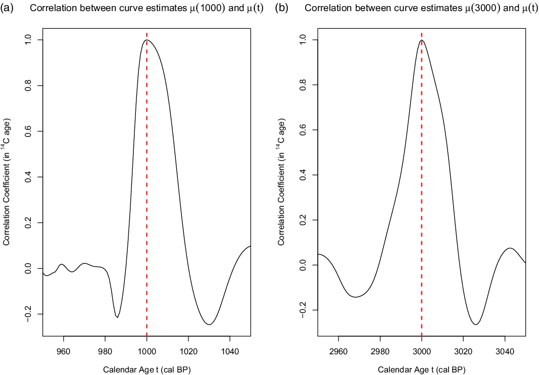
To give some sense of how large the off-diagonal terms can be, we present examples of the correlations in the IntCal20 curve, and how they decay as the distance between calendar ages increases. In Figure 1 we plot the correlation between
 $\mu (t)$
and
 $\mu ({t^ \star })$
for
 ${t^ \star } = 1000$
, and for
 ${t^ \star } = 3000$
cal BP. In terms of our present notation, the correlation function
 $C(t,{t^ \star })$
plotted is given by
 $$C(t,{t^ \star }) = {{\lt \epsilon (t)\epsilon ({t^ \star })\gt } \over {\sqrt {\lt{\epsilon ^2}(t)\gt \lt{\epsilon ^2}({t^ \star })\gt}}}$$
An illustration of the correlation in the IntCal20 calibration curve. Panel (a) shows the correlation between the value of the calibration curve at 1000 cal BP, i.e.
 $\mu (1000)$
, and
 $\mu (t)$
for
 $950 \le t \le 1050$
(50 calendar years either side). Panel (b) the correlation between
 $\mu (3000)$
and
 $\mu (t)$
, for
 $2950 \le t \le 3050$
. The quantity plotted on the y-axis is given by Equation (15).

where the brackets indicate the expectation over the random variables
 $\epsilon (t)$
.
We see that the off-diagonal terms are comparable to the diagonal ones over about 10–20 years in both cases; thus, over the range of a short wiggle-match (ca. 20 calendar years), correlations can be significant.
Discussion
We have discussed a generalization of the usual Bayesian approach to wiggle matching. The key ingredients in this formulation are the pointwise mean estimates of the calibration curve
 $\hat \mu (t)$
, and the corresponding curve covariance which for any set of N consecutive years we assume can be encoded in an
 $N \times N$
covariance matrix
 $\sum $
. As we have shown, information about these quantities can be provided by the constructors of the calibration curve; for relevant discussion of the newly presented calibration curves, see, for example Heaton et al. (Reference Heaton, Blaauw, Blackwell, Bronk Ramsey, Reimer and Scott2020), Reimer et al. (Reference Reimer, Austin, Bard, Bayliss, Blackwell, Ramsey, Butzin, Cheng, Edwards, Friedrich, Grootes, Guilderson, Hajdas, Heaton, Hogg, Hughen, Kromer, Manning, Muscheler, Palmer, Pearson, van der Plicht, Reimer, Richards, Scott, Southon, Turney, Wacker, Adolphi, Büntgen, Capano, Fahrni, Fogtmann-Schulz, Friedrich, Köhler, Kudsk, Miyake, Olsen, Reinig, Sakamoto, Sookdeo and Talamo2020), and van der Plicht et al. (Reference van der Plicht, Bronk Ramsey, Heaton, Scott and Talamo2020).
The ultimate origins of the correlated uncertainties in the calibration curve (the off-diagonal elements of
 ${\Sigma _{ij}}$
) should perhaps be discussed. When constructing the radiocarbon calibration curve, we assume that the underlying curve
 $\mu (t)$
one is trying to estimate is somewhat smooth, i.e., that the level of
 $^{14}$
C in the atmosphere in calendar year t is similar to that in year
 $t + 1$
. This is the basis of most statistical regression techniques and means that information on the value of the curve in one calendar year also informs us about what its value is likely to be in neighbouring years. In our case it is supported by our knowledge about the nature of the carbon cycle. Indeed, it is this assumption of smoothness which allows us to borrow and combine information from multiple
 $^{14}$
C observations over a neighborhood to strengthen the curve estimate in any individual year and prevent overfitting to the data. Without it, we could make no prediction about the value in a calendar year for which there was no direct observation.
This smoothness creates a level of dependence in the resultant curve estimate that provides more information than, and goes beyond, just the pointwise intervals for
 $\hat \mu (t)$
. It is unlikely that the true atmospheric
 $^{14}$
C levels will flip from the top of the curve’s probability interval to the bottom in the space of a single year. Rather if the true value of the curve lies towards the top (bottom) of the probability interval in year t, it is likely to also lie towards the top (bottom) of the interval in nearby times
 $t'$
. In our notation,
 $\epsilon (t)$
and
 $\epsilon (t')$
are likely to have the same sign when
 $t'$
is in the neighbouhood of t.
The level of smoothness, and hence dependence, in the calibration curve will be affected by the nature of the reference
 $^{14}$
C data used to construct the calibration curve (to which we aim to adapt) and, in the case of IntCal20, the number and placement of the knots in the underlying spline. Over time spans with a lower density of knots, the resulting estimate for the calibration curve will however be smoother, and this will tend to create longer lasting curve covariance. There are also specific times, during solar proton (SPE or Miyake) type events, where the smoothness of the IntCal curve is permitted to be reduced.
The diverse nature of the
 $^{14}$
C data used to construct the IntCal curve will also influence the covariance in the final calibration curve estimate. In particular, in the older portion of the calibration curve (
 $\! \gt 14,\!000$
cal yr BP) the calendar ages and
 $^{14}$
C measurements of the reference data themselves exhibit significant covariance. Here the calibration curve is informed by
 $^{14}$
C measurements from floating tree-ring sequences (Adolphi et al. Reference Adolphi, Muscheler, Friedrich, Guttler, Wacker, Talamo and Kromer2017; Turney et al. Reference Turney, Fifeld, Hogg, Palmer, Hughen, Baillie, Galbraith, Ogden, Lorrey, Tims and Jones2010, Reference Turney, Palmer, Bronk Ramsey, Adolphi, Muscheler, Hughen, Staff, Jones, Thomas, Fogwill and Hogg2016) for which the internal chronologies are known, but the absolute ages are not — these are adaptively wiggle-matched, during curve construction, to fit with the rest of the reference
 $^{14}$
C data. The calendar ages of the macrofossils from Lake Suigetsu (Bronk Ramsey et al. Reference Bronk Ramsey, Heaton, Schlolaut, Staff, Bryant, Brauer, Lamb, Marshall and Nakagawa2020) also possess covariance, as do the foraminifera from ocean sediments (Bard et al. Reference Bard, Menot, Rostek, Licari, Boning, Edwards, Cheng, Wang and Heaton2013; Hughen and Heaton Reference Hughen and Heaton2020) which are linked to the Hulu Cave timescale by the tying of global abrupt palaeoclimatic events (Heaton et al. Reference Heaton, Bard and Hughen2013). The speleothem
 $^{14}$
C measurements (e.g., Cheng et al. Reference Cheng, Lawrence Edwards, Southon, Matsumoto, Feinberg, Sinha, Zhou, Li, Li and Xu2018; Southon et al. Reference Southon, Noronha, Cheng, Edwards and Wang2012) share a common dead carbon fraction; and the marine based
 $^{14}C$
measurements (e.g., Bard et al. Reference Bard, Menot, Rostek, Licari, Boning, Edwards, Cheng, Wang and Heaton2013; Hughen and Heaton Reference Hughen and Heaton2020) also share a
 $^{14}$
C offset due to the modelling of the marine reservoir age (Butzin et al. Reference Butzin, Heaton, Kohler and Lohmann2020). All these covariances within the constituent IntCal reference data will affect, and tend to increase, the covariance on the final curve estimate
 $\hat \mu (t)$
in this time period, see Heaton et al. (Reference Heaton, Blaauw, Blackwell, Bronk Ramsey, Reimer and Scott2020) for details.
Acknowledgments
This work was supported by National Science Foundation grant EAR 0112480 and a Leverhulme Trust Fellowship RF-2019-140\ 9. We are grateful to a reviewer whose thoughtful comments motivated us to discuss the nature and origin of the covariance effects.
APPENDIX
We want to prove that the two expressions (9) and (10) given for the matrix W are equivalent. The normalising constant obtained in (8) can also be shown to be equivalent to the approach using the result that the sum of two multivariate Gaussians is Gaussian, although we do not show this here. In this Appendix, all the symbols represent
 $N \times N$
matrices, so we omit the bold face notation. The two forms are:
 ${W_A} = {D^{ - 1}} - {D^{ - 1}}{({\Sigma ^{ - 1}} + {D^{ - 1}})^{ - 1}}{D^{ - 1}}\qquad {W_B} = (D + \Sigma {)^{ - 1}}$
where D and
 $\Sigma $
are defined in the main text.
 ${W_A}$
is the form given by Equation (9), while
 ${W_B}$
is the form given by Equation (10). It is sufficient to show that
 $W_B^{ - 1}{W_A} = I$
, where I is the identity matrix. One useful relation is that for two matrices,
 ${(HY)^{ - 1}} = {Y^{ - 1}}{H^{ - 1}}$
. Thus
 ${D^{ - 1}} + {\Sigma ^{ - 1}} = {D^{ - 1}}(I + D{\Sigma ^{ - 1}}) \qquad({D^{ - 1}} + {\Sigma ^{ - 1}}{)^{ - 1}} = (I + D{\Sigma ^{ - 1}}{)^{ - 1}}D$
So we evaluate
 $W_B^{ - 1}{W_A} = (D + \Sigma )({D^{ - 1}} - {D^{ - 1}}{({\Sigma ^{ - 1}} + {D^{ - 1}})^{ - 1}}{D^{ - 1}})$
or
 $W_B^{ - 1}{W_A} = I + \Sigma {D^{ - 1}} - {(I + D{\Sigma ^{ - 1}})^{ - 1}} - \Sigma {D^{ - 1}}{(I + D{\Sigma ^{ - 1}})^{ - 1}}$
or
 $W_B^{ - 1}{W_A} = I + K - (I + K)(I + {K^{ - 1}}{)^{ - 1}}$
where
 $K = \Sigma {D^{ - 1}}$
. Note that
 $I + {K^{ - 1}} = {K^{ - 1}}(I + K)\qquad (I + {K^{ - 1}}{)^{ - 1}} = (I + K{)^{ - 1}}K$
Finally we have
 $W_B^{ - 1}{W_A} = I + K - (I + K)(I + K{)^{ - 1}}K = I$