2. Base synthetic turbulence generation

Following the STG method developed by Shur et al. (Reference Shur, Spalart, Strelets and Travin2014), the velocity at the domain inflow (or scale-resolving interface) is set to be the sum of a fluctuating and mean velocity field. The fluctuating part has the intent of prescribing an energy spectra that is realized in actual turbulence, a statistically stationary signal and a prescribed variance. The reader is referred to the original paper for more detail on the method's definitions, which are summarized as follows:

(2.1)\begin{gather} u'_i=a_{ij}2\sqrt{\tfrac{3}{2}}\sum_{n=1}^N\sqrt{q^n}\sigma^n_j \cos(\kappa^nd^n_l\hat{x}_l+\psi^n), \end{gather}

(2.2)\begin{gather} \left.\begin{aligned} & \hat{x}_i\equiv\{{(x_1-U_0 t')}\max(\kappa_{e}^{min}/\kappa^n,0.1),x_2,x_3\}, \quad \sigma_j^nd^n_j=0, \quad a_{ik}a_{jk}=R_{ij}, \\ & q^n\equiv\int_{\kappa^{n-1}}^{\kappa^n}E(\kappa^n)\,\textrm{d}\kappa \bigg/\int_0^{\infty}E(\kappa^n)\,\textrm{d}\kappa, \quad \sigma^n=\sigma^n(\theta^n,\phi^n), \\ & E(\kappa^n)=(\kappa^n/\kappa_e)^4 f_\eta \,f_{cut} [1+2.4(\kappa^n/\kappa_e)^2]^{-17/6},\quad d_i^n=d_i^n(\theta^n,\phi^n,\eta^n). \end{aligned}\right\} \end{gather}

Einstein summation notation has been adopted when the contraction is between spatial dimensions (subscripts), while a sum is written for Fourier components (superscripts) since they are often repeated more than twice. The terms $\theta ^n$, $\phi ^n$, $\eta ^n$ and $\psi ^n$ are sets of random variables defined by their probability density functions and intervals: 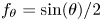$f_{\theta }=\sin (\theta )/2$, $\theta \in [0,{\rm \pi} ]$; and $f_{\phi ,\eta ,\psi }={\rm \pi} /2$, $\{\phi ,\eta ,\psi \} \in [0,2{\rm \pi} )$. The two random sets of spherical angles $\theta ^n$ and $\phi ^n$ cause the set of unit vectors, $\sigma _j^n$, to be uniformly distributed on a unit sphere. Imposing a divergence-free velocity ($\sigma _j^nd^n_j=0$ as verified in Smirnov et al. (Reference Smirnov, Shi and Celik2001)) together with the requirement that $d_j^n$ be uniformly distributed on a unit sphere leaves $d_j^n$ as a function of the dependent variables ($\theta ,\phi$) of $\sigma _j^n$ and the angle $\eta$ in the plane normal to $\sigma _j^n$. The random angles, radial lengths and defined intensities are wave modes that have been mapped to wave space from a pseudo-isotropic turbulence via the spatial Fourier transform. Note that the definition of $\hat {x}_i$ provides a means to slide through this pseudo-turbulence domain by a spatial coordinate that progresses at the inflow bulk speed, $U_0$, naturally accounting for bulk convection. The second argument of the $\max$ is due to Shur (M. L. Shur, private communication 2020). Definitions for $\kappa _e^{min}$, $f_\eta$, $f_{cut}$ and $k_e(x_i)$ match those given in Shur et al. (Reference Shur, Spalart, Strelets and Travin2014), where they were chosen to adjust the spectrum at each grid point on the inflow plane (eddy size and anisotropy) to accurately account for proximity to solid boundaries. Further, their approach of defining $a_{ij}$ through a Cholesky decomposition of the Reynolds stress, $R_{ij}$, is adopted.

An increase in the number of wave modes directly corresponds to the number of realizations of this pseudo-turbulence flow in addition to the recovery of the correct normalized energy spectra or, in physical space, the autocorrelation functions (Béchara Reference Béchara1994). However, as all implementations of this STG boundary condition will use a finite number of wave modes and a finite number of time steps, what remains to be seen is, with $N$ finite: (1) Does $\lim _{t\to \infty }\langle u_i'u_j'\rangle _t=R_{ij}$ and (2) does $\langle u_i'u_j'\rangle _t -\lim _{t\to \infty }[\langle u_i'u_j'\rangle _t]$ become acceptably small after a time $t$ that is otherwise sufficient to converge statistics within the interior of the simulation domain (e.g. a small number of domain flow-through times)? Is there a dependence of getting one but not the other? Issue (1) will be referred to as the bias (infinite-time realized Reynolds stress) and (2) as time convergence. This work aims to provide independent measures of each that will enable improvements to both.

3. Analysis tools

The analysis begins with the intent of recognizing the mathematical expressions that separate the bias and time convergence accuracy of a particular random number set for $N$ wave modes relative to the target covariance tensor of the velocity fluctuations:

(3.1)\begin{equation} \langle u_l'u_m'\rangle _t=a_{li}a_{mj}\langle v_i'v_j'\rangle _t, \end{equation}

where

(3.2a,b)\begin{equation} \langle [\,f] \rangle_t \equiv \frac{1}{t} \int^t_0 [\,f(t') ] \mathrm{d}t', \quad \langle [\,f] \rangle_{tz} \equiv \frac{1}{tz}\int^z_0\int^t_0 [\,f(t',z') ] \,\mathrm{d}t'\,\mathrm{d}z'. \end{equation}

Note from above that $a_{ij}$ provides a scaling to the velocity fluctuations, leaving $v_i$ to provide the instantaneous fluctuating direction, which follows from (3.1) and (2.1):

(3.3)\begin{equation} v'_i=2\sqrt{\tfrac{3}{2}}\sum_{n=1}^N\sqrt{q^n}\sigma^n_i \cos(\kappa^nd^n_l\hat{x}_l+\psi^n). \end{equation}

This also makes it clear that the covariance of the fluctuation tensor, $\langle v_i'v_j'\rangle _t$, should converge to $\delta _{ij}$, preferably within a time $t$ that is comparable to the time required for the Reynolds stresses to converge in an experiment. In this paper, we will refer to such an averaging time as a physical averaging time due to it realistically reflecting the nature of the turbulence, while inputs that require substantially longer averaging time to converge the stresses are considered non-physical averaging times.

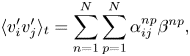
To better assess that, using (2.1), the covariance of the fluctuation tensor can be further decomposed into

(3.4)\begin{gather} \langle v_i'v_j'\rangle_t=\sum_{n=1}^N\sum_{p=1}^N\alpha_{ij}^{np}\beta^{np}, \end{gather}

(3.5a,b)\begin{gather}\alpha_{ij}^{np}\equiv 6\sqrt{q^nq^p}\sigma_i^n\sigma_j^p,\quad \beta^{np}\equiv\frac{1}{t}\int_0^t\cos(\gamma^nt'+\hat{\psi}^n({\boldsymbol{x}})) \cos(\gamma^pt'+\hat{\psi}^p({\boldsymbol{x}}))\,\mathrm{d}t', \end{gather}

(3.6a,b)\begin{gather}\gamma^n=\left.\frac{1}{t'}[\kappa^nd_i^n\hat{x}_i] \right|_{\boldsymbol{x}=\boldsymbol{0}}= -U_0d^n_1\max\left(2\kappa_{min},\frac{\kappa^n}{10}\right),\quad \left.\hat{\psi}^n=[\kappa^nd_i^n\hat{x}_i+\psi^n]\right|_{t'=0}. \end{gather}

Here, the fact that $\alpha _{ij}^{np}$ is independent of time has been exploited and the time integral has been propagated directly to $\beta ^{np}$, which captures all of the temporal variation of (3.4) and ultimately (3.1). Analytically integrating (3.5a,b) yields

(3.7)\begin{equation} \beta^{np}(t)=\left\{ \begin{array}{ll} \dfrac{\sin((\gamma^n+\gamma^p)t+\hat{\psi}^n+\hat{\psi}^p)}{2(\gamma^n+\gamma^p)t}+ \dfrac{\sin((\gamma^n-\gamma^p)t+\hat{\psi}^n-\hat{\psi}^p)}{2(\gamma^n-\gamma^p)t}, & n\neq p, \\ \dfrac{1}{2}+\dfrac{\sin(2(\gamma^nt+\hat{\psi}^n))}{4\gamma^nt}, & n = p. \end{array}\right\} \end{equation}

The value of this split is made more clear by considering the infinite-time limit of (3.7):

(3.8)\begin{equation} \lim_{t\rightarrow\infty}\beta^{np}=\tfrac{1}{2}\delta^{np}. \end{equation}

With these definitions, the previously stated two objectives (the bias and time convergence of this method) can now be analysed by independently inspecting $\sum _n\sum _p\alpha ^{np}\delta ^{np}/2=\sum _n\alpha ^{nn}/2$ (the infinite-time value of (3.4)) and $\beta ^{np}(t)$. From the former, it is clear that $\sigma _i^n$ influences the infinite-time bias with no influence from $d_i^n$. Conversely, the latter indicates that $d_i^n$, and specifically $d_1^n$, influences the temporal convergence with no influence from $\sigma _i^n$. This point is made more clear in subsequent sections but, for now, it is observed that the sine terms of (3.7) are bounded by 1 but the denominators beneath them are influenced by the size (for $n=p$) and closeness of magnitude (for $n \neq p$) of $\gamma ^n$, which is linear in $d_1^n$. The restriction that $d_i^n\sigma _i^n=0$ for each $n$ means that the prescriptions of $\alpha _{ij}^{np}$ and $\beta ^{np}$, while separable, are not completely independent of each other.

It is understood (Kraichnan Reference Kraichnan1970) that, as the number of realizations (or equivalently number of wave modes $N$) increases, the covariance of the fluctuation tensor in (3.1) converges to $\delta _{ij}$. Infinite or even very large $N$ is intractable for practical numerical simulations for the obvious reason of the cost of evaluating (2.1). In the sections that follow, $N$ will be treated as fixed to O $(500)$. It will be shown that this $N$ is large enough to allow acceptably low bias error and to allow time convergence of the STG fluctuations to mimic the physical time needed for time convergence of turbulence statistics within the interior of the simulation. This ensures that the unsteady inflow or scale-resolving interface does not artificially raise the number of time steps required by the simulation.

3.1. Error measurements

Below are measures of error for any given random number choice (through (3.5a,b)):

(3.9)\begin{gather} { e}^{{\alpha}}_{ij}=\alpha^{nn}_{ij}\tfrac{1}{2}-\delta_{ij}, \end{gather}

(3.10)\begin{gather}{ e}^{{R_b}}_{ij}=a_{il}a _{jm}{e} ^{{\alpha}}_{lm}, \end{gather}

(3.11)\begin{gather}{ e}_{{t}}^{np}=\langle \beta^{np}\rangle _t-\tfrac{1}{2}\delta^{np}, \end{gather}

(3.12)\begin{gather}{ e}^{{R_{t}}}_{ij}=a_{il}a_{jm}\langle v_jv_m\rangle _t-\langle u_i'u_j'\rangle _{t\to\infty}, \end{gather}

(3.13)\begin{gather}{ e}^{{R_t}}_{ij}\leqq \frac{24}{t}a_{il}a_{jm}\sum_{n=1}^N \sum_{p=1}^N \sigma^n_l\sigma^p_m\left\{ \begin{array}{ll} \dfrac{c q^n}{|\gamma^n|}, & n=p, \\ \dfrac{c\sqrt{q^nq^p}}{||\gamma^n|-|\gamma^p||}, & n\neq p, \end{array}\right\} \end{gather}

(3.14a,b)\begin{gather}{ e}^{{R}}_b={ e}^{{R_b}}_{ij}w _{jl}{e} ^{{R_b}}_{li},\quad { e}^{{R}}_t={ e}^{{R_t}}_{ij}w _{jl}{e} ^{{R_t}}_{li}. \end{gather}

These error measures will be explained in detail in the following two subsections.

3.2. Bias considerations

With a modest $N=O(500)$ spherically uniform random wave mode application, the bias in inflow spatio-temporal covariances has been observed to be up to 30 % off the target. The fluctuation bias error (3.9) depends upon a wave mode contraction of (3.5a,b), which exposes the dependence not only on $\sigma _i^n$ but also on the normalized energy of mode n, $q^n$, which is a function of position. Such an error measure neglects that the $a_{ij}$ is also a function of position and it further couples fluctuation errors. With the exception of $a_{11}$, the scaling is increasingly dependent on the accuracy of the other entries:

(3.15)\begin{equation} a_{ij}(x_l)=\left[\begin{array}{@{}ccc@{}} \sqrt{R_{11}(x_l)} & 0 & 0 \\ R_{21}(x_l)/a_{11} & \sqrt{R_{22}(x_l)-a_{21}^2} & 0 \\ R_{31}(x_l)/a_{11} & (R_{32}(x_l)-a_{21}a_{31})/a_{22} & \sqrt{R_{33}(x_l)-a_{31}^2-a_{32}^2} \end{array}\right]. \end{equation}

Take, for example, a non-zero fluctuation bias error in (3.9) and $R_{11}=R_{22}$. Then using (3.10) the percentage error on $R_{12}$ is

(3.16)\begin{equation} { e}^{{R_{b}}}_{12}/R_{21}= a_{11}a _{21}{e} ^{{\alpha}}_{11}/R_{21}+ a_{11}a _{22}{e} ^{{\alpha}}_{12}/R_{21}= { e}^{{\alpha}}_{11}+{ e}^{{\alpha}}_{12}\sqrt{(R_{11}/R_{21})^2-1}. \end{equation}

This is to say that the percentage difference of bias is proportional not only to the convergence of the isotropic fluctuation tensor but also to the ratio of the target stresses. Generally, the percentage error increases in growing row and column with any anisotropic stress and non-zero total fluctuation error. This propagation of error is directly accounted for in (3.10). However, to further compensate for this error amplification, the first equation in (3.14a,b) contracts the elements of the stress tensor error with a weight tensor, $w_{jl}$, which allows more weight to be given to stress components that are viewed as more important (e.g. shear stress) to accurately simulate the inflow, and to stress components that would otherwise accumulate more error.

With a precise measure of the bias error in hand, its inputs can be determined. As described in Shur et al. (Reference Shur, Spalart, Strelets and Travin2014), the target stresses are assumed known, potentially from an upstream RANS or other experiment. The normalized spectra are also assumed to be determined as a function of the inflow plane mesh resolution (which sets $\kappa _{max}$), the domain width (which sets $\kappa _{min}$), the wave mode spacing $\kappa ^n$ (with $\kappa ^n$ grown geometrically from $\kappa ^{min}$ to $\kappa ^{max}$ at a rate of ${\approx }1\,\%$), and the energy spectrum $E$ given as part of (2.1). This leaves only the four random angles needed to define $\sigma _j^n$, $d^n_j$ and $\psi ^n$. It is indeed these random number choices that will determine the bias of this procedure. Taking the first set of random angles could lead to an acceptable bias but, more than likely, will lead to a poor bias relative to what could be achieved by considering alternatives. Equations (3.14a,b) provide a means to evaluate the quality of a given random number set at any location on the inflow plane. That information can be used to find the worst location or can be averaged in space. Furthermore, the error can be studied over a variety of time intervals. Specific choices are discussed in § 4. Whatever the choice, by repeating this measurement for a large number of random number sets allows quick determination of the sets resulting in lowest bias, which is a key aspect of accurately matching the target inflow stress statistics.

4. Verification and results

As a test of the developments discussed above, a zero-pressure-gradient flow over a flat plate was considered. At the location of the inlet, the momentum thickness Reynolds number is $Re_\theta =1000$. The wall-normal spacing is typical of DNS with the first point located at $y^+=0.1$ growing geometrically at a rate of 1.05 until reaching approximately $y^+=10$, after which it is held at this spacing until $y=1.2 \delta _0$, where $\delta _0$ is the inflow boundary layer thickness. A structured spanwise spacing of $\varDelta _z^+=6$ is maintained throughout the inflow. The streamwise spacing influences the spectra (Shur et al. Reference Shur, Spalart, Strelets and Travin2014) and the time step and thus $\varDelta _x^+=10$ leads to a time step of $\varDelta _t=3\times 10^{-6}$, which corresponds to a non-dimensional time step of $\varDelta _t^+=0.2$. When studying the quality of the STG inflow on a flat plate, a domain length of $8{\rm \pi} \delta _0$ is adequate since the domain only needs to be long enough for the inflow to develop equilibrium stresses. Such a domain length has a flow-through time of $\varDelta _{ft}=8 {\rm \pi}\delta _0 / U_0$ or approximately 5000 time steps.

An example of the inflow Reynolds shear stress (the time and spanwise average of the covariance) obtained by applying (2.1) (with the first chosen set of random numbers) at the inflow is shown in figure 1(a). All target profiles are taken from a Spalart–Allmaras RANS simulation with the correction proposed by Coleman, Rumsey & Spalart (Reference Coleman, Rumsey and Spalart2018). The RANS simulation domain matched the DNS domain with an extension upstream to include a uniform flow stagnating upon a sharp leading edge from which the boundary layer develops. The RANS profiles were extracted at the DNS inflow location. In figure 1(a–d), the dash-dotted curve is a plot of the target shear stress profile. The dashed curve is the bias solution obtained by substituting (3.8) into (3.4) and further into (3.1), which displays how far off the target a first chosen random number set can be. The remaining curves of figure 1(a) display the span-time convergence at $t=1$, 2, 4 and 20 times $\varDelta _{ft}$. The random number set in figure 1(a) was not fabricated to illustrate poor bias; rather, it was one from a real simulation whose poor performance was finally attributed to this unexpectedly poor random number set after a substantial time integration. This random number set demonstrates the bias and temporal convergence of typically sampled sets.

Figure 1.

Reynolds shear stress $-R_{12}/u_{\tau }^2$ versus wall plus units: (a) typical random number set; (b) improved bias random number set; (c) $\sigma$-first sequential choice random number set; and (d) ‘intelligent’ design number set. Stress profile lines: dash-dotted, target; dashed, bias; solid, time convergence. Time level labelled with symbols: $\Box$, 1$\varDelta _{ft}$; $\diamond$, 2$\varDelta _{ft}$; $\triangleright$, 4$\varDelta _{ft}$; and $\triangleleft$, 20$\varDelta _{ft}$.

Applying only the bias improvement (e.g. keeping the $d_i^n$ vectors from those of figure 1(a), but considering a large collection of random number sets and choosing the one with low bias error according to the first equation in (3.14a,b)) results in figure 1(b). Applying $\sigma$-first sequential choosing is shown in figure 1(c). Note that the bias error is further improved in figure 1(c) relative to figure 1(b) due to the greater freedom of having two random numbers ($\theta ^n$ and $\phi ^n$) where figure 1(b) only had one ($\eta ^n$) due to $d_j^n$ being constrained to match figure 1(a). Figure 1(d) illustrates the results obtained with ‘intelligent design’. A different seed was used and thus the bias results are similar but not the same as figure 1(c) (showing the run-to-run variation in bias with a $\sigma$-first approach). Note the span-time average is also improved with figure 1(d) showing the least variation of the four cases.

The plots of figure 1 are not only time but also spanwise averaged, which, through the action of $\widehat {\psi ^n}$ can be seen in (3.7) to attenuate the time variation as the number of spanwise samples increases (average of sine is zero). Figure 1 is presented with spanwise averaging because it is the common way that researchers assess time convergence, exploiting the spatial homogeneity. However, a more clear view of the temporal convergence can be obtained by considering the normalized spanwise-varying stress fluctuation $f_{ij}=\langle u'^+_i u'^+_j \rangle _t (y,z) -\langle u'^+_i u'^+_j \rangle _{tz} (y)$, which decays as $\lim _{t\to \infty } f_{ij}=0$ without mixing in spatial averaging.

The variation of $f_{ij}$ with $\varDelta _{ft}$ is plotted two ways in figure 2 for each of the four cases considered in figure 1. The dashed lines show $f_{ij}^{max}=\max _y(\max _z(\,f_{ij}))$, which can be thought of as the largest local stress deviation from its spanwise average for a given interval's time average (e.g. error of the poorest converged stress across the entire inflow plane). The solid line shows $f_{ij}^{rmy}=\max _y(\,f_{ij}^{rms})$, which can be thought of as the least time-converged r.m.s. variation of $f_{ij}$.

Figure 2.

Time convergence of spanwise variation of stress fluctuations as a function of flow-through times: $f_{12}^{max}$ (dashed); $f_{12}^{rmy}$ (solid). Symbols: $+$, figure 1(a); $\triangleright$, figure 1(b); $\triangleleft$, figure 1(c); $\times$, figure 1(d); $\cdots \cdots$, DNS channel.

As this is a somewhat non-traditional quantity, the channel flow DNS database of (Graham et al. Reference Graham, Kanov, Yang, Lee, Malaya, Lalescu, Burns, Eyink, Szalay and Moser2016) was used to assess the expected level of $f_{12}^{max}$ and $f_{12}^{rmy}$ after one channel flow-through time. This channel flow database was chosen over flat-plate data because of the lack of inflow boundary condition assumptions. The $Re_\tau$ for both cases are similar – this paper's flat plate ranges from $Re_{\tau }=600\text {--}1000$ while the channel $Re_{\tau }=1000$. Mining the entire time-continuous segment of the database (one channel flow-through time) at five wall-normal locations and 10 streamwise locations yielded values of $f_{12}^{max}\approx 0.7$ and $f_{12}^{rmy}\approx 0.2$, which are added to figure 2 as dotted lines. Comparing the dashed curves, none of the curves meets the channel value of $f_{12}^{max}$ at $2 \varDelta _{ft}$ though most have by $4 \varDelta _{ft}$. Likewise, comparing the solid curves, all four cases are close to $f_{12}^{rmy}$ of the channel after $2 \varDelta _{ft}$ but only the ‘intelligent design’ case exhibits the expected asymptotic $1/t$ convergence after $4\varDelta _{ft}$ as it also did for $f_{12}^{max}$. It must be noted that the Reynolds number and flow (channel versus boundary layer) differences likely render the dotted lines as rough targets/guidelines for temporal convergence measures.

Though not shown here, the choice of $\psi ^n$ influences early-time convergence through the numerator of (3.7), but, as most scale-resolving simulations integrate over multiple $\varDelta _{ft}$, the improved convergence in the $t \geq 4 \varDelta _{ft}$ range from ‘intelligent design’ is significant. Note that figure 2 shows that the time convergence of the case in figure 1(c) is as good as or better than the cases in figure 1(a) and figure 1(b). This contradicts the visual results in figure 1 confirming the muddled view of time convergence introduced by spanwise averaging in figure 1.

While the prediction of the shear stress at the inflow is the most important stress, the normal stresses are also important in some applications. Figure 3 shows that the mode set that created figure 1(d) (‘intelligent design’) resulted in excellent biases for the normal stresses as well. Note that all three target stresses were set to isotropic values consistent with information available from a one- or two-equation RANS closure. To achieve this result, in (3.14a,b), $w_{12}=w_{21}=25$, $w_{22}=5$ and all other $w_{ij}=1$. Equal weights for all components yielded relatively larger bias error (not shown) in $R_{12}$ as noted in (3.16).

Figure 3.

Normal Reynolds stress profile with ‘intelligent design’ random number set at $2\varDelta _{ft}$. Symbols: - - - -, $R_{iso}$; $\circ$, $R_{11}$; $+$, $R_{22}$; $\times$, $R_{33}$.

Direct numerical simulations with two different random number sets were performed, and the evolution of the wall coefficient of friction $C_f$ is shown in figure 4. The high-bias random number simulation requires a substantially longer development length to reach the 5 % margin from Smits et al. (Reference Smits, Matheson and Joubert1983) correlation, which at this Reynolds number is in good agreement with Coles's (Reference Coles1962) experiment and Jimenez et al.'s (Reference Jimenez, Hoyas, Simens and Mizuno2010) DNS. The low-bias inflow reaches the 5 % margin within two to three boundary layer thicknesses as opposed to six for the high bias. Both eventually come to better agreement in eight and 10 boundary layer thicknesses, respectively. Better agreement in the early region offers significant advantage when applied to flows with pressure gradients whose development is not as forgiving as the zero-pressure-gradient cases presented here.

Figure 4.

Coefficient of friction versus development length for high-bias (dashed) and low-bias (solid) inflow; Smits, Matheson & Joubert (Reference Smits, Matheson and Joubert1983) correlation (dash-dotted) with 5 % variation (dotted); Coles (Reference Coles1962) experiment, $\Box$; and Jimenez et al. (Reference Jimenez, Hoyas, Simens and Mizuno2010) DNS, $\circ$.

It is important to mention that the spike in wall shear immediately downstream of the inflow is to be expected with this STG method (Shur et al. Reference Shur, Spalart, Strelets and Travin2014), and is caused by the near-wall synthetic turbulence developing the correct physics (e.g. wall streaks). As a consequence, this spike is larger with DNS (see also the simulations of Spalart et al. (Reference Spalart, Belyaev, Garbaruk, Shur, Strelets and Travin2017)) than with other methods that do not fully resolve the near-wall turbulence, such as the hybrid RANS/LES model used in Shur et al. (Reference Shur, Spalart, Strelets and Travin2014) and figure 6. The shear stress profiles shown in figure 5 illustrate the same delayed convergence of the high-bias inflow relative to the low-bias inflow. At $3\delta _0$ downstream the high-bias stress profile has a substantial bulge in the range of $0.1 < y/\delta _0 < 0.6$, which decreases in both magnitude and range, $0.25 < y/\delta _0 < 0.6$ by $5\delta _0$, and is virtually eliminated by $10\delta _0$.

Figure 5.

Reynolds shear stress profiles for high (dash) and low (solid) inflow bias at 3 ($\circ$), 5 ($\Box$) and 10 ($\triangle$) boundary layer thicknesses downstream of inflow.

As additional verification of the correctness of the implementation of Shur et al.'s (Reference Shur, Spalart, Strelets and Travin2014) method, we repeat one simulation performed therein – a wall-modelled LES of fully developed turbulent flow in a channel. In order to allow direct comparisons to the original results of the method, the problem set-up matched those described in Shur et al. (Reference Shur, Spalart, Strelets and Travin2014). The Reynolds number based on the half-height is $Re_\tau =400$, the grid has spacing ${\rm \Delta} x^+=40$, ${\rm \Delta} z^+=20$, ${\rm \Delta} y^+_{min}=0.8$ and ${\rm \Delta} y_{max}=0.04H$, where $H$ is the channel height. The turbulence model used was IDDES (improved delayed detached-eddy simulation) (Shur et al. Reference Shur, Spalart, Strelets and Travin2008) based on the Spalart–Allmaras RANS closure (Spalart & Allmaras Reference Spalart and Allmaras1994). Figure 6 shows that, for this channel flow, similarly to the flat-plate boundary layer, with the STG inflow boundary condition the skin friction is recovered within $3\delta$ ($\delta =H/2$) and the Reynolds shear stress agrees well with the solution obtained with periodic boundary conditions at $6\delta$ as shown in figure 7. These results are consistent with the ones obtained by Shur et al. (Reference Shur, Spalart, Strelets and Travin2014) for the IDDES-SST (shear stress transport) $k$–$\omega$ model.

Figure 6.

Coefficient of friction as a function of development length for a wall-modelled LES of a channel utilizing STG (solid line) compared to periodic boundary conditions ($\circ$).

Figure 7.

Reynolds shear stress profile six boundary layer thicknesses downstream of STG inflow (solid line) compared to results obtained with periodic boundary conditions ($\circ$), both using wall-modelled LES.

It is important to highlight that the analysis of the errors and the choosing of the random variables that are the focus of this paper are completely independent of the specific flow problem. Of course, the target mean velocity and stress profiles will change; however, the process of minimizing bias and obtaining adequate time convergence of the statistics does not (with the exception of the selection of the weights in (3.14a,b), which should be tailored to prioritize the most important stress components).