1. Introduction
Flapping flight of natural flyers exhibits remarkable flight performance in the low-Reynolds-number regime, allowing them to adapt to a variety of flight environments (Shyy et al. Reference Shyy, Kang, Chirarattananon, Ravi and Liu2016; Liu et al. Reference Liu, Wang and Liu2024b ). Among various flapping foil creatures, those with tandem foils, such as dragonflies, which are believed to be one of the most successful aerial predators on Earth, exhibit superior flight performance compared with other natural fliers (Combes et al. Reference Combes, Rundle, Iwasaki and Crall2012). Compared with the configuration of a single foil, the most significant difference is that there exist foil–foil interactions in the tandem foils configuration, which would remarkably alter the aerodynamics, especially for the hind foil, and it has been revealed that the complex vortex dynamics induced by the foil–foil interactions can improve the aerodynamic performance within specific parameter spaces (Lian et al. Reference Lian, Broering, Hord and Prater2014; Noda et al. Reference Noda, Liu, Hefler, Shyy and Qiu2023). For example, a drag reduction effect for the hind foil (also termed as boosting effect) can be observed, resulting from the fact that it captures the vortices shed from the fore foil (Gong, Jia & Xi Reference Gong, Jia and Xi2015; Lua et al. Reference Lua, Lu, Zhang, Lim and Yeo2016; Joshi & Mysa Reference Joshi and Mysa2021; Wang et al. Reference Wang, Ng, Teo, Lua and Bao2021; Ormonde et al. Reference Ormonde, Kurt, Mivehchi and Moored2024). In addition, the effect of the flapping styles (Wang et al. Reference Wang, Ng, Teo, Lua and Bao2021; Liu et al. Reference Liu, Li, Xiang, Li and Tu2024a ), phase difference (Lua et al. Reference Lua, Lu, Zhang, Lim and Yeo2016; Lagopoulos, Weymouth & Ganapathisubramani Reference Lagopoulos, Weymouth and Ganapathisubramani2020) and flexibility (Cong, Teng & Cheng Reference Cong, Teng and Cheng2020; Noda et al. Reference Noda, Liu, Hefler, Shyy and Qiu2023) have also been taken into account. In this study, inspired by near-wall forward flight in biological systems (Hainsworth Reference Hainsworth1988; Park & Choi Reference Park and Choi2010), we focus on the aerodynamics of two tandem foils flapping near a boundary layer (BL) developed in a wall-bounded shear flow. Since this BL must coexist with a ground (or referred to as the ‘wall’), we first review the studies on the ground effect for a single or multiple flapping foils, followed by a discussion on the evolution of the wake flow, which governs the aerodynamic forces.
The ground effect has been well studied in the case of a single flapping foil in both hovering (Gao & Lu Reference Gao and Lu2008; Lu et al. Reference Lu, Lua, Lim and Yeo2014; Wu et al. Reference Wu, Liu, Yang and Zhao2015) and forward flight (Quinn et al. Reference Quinn, Moored, Dewey and Smits2014; Wu et al. Reference Wu, Shu, Zhao and Yan2014; Han et al. Reference Han, Zhong, Mivehchi, Quinn and Moored2024) modes. Comparatively speaking, this effect has been less discussed in the case of tandem foils. In 2017, Srinidhi & Vengadesan (Reference Srinidhi and Vengadesan2017) studied the ground effect on tandem wings flapping in an inclined hovering mode, and complex wing–wing interactions are observed; it is further found that the maximum lift can be achieved via the in-phase motion of tandem wings and that counter stroking increases the stability of the wings in hovering. For the ground effect in the forward flight mode, Yang et al. (Reference Yang, He, Mo and Wang2021) studied the energy extraction performance, and an increase in the energy extraction efficiency is observed with the presence of the ground effect; while a significant drop occurs if there is a 180
 $^{\circ }$
phase difference between the fore and hind hydrofoils, despite an increase in lift. Duan et al. (Reference Duan, Wang, Zhou, Jia and Zhong2024) preformed a physical and data-driven study of the ground effect on the propulsive performance of tandem flapping wings. The authors found that a smaller phase difference between the fore and hind wings can lead to a higher thrust, while the boosting effect induced by the ground on the hind wing will be diminished. It is worth noting that in studies on the ground effect (hereafter termed as ‘pure ground effect’ for a clear distinction) in the forward flight mode, the ground is typically modelled as a kinematically matched moving wall to eliminate near-wall shear in the flow field (Moryossef & Levy Reference Moryossef and Levy2004; Wu et al. Reference Wu, Shu, Zhao and Yan2014; Duan et al. Reference Duan, Wang, Zhou, Jia and Zhong2024). In other words, these studies intentionally exclude the influence of viscous BL development.
The evolutionary behaviours of wake flow depend on the vortex dynamics therein, which has been studied a lot for both the case of a single foil (Dewey, Carriou & Smits Reference Dewey, Carriou and Smits2012; Andersen et al. Reference Andersen, Bohr, Schnipper and Walther2017; Jones, Kanso & Luhar Reference Jones, Kanso and Luhar2024) and that of tandem foils (Kumar & Hu Reference Kumar and Hu2011; Lagopoulos et al. Reference Lagopoulos, Weymouth and Ganapathisubramani2020). The vortex dynamics in the wake is driven by the periodic flapping of the foil(s). It is then natural to imagine that the evolution of the wake flow will evolve synchronously with the same period as the flapping cycle; while aperiodic evolution of the wake flow, thereby of the aerodynamic force, has been observed, under specific parameter conditions. Lewin & Haj-Hariri (Reference Lewin and Haj-Hariri2003) studied the effect of the reduce frequency
 $\kappa$
and that of the Strouhal number
 $St$
on the vortex dynamics of a single plunging aerofoil at a Reynolds number of
 ${\textit{Re}}=500$
, and it is found that the aperiodic evolution occurs when
 $\kappa \geqslant 6$
and
 $ St \geqslant 0.35$
. Building on this result, subsequent studies have concluded that the maximum non-dimensional plunge velocity
 $ \kappa H_m/c$
(
 $H_m$
indicates the plunging amplitude and
 $c$
the chord length, see § 2) is a key parameter in modulating the evolution of the wake flow (Ashraf, Young & Lai Reference Ashraf, Young and Lai2012; Khalid et al. Reference Khalid, Akhtar, Dong, Ahsan, Jiang and Wu2018). Bose & Sarkar (Reference Bose and Sarkar2018) pointed that the evolution of the leading edge vortex (LEV) is the key factor in the transition from the periodic to chaotic vortex evolution, where the irregular shedding time of the LEV at high plunge velocities drives this transition. Later, Majumdar et al. (Reference Majumdar, Bose and Sarkar2022) evaluated the circulation of the LEV quantitatively, revealing that lower intensity LEVs correspond to periodic and quasi-periodic flows, whereas higher intensity ones are associated with chaotic flows. In addition, the maximum effective angle of attack and the leading-edge amplitude-based Strouhal number are proved to be able to effectively capture the physical effect of the parametric variations on the wake dynamics. Most recently, the chaotic evolution behaviours in the wake flow of a flexible flapping foil were investigated by Shah et al. (Reference Shah, Majumdar, Bose and Sarkar2024), which, for a rigid foil, can only be achieved via a quasi-periodic-intermittency route under high plunge velocities (Badrinath, Bose & Sarkar Reference Badrinath, Bose and Sarkar2017). Unlike the case for a rigid foil, as the flexibility gradually increases, the foil will regulate aperiodic into periodic motion by generating various wake patterns. When the flexibility exceeds an optimal level, the aperiodic evolution behaviour re-emerges, eventually leading to chaotic evolution behaviours under extremely high flexibility conditions. In addition, it is worth mentioning that Moriche et al. (Reference Moriche, Flores and García-Villalba2016, Reference Moriche, Flores and García-Villalba2017) reported explicitly a phenomenon of period doubling in the evolution of the wake flow; however, the authors did not analyse the associated nonlinear dynamics. Meanwhile, it should be noted that the evolutionary dynamics already reviewed here are limited to the configuration of a single foil flapping in the free flight scenario, without the presence of a ground or a wall-bounded shear flow.
The effect of the wall-bounded shear flow is generally considered in the configuration of one or multiple cylinders, where the aforementioned period change of the system evolution can be also observed (He, Wang & Pan Reference He, Wang and Pan2013; Rao et al. Reference Rao, Thompson, Leweke and Hourigan2013; Shaafi & Vengadesan Reference Shaafi and Vengadesan2014). Most recently in 2025, this effect (termed as ‘near-wall effect’ therein) has also been considered on the vortex dynamics in the flow around a rectangular cylinder, and it is found that the gap ratio between the rectangular cylinder and the wall, as well as the cylinder’s aspect ratio, significantly modulate the vortex dynamics and turbulence transport in the wake flow (Li et al. Reference Li, Wang, Qiu, Zhou, Fu and Liu2025a , Reference Li, Wang, Qiu, Zhou, Fu and Liub ). When it comes to the flapping foil, this effect has only been explored for the configuration of a single foil by Lin et al. (Reference Lin, Jia, Wang and Zhong2024), where significant modulations are observed on both aerodynamic forces and the flow structures. Comparing with the aforementioned pure ground effect, the aerodynamic forces exhibit greater fluctuations and a more complex vortex dynamics is seen, with the presence of the secondary vortices and the sheltering effect of the BL. However, it should be pointed out that, for this configuration of a single foil, no aperiodic evolution is observed in the considered parameter space (same as the present study, see § 3.4). As for the aerodynamic forces and wake vortex dynamics of tandem foils, to our best knowledge, the effect of the wall-bounded shear flow has not been documented, so far.
In this study, we aim to investigate how the presence of a viscous BL developing along a stationary no-slip wall modulates the unsteady aerodynamics and wake dynamics of two tandem flapping foils. Unlike the widely studied pure ground effect, in which the wall is modelled as a kinematically matched moving boundary to eliminate near-wall shear and thus to exclude BL development intentionally (Moryossef & Levy Reference Moryossef and Levy2004; Wu et al. Reference Wu, Shu, Zhao and Yan2014; Duan et al. Reference Duan, Wang, Zhou, Jia and Zhong2024), the present configuration introduces a viscous wall-bounded shear layer that interacts dynamically with the vortical structures shed by the tandem foils, leading to a fundamentally different coupling mechanism. Meanwhile, we emphasise that the present work does not aim to isolate a ‘pure BL effect’ in the classical sense. Instead, it examines how the presence of a wall-bounded shear layer modifies the unsteady aerodynamics and wake dynamics of tandem flapping foils. In this configuration, the viscous BL plays a central role in shaping the flow field, which constitutes the most prominent distinction from the mechanism underlying the pure ground effect. For brevity, we refer to the influence of this wall-bounded shear layer as the ‘BL effect’ throughout this study.
The rest of the paper is organised as follows. In § 2, we describe the formulation of problem and the numerical method. Then, in § 3, we present and discuss the results on aerodynamic forces and flow patterns, where the vortex dynamics are explored through Lagrangian coherent structures revealed by the finite-time Lyapunov exponent, modal analysis for frequency response and bifurcation analysis. Finally, concluding remarks are summarised in § 4.
2. Modelling
As illustrated in figure 1, this study investigates two tandem foils flapping in the forward flight mode, interacting with a BL along a fixed no-slip flat wall. The configuration is two-dimensional, with the flow assumed to have infinite span. The foils therefore undergo prescribed plunging and pitching motions without spanwise variation, and three-dimensional effects such as tip vortices are neglected. Both foils are modelled as two identical NACA0012 aerofoils with a chord length of
 $c$
, and the equations governing the plunging and pitching motions of the fore and hind foils are as follows:
 \begin{align} H_f(t) & = H_{m} \cos {\left (2 \pi t /T\right )}+ H_{0}, \end{align}
 \begin{align} \alpha _f (t) & =-\alpha _{m} \sin {\left (2 \pi t /T\right )}+\alpha _{0}, \end{align}
 \begin{align} H_h(t) & = H_{m} \cos {\left (2 \pi t /T \right )}+ H_{0}, \end{align}
 \begin{align} \alpha _h (t) & = -\alpha _{m} \sin {\left (2 \pi t /T \right )}+\alpha _{0}. \end{align}
(a) Computational domain and boundary conditions for the present tandem flapping foils configuration. (b) Two sets of meshes used in the immersed boundary-lattice Boltzmann method: a fixed Eulerian mesh for the flow field and a dynamic Lagrangian mesh for the moving solid boundaries immersed in the fluid. (c) Schematic of the tandem flapping foils interacting with the BL (shown in grey) at a stationary, flat and no-slip wall. This schematic corresponds to an enlarged view of region framed by the red dashed frame in panel (a). The locations and orientations of the foils during the downstroke and upstroke phases are denoted by black solid and red dashed lines, respectively. Please note that these schematics are not to scale for a clear view.

In these equations,
 $T$
represents the period of the plunging and pitching motion, and we consider no phase difference between plunging and pitching motions for both foils. Here,
 $H_f(t)$
and
 $H_h(t)$
denote the distances from the pitching axes of the fore and hind foils to the wall, respectively,
 $H_0$
is the mean distance, and
 $H_m$
indicates the amplitude of the plunging motion. Additionally,
 $\alpha _f(t)$
and
 $\alpha _h(t)$
measure the angles of attack, with
 $\alpha _0$
and
 $\alpha _m$
being the mean attack angle and the amplitude of the pitching, respectively. The flapping kinematics adopted here follow Wu et al. (Reference Wu, Shu, Zhao and Yan2014) and Lin et al. (Reference Lin, Jia, Wang and Zhong2024), where, however, only a single foil is studied. This selection enables a direct comparison among the pure ground effect condition, the single-foil BL configuration and the present tandem foils case. Using identical kinematics allows all observed differences to be attributed to the interactions between the tandem foils and the wall-bounded shear (i.e. the BL effect) rather than motion parameters. As indicated by (2.1)–(2.4), the fore and hind foils perform synchronous motions, indicating no phase difference between them, to highlight the effect of the BL. In addition, it should be pointed out that, throughout this manuscript, the subscripts ‘
 $f$
’ and ‘
 $h$
’ represent quantities and parameters associated with the fore foil and the hind foil, respectively. Fluid flow past the tandem foils is governed by the incompressible Navier–Stokes equations
 \begin{align} \boldsymbol{\nabla \boldsymbol{\cdot }u} & = 0, \end{align}
 \begin{align} \frac {\partial \boldsymbol{u}}{\partial t} + \boldsymbol{u}\boldsymbol{\cdot }\boldsymbol{\nabla u} & = -\frac {1}{\rho }\boldsymbol{\nabla } p + \nu {\nabla ^2 u} . \end{align}
Here,
 $\boldsymbol{u}$
represents the fluid velocity,
 $\rho$
is the mass density,
 $p$
denotes the hydrostatic pressure and
 $\nu$
is the kinematic viscosity.
Under the given flapping motions, the aerodynamics of the tandem foils can be characterised by the Strouhal number and the Reynolds number. The Strouhal number, defined as
 $St = 2H_{m}/(U_{\infty }T)$
, characterises the periodic unsteadiness of the flow. Reynolds number is defined as
 ${\textit{Re}}=U_{\infty }c/\nu$
, based on the free stream velocity
 $U_{\infty }$
and the chord length
 $c$
, and it is employed as one of the control parameters to measure the effect of the BL in this work. In the subsequent analysis,
 $St$
is kept constant and the effect of
 ${\textit{Re}}$
on the aerodynamic forces acting on the tandem flapping foils, as well as on the downstream flow patterns, is examined. The aerodynamic force is further decomposed into a lift (
 $F_l$
) acting in the
 $+y$
direction and a drag (
 $F_d$
) acting in the
 $+x$
direction. As a result, the lift and drag coefficients, along with their mean values over one flapping period of
 $T$
, are defined as follows:
 \begin{eqnarray} C_l=\frac {2F_l}{\rho U_{\infty }^{2} c} \, , \quad C_d=\frac {2F_d}{\rho U_{\infty }^{2} c}\, , \quad \overline {C}_l =\frac {1}{T} \int _0^T C_l\, \textrm{d}t \, , \quad \overline {C}_d = \frac {1}{T} \int _0^T C_d\, {\textrm{d}}t . \end{eqnarray}
On the solid walls, the no-slip condition is imposed, to both the stationary bottom wall and the foils’ surfaces. Regarding the boundary conditions on the computational domain, they will be specified later at the beginning of § 3.
2.1. Numerical method and validations
In this study, a custom-made code implementing the lattice Boltzmann method (LBM) is developed to solve the system via direct numerical simulations, owing to the nonlinear nature of the fluid flow around the foils and in the wake (see (2.5)–(2.6)). LBM has gained significant popularity in recent years due to its high computational efficiency and numerical stability (Guo & Shu Reference Guo and Shu2013). In this method, the fluid flow is represented by a density distribution function, which is encoded by the lattice Bhatnagar–Gross–Krook (LBGK) model in this study, and the LBGK model is implemented through the D2Q9 model (Qian, d’Humières & Lallemand Reference Qian, d’Humières and Lallemand1992), based on an orthogonal Eulerian grid (figure 1 b). Dynamic motions of the tandem flapping foils are described by using the immersed boundary method (IBM), which effectively captures flow fields with complex and/or moving boundaries (Peskin Reference Peskin1972). Here, we employ a non-iterative IBM, introduced by Tao et al. (Reference Tao, He, Chen, Chen, Yang and Wu2019, Reference Tao, Wang, He, Chen and Luo2022), which eliminates the need to invert large matrices as required in traditional approaches (Wu & Shu Reference Wu and Shu2009), significantly enhancing computational efficiency, and meanwhile ensuring the no-slip boundary condition at the solid surface. Consequently, we embed the non-iterative IBM into the LBM to model the boundary conditions at the moving solid foils in the flow field, resulting in the so-called non-iterative immersed boundary-lattice Boltzmann method (IB-LBM). This method uses two sets of meshes: a Lagrangian mesh for the foils and an Eulerian mesh for the flow field, as shown in figure 1(b). Additional details about this non-iterative IB-LBM can be found from Lin et al. (Reference Lin, Jia, Wang and Zhong2024).
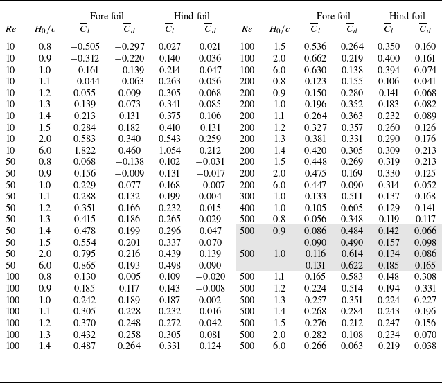
Now, we present the validation of the custom-made code implementing the non-iterative IB-LBM, by simulating the tandem flapping foils cases reported in the literature. In figure 2, we compare the drag coefficients of the fore and hind foils over a complete flapping cycle from the present calculations with those reported by Wu et al. (Reference Wu, Li, Chen and Zhang2022) for a two-dimensional tandem flapping-fixed aerofoil configuration. Good agreements are observed in the drag coefficient
 $C_d$
for both foils, and it is worth noting that the obtained lift coefficient
 $C_l$
and the flow fields (not shown here) are also well consistent with those reported in the literature, which we choose not to show for brevity. Therefore, we conclude that the present custom-made code is capable of accurately studying the aerodynamics of the tandem foils in question.
Validations of the present numerical method and the custom-made code. Comparisons of the present calculations with the reported data for the tandem flapping-fixed aerofoil configuration of Wu et al. (Reference Wu, Li, Chen and Zhang2022) for the drag coefficients of (a) the fore foil and (b) the hind fixed foil during one flapping cycle, where the distance between two foils is
 $3c$
in the flow direction, with a zero attack angle for the hind fixed foil. Curve conventions are given in panel (a) for both panels.

3. Results and discussions
In this section, we present and discuss the results. Prior to talking about the obtained results, we discuss the parameter settings used in this study.
For both foils in this tandem configuration, the pitching axis is located at the midpoint of the chord length, and the amplitudes of plunging and pitching are fixed to be
 $H_{m}=0.4c$
and
 $\alpha _{m}=\pi /4$
, respectively; and the mean attack angle is set to be
 $\alpha _{0}=0$
. As for these flapping kinematics parameter choices, we clarify here further that they follow directly from the frameworks of Wu et al. (Reference Wu, Shu, Zhao and Yan2014) and Lin et al. (Reference Lin, Jia, Wang and Zhong2024), ensuring a controlled progression from the pure ground effect condition to the single-foil BL case and, finally, to the tandem foils configuration studied here. Each stage introduces only one additional physical factor, thereby isolating the specific influence of the tandem foils and BL interaction. In all simulations, the Strouhal number is fixed at
 $St=0.3$
, which lies within the typical range of
 $0.2 {-} 0.4$
observed in natural flyers (Taylor, Nudds & Thomas Reference Taylor, Nudds and Thomas2003), and a constant
 $St$
also isolates the effects of
 $H_0/c$
and
 ${\textit{Re}}$
on the aerodynamic forces and vortex dynamics, without introducing additional variations arising from changes in flapping frequency or amplitude. First,
 ${\textit{Re}}$
varies within the range of
 $10 \leqslant Re \leqslant 500$
and it is later extended to 1000 for the discussions on the dynamical behaviours of the system in § 3.4. The range of Reynolds number (
 $\mathcal{O}(10) {-} \mathcal{O}(10^3)$
) under consideration encompasses laminar to early-transitional regimes typical of natural small-scale flyers (Liu et al. Reference Liu, Wang and Liu2024b
), and provides a wide variation of BL thickness and vorticity diffusion to be further discussed by the end of § 3.2. For each
 ${\textit{Re}}$
, the degree of interaction between the tandem foils and the BL is adjusted by varying the mean position
 $H_{0}$
, within the range of
 $0.8 \leqslant H_{0}/c \leqslant 6.0$
, where the lower limit avoids physical overlap with the wall while maintaining strong wall interaction and the upper limit ensures a nearly wall-independent free flight scenario.
The computational domain is a rectangle of the size
 $60c \times 30c$
and the locations of the foils are illustrated in figure 1(a,c). The fore foil is positioned
 $20c$
from the leading edge of the bottom no-slip wall to allow for a sufficient development of the BL along the wall. The hind foil is positioned
 $1.5c$
downstream from the fore foil in the
 $x$
direction. This separation distance can induce an essential coupling between the two foils, meanwhile avoiding the interference (Pan et al. Reference Pan, Deng, Shao and Liu2016). As for the boundary conditions, no-slip condition for the fluid velocity is imposed on solid surfaces, as stated earlier after (2.7). At the top of the computing domain, the free shear condition (
 $\partial u / \partial y =0$
and
 $v=0$
) is applied to prevent the outflow therein, and an outlet condition (
 $\partial u / \partial x =0$
and
 $\partial v / \partial x =0$
) is imposed for the right boundary as a velocity outlet to enable the velocity to be convected freely out of the domain. At the inlet of the domain, a free stream velocity
 $U_{\infty }$
is imposed. The velocity field is initialised as
 $u=U_{\infty }$
and
 $v = 0$
for each simulation, and after a sufficiently long time, the system is expected to evolve in a periodic way. The evolutionary behaviour of the system will be the central topic of the subsequent discussions. Another important aspect to clarify is the grid independence. As shown in figure 3, we present
 $C_d$
obtained from three different meshes with
 $\Delta x / c= 1/100$
,
 $\Delta x / c= 1/200$
and
 $\Delta x / c= 1/240$
for the case of
 ${\textit{Re}} = 200$
and
 $H_0/c=1.5$
in the tandem foils configuration under consideration. It is observed that the results of the coarse mesh (
 $\Delta x / c= 1/100$
) deviate slightly from those of the medium and the fine meshes (
 $\Delta x / c= 1/200$
and
 $\Delta x / c= 1/240$
), and the medium and the fine meshes provide almost identical results. Similar results can be observed in
 $C_l$
of both foils and these results are omitted for brevity. Therefore, the medium mesh size
 $\Delta x / c= 1/200$
is selected for the simulations, as it provides a good balance between the numerical accuracy and the computational efficiency. Parameter settings and averaged aerodynamic force coefficients are summarised in Appendix A.
Validations of the present numerical mesh. Temporal evolution of the fore foil and hind foil drag coefficients over one flapping period for different mesh spacing of the lattice at
 ${\textit{Re}}=200, \, H_0/c=1.5$
. Drag coefficients for (a) fore foil and (b) hind foil are shown. Curve colour conventions are given in panel (a) for both panels.

In the subsequent discussions, we will first examine the aerodynamic forces and flow patterns resulting from the interactions between the tandem foil and the BL at the wall, highlighting the difference compared with the case of a single foil as reported by Lin et al. (Reference Lin, Jia, Wang and Zhong2024) and the pure ground effect condition as noted by Duan et al. (Reference Duan, Wang, Zhou, Jia and Zhong2024). A detailed discussion is first conducted on the behaviours of the instantaneous and mean aerodynamic forces, where a temporal evolution period doubling of the forces is observed. Next, this period doubling phenomenon is thoroughly discussed by analysing the wake coherent structures using the finite-time Lyapunov exponent (FTLE) field and the dynamic mode decomposition (DMD) technique. In the last subsection, from the point of view of a dynamical system, nonlinear time series analysis is performed to study the bifurcation nature of the period variations of the system’s evolution.
3.1. Aerodynamic forces modulated by the boundary layer
In this subsection, we first compare the pure ground condition with the BL case. Then, we discuss the temporal evolution of the aerodynamic forces, followed by an analysis of the average lift and drag over one flapping cycle.
To highlight the influence of the BL along the wall, figure 4 presents the temporal evolution of the lift coefficient of the hind foil (as a representative force coefficient) over one flapping cycle, together with the near-wall vorticity fields at the beginning of each cycle, for tandem foils interacting with a viscous BL and for those operating under the pure ground effect, at
 $H_0/c = 1.0$
and
 ${\textit{Re}} = 100$
. It is evident that the case with the BL (red curve in figure 4
a) exhibits markedly stronger force oscillations compared with that under the pure ground effect (blue curve in figure 4
a). This observation is consistent with the behaviour reported for a single flapping foil by Lin et al. (Reference Lin, Jia, Wang and Zhong2024) (see figure 4 therein). These results demonstrate that the presence of the BL introduces additional viscous and vortical coupling mechanisms absent in pure ground effect flows. As shown in figure 4(b,c), clear distinctions can be observed in the vortex dynamics in the wake.
Evolution of the lift coefficient and near-wall vorticity fields for tandem foils interacting with a viscous BL and under the pure ground effect, at
 $H_0/c = 1.0$
and
 ${\textit{Re}} = 100$
. (a) Lift coefficient
 $C_l$
of the hind foil. Normalised vorticity fields (
 $\omega c / U_\infty$
) at the beginning of the flapping cycle for (b) the pure ground effect case and (c) the tandem foils–BL interaction case.

Now, we discuss the temporal evolution of the aerodynamic forces in the presence of the BL. We present the results of two cases with different values of
 $H_0/c$
, but both at
 ${\textit{Re}} = 100$
, for comparisons in figure 5. Additionally, the results for the configuration of a single flapping foil, obtained with the same parameters, are included as well to emphasise the interactions between the two tandem foils.
Comparisons of
 $C_l$
and
 $C_d$
between the tandem foils configuration and the single foil configuration. Temporal evolution of the lift and drag coefficients over one flapping cycle after the system reaches the statistically steady state for
 ${\textit{Re}}=100$
,
 $H_0/c=0.8$
and
 $6.0$
. The lift coefficient
 $C_l$
is shown for (a) fore foil and (b) hind foil; the drag coefficient
 $C_d$
is shown for (c) fore foil and (d) hind foil. Dashed lines in each panel correspond to
 $C_l$
and
 $C_d$
of the single foil as a reference. At the top of each column, the location and orientation of the foils during one flapping cycle are schematically indicated, corresponding to the time points labelled on the horizontal axis, with the leading edge on the left. Curve conventions are defined in panel (a) and apply to all panels.

When
 $H_0/c=6.0$
, the effect of the BL is negligible for both single (Lin et al. Reference Lin, Jia, Wang and Zhong2024) and tandem foils configurations. It is observed that the evolutionary behaviours of
 $C_l$
and
 $C_d$
in one flapping cycle for the fore foil closely resemble those of the case for a single foil (see blue curves in figures 5
a and 5
c). In contrast, for the hind foil,
 $C_l$
and
 $C_d$
exhibit significant differences compared with those of the single foil case (blue curves in figures 5
b and 5
d). These can be explained by the flow patterns around the foils. As shown in figure 6(a,b), in the configuration under consideration, the flow patterns around the fore foil are hardly affected by the hind foil when compared with those around the single foil, explaining the similarities in
 $C_l$
and
 $C_d$
between the fore foil and the single foil. By contrast, the flow patterns around the hind foil are quite different and are primarily influenced by the vortex shedding from the fore foil, thus resulting in rather different behaviours in the force. These behaviours are well consistent with the previous studies on the tandem foils free of the BL effect (Lua et al. Reference Lua, Lu, Zhang, Lim and Yeo2016; Wang et al. Reference Wang, Ng, Teo, Lua and Bao2021), again validating a posteriori the numerical method and the custom code employed in the present study.
Normalised vorticity fields (
 $\omega c / U_\infty$
) for specific time points when
 ${\textit{Re}}=100$
: (a) single foil,
 $H_0/c=6.0, \,t/T=0.20$
; (b) tandem foils,
 $\,H_0/c=6.0,\,t/T=0.20$
; (c) single foil,
 $H_0/c=0.8,\,t/T=0.80$
; (d) tandem foils,
 $H_0/c=0.8,\,t/T=0.80$
. The dash frames in each panel is appended to indicate the lower part of the shed vortex.

When
 $H_0/c=0.8$
, the effect of the BL at the wall comes into play. Obviously, the oscillations in all force coefficients are amplified due to the presence of the wall and that of the BL (red curves in all panels of figure 5), which has also been observed in the case of a single foil (Lin et al. Reference Lin, Jia, Wang and Zhong2024). For quantitative comparisons, we introduce the square of the 2-norm of the difference in force coefficients between the tandem and single foils. Specifically, we define
 \begin{align} \delta _{lf}^2 = \int _0^T \big (C_l^f - C_l^s\big )^2\,\textrm{d} t \quad \textrm{and } \quad \delta _{df}^2 = \int _{{0}}^T \big (C_d^f - C_d^s\big )^2\,\textrm{d} t \end{align}
representing the difference of the lift coefficients and that of the drag coefficients between the fore foil and the single foil, respectively. Similarly, we can define
 $\delta _{lh}^2$
and
 $\delta _{dh}^2$
to quantify the difference of the lift coefficients and that of the drag coefficients between the hind foil and the single foil respectively. These data for
 $H_0/c = 0.8\,\textrm{and}\,6.0$
when
 ${\textit{Re}} = 100$
are summarised in table 1.
Force coefficients differences evaluated by the square of the 2-norm when comparing to the corresponding case of a single foil.

For the fore foil, the lift coefficient evolves in a very similar way to that of the case for a single foil (red curves in figure 5
a), and the difference is quantitatively characterised by
 $\delta _{lf}^2$
= 29.20, which is slightly lower than the corresponding case for
 $H_0/c$
= 6.0 with a difference of
 $\delta _{lf}^2$
= 33.59. Comparatively speaking, the evolutionary behaviour of the drag coefficient of the fore foil is even closer to that of the case for a single foil (red curves in figure 5
c) with a difference of
 $\delta _{df}^2$
= 7.92, which is also lower than the corresponding case for
 $H_0/c$
= 6.0 with a difference of
 $\delta _{lf}^2$
= 8.99. When it comes to the hind foil, the overall evolution of both lift and drag coefficients respectively resemble those of the case for a single foil, while clear differences can be told when being quantitative. Specifically, the difference in the drag coefficients between the hind foil and the case for a single foil is evaluated as
 $\delta _{dh}^2$
= 66.46. By contrast, the difference in the lift coefficients is even larger, being evaluated as
 $\delta _{lh}^2$
= 202.45, which is also obviously lower than the corresponding case for
 $H_0/c$
= 6.0 with a difference of
 $\delta _{lh}^2$
= 295.04.
The following points can be summarised. First, when
 $H_0/c$
= 0.8, in both lift and drag coefficients, the differences between the fore foil and the single foil are significantly lower than those between the hind foil and the single foil, respectively (
 $\delta _{lf}^2 \lt \delta _{lh}^2$
and
 $\delta _{df}^2 \lt \delta _{dh}^2$
). This is similar to the situation when
 $H_0/c$
= 6.0 and mainly result from the vortex shedding of the fore foil as mentioned in the previous paragraph. Second, it is observed that, for both
 $H_0/c$
= 6.0 and 0.8, the difference in the drag is clearly smaller than that in the lift between the fore foil and the single foil (
 $\delta _{df}^2 \lt \delta _{lf}^2$
), and the same can be seen for the hind foil (
 $\delta _{dh}^2 \lt \delta _{lh}^2$
). This is due to the specific plunging and pitching motions of both foils considered in this study, since the presence of the wall and that of the BL therein bring no difference. Third and most importantly, compared with the situation of
 $H_0/c$
= 6.0, when
 $H_0/c = 0.8$
, the differences in both lift and drag between the fore foil and the single foil are reduced, and these reductions are also seen and more pronounced between the hind foil and the single foil; one can compare the two rows in table 1 for a quantitative idea. These difference reductions can be attributed to the effect of the BL, which comes into play when the foils are sufficiently close to the wall. As shown in figure 6, when
 $H_0/c = 0.8$
, the lower part of the vortex street will be dissipated by the viscous effect in the BL (see the dashed frames in figure 6), and thus compared with the situation of
 $H_0/c = 6.0$
, the influence of the vortex shed from the fore foil on the hind one is decreased evidently, eventually leading to
 $\delta _{dh}^2( H_0/c =0.8)\lt \delta _{dh}^2 (H_0/c =6.0)$
and
 $\delta _{lh}^2 (H_0/c =0.8)\lt \delta _{lh}^2 (H_0/c =6.0)$
. Comparing with the hind foil, the upstream inflow of the fore foil is only mildly disturbed by the BL and thereby these reductions are less pronounced for the fore foil (see the second and third columns:
 $8.99 \to 7.92$
,
 $33.59 \to 29.20$
).
Next, we focus on the evolution of the force coefficients on both foils over one flapping period, as displayed in figure 7, for different rescaled wall distances
 $H_0/c$
under three Reynolds numbers
 ${\textit{Re}} =10,\,100 \,\textrm{and}\, 500$
. Recalling the previous results of Lin et al. (Reference Lin, Jia, Wang and Zhong2024), it is observed that, for the fore foil, the force evolution resemble closely that of a single foil, as expected, and as mentioned when discussing the data in table 1. Therefore, our focus will be on the force behaviours of the hind foil. On the whole, it is seen that the force evolution of the hind foil follows a qualitatively similar pattern to those of the fore foil, which comes from the synchronised flapping of the two foils considered in this study. Additionally, one also observes that the fluctuations in hind foil
 $C_{l}$
and
 $C_{d}$
are amplified when
 $H_0/c$
decreases due to the BL effect. Moreover, for a fixed
 $H_0/c$
, these fluctuations are more pronounced at lower
 ${\textit{Re}}$
, where a thicker BL is present at the wall, inducing stronger modulation on the forces. Similar observations have also been reported in studies of a single foil interacting with the BL (Lin et al. Reference Lin, Jia, Wang and Zhong2024).
Temporal evolution of the lift and drag coefficients over one flapping cycle after the system reaches the statistically steady state for various
 $H_0/c$
at
 ${\textit{Re}}=10$
, 100 and 500. Each column represents a specific force for tandem foils: (a, e, i) fore foil
 $C_l$
; (b, f, j) hind foil
 $C_l$
; (c, g, k) fore foil
 $C_d$
; and (d, h, l) hind foil
 $C_d$
. In panels (e–h), capital letters are appended to label the turning points. At the top of each column, we have also schematically indicated the location and orientation of the foil in one flapping cycle, corresponding to the time point labelled on the horizontal axis, with the leading edge on the left. Curve conventions are defined in panel (a) and apply to all panels. Please see also supplementary movie 1 for
 ${\textit{Re}} = 100$
and supplementary movie 2 for
 ${\textit{Re}} = 500$
both at
 $H_0/c = 0.8$
, available at https://doi.org/10.1017/jfm.2026.11242.

Later, we will take the case of
 ${\textit{Re}} = 100$
and
 $H_0/c = 0.8$
as an example to discuss the temporal evolution of the lift and drag acting on the hind foil in detail, as shown by the red curves in figure 7(f,h), where the turning points on the curves are labelled by the capital letters
 ${G} {-} {L}$
for
 $C_l$
and
 ${G}' {-} {L}'$
for
 $C_d$
. Meanwhile, those for the fore foil are also labelled respectively by
 ${A} {-}{F}$
for
 $C_l$
and
 ${A}' {-} {F}'$
for
 $C_d$
(figure 7
e and g), for the subsequent comparisons. From G to H, the foil is approaching the wall, with a negative attack angle of
 $\alpha \lt 0$
and an increasing
 $|\alpha |$
; one thus sees a decreasing
 $C_l$
caused by the dynamic pressure of the flow and by the fact that there exists a vortex attached at the lower surface of the foil moving downstream. These explain as well the rising
 $C_d$
from
 ${G}'$
to
 ${H}'$
. Additionally, it should be also mentioned that at the end of this phase, a vortex shed from the fore foil is captured by the leading edge of the hind foil. From H to I, this captured vortex attaches to the upper surface of the hind foil and moves downstream, inducing a low-pressure region therein. Meanwhile, the dynamic pressure reduces since
 $\alpha$
remains almost unchanged and the foil enters the BL, where the flow is slowed down. One thus observes a rising
 $C_l$
and a drop in
 $C_d$
from
 ${H}'$
to
 ${I}'$
. We also need to note that BL instabilities are induced at the leading edge of the foil. From I to J, a significant drop in
 $C_l$
occurs because the induced vortex is convected downstream and a low pressure region is seen below the foil, in spite of the decreasing
 $|\alpha |$
. At the same time, the vortex attached at the trailing edge develops, leading to a low-pressure region therein, and thus a rising
 $C_d$
is seen from
 ${I}'$
to
 ${J}'$
. The foil moves upward with a positive attack angle
 $\alpha \gt 0$
, starting from point J. From J to K,
 $C_l$
increases as a result of a rising
 $|\alpha |$
and the higher dynamic pressure, and also the fact that the low pressure region below the foil has moved downstream. During this phase, vortex shedding occurs at the trailing edge, leading to a drop in
 $C_d$
from
 ${J}'$
to
 ${K}'$
. At the end of this phase, a second vortex shed from the fore foil is captured by the leading edge of the hind foil. The foil keeps going upward with a rising
 $|\alpha |$
from K to L, a low-pressure region forms due to the captured vortex that moves downstream along the lower surface of the foil; and
 $C_l$
slightly decreases due to the compensation of the rising dynamic pressure. Additionally, this rising dynamic pressure and rising
 $|\alpha |$
results in a significant rise in
 $C_d$
from
 ${K}'$
to
 $ {L}'$
. Although the dynamic pressure decreases as
 $|\alpha |$
drops from L to G,
 $C_l$
increases slightly due to the vortex shedding to the lower right direction at the trailing edge. Meanwhile, the decrease in
 $|\alpha |$
and the vortex shedding at the trailing edge lead to a decreasing
 $C_d$
from
 $ {L}'$
to
 $ {G}'$
.
In summary, for both fore and hind foils, the lowest
 $C_l$
is caused by the low-pressure region induced by the BL instability. Quantitatively speaking, the lowest
 $C_l$
of the hind foil is 27.49 % higher than that of the fore foil. This is because a vortex shed by the fore is captured by the hind foil, which strengthens the low-pressure region at the upper surface of the hind foil, compared with the upper surface of the fore foil, eventually leading to
 $C_l(\textrm{D}) \lt C_l({J})$
. This captured vortex moves downstream, and also results in
 $C_d({{I}'}) \lt C_d(\textrm{C}')$
and
 $C_d({{E}'}) \lt C_d({K}')$
. At the point
 $ {L}'$
, a second vortex shed from the fore foil is captured by the hind one, inducing a lower pressure at the leading edge of the hind foil, and thus we have
 $C_d({\textrm{L}'}) \lt C_d(\textrm{F}')$
. Upon closer inspection, it should also be noted that the force evolutions of the hind foil increasingly resemble those of the fore foil as
 ${\textit{Re}}$
increases, especially for the drag (see figure 7
k,l). This can be understood as follows. As shown in figure 7(g,k),
 $C_d({\textrm{F}'})$
and
 $ C_d({\textrm{F}''})$
of the fore foil are approximately at the same level, so are
 $C_d({{K}'})$
and
 $C_d({{K}''})$
of the hind foil as in figure 7(h,l). Thus, we discuss the differences of
 $C_d$
at
 ${E}'$
and
 ${E}''$
for the fore foil, and that at
 $ {L}'$
and
 $ {L}''$
for the hind foil. On the one hand, compared with
 $C_d({E}')$
at
 ${\textit{Re}} = 100$
, a higher dynamic pressure induces a higher drag at
 ${\textit{Re}} = 500$
, and the low-pressure region at the leading edge due to the BL instability is subdominant. These lead to
 $C_d({{E}''}) \gt C_d({E}')$
. On the other hand,
 $C_d({ {L}''}) \gt C_d({ {L}'})$
is selected by the higher dynamic pressure at
 ${\textit{Re}} = 500$
and the fact that the shed vortex from the fore foil is not captured by the hind one. In other words, as
 ${\textit{Re}}$
increases,
 $C_d({E}'')$
decreases to the level of
 $C_d({K}'')$
, and
 $C_d( {L}'')$
increases to the level of
 $C_d( {F}'')$
, making the drag evolution of the fore and hind foils increasingly similar. This represents a second type of difference reduction. As already detailed, the lift and drag of the hind foil are closely related to the BL instabilities and the captured vortex shed from the fore foil, so it would be of great help to refer to the evolution of the flow fields in the appended supplementary movies corresponding to figure 7 in the supplementary material.
In the following, we talk about the average lift coefficient
 $\overline {C}_l$
and the average drag coefficient
 $\overline {C}_d$
, presented in figure 8 as functions of
 $H_0/c$
for different
 ${\textit{Re}}$
(NOTE: please focus only on the solid curves here). As expected, the global behaviour of
 $\overline {C}_l$
and
 $\overline {C}_d$
is rather similar to that of a single foil as reported by Lin et al. (Reference Lin, Jia, Wang and Zhong2024); and further, it is observed that, for the hind foil, its
 $\overline {C}_l$
and
 $\overline {C}_d$
are respectively similar to those of the fore foil qualitatively, since the instantaneous temporal evolutions are similar due to the synchronised flapping, as indicated previously in figure 7. Taking a close look, it is revealed that, for higher
 $H_0/c$
,
 $\overline {C}_d$
of the hind foil is lower when compared with that of the fore foil for a given
 ${\textit{Re}}$
, indicating a drag reduction effect typically when
 $H_0/c \gtrsim 2.0$
(see the grey zone in figure 8
d). From the wake flow fields, it can be concluded that this behaviour arises because, in the tandem foils configuration, the hind foil captures the vortices shed by the fore foil. This captured vortex reduces the pressure difference between the upstream and downstream sides of the hind foil, thereby decreasing its drag (see supplementary movie 6 for the flow field). Similar findings have been reported in previous numerical and experimental studies conducted in free flight situation (without ground in the system). Lua et al. (Reference Lua, Lu, Zhang, Lim and Yeo2016) considered the aerodynamics of two tandem wings, and a higher thrust (that is, lower drag) is achieved for the hind wing than the fore wing; and similar observations are also reported by Wang et al. (Reference Wang, Ng, Teo, Lua and Bao2021). Meanwhile, it should be pointed out that this drag reduction effect will be less and less pronounced as
 ${\textit{Re}}$
increases, since the intensity of the vortices captured by the hind foil is accordingly decreased with increasing
 ${\textit{Re}}$
(see supplementary movies 6 (
 ${\textit{Re}} = 100$
) and 7 (
 ${\textit{Re}} = 500$
) for a comparison). For smaller
 $H_0/c$
, this effect is not present anymore, due to the presence of the BL and its instability, which weakens the influence of the vortex shedding from the fore foil on the hind one, as exemplified in figure 6(d). This reduces the difference in the average forces between the fore and hind foils when the effect of the BL comes into play, typically for
 $H_0/c \lesssim 2.0$
, actually resulted from the two ‘difference reductions’ recognised in the previous discussions.
Average force coefficients
 $\overline {C}_l$
and
 $\overline {C}_d$
as a function of the rescaled distance to the wall
 $H_0/c$
for various of Reynolds numbers ranging from 10 to 500: (a) fore foil
 $\overline {C}_l$
; (b) hind foil
 $\overline {C}_l$
; (c) fore foil
 $\overline {C}_d$
and (d) hind foil
 $\overline {C}_d$
. In each panel, the dashed line is used to indicate the other average value related to the ‘period doubling’ of force evolution and the enlarged views are appended in panels (a, c, d) for clear illustrations. Grey background in panel (d) indicates the drag reduction zone. Curve conventions are defined in panel (a) and apply to all panels.

Looking back at figure 8, one notices there exist dashed ‘branches’ appended on the curves at
 ${\textit{Re}} = 500$
over a certain range of
 $H_0/c$
when
 $H_0/c$
is low. This is due to the change of the period in the temporal evolution of the aerodynamic forces. For example, for the case of
 ${\textit{Re}} = 500$
and
 $H_0/c = 1.5$
, the period of the force evolution
 $\varGamma$
is equal to that of the foil flapping, that is,
 $\varGamma = T$
(black curve in figure 9
a), while in the case of
 ${\textit{Re}} = 500$
and
 $H_0/c = 1.0$
, it is found that
 $\varGamma = 2.0\, T$
, showing a phenomenon of ‘period doubling’ (blue curve in figure 9
a). In the case of
 $\varGamma = T$
, the average over one flapping cycle gives one constant over successive period of flapping (black curve in figure 9
b). However, in the case with period doubling, two average values appear alternatively (blue curve in figure 9
b) and the larger value corresponds to the one at the dashed branch in figure 8(b). In figure 9, we present only the instantaneous and average lift coefficients of the hind foil to be succinct, actually the same period doubling can be observed in other coefficients too. As you can see, the dashed branch appears in all the four panels of figure 8. In the parameter space considered in this study, period doubling is observed for two cases at
 ${\textit{Re}} = 500$
, respectively with
 $H_0/c$
being 0.9 and 1.0. In addition, we have also checked force evolution behaviours for even higher Reynolds numbers up to
 ${\textit{Re}} = 1000$
, where ‘period doubling’ can be also seen; additionally, for some cases, one still sees a change of period, but not exactly being
 $\varGamma = 2.0\,T$
any longer. As a matter of fact, variations in the force evolution period have been observed in the systems of a single flapping foil (Lewin & Haj-Hariri Reference Lewin and Haj-Hariri2003; Moriche et al. Reference Moriche, Flores and García-Villalba2016, Reference Moriche, Flores and García-Villalba2017; Menon & Mittal Reference Menon and Mittal2021; Bose, Gupta & Sarkar Reference Bose, Gupta and Sarkar2021), generally at a higher plunging velocity, as introduced in § 1. In this study, we report the change of the evolution period in tandem flapping foils systems at a low plunging velocity (
 $St=0.3$
), coupling the BL effect.
(a) Temporal evolution of the hind foil lift coefficients over two flapping periods at
 ${\textit{Re}}=500, \,H_0/c=1.0$
and 1.5. In panel (a), a dash line is used to indicate the differences observed in the peaks occurring in the two successive flapping cycles. (b) Average hind foil lift coefficients for successive flapping cycles at
 ${\textit{Re}}=500, \,H_0/c=1.0$
and 1.5.
 $N$
corresponding to the flapping cycle number.

In the remainder of this subsection, we talk again about the definition of the force coefficients, as well as the selected flapping kinematics, before focusing on the period doubling in the subsequent discussions.
When the foils enter the BL, the local incoming flow velocity at their position becomes lower than the free stream velocity
 $U_\infty$
. To evaluate how this velocity variation influences the aerodynamic force coefficients, a cycle-averaged reference velocity is computed as
 $U^* = (\int _0^T U_H(t) \textrm{d}t )/T$
, where
 $U_H(t)$
is evaluated based on the Blasius solution (see figure 13
b in the next subsection) when the foils are within the BL, and it set to
 $U_H(t)=U_{\infty }$
otherwise. In this way, the reduction of the incoming velocity within the BL is taken into account. Using this averaged velocity
 $U^*$
, we recalculate the time averaged lift and drag coefficients, and it is suggested that the trends of the averaged lift and drag coefficients obtained using
 $U^*$
are qualitatively consistent with those normalised by
 $U_\infty$
, and no new physical phenomena are observed. Therefore, in this study, the aerodynamic force coefficients are evaluated using the free stream velocity
 $U_\infty$
as the reference velocity, consistent with common practice in studies of BL-interacting bluff-body and flapping foil flows (Lei, Cheng & Kavanagh Reference Lei, Cheng and Kavanagh1999; Wang et al. Reference Wang, Zhang, Hao, Zhou and Tan2015; He, Yu & Li Reference He, Yu and Li2018; Li et al. Reference Li, Prsic, Ong and Khoo2018b
; Zhang et al. Reference Zhang, Ji, Chen, Hua and Srinil2021; Lin et al. Reference Lin, Jia, Wang and Zhong2024; Li et al. Reference Li, Wang, Qiu, Zhou, Fu and Liu2025a
,
Reference Li, Wang, Qiu, Zhou, Fu and Liub
). This choice also ensures consistency and clarity in the presentation of the results.
As for the flapping kinematics, as stated previously, the present selection enables strict control of variables, ensuring that any observed differences in aerodynamic forces or wake structures arise solely from the introduction of the BL and the tandem foils configuration, rather than from changes in kinematic parameters. As indicated by figure 8(a), the selected kinematics yields a mean drag in free flight conditions. However, this does not disturb the central focus of the present study, which is entirely physics-based and explore unsteady aerodynamics of tandem foils and their interaction with the BL along the wall. Our focus is on understanding the physical mechanisms, rather than the applicative optimisation of lift and thrust (or drag). Under the employed flapping kinematics, rich interaction modes and the nonlinear transitional dynamics among them have been observed, to be detailed in the following subsections. Furthermore, to have a preliminary assessment of the generality of the observed results, additional simulations are conducted using a thrust-producing kinematics configuration adapted from Moriche, Flores & García-Villalba (Reference Moriche, Flores and García-Villalba2017). When switching to the thrust-producing kinematics, the overall force balance shifts from drag to thrust generation, as expected; and the ‘period doubling’ behaviour in the force evolution remains evident. The hind foil force evolution is qualitatively consistent with that shown in figure 8, whereas the fore foil exhibits different temporal characteristics. These results indicate that the flapping kinematics does influence the aerodynamic forces and wake dynamics to some extent. However, given the physics-based motivation of the present study – namely, to understand the mechanisms of BL–wake coupling rather than to optimise propulsive performance – a detailed investigation of the kinematic effects lies beyond the scope of this work.
In the following, we will interpret the observed phenomenon of ‘period doubling’ by considering the coherent structures of the flow field via the Lyapunov exponent and modal analysis. Finally, a discussion from the point view of a dynamical system will be carried out in § 3.4 in an extended range of
 ${\textit{Re}}$
.
3.2. Coherent structures
In this subsection, we examine the coherent structures (CSs) of the wake flow in the tandem foils configuration by employing the finite-time Lyapunov exponent (FTLE) to better understand the evolution of the aerodynamic forces, focusing on the interpretation of the period doubling in the evolution the aerodynamic forces previously identified.
To begin with, we provide a brief introduction to FTLE. This exponent has been widely adopted to track Lagrangian coherent structures (LCSs) in dynamical systems (Haller & Yuan Reference Haller and Yuan2000; Haller Reference Haller2001; Shadden, Dabiri & Marsden Reference Shadden, Dabiri and Marsden2006; Chen, Zhang & Cao Reference Chen, Zhang and Cao2016), even for those have general time dependence and are defined only over a finite interval of time. Compared with the vortex dynamics analysis based on the eigenvalues of the velocity gradient tensor in the previous work (Lin et al. Reference Lin, Jia, Wang and Zhong2024), the FTLE field can provide a clearer description of the boundaries of the vortices (Shadden et al. Reference Shadden, Dabiri and Marsden2006; Chen et al. Reference Chen, Zhang and Cao2016), thus enabling a more accurate tracking of vortex evolution. This is particularly useful in clarifying the complex interactions between the tandem foils and the BL considered in this study. Specifically, FTLEs are derived by calculating the stretching between two neighbouring fluid particles, characterised by the linearised exponential growth rate
 $\sigma$
of nearby trajectories, and then the LCSs are identified as ridges in the FTLE field. Let
 $\boldsymbol{F}^{t_0+T_{{L}}}_{t_0}$
denote the flow map of fluid particles, which maps fluid particles from their initial location
 $\boldsymbol{x}(t_0)$
at time
 $t_0$
to their location
 $ \boldsymbol{x}(t_0+T_{{L}})$
at
 $t_0+T_{{L}}$
. The FTLEs are then expressed as
 \begin{eqnarray} \sigma (\boldsymbol{x}, \, t_0, \, T_{{L}} )=\frac {1}{|T_{{L}}|} {\textrm{ln}} \left \| \frac { \textrm{d} \boldsymbol{F}^{t_0+T_{{L}}}_{t_0} (\boldsymbol{x})}{\textrm{d} \boldsymbol x} \right \| , \end{eqnarray}
where
 $\sigma (\boldsymbol{x}, \, t_0, \, T_{{L}} )$
represents the linearised exponential growth rate over a finite integration time
 $T_{{L}}$
of the nearby trajectories. In the present study, the FTLEs are calculated from discrete numerical velocity field, so it can be calculated as follows:
 \begin{eqnarray} \sigma (\boldsymbol{x}, \, t_0, \, T_{{L}} )=\frac {1}{|2T_{{L}}|} {\textrm{ln}} \left ( \lambda _{ {max}} \left \{ \left [ \frac { \textrm{d} \boldsymbol{x}({t_0+T_{{L}}})}{\textrm{d} \boldsymbol{x}(t_0)} \right ]^{\prime } \left [ \frac { \textrm{d} \boldsymbol{x}({t_0+T_{{L}}})}{\textrm{d} \boldsymbol{x}(t_0) } \right ] \right \} \right ) , \end{eqnarray}
where
 $\lambda _{ {max}}$
represents the largest singular value of the deformation gradient matrix. In the calculations, one can choose
 $T_{{L}}\gt 0$
or
 $T_{{L}}\lt 0$
, respectively meaning forward or backward integral computations. In this study, we focus on the temporal evolution of vortex structures in the wake, so backward integrals (
 $T_{{L}}\lt 0$
) are carried out to obtain the ridges in the FTLE fields, which illustrate the corresponding attracting LCS, and indicate the boundaries of vortices. Further information about the FTLE can be found from Haller & Yuan (Reference Haller and Yuan2000).
In this study, the integration time is selected to be two flapping cycles as
 $T_{{L}}=-2T$
for all calculations. On the one hand, this choice ensures a sufficient movement of the fluid particles, thus details of the LCS can be explored; on the other hand, the fluid particles remain in the interrogation zone (Shadden et al. Reference Shadden, Dabiri and Marsden2006; Gadde & Vengadesan Reference Gadde and Vengadesan2017). As shown in figure 10, the Lagrangian coherent structures (LCSs), revealed by the FTLE fields, are displayed for three different
 $H_0/c$
at
 ${\textit{Re}} = 500$
. In each column, the three panels corresponding to the same
 $H_0/c$
are listed to present the LCSs at three time points and the time interval between two neighbouring panels (time points) is one flapping cycle period
 $T$
. Comparing panels (a–c) in figure 10, it is observed that the LCSs, that is, the wake flows, are completely identical at these three time points, which indicates that the evolution period of the flow field is equal to that of the flapping cycle. This is also the case when
 $H_0/c = 1.5$
, as shown in panels (g–i). Taking a close look at the LCSs for
 $H_0/c = 1.0$
, one finds that the LCSs are only the same at
 $t/T = 0.0$
and
 $t/T = 2.0$
(see figure 10
d, f), and an intermediate state appears at
 $t/T = 1.0$
(see figure 10
e), meaning that the evolution period of the wake flow is twice that of the flapping cycle. In other words, ‘period doubling’ can be also seen in the temporal evolution of the wake flow. Recalling the discussions on the force evolution in figure 8 in the previous subsection, it can be concluded that the force evolution period is in good agreement with that of the evolution of the wake flow. In the following, we examine the LCSs in detail, trying to interpret the absence and the presence of the ‘period doubling’ in the evolutions of both the force and the wake flow.
FTLE fields at
 ${\textit{Re}}= 500$
and
 $H_0/c=0.8,\, 1.0$
and 1.5. The columns from left to right are (a–c)
 $H_0/c=0.8$
, (d–f)
 $H_0/c=1.0$
and (g–i)
 $H_0/c=1.5$
. Each row represents a specific instant with a time interval of one flapping cycle: (a, d, g)
 $t/T=0.0$
; (b, e, h)
 $t/T=1.0$
and (c, f, i)
 $t/T=2.0$
. The LCSs are revealed by the FTLE fields with a normalised integration time of
 $T_{{L}}/T=-2.0$
(negative time means backward integration). The contours of FTLE are plotted as regions of FTLE
 ${\gt } 0.2$
for the better view of the ridges of FTLE fields. The solid frames in panels (d–f) are appended to indicate the difference in the LCSs. Please see also supplementary movie 3.

Suggested by the force behaviours displayed in figure 8, the occurrence of the period doubling is more pronounced for the hind foil, especially in its lift, when compared with the fore foil. Therefore, the subsequent discussions on the LCSs will be focused on the vortex dynamics of the hind foil. The evolution of LCSs for the case of
 ${\textit{Re}}=500$
and
 $H_0/c=1.0$
is shown in figure 11. FTLE fields at five time points are displayed within two flapping cycles, which is one evolution period for the wake flow and the forces in this case, as demonstrated in the previous paragraph. Taking a close look, it can be found that the wake flow is primarily dominated by the clockwise leading edge vortex (LEV) shed from the hind foil during the upstroke, and the counter-clockwise trailing edge vortex (TEV) shed from the hind foil during the downstroke; and these two kinds of vortices are labelled in all panels as LEV and TEV, and meanwhile indicated by arrows for a clear illustration. In figure 11(a), two vortices shed from the hind foil during the previous flapping cycle are labelled as LEV1 and TEV1 at
 $t/T=0.04$
. Then, LEV1 is convected downstream, at the same time pushing TEV1 towards the wall, and consequently, TEV1 is locally trapped due to the presence of the BL at the wall, as shown in figure 11(b). At this stage, the second trailing edge vortex (TEV2) has been shed in the wake and the second leading edge vortex (LEV2) is about to be shed. After one flapping cycle at
 $t/T=1.0$
, following LEV1, TEV2 is convected downstream and LEV2 has been completely shed in the wake. However, TEV1 is still trapped and gradually damped by the viscous dissipation in the BL (figure 11
c). Subsequently, LEV1 and TEV2 are convected further downstream, so is LEV2. TEV1 remains trapped and is further dissipated; and meanwhile, a third trailing edge vortex (TEV3) has just been shed in the wake (figure 11
d). At the end of the second flapping cycle, as shown in figure 11(e), LEV1, TEV2 and LEV2 move further downstream; and TEV2 outruns LEV1, as the latter one is slowed down by the BL. A third leading edge vortex (LEV3) is shed into the wake and pushes TEV3 towards TEV1, which has been greatly dissipated. Eventually, TEV3 absorbs TEV1, and it is trapped locally. At this stage, the LCSs evolution returns to the state shown in figure 11(a), and a second loop starts. In summary, within two successive flapping cycles, both LEVs are convected by the mean flow downstream, while only one of the two TEVs moves downstream and the other one is trapped locally. This trapped TEV will be gradually dissipated and eventually absorbed by a third TEV in two flapping cycles. Obviously, it is the presence of this trapped TEV that causes the evolution period of the wake flow to double that of the flapping cycle and accordingly doubles the force evolution period in this case.
FTLE fields at
 ${\textit{Re}}=500$
,
 $H_0/c=1.0$
at specific time points
 $t/T$
: (a)
 $t/T=0.04$
; (b)
 $t/T=0.55$
; (c)
 $t/T=1.00$
; (d)
 $t/T=1.46$
and (e)
 $t/T=2.00$
. LEVs and TEVs are indicated with ‘LEVx’ and ‘TEVx’ respectively and an arrow in blue and red in all panels, at a given time instant. Colour conventions are the same as those in figure 10. Please see also the supplementary movie 4.

When the foils are sufficiently close to the BL, the above-mentioned period doubling is not observed any longer, as indicated in figures 8 and 10(a–c). Let us discuss by taking an example case of
 ${\textit{Re}} = 500$
and
 $H_0/c = 0.8$
. As shown in figure 12, the LCSs at three time points are presented. Similarly, we can find that the same types of LEVs and TEVs determine the nature of the wake flow in this case. In figure 12(a), at
 $t/T = 0.36$
, a vortex shed from the fore foil is fully captured by the hind foil, reinforcing its leading edge vortex (LEV1), and at the same time, the trailing edge vortex (TEV1) is about to be shed. Then, the reinforced LEV1 moves downstream along the foil upper surface and is about to be shed at
 $t/T = 0.80$
, and TEV1 has already been completely shed by this time point (figure 12
b). Upon the shedding of LEV1, it moves towards the bottom right direction, pushing and entraining TEV1 into the BL, where TEV1 is eventually dissipated, as shown in figure 12(c). At the same time, a second trailing edge vortex (TEV2) is about to be shed and a second leading edge vortex (LEV2) starts developing, resembling the LCSs in figure 12(a), making the start of the next loop evolution period. Therefore, it is found that LEVs will be convected downstream by the mean flow, and TEVs will be entrained by LEVs to the BL and dissipated therein. The entrainment of TEVs by LEVs and their dissipation by viscosity in the BL lead to the fact that the evolution period of the LCSs equals to that of the flapping cycle, and thus no period doubling shown for low
 $H_0/c$
. For large
 $H_0/c$
, no period doubling is observed either (for example, the case of
 $H_0/c = 1.5$
and
 ${\textit{Re}} = 500$
in figures 8 and 10
g–i). In such cases, the LCSs in the wake can be hardly influenced by the BL at the wall and they are dominated by the flapping mode of the foils. As a result, the evolution period of the LCSs matches the flapping period and the same holds for the force evolution. For this last statement regarding the cases of a higher
 $H_0/c$
, it should be noted that this statement is limited in the parameter space in this section (
 ${\textit{Re}} \leqslant 500$
), beyond which period change or even chaotic state could be possible, in spite of being free of the BL effect, as the situation for single foil systems (Lewin & Haj-Hariri Reference Lewin and Haj-Hariri2003; Moriche et al. Reference Moriche, Flores and García-Villalba2016, Reference Moriche, Flores and García-Villalba2017; Menon & Mittal Reference Menon and Mittal2021; Bose et al. Reference Bose, Gupta and Sarkar2021).
FTLE fields for the case of the
 ${\textit{Re}}=500$
and
 $H_0/c=0.8$
at three specific time points: (a)
 $ t/T=0.36$
; (b)
 $ t/T=0.80$
and (c)
 $ t/T=1.40$
. LEVs and TEVs are indicated with ‘LEVx’ and ‘TEVx’ respectively and an arrow in blue and red in all panels, at a given time instant. Colour conventions are the same as those in figure 10. Please see also the supplementary movie 5.

In summary, three interaction modes can be identified. First, when the foils are sufficiently close to the BL, strong interactions will be induced, the LCSs will be significantly modulated by the BL at the wall, leading to the effective dissipation of certain vortices. This situation is referred to as ‘BL-dominated’, and it is observed when
 ${\textit{Re}}$
is low and/or
 $H_0/c$
is low. Second, in the cases of a large foil-to-wall distance, LCSs in the wake are dominated by the flapping mode of the foils and the incoming flow, with no influence from the BL, and thus we refer to this situation as ‘foil-dominated’, corresponding to the cases with a high
 $H_0/c$
and a high
 ${\textit{Re}}$
. In between these two situations, a third mode emerges, where there are relatively weak interactions between the foils and the BL, and period doubling can be seen in the evolution of both the force and that of the LCSs; and it is thus termed as ‘coupling-dominated’. This situation arises when
 ${\textit{Re}}$
is higher so that the BL is thin and the viscous effect therein is limited, and when
 $H_0/c$
is sufficiently low to ensure the presence of the so-called weak interactions. In the parameter space considered in this study, this third mode can be observed in the cases of
 ${\textit{Re}} =500,\, H_0/c = 0.9$
and
 $1.0$
. We have summarised all the cases in the parameter plane of
 ${\textit{Re}}$
and
 $H_0/c$
, as shown in figure 13(a).
(a) Phase diagram for the interaction mode in the parameter plane of
 ${\textit{Re}}-H_0/c$
. The symbol conventions in the plots: BL-dominated mode (
 ), foil-dominated mode (
 ) and coupling-dominated mode (
 ). The dotted lines are appended to schematically indicate the borders of the three interaction modes. (b) Normalised boundary layer thickness
 $\delta /c$
at the locations of the fore foil (
 $x/c=20.0$
) and the hind foil (
 $x/c=21.5$
) for all
 ${\textit{Re}}$
. We also append the Blasius laminar boundary layer solutions for comparisons. The orange background indicates the flapping range of the foils in the normal wall direction; here, only the farthest cases with
 $ H_0/c=6.0$
and the nearest case with
 $ H_0/c=0.8$
are shown.

To have a quantitative understanding of the interaction modes between the tandem foils and the BL, we calculated the normalised BL thickness
 $\delta /c$
at the location of the fore foil (
 $x/c=20.0$
) and that of the hind foil (
 $x/c=21.5$
) for all the Reynolds numbers
 $ Re$
under consideration, as shown in figure 13(b). It is found that the obtained BL thickness is well described by the Blasuis solution
 $\delta /c \sim \sqrt {(x/c)/Re}$
, with a numerical fitting pre-factor of 4.2, reasonably close to the reported value of 5.0 (Schlichting & Gersten Reference Schlichting and Gersten2016). This indicates that the BL is in the laminar state, aligning with the low-
 ${\textit{Re}}$
regime under consideration. Furthermore, we introduce the fraction of the BL thickness that the foil is immersed, defined as the foil’s immersed depth relative to the BL thickness
 $\delta _{im}/\delta =1 {-}(H_0{-}H_m)/\delta$
. Clearly, we have
 $\delta _{im}/\delta \in [0,1]$
, and the higher
 $\delta _{im}/\delta$
, the stronger interaction. Here,
 $\delta _{im}/\delta = 0$
means that the foils are flapping outside the BL over the whole flapping cycle and
 $\delta _{im}/\delta = 1$
indicates that the foils are flapping completely inside the BL. If the immersed fraction is between 0 and 1, the foil will leave (or enter) the BL during upstroke (or downstroke). For the cases with period doubling, the corresponding immersed fraction is found
 $\delta _{im}/\delta \approx 0.4$
under the present configuration, indeed corresponding to a ‘relatively weak’ interaction between the tandem foils and the BL, as expected.
Before proceeding to the dynamical analyses in the subsequent subsections, it is useful to clarify further the roles of the governing parameters
 $H_0/c$
and
 ${\textit{Re}}$
discussed previously. The normalised foil-to-wall distance,
 $H_0/c$
, is not a BL parameter in the classical sense; rather it serves as a geometric control parameter that determines the extent of coupling between the flapping-induced wake and the BL along the wall, as indicated by the immersed depth
 $\delta _{im}/\delta$
aforementioned. As demonstrated previously, at small
 $H_0/c$
, the vortices shed from the tandem foils penetrate into the near-wall shear layer, where they experience enhanced viscous diffusion and dissipation. As
 $H_0/c$
increases, the vortices remain largely outside the BL region and the flow progressively approaches the free flight scenario. Hence, while
 $H_0/c$
does not directly describe the BL, it governs how strongly the presence of BL influences the unsteady aerodynamic response. Regarding the Reynolds number, the range of
 $10 \leqslant Re \leqslant 1000$
is selected to capture the laminar-to-transitional regimes representative of small-scale flapping flight, being physically consistent with the regime of interest, as stated at the beginning of § 3. Within this range, the BL thickness follows
 $\delta {\sim} Re^{-1/2}$
and varies by over an order of magnitude as
 $0.5 \lesssim \delta /c \lesssim 6.0$
(see figure 13
b), which substantially modifies the viscous interaction and wake coherence near the wall. Although the flow remains below the fully turbulent regime, the corresponding changes in
 $\delta$
are sufficient to produce distinct vortex–BL interaction patterns and differences in aerodynamic force behaviour, as observed in the present results. Taken together, these considerations establish the physical rationale for the parameter space adopted to explore the interaction between the tandem foils and the BL along the wall.
Having established the physical basis of the chosen parameters, we are also able to clarify further the physics of the configuration considered in this study, which naturally involves both viscous (BL related) and inviscid (pure ground effect) mechanisms. Consequently, the present configuration represents a coupled near-wall regime in which wall proximity, Reynolds-number-dependent viscous diffusion and BL act together. The aim of the present study is not to attribute all near-wall effects solely to the BL, but to reveal how the presence of a viscous BL fundamentally modifies the wall-bounded tandem foils dynamics compared with the pure ground effect condition, which primarily alters the near-wall pressure distribution through inviscid mirror-vortex mechanisms (Quinn et al. Reference Quinn, Moored, Dewey and Smits2014; Han et al. Reference Han, Zhong, Mivehchi, Quinn and Moored2024).
3.3. Modal analyses
In this subsection, modal analysis via dynamic mode decomposition (DMD) technique is employed to further explore the CSs in the wake, with a quantitative focus on the frequency response. DMD excels at extracting the dominant flow structures from the complex flow fields. It uses snapshots of flow distributions to extract dynamical information that accurately describes the flow dynamics and has been successfully applied to investigate the flow structure in the wake of flapping foils (Dawson et al. Reference Dawson, Hemati, Floryan and Rowley2016; Li et al. Reference Li, Huang, Zheng, Xie, Wang and Zou2018a ; Goza & Colonius Reference Goza and Colonius2018; Miotto et al. Reference Miotto, Wolf, Gaitonde and Visbal2022; Jones et al. Reference Jones, Kanso and Luhar2024). In the following, we provide a brief introduction to the DMD algorithm.
In the DMD algorithm, the dynamical system is reconstructed as a least-squares approximation
 $\boldsymbol{X'} \approx \boldsymbol{A} \boldsymbol{X}$
, with matrices
 $\boldsymbol{X}$
and
 $\boldsymbol{X'}\in \mathbb{C} ^{m \times n-1}$
corresponding to the snapshots (velocity field in the present context) stored in columnwise
 \begin{equation} \boldsymbol{X}=\begin{bmatrix} | & | & &|\\ x_1 & x_2 &\ldots & x_{n-1}\\ | & | & &| \end{bmatrix} \quad\text{ and }\quad \boldsymbol{X'}=\begin{bmatrix} | & | & &|\\ x_2 & x_3 &\ldots & x_{n}\\ | & | & &| \end{bmatrix}, \end{equation}
where
 $x_i$
,
 $i = 1,\, 2,\, 3,\, \ldots ,\, n$
, represents the snapshots, with
 $n$
denoting the total number of snapshots and
 $m$
the number of grid points. The operator
 $\boldsymbol{A}$
can be approximated through a pseudo-inverse of
 $\boldsymbol{X}$
via reduced singular value decomposition (SVD) as
 $\boldsymbol{X}\approx \boldsymbol{U}_r\boldsymbol{\varSigma }_r\boldsymbol{V}^*_r$
, where
 $\boldsymbol{U}\in \mathbb{C} ^{m \times r}$
,
 $\boldsymbol{\varSigma }\in \mathbb{C} ^{r \times r}$
,
 $\boldsymbol{V}\in \mathbb{C} ^{n \times r}$
and
 $*$
denotes the conjugate transpose. Here, the subscript
 $r$
denotes the rank of the reduced SVD. In this sense, the approximate operator
 $\widetilde {\boldsymbol{A}}$
can be computed as
 \begin{equation} \widetilde { \boldsymbol{A}}= \boldsymbol{U}^*_r\boldsymbol{X'}_r\boldsymbol{V}_r\boldsymbol{\varSigma }_r^{-1}. \end{equation}
The eigenvalues of
 $\widetilde { \boldsymbol{A}}$
can be computed by performing the eigen-decomposition of
 $\widetilde { \boldsymbol{A}}$
,
 \begin{equation} \widetilde { \boldsymbol{A}} \boldsymbol{W}=\boldsymbol{W}\boldsymbol{\varLambda }, \end{equation}
where
 $ \boldsymbol{W}$
is the matrix containing the eigenvectors and
 $\boldsymbol{\varLambda }$
contains the corresponding eigenvalues (
 $\lambda _k$
). The DMD mode
 $\boldsymbol{\phi }$
corresponding to the eigenvalue
 $\boldsymbol{\varLambda }$
is given by
 $\boldsymbol{\phi }=\boldsymbol{U}\boldsymbol{W}$
. The initial amplitudes of the individual modes,
 $b_k$
, are computed such that the system can be approximated by
 \begin{equation} \boldsymbol{x}(t) \approx \sum _{k=1}^{r} \boldsymbol{ \phi }_k \exp ({\omega }_k t) b_k= \boldsymbol{\phi } \exp (\boldsymbol{\omega } t) \boldsymbol{b}. \end{equation}
The frequency
 $\omega _k = \ln (\lambda _k) / \Delta t$
is defined based on the eigenvalue
 $\lambda _k$
. A detailed description of the DMD algorithm can be found from Rowley et al. (Reference Rowley, Mezić, Bagheri, Schlatter and Henningson2009) and Schmid (Reference Schmid2010).
In the present analysis, a collection of 400 snapshots of velocity distribution is used to build the matrices
 $\boldsymbol{X}$
and
 $\boldsymbol{X'}$
, and interrogation zone of interest employed is illustrated in figure 14(a). These 400 snapshots span four complete flapping cycles, that is, 100 snapshots per flapping period
 $T$
. Therefore, in the cases without period doubling, a collection of successive 400 snapshots includes four full periods of the force and the wake evolutions; when the period doubling is present, it includes two full periods of the force and the wake evolutions, thus ensuring a sufficient resolution to capture modal characteristics. Generally, the resulting modes of DMD can be ranked based on either their mode frequency or amplitude. In the present context, we rank the modes in decreasing order by their amplitude
 $b_k$
involved in (3.7), which weighs the contribution of the corresponding mode in reconstructing
 $\boldsymbol{X}$
, to identify the first dominant mode (Mode 1) except the one representing the mean flow (Mode 0). In the following, we discuss the amplitude of the first four DMD modes and their corresponding frequency
 $\bar f$
normalised by the period of flapping cycle for different cases. It should be pointed out that these modes are identified by selecting those whose eigenvalues locate on the unit circle on the complex plane. In this way, the identified modes are periodic (Kutz et al. Reference Kutz, Brunton, Brunton and Proctor2016; Zheng & Alam Reference Zheng and Alam2019). As in figure 14(b–f), it is observed that Mode 1 locates at
 $\bar f = 1.0$
in all cases except that of
 ${\textit{Re}} = 500$
and
 $H_0/c=1.0$
shown in figure 14(e), where Mode 1 is found to be located at
 $\bar f = 0.5$
(highlighted in the red frame). Considering that the mode frequency has been rescaled by the foil flapping period
 $T$
, a mode frequency of
 $\bar f = 1.0$
indicates that the evolution period of the wake flow equals to
 $T$
, and
 $\bar f = 0.5$
then means an evolution period of
 $2T$
in the wake. These findings confirm well the period doubling observations in the CSs and aerodynamic forces evolutions. Higher order modes locate at the integral multiple of
 $\bar f$
of that of Mode 1. It is also seen that there exist some modes locating in between two neighbouring
 $\bar f$
, especially in the cases of a higher Reynolds number and lower
 $H_0/c$
, suggesting more complex CSs in the wake flow.
(a) Computational domain for the DMD modes (light grey background) and the relative position of the tandem foils. The amplitude of DMD modes
 $|b_{k}|$
and their corresponding
 $\bar f$
at various of
 ${\textit{Re}}$
and
 $H_0/c$
. (b)
 ${\textit{Re}}=10,\, H_0/c =1.0$
, (c)
 ${\textit{Re}}=100,\, H_0/c =1.0$
, (d)
 ${\textit{Re}}=500,\, H_0/c =0.8$
, (e)
 ${\textit{Re}}=500,\, H_0/c =1.0$
and (f)
 ${\textit{Re}}=500,\, H_0/c =1.5$
.

To study the effect of the period doubling on the wake flow at different response frequencies, we discuss the first three DMD modes of the vorticity fields for three typical cases at
 ${\textit{Re}} = 500$
, as shown in figure 15. In the plots, only the imaginary part of each spatial mode is presented for visualisation, and the corresponding real part, being the conjugate, just illustrates the downstream-convecting nature of these modes (Rowley et al. Reference Rowley, Mezić, Bagheri, Schlatter and Henningson2009; He et al. Reference He, Wang and Pan2013; Dawson et al. Reference Dawson, Hemati, Floryan and Rowley2016). In the mean flows, represented by Mode 0, we can see that the vorticity distribution appears discontinuous at the upper region of the wake for
 $H_0/c = 1.0$
(see the black dashed frame in figure 15
b), compared with those for
 $H_0/c = 0.8\,\textrm{and}\,1.5$
(figure 15
a,c). This is due to the fact that, of the two TEVs shed from the hind foil during its upstrokes in two successive flapping cycles, only one is convected downstream, while the other is entrained into the BL and dissipated via viscosity (see the discussions regarding figure 11). For the same reasons, the corresponding frequency of Mode 1 when
 $H_0/c = 1.0$
is
 $\bar f = 0.5$
(figure 15
e), rather than 1.0 as those in figure 15(d,f); and consequently, the number of shed vortices per unit time in this case is only half of those observed for the cases of
 $H_0/c = 0.8\,\textrm{and}\,1.5$
(see the labelled numbers in figure 15
d, e, f). These indicate the phenomenon of period doubling in the modes distributions. Moreover, the sheltering effect of the BL, being less conductive to high-frequency external perturbations (Jacobs & Durbin Reference Jacobs and Durbin1998; Lin et al. Reference Lin, Jia, Wang and Zhong2024), can be observed in figure 15(d,f, g, h and i), but not in panel (e). This absence results from the low mode frequency of
 $\bar f = 0.5$
, meaning a higher intensity of the vortex and thus is strong enough to penetrate the BL, in comparison to the cases in figure 15(d,f). For the same reasons, the sheltering region in figure 15(h) is smaller than those in figure 15(g,i). For the even higher order of Mode 3 (not shown in figure 15), the corresponding mode frequencies
 $\bar f$
are accordingly higher and, consequently, the BL sheltering effect can be also observed.
DMD modes of the vorticity
 ${\textit{Re}}=500$
: (a, d, g)
 $H_0/c =0.8$
; (b, e, h)
 $H_0/c =1.0$
; and (c, f, i)
 $H_0/c =1.5$
. Each column represent a specific DMD mode: (a–c) Mode 0, (d–f) Mode 1 and (g–i) Mode 2. The contours present the mode excluding the time coefficient, thus the colour encode the relative intensity of the vorticity. The DMD modes are selected with the respect to the frequency of the DMD modes. The amplitudes and frequencies corresponding to each mode are shown in the figure 14. The numbers in panels (d–f) represent the count of the shed vortex in the modes. In panel (b), the black dash line frame shows the region where the vorticity distribution is not continuous.

3.4. Bifurcation analysis
Tandem foils flapping near a BL comprise an inherently nonlinear dynamical system. Thus, a brief bifurcation analysis is conducted before concluding this section, which would allow us a deeper understanding of the qualitative changes in the system evolution behaviours modulated by control parameters. In the present system, the control parameters are
 ${\textit{Re}}$
and
 $H_0/c$
, with the average lift coefficient
 $\overline {C}_l$
of the hind foil serving as the response parameter. Accordingly, the bifurcation diagrams are shown in figure 16.
Bifurcation diagrams of the hind foil
 $\overline {C}_l$
. (a)
 $\overline {C}_l$
at
 $H_0/c=1.0$
for different Reynolds numbers. (b)
 $\overline {C}_l$
at
 ${\textit{Re}}=500$
for different
 $H_0/c$
. In both panels, the labels of P, PD and QP are respectively the abbreviations of periodic, period doubling and quasi-periodic. Dashed lines are the envelopes of the data points in period doubling and quasi-periodic regimes in both panels.

We first discuss the effect of the bifurcation parameter
 ${\textit{Re}}$
at a fixed
 $H_0/c = 1.0$
, in an extended range of
 $10 \leqslant Re \leqslant 1000$
. As shown in figure 16(a), as
 ${\textit{Re}}$
increases, the first qualitative change in the system’s behaviour takes place at a critical Reynolds number of
 $R_{c1} \approx 420$
, below which the system evolves periodically with the period of the flapping cycle; and the evolutionary period is found to be doubled when
 ${\textit{Re}}$
is above
 $R_{c1}$
. That is to say, an instability occurs at
 ${\textit{Re}} = R_{c1}$
in the system and it undergoes a period doubling bifurcation, also referred to as flip bifurcation (Strogatz Reference Strogatz2001). Further increasing
 ${\textit{Re}}$
, the system becomes again unstable when
 ${\textit{Re}}$
is above a second critical Reynolds number of
 $R_{c2} \approx 580$
. Under such circumstances, new frequencies which are incommensurate with the earlier existing fundamental frequency show up in the system, and
 $\overline {C}_l$
is not constant or alternatively takes one of the two values. The system behaviour transitions from limit cycle oscillation to quasi-periodic oscillation and it evolves in a quasi-periodic way. This corresponds to the occurrence of a Hopf bifurcation, also termed as Neimark–Sacker bifurcation (Nayfeh & Balachandran Reference Nayfeh and Balachandran2008).
To better understand the dynamics shown in figure 16(a) and to confirm the nature of the bifurcations, nonlinear time series analysis is further conducted. In figure 17, with the time series of the lift coefficient
 $C_l$
, we present the frequency spectra, the reconstructed phase space, and the recurrence plots at
 $H_0/c = 1.0$
for
 ${\textit{Re}} = 100,\,500\,\textrm{and}\,700$
, corresponding to three dynamical evolution behaviours of the system. Here, the phase space is reconstructed via the delay embedding theorem (Takens Reference Takens2006), where the optimal delay
 $\tau$
is obtained using the mutual information method (Fraser & Swinney Reference Fraser and Swinney1986) and the embedding dimension is determined using the false nearest neighbour method (Kennel, Brown & Abarbanel Reference Kennel, Brown and Abarbanel1992). At a low Reynolds number of
 ${\textit{Re}} = 100$
, where
 ${\textit{Re}} \lt R_{c1}$
, one observes a dominant frequency locating at
 $\bar f_{{1}}=1.0$
, followed by a series of lower peaks indicating the higher harmonics (figure 17
a). These observations are in good agreement with the DMD analysis in figure 14(c) and the dominant frequency
 $\bar f_{{1}}=1.0$
corresponds to Mode 1 therein, which is the forcing frequency of the system, determined by the period of one flapping cycle. In this case, the reconstructed phase portrait appears as a single closed loop (figure 17
b), corresponding to a limit cycle. Meanwhile, the recurrence plot (figure 17
c) shows equidistant solid lines parallel to the main diagonal. These both characterise a periodic evolution behaviour of the system. At an intermediate Reynolds number of
 ${\textit{Re}}=500$
, where
 $ R_{c1} \lt Re\lt R_{c2}$
, it is observed in figure 17(d) that, in addition to the dominant frequency at
 $\bar f_{{1}}=1.0$
, a second fundamental frequency
 $\bar f_{2}=0.5$
emerges, which is exactly
 $\bar f_{{1}}/2$
, the other frequencies come from the linear combination of these two fundamental frequencies. These observations validate a posteriori the DMD analysis in figure 14(e), and the two fundamental frequencies correspond to Mode 1 and Mode 2 therein. In the reconstructed phase portrait (figure 17
e), it is seen that trajectory starting from a particular point will return to the same point after two flapping cycles periods, which is due to
 $\bar f_{2}= \bar f_1/2$
present in the system. This confirms the previously identified period doubling bifurcation at
 ${\textit{Re}} = R_{c1}$
and the transition from the periodic evolution to the period doubling evolution of the system. Even so, the system still evolves in a periodic way, indicating a periodic solution that corresponds to a limit cycle, and thus the lines in the recurrence plot remain continuous and parallel to the main diagonal (figure 17
f). At a high Reynolds number of
 ${\textit{Re}} = 700$
, where
 ${\textit{Re}} \gt R_{c2}$
, in addition to the forcing frequency at
 $\bar f_{{1}}=1.0$
, two other fundamental frequencies (
 $\bar f_{{2}}=0.4$
and
 $\bar f_{{3}}=0.7$
) can be observed in the frequency spectrum (figure 17
g), which are incommensurate with
 $\bar f_{{1}}$
; and the rest of the peaks in the spectrum indicate the linear combinations of these incommensurate frequencies. In this case, the phase portrait looks like a toroidal structure (figure 17
h) and the trajectory starting from a particular point will not return to the same point due to the incommensurate frequencies present in the system. In the recurrence plot, discontinuities become apparent in the lines outside the main diagonal (figure 17
i). These are the hallmark of the quasi-periodic motion, confirming the identified Neimark–Sacker bifurcation at
 ${\textit{Re}}= R_{c2}$
and the transition from the periodic doubling evolution to the quasi-periodic evolution of the system.
Time series analyses of the hind foil
 $C_l$
at
 $H_0/c=1.0$
and various
 ${\textit{Re}}$
. (a–c)
 ${\textit{Re}}=100$
, (d–f)
 ${\textit{Re}}=500$
and (g–i)
 ${\textit{Re}}=700$
. The panels in the first column (a, d, g) show the logarithmic power spectral density for the frequency spectra; in the second column (b, e, h), reconstructed phase space; and in the third column (c, f, i), recurrence plots.

Next, we talk about the effect of second bifurcation parameter
 $H_0/c$
at a constant Reynolds number of
 ${\textit{Re}} = 500$
. As shown in figure 16(b), as
 $H_0/c$
increases, the first qualitative change of the system’s behaviour is observed at a critical height of
 $H_{c1}/c \approx 0.84$
. When
 $H_0/c \lt H_{c1}/c$
, the system evolves with the period of the flapping cycle and the results of the nonlinear time series analysis will be similar to those displayed in figure 17(a–c). The evolution period is doubled once
 $H_0/c$
is above
 $H_{c1}/c$
. Correspondingly, the frequency spectra, the reconstructed phase space and the recurrence plots will be similar to those in figure 17(d–f). Hence, a flip bifurcation occurs at
 $H_0/c = H_{c1}/c$
. Further increasing
 $H_0/c$
, the system’s evolution period is found to be back to that of the flapping cycle once
 $H_0/c$
is above a second critical height
 $H_{c2}/c \approx 1.07$
; and accordingly, the response of the system will be again similar to those in figure 17(a–c). These suggest an inverse period doubling bifurcation (Wu, Wang & Zhang Reference Wu, Wang and Zhang1997; Han, Chen & Bi Reference Han, Chen and Bi2016) at
 $H_0/c = H_{c2}/c$
.
In summary, the flip bifurcation at
 $H_0/c = H_{c1}/c$
shares the same physical picture as the one identified at
 ${\textit{Re}} = R_{c1}$
in figure 16(a). Prior to the occurrence of these two flip bifurcations, either increasing
 $H_0/c$
for a fixed
 ${\textit{Re}}$
or increasing
 ${\textit{Re}}$
for a fixed
 $H_0/c$
, the interactions between the BL and the foils will be reduced, leading to the transition from the BL-dominated mode to the coupling-dominated mode in figure 13(a), thereby leading to the bifurcations. Therefore, we can introduce a combined parameter to characterise both bifurcations (at
 $H_{c1}/c$
and at
 $R_{c1}$
) by taking the product of the two bifurcation parameters
 ${\textit{Re}}$
and
 $H_0/c$
. This results in a second Reynolds number
 ${\textit{Re}}_H = U_{\infty } H_0/\nu$
, measuring the ratio of the foil-to-wall distance
 $H_0$
to a viscous length scale
 $\nu /U_{\infty }$
related to the BL thickness, and it is found that the flip bifurcations occur at
 ${\textit{Re}}_H \approx 420$
in the present calculations (see both panels in figure 16). The inverse period doubling bifurcation at
 $H_0/c = H_{c2}/c$
is induced by the increasing decay of the BL effect, resulting in the transition from the coupling-dominated mode to the foil-dominated mode in figure 13(a). This is completely different from the physical picture of the Neimark–Sacker bifurcation identified at
 ${\textit{Re}} = R_{c2}$
in figure 16(a), which is from the inherently nonlinear nature of the convective flow. In the end, we point out that, at the maximum Reynolds number of
 ${\textit{Re}} = 1000$
considered in this study, the system is found still evolving in a quasi-periodic way, as those displayed in figure 17(g–i). Beyond this maximum, chaotic evolution behaviours shall be expected, even totally free of the BL effect with a sufficiently high
 $H_0/c$
(Lentink et al. Reference Lentink, Van, GertJan, Muijres, Van and Johan2010; Badrinath et al. Reference Badrinath, Bose and Sarkar2017; Khalid et al. Reference Khalid, Akhtar, Dong, Ahsan, Jiang and Wu2018; Bose & Sarkar Reference Bose and Sarkar2018; Bose et al. Reference Bose, Gupta and Sarkar2021; Majumdar, Bose & Sarkar Reference Majumdar, Bose and Sarkar2022; Shah et al. Reference Shah, Majumdar, Bose and Sarkar2024).
In the remainder of this section, it is necessary to emphasise that the difference reductions in the aerodynamic forces, the period doubling phenomena in the force and wake vortex evolutions, and the identified interaction modes and nonlinear transition behaviours observed in the present study do not arise for tandem foils in a pure ground effect configuration (Duan et al. Reference Duan, Wang, Zhou, Jia and Zhong2024), nor for a single foil interacting with a BL (Lin et al. Reference Lin, Jia, Wang and Zhong2024), within the same parameter space. These phenomena emerge exclusively from the coupled dynamics between tandem foils and the wall-bounded shear flow, underscoring the critical influence of the developing BL along the wall and confirming the distinct nonlinear character of BL–wake interactions in the present configuration.
4. Concluding remarks
This study investigates the aerodynamics of two tandem flapping foils interacting with a boundary layer (BL) at a no-slip substrate in a wall-bounded shear flow. Both foils undergo synchronous plunging and pitching with no phase difference to reveal the BL effect. Two control parameters – rescaled wall distance
 $H_0/c$
and Reynolds number
 ${\textit{Re}}$
(based on chord length
 $c$
and free stream velocity
 $U_{\infty }$
) – modulate the interactions between the tandem foils and the BL. The system is numerically solved using a validated immersed boundary-lattice Boltzmann method over the ranges
 $0.8 \leqslant H_0/c \leqslant 6.0$
and
 $10 \leqslant Re \leqslant 500$
, with the latter being extended to
 ${\textit{Re}} = 1000$
for bifurcation analysis. The flapping kinematics is intentionally selected to isolate physical mechanisms by systematically introducing one variable at a time – from the pure ground effect condition to BL development and finally to the tandem foils configuration in this study, ensuring that the observed aerodynamic and dynamical behaviours arise solely from the coupling between the tandem foils and the BL along the wall. The chosen parameter space enables a systematic examination of BL-mediated transitions from BL-dominated to free flight regimes.
Taking the aerodynamic forces of a single foil in isolation as the reference, it is found that the BL would reduce the differences in the force between either of the tandem foils and the single foil, more notably for the hind foil (table 1). This is termed difference reduction, attributed to the fact that the BL weakens the interaction between the tandem foils by dissipating the lower part of the vortex street (figure 6). Moreover, as
 ${\textit{Re}}$
increases, the force evolution of the hind foil increasingly resemble that of the fore foil, especially for the drag (figures 7
k and l). This is the second difference reduction identified; and in addition to the BL effect, this reduction is also related to the increasing dynamic pressure as
 ${\textit{Re}}$
rises, which increases the drag of the fore foil at the beginning of the upstroke and also the hind foil drag during the first half of its upstroke. As for the average forces, synchronised flapping yields similar global evolution behaviours between two foils (figure 8) and the drag-reduction effect is also recovered when
 $H_0/c \gtrsim 2.0$
, as in the configuration free flight (Lua et al. Reference Lua, Lu, Zhang, Lim and Yeo2016; Wang et al. Reference Wang, Ng, Teo, Lua and Bao2021). This effect is not present anymore because of the effect of the BL at low
 $H_0/c$
(figure 8
d), making a reduction of the difference in the average forces between the fore and hind foils.
When examining the temporal evolution of the system, it is found that, for some cases (e.g.
 ${\textit{Re}} = 500$
and
 $H_0/c = 1.0$
), the evolution period of the aerodynamic forces and the wake flow doubles that of the flapping cycle, referred to as period doubling. Analysing the LCSs revealed by the FTLE field, it is found that the period doubling is due to the fact that, in these cases, of the two TEVs shed from the hind foil during its upstrokes in two successive flapping cycles, only one of them is convected downstream, while the other is entrained and trapped into the BL and is eventually dissipated (figure 11). Therefore, this trapped TEV is the origin of period doubling and it appears only when the BL effect is relatively weak. Further, three interaction mode are identified (figure 13
a): (i) the BL-dominated mode at a low
 ${\textit{Re}}$
and/or a low
 $H_0/c$
, where all the TEVs will dissipated in the BL; (ii) the foil-dominated mode at a high
 $H_0/c$
and/or a high
 ${\textit{Re}}$
, where all TEVs will be convected downstream; (iii) coupling-dominated mode at a relatively high
 ${\textit{Re}}$
and a relatively low
 $H_0/c$
, ensuring a weak interaction, where only one of the two TEVs is dissipated in the BL and the other is convected downstream, causing the occurrence of period doubling. The frequency response revealed by the DMD analysis confirms the observations in the LCSs. For the cases with period doubling, in the mean flow (Mode 0), the vorticity distribution is not continuous at the upper region of the wake flow due to the trapped TEV (figure 15
b); the sheltering effect of the BL is not present in Mode 1 (figure 15
e) and it is also weakened in Mode 2 (figure 15
h). In addition, it is worth mentioning that in Mode 1, the number of shed vortices in the cases with period doubling is found to be halved that in the other cases, being consistent with the doubled period.
A bifurcation analysis reveals that increasing
 $H_0/c$
induces a flip bifurcation at
 $H_0/c = H_{c1}/c$
due to weakening BL effect, transitioning the system from periodic to period doubling. Further increase leads to an inverse period doubling bifurcation at
 $H_0/c = H_{c2}/c$
, restoring the periodicity of the system (figure 16
b). For a rising
 ${\textit{Re}}$
, a flip bifurcation is observed at
 ${\textit{Re}} = R_{c1}$
, which shares the same physical picture as the one identified at
 $H_0/c = H_{c1}/c$
, linked to a critical wall-based Reynolds number
 ${\textit{Re}}_H = U_{\infty } H_0 / \nu \approx 420$
. Further increasing
 ${\textit{Re}}$
, the system will undergo a Neimark–Sacker bifurcation at
 ${\textit{Re}} = R_{c2}$
due to the nonlinear nature of the convective flow, and the evolution of the system transitions from period doubling to quasi-periodic. Moreover, it is worth noting that such dynamical behaviours are absent in single-foil BL configurations within the same parameter space (Lin et al. Reference Lin, Jia, Wang and Zhong2024) and they do not appear in tandem foils operating under a pure ground effect condition either (Duan et al. Reference Duan, Wang, Zhou, Jia and Zhong2024).
Before concluding with the perspectives, it is worth reiterating that our objective is not to attribute all near-wall effects solely to the BL – whose development inherently depends on the wall and naturally coexists with the pure ground effect – but to demonstrate that the presence of a viscous boundary layer fundamentally modifies the wall-bounded tandem flapping foils dynamics compared with the pure ground effect case. Future studies should explore other flapping kinematics, such as thrust-producing motions, desynchronised motions introducing a phase difference in between and a non-zero mean angle of attack, which will for sure induce new behaviours in the system evolution (Broering & Lian Reference Broering and Lian2015; Lua et al. Reference Lua, Lu, Zhang, Lim and Yeo2016; Lagopoulos et al. Reference Lagopoulos, Weymouth and Ganapathisubramani2020). Meanwhile, the flexibility effect of the foils deserves exploring, in which case, rich dynamics of the system evolution shall be seen (Cong et al. Reference Cong, Teng and Cheng2020; Noda et al. Reference Noda, Liu, Hefler, Shyy and Qiu2023; Shah et al. Reference Shah, Majumdar, Bose and Sarkar2024). Lastly, chaotic dynamics could arise at even higher
 ${\textit{Re}}$
and the route to chaos remains to be clarified.
Supplementary movies
Supplementary movies are available at https://doi.org/10.1017/jfm.2026.11242
Acknowledgements
We are deeply grateful to Profs. Nan Deng and Yajun Yin for fruitful discussions on the bifurcation analysis. We sincerely thank the anonymous reviewers for constructive suggestions that led to a clearer distinction between the viscous boundary layer and pure ground effect mechanisms.
Funding
This work is supported by Guangdong Basic and Applied Basic Research Foundation (2024A1515010845), Shenzhen Science and Technology Programmes (GXWD20231130104619001 and SGDX20230116091247009), as well as the National Natural Science Foundation of China (NSFC 12572466).
Declaration of interests
The authors report no conflict of interest.
Data availability statement
The data that support the findings of this study are available from the authors upon request.
Appendix A. Numerical parameters
Numerical parameters presented in this study are listed in table 2, including Reynolds number
 ${\textit{Re}}$
, mean position of the foils
 $H_0/c$
, and the corresponding
 $\overline {C}_l$
and
 $\overline {C}_d$
of the fore foil and hind foil. The data for
 $\overline {C}_l$
and
 $\overline {C}_d$
presented in this table correspond to those shown in figure 8.
Numerical parameters, from left to right:
 ${\textit{Re}}$
,
 $H_0/c$
and the
 $\overline {C}_l$
and
 $\overline {C}_d$
for the fore foil, and
 $\overline {C}_l$
and
 $\overline {C}_d$
for the hind foil. The data marked with a grey background correspond to the cases with ‘period doubling’.