3.1. Instantaneous flow fields

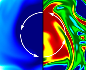
Figure 3 shows contours of the instantaneous axial velocity $u^+_z$ (left half of each panel) and instantaneous axial vorticity $\omega ^+_z$ (right half of each panel) in the cross-stream plane of flows at different rotation numbers. Here, the axial vorticity is defined as $\omega _z = [\partial (r u_\beta )/\partial r-\partial u_r/\partial \beta ]/r$. All contours are depicted at the same axial streamwise location of $z/R = 20{\rm \pi}$ and the same time instant of $t = 20.38$ LETOTs. As is clear from the left half of figure 3(a), in a non-rotating pipe, the flow structures show ‘mushroom patterns’ in the near-wall region where several pairs of small counter-rotating vortices are observed. From figure 3(b), it is observed that because of the axial system rotation imposed (at $Ro_b = 4$), a large counterclockwise-rotating secondary-flow structure appears at the pipe centre, clearly indicated by the contours of positively valued $\omega ^+_z$ (shown in red). As the rotation number continues to increase to $Ro_b = 14$ as shown in figure 3(c), the secondary flow structures indicated by the positively valued $\omega ^+_z$ become the most intense, significantly stretched in the azimuthal direction. The counterclockwise-rotating secondary-flow structures observed at relatively high rotation numbers are the so-called Taylor columns, which become increasingly elongated in the axial direction as the rotation number is increased.

Figure 3.

(a)–(d) Cross-stream view of instantaneous axial velocity $u^+_z$ (left half of each panel) and instantaneous axial vorticity $\omega ^+_z$ (right half of each panel) of the non-rotating ($Ro_b = 0$) and rotating ($Ro_b = 4$, 14 and 20) pipe flows, respectively. White arrows indicate the counterclockwise rotating direction of the secondary flow. All contours are plotted at the same axial location (at $z/R = 20{\rm \pi}$) and the same time instant (at $t = 20.38$ LETOTs). The values of $u_z$ and $\omega _z$ have been non-dimensionalised using $u_\tau$. Results are based on test cases of the longest pipes at corresponding rotation numbers listed in table 1.

3.2. Mean flow fields

Figure 4 compares the cross-stream distributions of the mean axial velocity $\langle u_z \rangle ^+$ and TKE ($k^+=\langle u'_i u'_i\rangle /2$) of four different rotation numbers. Given the axial symmetry of the flow field, only a quarter of the domain is plotted for each rotation number to facilitate a direct comparison. In figure 4(a), the contours of $\langle u_z \rangle ^+$ are superimposed with mean cross-stream velocity vectors for $Ro_b = 0$, 1, 6 and 20. In figure 4(b), the contour plots of $k^+$ are based on rotation numbers $Ro_b = 0$, 1, 14 and 20. By comparing the mean flow patterns at $Ro_b = 0$ and 1 shown in figure 4(a), it can be seen that as soon as the system rotation is imposed, mean secondary-flow motion occurs, behaving as counterclockwise rotations as indicated by the mean cross-stream velocity vectors. From figure 4(a), it is observed that in general, the magnitude of $\langle u_z\rangle ^+$ increases monotonically as the pipe centre is approached for both rotating and non-rotating flow cases. The magnitude of $\langle u_z \rangle ^+$ at the pipe centre reaches its maximum at $Ro_b = 6$. However, as the rotation number further increases from $Ro_b = 6$ to 20, the magnitude of $\langle u_z \rangle ^+$ reduces. This non-monotonic trend in the value of $\langle u_z \rangle ^+$ with an increasing rotation number is interesting, and will be studied further by examining the evolution of the bulk mean velocity $U_b^+$ with $Ro_b$. The variation of the TKE distribution in response to an increasing rotation number also exhibits an interesting trend. As shown in figure 4(b), for a non-rotating pipe flow ($Ro_b = 0$), the peak value of $k^+$ occurs in the buffer layer (at approximately $y^+ = 15$). Clearly, as the value of $Ro_b$ increases, the magnitude of $k^+$ increases in general and, furthermore, the radial distribution of the $k^+$ value varies. More specifically, as the rotation number is increased to $Ro_b = 14$, the peak value of $k^+$ shifts to the pipe centre, a pattern that is in sharp contrast to that of the non-rotating flow ($Ro_b = 0$). As the rotation number continues to increase from $Ro_b = 14$ to 20, the region of large $k^+$ values expands slightly at the pipe centre.

Figure 4.

Cross-stream view of (a) mean axial velocity $\langle u_z\rangle ^+$ and (b) TKE $k^+$ at four different rotation numbers for $Ro_b = 0\unicode{x2013}20$. The direction of the system rotation is clockwise, identical to that shown in figure 3. In panel (a), the contours are superimposed with mean cross-stream velocity vectors indicated by black arrows. The values of $\langle u_z\rangle ^+$ and $k^+$ have been non-dimensionalised based on $u_\tau$. Results are based on test cases of the longest pipes at corresponding rotation numbers listed in table 1.

Figure 5 compares the profiles of the mean axial velocity $\langle u_z\rangle ^+$, mean swirl velocity $r\langle u_\beta \rangle ^+ / R$ and mean axial vorticity $\langle \omega _z\rangle ^+$ with respect to the non-dimensional wall-normal distance ($y$) of the eight test cases of table 1. Given its axial symmetry, only one half the profile of $\langle u_z\rangle ^+$ is plotted in figure 5(a), which varies from the pipe wall to the pipe centre (for $y\in [0, 1]$). From figure 5(a), it is evident that the magnitude of $\langle u_z\rangle ^+$ varies non-monotonically with an increasing $Ro_b$ value. At the pipe centre, the peak value of $\langle u_z\rangle ^+$ increases when the rotation number rises from $Ro_b = 0$ to 6, and reaches its maximum at $Ro_b = 6$ with a magnitude that is $40.19\,\%$ higher than that of the non-rotating pipe flow. As $Ro_b$ continues to increase from 6 to 20, the peak value of $\langle u_z\rangle ^+$ reduces, which however is still larger than that of the non-rotating pipe flow ($Ro_b = 0$). These observations are qualitatively consistent with figure 4(a). From the subpanel of figure 5(b), it is clear that the profile of $\langle u_\beta \rangle ^+$ is zero at both the pipe wall and pipe centre. In addition, it is interesting to observe from figure 5(b,c) that both $r\langle u_\beta \rangle ^+ / R$ and $\langle \omega _z\rangle ^+$ reach their maxima at $Ro_b = 10$, and the peak of $r\langle u_\beta \rangle ^+ / R$ is located at $y \approx 0.4$ where the mean axial vorticity $\langle \omega _z\rangle ^+$ is zero identically.

Figure 5.

Profiles of (a) mean axial velocity $\langle u_z\rangle ^+$, (b) mean swirl velocity $r\langle u_\beta \rangle ^+ / R$ and (c) mean axial vorticity $\langle \omega _z\rangle ^+$ at eight rotation numbers for $Ro_b = 0$–20 based on test cases listed in table 1. In panel (b), the profiles of $\langle u_\beta \rangle ^+$ at different rotation numbers are displayed using a subpanel. In panels (b,c), the pink vertical dash-dotted line demarcates the location of zero value of $\langle \omega _z\rangle ^+$ occurring at $y = 0.4$. All values have been non-dimensionalised by $u_\tau$.

Figure 6 compares the bulk mean velocity $U^+_b$ and volume-averaged TKE $k^+_m$ at varying rotation numbers based on the test cases listed in table 1. In figure 6(a), the profile of $U^+_b$ peaks at $Ro_b = 2$ (or generally in the range of $Ro_b\in [1,6]$), with a magnitude that is $10.33\,\%$ higher than that of the non-rotating pipe flow. As the rotation number is increased beyond 6, the magnitude of $U^+_b$ decreases significantly. At the highest rotation number $Ro_b = 20$, the value of $U_b^+$ is 12.32 % lower than that of the non-rotating flow. The monotonic decreasing trend of $U_b^+$ with respect to an increasing value of $Ro_b$ (at high rotation numbers of $Ro_b\ge 6$) is vividly demonstrated in figure 4(a), and is also consistent with the trend of the mean axial velocity profiles of $\langle u_z\rangle ^+$ shown in figure 5(a) and the result of Orlandi & Ebstein (Reference Orlandi and Ebstein2000). From figure 6(b), the value of $k_m^+$ increases as the rotation number increases in general, and reaches its maximum at $Ro_b = 14$. However, as the rotation number is increased from $Ro_b = 14$ to 20, the value of $k^+_m$ varies little. We explain later that axial rotation enhances the magnitudes of $\langle u'_r u'_r\rangle ^+$ and $\langle u'_\beta u'_\beta \rangle ^+$, which subsequently make a positive contribution to the value of $k^+_m$.

Figure 6.

Profiles of (a) bulk mean velocity $U^+_b$ and (b) volume-averaged TKE $k^+_m$ with respect to the rotation number $Ro_b$. The values of $U^+_b$ and $k^+_m$ have been non-dimensionalised based on $u_\tau$. Results are based on test cases of the longest pipes at corresponding rotation numbers listed in table 1.

3.3. Reynolds stresses

Figure 7 compares the profiles of six Reynolds stresses $\langle u'_z u'_z \rangle ^+$, $\langle u'_r u'_r \rangle ^+$, $\langle u'_\beta u'_\beta \rangle ^+$, $\langle u'_r u'_z \rangle ^+$, $\langle u'_r u'_\beta \rangle ^+$ and $\langle u'_\beta u'_z \rangle ^+$ at eight rotation numbers of $Ro_b = 0\unicode{x2013}20$ based on test cases of table 1. All these Reynolds stress profiles shown are axially symmetrical about the pipe centre (located at $y=1.0$). As shown in figure 7(a), the profile of $\langle u'_z u'_z \rangle ^+$ peaks at $y = 0.083$ (or $y^+ \approx 15$) in the near-wall region of the non-rotating pipe flow. As the rotation number is increased, the magnitude of $\langle u'_z u'_z \rangle ^+$ reduces monotonically in the near-wall region of the pipe. Furthermore, the peak of $\langle u'_z u'_z \rangle ^+$ moves towards the pipe centre as $Ro_b$ increases. The lowest and highest peak values occur at $Ro_b = 4$ and 14, respectively, which are 15.01 % and 4.57 % lower than that of the non-rotating pipe flow ($Ro_b = 0$). In addition, it is interesting to observe that the magnitude of $\langle u'_z u'_z \rangle ^+$ increases monotonically with an increasing rotation number at the pipe centre. At $Ro_b = 20$, the magnitude of $\langle u'_z u'_z \rangle ^+$ increases by more than fivefold in comparison with the non-rotating flow ($Ro_b = 0$). The observations of the apparent migration of the peak of $\langle u'_z u'_z \rangle ^+$ towards the pipe centre at higher rotation numbers (for $Ro_b\ge 6$) and the monotonic increasing trend of the magnitude of $\langle u'_z u'_z \rangle ^+$ with an increasing rotation number at the pipe centre are the result of Taylor columns. The appearance of the Taylor columns at moderate and high rotation numbers also significantly affects the physical features of the mean flow field, e.g. the reduction of the bulk mean velocity $U_b^+$ with an increasing rotation number shown previously in figure 6(a). The characteristics of these two types of coherent flow structures, hairpins and Taylor columns, are studied in detail in both physical and spectral spaces in §§ 3.4 and 3.6.

Figure 7.

Profiles of six Reynolds stresses (a) $\langle u'_z u'_z \rangle ^+$, (b) $\langle u'_r u'_r \rangle ^+$, (c) $\langle u'_\beta u'_\beta \rangle ^+$, (d) $\langle u'_r u'_z \rangle ^+$, (e) $\langle u'_r u'_\beta \rangle ^+$ and (f) $\langle u'_\beta u'_z \rangle ^+$ at eight different rotation numbers for $Ro_b = 0\unicode{x2013}20$ based on test cases of table 1. Pink arrows point to the direction of an increasing rotating effect. All values are non-dimensionalised by $u^2_\tau$.

As is clear in figure 7(b,c), the magnitudes of $\langle u'_r u'_r \rangle ^+$ and $\langle u'_\beta u'_\beta \rangle ^+$ increase monotonically in the pipe centre as the rotation number is increased. Furthermore, as the rotation number rises, the profile of $\langle u_r' u_r' \rangle ^+$ evolves from a dual-peak pattern to a single-peak pattern (over the entire radial direction along a diameter across the pipe), but that of $\langle u'_\beta u'_\beta \rangle ^+$ turns into a triple-peak pattern over the full range of a diameter. In response to the system rotation imposed, secondary flows are induced, which tend to enhance the general levels of $\langle u'_z u'_z \rangle ^+$, $\langle u'_r u'_r \rangle ^+$ and $\langle u'_\beta u'_\beta \rangle ^+$, especially in the central region of the pipe. As a result, the level of the volume-averaged TKE $k^+_m$, shown previously in figure 6(b), enhances as the rotation number increases within the range of this study (for $Ro_b\in [0, 20]$).

From figure 7(d), it is clear that the profile of $\langle u'_r u'_z \rangle ^+$ is approximately linear and symmetrical in the central region of the circular pipe for both non-rotating and rotating flows. For the non-rotating flow case, the profile of $\langle u'_r u'_z\rangle ^+$ peaks at $y = 0.177$ (or $y^+ \approx 32$). However, as the rotation number is increased, the peak position of $\langle u_r' u_z' \rangle ^+$ shifts slightly towards the wall, with its profile being relatively insensitive to the rotation number. For a non-rotating flow, it is well-known that $\langle u'_r u'_\beta \rangle ^+ \equiv 0$ and $\langle u'_\beta u'_z \rangle ^+ \equiv 0$ hold strictly due to the axial symmetry of the flow. However, this is not the case for an axially rotating pipe flow. As is evident in figure 7(e,f), both these Reynolds shear stress components are non-trivial in an axially rotating pipe flow, albeit their magnitudes are one order of magnitude smaller than those of the other four Reynolds normal and shear stress components. Furthermore, as shown in figure 7(e), an approximately linear behaviour can be observed in the profile of $\langle u'_r u'_\beta \rangle ^+$ as soon as the axial system rotation is imposed (for $Ro_b \ge 1$), which is a consequence of clockwise system rotation of the pipe. This observation is consistent with the finding by Orlandi & Fatica (Reference Orlandi and Fatica1997). Figure 7(f) shows the radial profile of $\langle u'_\beta u'_z \rangle ^+$. Clearly, the value of $\langle u'_\beta u'_z\rangle ^+$ is zero identically at the pipe wall ($y = 0$) and at the pipe centre ($y = 1.0$), due to the no-slip and axial-symmetry flow conditions, respectively. As the rotation number is increased, the amplitude of $\langle u'_\beta u'_z\rangle ^+$ increases monotonically. At high rotation numbers of $Ro_b \ge 14$, it is interesting to observe that the value of $\langle u'_\beta u'_z\rangle ^+$ changes sign three times within half a radial domain (for $y \in [0,1]$), such that there are five zero-crossing points along the entire radial direction of a diameter.

The behaviours of the three components of Reynolds shear stresses associated with figure 7(d–f) can be further analysed through their corresponding shear stress balance equations. Assuming that the flow is fully developed in the axial direction, and statistically homogeneous in the axial and azimuthal directions, the following equations can be obtained from the $z$-, $\beta$- and $r$-components of the momentum equation (2.2) after applying turbulence decomposition (i.e. $u_i = \langle u_i\rangle + u_i'$) to the velocity (Speziale et al. Reference Speziale, Younis and Berger2000)

(3.1)\begin{gather} \frac{\nu}{r}\frac{{\rm d}}{{\rm d} r}\left( r\frac{{\rm d}\langle u_z \rangle}{{\rm d} r} \right) - \frac{1}{r}\frac{{\rm d} \left( r \langle u'_r u'_z \rangle \right)}{{\rm d} r} = \varPi, \end{gather}

(3.2)\begin{gather} \nu\frac{{\rm d}}{{\rm d} r}\left[\frac{1}{r}\frac{{\rm d}\left( r \langle u_\beta \rangle\right)}{{\rm d} r}\right] - \frac{1}{r}\frac{{\rm d} \left( r \langle u'_r u'_\beta \rangle \right)}{{\rm d} r} - \frac{\langle u_r' u_\beta' \rangle}{r} = 0 , \end{gather}

(3.3)\begin{gather} \langle u'_\beta u'_\beta \rangle - \langle u'_r u'_r \rangle ={-}\langle u_\beta \rangle \langle u_\beta \rangle + r\left(\frac{1}{\rho}\frac{{\rm d} \langle p \rangle}{{\rm d} r} + \frac{{\rm d}\langle u'_r u'_r \rangle}{{\rm d} r} - 2\varOmega_z\langle u_\beta \rangle \right). \end{gather}

Note that in the derivation of (3.2) from the $\beta$-component of the momentum equation, the mean azimuthal Coriolis force $\langle F_\beta \rangle$ is zero identically because $\langle u_r \rangle \equiv 0$. Both viscous shear and Reynolds shear stresses vanish from (3.3), the simplified $r$-component of the momentum equation. From (3.3), it is clear that at pipe centre (where $r = 0$ or $y = 1.0$), $\langle u'_\beta u'_\beta \rangle - \langle u'_r u'_r \rangle = 0$. This explains the observation in figure 7(b,c) that the trends and magnitudes of $\langle u'_\beta u'_\beta \rangle$ and $\langle u'_r u'_r \rangle$ become increasingly similar as the pipe centre is approached. In a fully developed pipe flow, $\tau _{\beta z}^{vis} = \tau _{z\beta }^{vis}\equiv 0$. In (3.1) and (3.2), the remaining two non-trivial mean viscous shear stresses are defined as (Reich & Beer Reference Reich and Beer1989)

(3.4a,b)\begin{equation} \tau_{rz}^{vis} = \nu \frac{\partial \langle u_z\rangle}{\partial r} \quad \text{and} \quad \tau_{r\beta}^{vis} = \nu r \frac{\partial}{\partial r} \left(\frac{\langle u_\beta\rangle}{r}\right), \end{equation}

respectively. The total shear stresses balance as

(3.5)\begin{equation} \tau_{ri}^{tot} = \tau_{ri}^{vis} - \langle u'_r u'_i \rangle , \end{equation}

where $i$ denotes $z$ or $\beta$. The budget balance of total shear stresses in non-dimensional forms (i.e. $\tau _{rz}^{tot +}$ and $\tau _{r\beta }^{tot +})$ is displayed in figure 8. The linear behaviour of $\tau _{rz}^{tot +}$ is evident from (3.1), whose non-dimensional form may be expressed as

(3.6)\begin{equation} \tau_{rz}^{tot+}= \tau_{rz}^{vis+} - \langle u'_r u'_z \rangle^+ = y-1 , \end{equation}

in the context of an axially rotating pipe flow. From figure 8(a), the profile of $-\langle u'_r u'_z \rangle ^+$ changes slightly in its shape as the rotation number is increased from $Ro_b = 2$ to 20. The reason the profile of $-\langle u'_r u'_z \rangle ^+$ is insensitive to $Ro_b$ is that its value is linearly related to the viscous shear stress such that the total shear stress varies as $\tau _{rz}^{tot+}=y-1$ for both rotating and non-rotating pipe flows. From (3.6), it is understood that at the wall ($y=0$) $\langle u'_r u'_z \rangle ^+|_w\equiv 0$, and so the non-dimensional wall-shear stress becomes $\tau _w^+=\tau _{rz}^{vis+}|_w \equiv -1$. Therefore, for axially rotating pipe flows of different rotation numbers, the wall shear stress $\tau _w$ is expected to be constant, which is evidenced by the stable values of the calculated wall friction number $Re_\tau ^A$ listed in table 1. Furthermore, because the wall shear stress $\tau _w$ is constant, it is inferred that the skin friction coefficient, defined as $C_f=\tau _w/(\rho U_b^2/2)$, is proportional to $U_b^{-2}$ with the value of $U_b$ given in figure 6(a).

Figure 8.

Budget profiles of mean shear stress $\tau _{rz}^+$ and $\tau _{r\beta }^+$ at two rotation numbers $Ro_b = 2$ and 20 based on test cases of the longest pipes of table 1. All shear stress budget terms are non-dimensionalised by $u^2_\tau$. Panel (a) shows radial–axial shear stress components ($\tau _{rz}^{vis +}$ and $-\langle u'_r u'_z \rangle ^+$). Panel (b) shows radial–azimuthal shear stress components ($\tau _{r\beta }^{vis +}$ and $-\langle u'_r u'_\beta \rangle ^+$).

From figure 8(b), it is interesting to observe that the profile of $\tau _{r\beta }^{vis+}$ is almost a mirror reflection of that of Reynolds stress $- \langle u'_r u'_\beta \rangle ^+$ such that the total shear stress is zero, i.e. $\tau _{r\beta }^{tot +} = 0$. This is an expected feature, which can be strictly proven as follows. Equation (3.2) is derived from the $\beta$-component of the momentum equation, which can also be written as $\boldsymbol {\nabla }\boldsymbol {\cdot } \tau _{r\beta }^{tot} = 0$, or

(3.7)\begin{equation} \frac{\partial \tau_{r\beta}^{tot}}{\partial r}+\frac{2\tau_{r\beta}^{tot}}{r} = 0 . \end{equation}

The solution to the above equation is

(3.8)\begin{equation} \tau_{r\beta}^{tot} = \frac{C}{r^2}, \end{equation}

where $C$ is a constant. The regularity condition at the pipe centre requires that $C \equiv 0$. As such,

(3.9a,b)\begin{equation} \tau_{r\beta}^{tot}\equiv 0 \quad \mathrm{and}\quad \tau_{r\beta}^{vis} \equiv \langle u'_r u'_\beta\rangle , \end{equation}

hold rigorously in an axially rotating pipe flow. This is an interesting result, which indicates that the total $r$–$\beta$ shear stress is zero identically, such that the viscous shear stress is always balanced by the turbulent shear stress (in an $r$–$\beta$ plane) at all rotation numbers. This mechanism gives an analytical explanation to the mirror effect between the profiles of $\tau _{r\beta }^{vis +}$ and $-\langle u'_r u'_\beta \rangle ^+$ as observed in figure 8(b).

3.4. Two-point correlations and spectral analysis

Figure 9 compares the two-point autocorrelation coefficients of three velocity components $R_{zz}$, $R_{rr}$ and $R_{\beta \beta }$ at different rotation numbers based on the eight test cases of table 1. All coefficients are determined along the axial direction at wall-normal position $y^+ \approx 15$, where Reynolds stress component $\langle u'_z u'_z\rangle ^+$ peaks in the context of a non-rotating pipe flow. The two-point autocorrelation coefficient is defined as

(3.10)\begin{equation} R_{ii}(\Delta z) = \frac{\langle u'_i(r, \beta, z, t)u'_i(r, \beta, z+\Delta z, t)\rangle}{\langle u'_i(r, \beta, z, t)u'_i(r, \beta, z, t) \rangle}, \end{equation}

where $i$ indicates the three directions (i.e. $r$, $\beta$ and $z$) of the cylindrical coordinate system, and no summation convention is implied in this equation. In figure 9(a,c), a partially enlarged panel is also displayed in a semi-logarithmic coordinate in order to clearly display the variations of $R_{zz}$ and $R_{\beta \beta }$ for smaller two-point separations ($\Delta z/R$). From figure 9(b), it is apparent that the profiles of the radial two-point autocorrelation coefficient $R_{rr}$ at all rotation numbers approach zero rather rapidly as the two-point separation $\Delta z/R$ increases. By contrast, the axial and azimuthal two-point correlation coefficients $R_{zz}$ and $R_{\beta \beta }$ shown in figure 9(a,c) are more sensitive to the rotation number, as their values increase monotonically with an increasing value of $Ro_b$ for small two-point separations. Furthermore, it is very interesting to observe a quasi-periodical pattern in the profiles of $R_{zz}$ and $R_{\beta \beta }$ in figures 9(a) and 9(c), respectively. The spatial periods become larger as the rotation number $Ro_b$ increases. It is evident that the axial scales of the most energetic secondary flow structures (i.e. Taylor columns) induced by the Coriolis force increase monotonically as the rotation number is increased. The quasi-periodical patterns in the profiles of $R_{zz}$ and $R_{\beta \beta }$ are most apparent at high rotation numbers.

Figure 9.

Profiles of two-point autocorrelation coefficients (a) axial component $R_{zz}$, (b) radial component $R_{rr}$ and (c) azimuthal component $R_{\beta \beta }$ for the eight test cases of different rotation numbers $Ro_b$, calculated along the streamwise direction at wall-normal position $y = 0.083$ (or $y^+ \approx 15$). Pink arrows in the partially enlarged panels (a,c) indicate the direction of an increasing rotation number. Results are based on test cases of the longest pipes at corresponding rotation numbers listed in table 1.

As mentioned earlier, there are two main types of flow structure in an axially rotating pipe flow. The first type is streaky structures near the wall (or hairpins) that are typical of the turbulent boundary layer of a pipe flow (rotating or not). The second type is Taylor columns similar to those observed in rotating isotropic turbulence (see, e.g., Bartello et al. Reference Bartello, Métais and Lesieur1994; Gallet Reference Gallet2015; van Kan & Alexakis Reference van Kan and Alexakis2020; Pestana & Hickel Reference Pestana and Hickel2020). However, compared with rotating isotropic turbulence, a turbulent pipe flow is bounded peripherally by the pipe wall of curvature $1/R$. From the profiles of $R_{zz}$ and $R_{\beta \beta }$, it is inferred that the Taylor columns in an axially rotating pipe flow exhibit a spiral pattern, which elongate in the axial direction and spin in the azimuthal direction. In fact, the axial quasi-periodicity of the two-point autocorrelation ($R_{\beta \beta }$) observed in figure 9(c) is a consequence of the counterclockwise spinning motion of Taylor columns demonstrated previously in figures 3, 4(a) and 5(b). Furthermore, both axial and azimuthal motions of Taylor columns are quasi-periodic in the axial direction, which are evident in figure 9(a,c). A vivid analogy for describing the instantaneous shape of Taylor columns in an axially rotating pipe flow is ‘a bundle of hemp ropes’, twisted together with many smaller individual ropes of different brand names (as such, each can have its own axial and azimuthal periods). As turbulence structures, small Taylor columns can be destroyed by dissipation and transported by diffusion and convection in a viscous flow.

The analysis of Taylor columns can be refined through a spectral analysis, which will show that Taylor columns have two characteristic axial length scales. To demonstrate, figure 10 compares the profiles of the premultiplied axial spectra of axial, radial and azimuthal velocity fluctuations (i.e. $k^+_z\tilde {E}^+_{zz}$, $k^+_z\tilde {E}^+_{rr}$ and $k^+_z\tilde {E}^+_{\beta \beta }$, respectively) of the eight test cases of the longest pipes of table 1. All profiles are calculated at wall-normal position $y^+ \approx 15$, where the axial Reynolds normal stress peaks in the context of a non-rotating pipe flow. The 1-D axial energy spectrum of velocity fluctuations is defined as

(3.11)\begin{equation} \tilde{E}_{ii}(k_z) = \text{Re}\left\{ \overline{\widehat{u'_i}^*\widehat{u'_i}} \right\} , \end{equation}

where the index $i$ denotes $r$, $\beta$ or $z$ of the cylindrical coordinate system, and no summation convention is implied. An overbar represents temporal averaging. The operator Re$\{{\cdot }\}$ and superscript * denote the real part and conjugate of a complex number, respectively. A hat denotes Fourier transform in the axial direction of an arbitrary variable $\phi (r, \beta, k_z, t)$, i.e.

(3.12)\begin{equation} \hat\phi(r, \beta, k_z, t) = \frac{1}{L_z}\int_0^{L_z}\phi(r, \beta, z, t){\rm e}^{- {\underline{{\rm i}}}\, k_z z}\,{\rm d}z, \end{equation}

where $\underline {{\rm i}} = \sqrt {-1}$ is the imaginary unit and $k_z = n_zk_{0z}$ is the axial wavenumber, with $n_z \in [-N_z/2, N_z/2-1]$ being an integer and $k_{z0} = 2{\rm \pi} / L_z$ being the smallest positive wavenumber. The axial wavelength is defined as $\lambda _z = 2{\rm \pi} /k_z$, non-dimensionalised as $\lambda ^+_z = \lambda _z u_\tau / \nu$.

Figure 10.

Profiles of premultiplied (a) axial $k^+_z\tilde {E}^+_{zz}$, (b) radial $k^+_z\tilde {E}^+_{rr}$ and (c) azimuthal $k^+_z\tilde {E}^+_{\beta \beta }$ velocity spectra at eight different rotation numbers for $Ro_b = 0\unicode{x2013}20$, calculated along the streamwise direction at wall-normal position $y = 0.083$ (or $y^+ \approx 15$). Pink arrow points to the direction of an increasing rotation number. For clarity, the peaks of premultiplied spectra ($I$, $II$ and $III$) are labelled only for the two highest rotation numbers $Ro_b=14$ and 20. Results are based on test cases of the longest pipes at corresponding rotation numbers listed in table 1.

For the premultiplied axial velocity spectrum $k^+_z\tilde {E}^+_{zz}$, it is evident in figure 10(a) that the mode of its dome peak (corresponding to the characteristic length scale of the most energetic eddies) of the non-rotating pipe flow ($Ro_b = 0$) is located within $\lambda ^+_z \in [530, 2450]$ at $y^+ \approx 15$ in the near-wall region, where axial Reynolds normal stress peaks. This peak of $k^+_z\tilde {E}^+_{zz}$ is a consequence of near-wall streaks of the boundary layer developing over the pipe wall. The formation of this peak does not rely on axial system rotation, but rather, it is a characteristic of a turbulent boundary layer commonly found in wall-bounded flows over flat plates (see, e.g., Zhou et al. Reference Zhou, Adrian, Balachandar and Kendall1999; Adrian Reference Adrian2007; Wu & Moin Reference Wu and Moin2009) or in non-rotating pipe flows (see, e.g., Wu & Moin Reference Wu and Moin2008; Wu et al. Reference Wu, Baltzer and Adrian2012; Baltzer, Adrian & Wu Reference Baltzer, Adrian and Wu2013). This peak of the premultiplied axial velocity spectrum $k^+_z\tilde {E}^+_{zz}$ is denoted as peak ‘$I$’ hereafter, and for a specific rotation number (e.g. $Ro_b =14$ or 20), it is indicated using the rotation number as the subscript (as $I_{14}$ or $I_{20}$, respectively). As the rotation number is increased from $Ro_b = 0$ to 20, the magnitude of the first peak ($I$) of $k^+_z\tilde {E}^+_{zz}$ decreases monotonically. Meanwhile, the mode of the first peak moves towards larger wavelengths, leading to an increasingly broadband vortical scales in the axial direction as the rotation number is increased. At the highest rotation number $Ro_b = 20$, the wavelengths of the first peak range within $\lambda ^+_z \in [4840, 5660]$.

From figure 10(a), it is interesting to see that at high rotation numbers (for $Ro_b \ge 10$), there are two additional peaks (denoted as peaks ‘$II$’ and ‘$III$’) in addition to peak $I$ in the profiles of the premultiplied axial velocity spectrum $k^+_z\tilde {E}^+_{zz}$. Similarly, peaks of different rotation numbers are differentiated symbolically by using rotation numbers as the subscripts (e.g. $II_{20}$ or $III_{20}$ for the case of $Ro_b = 20$). The appearance of peaks $II$ and $III$ in the profiles of $k^+_z\tilde {E}^+_{zz}$ is due to the presence of Taylor columns, which are elongated in the axial direction and spin in the azimuthal direction, as discussed previously through the analysis of two-point autocorrelation coefficients $R_{zz}$ and $R_{\beta \beta }$ associated with figures 9(a) and 9(c), respectively. Using the examples of $Ro_b = 14$ and 20, the peak magnitudes follow an ascending order, i.e. ‘$I_{14} < II_{14}< III_{14}$’ and ‘$I_{20} < II_{20}< III_{20}$.’ This indicates that at high rotation numbers, the share of TKE held by Taylor columns associated with peaks $II$ and $III$ (and especially with peak $III$) is much larger than that held by streaks at this radial position. Within the range of the rotation numbers tested here, all three peaks of $k^+_z\tilde {E}^+_{zz}$ have been well captured. The premultiplied energy spectrum loss (in terms of the percentage of its peak value) is less than 20 % at their cutoff wavelengths. It is also interesting to observe that there is no apparent distinction between the second and third peaks at moderate rotation numbers of $Ro_b = 4$ and 6, as the two types (axial and azimuthal) of structures of Taylor columns are still evolving temporally and spatially. This indicates that Taylor columns start to occur at moderate rotation numbers with similar characteristic axial wavelengths. However, as the rotation number continues to increase, Taylor columns evolve spatially to feature two distinct axial characteristic wavelengths, corresponding to modal values of peaks $II$ and $III$ of $k^+_z\tilde {E}^+_{zz}$. Furthermore, both characteristic axial wavelengths of Taylor columns increase as the rotation number is increased.

Given that the characteristic axial length scale of energetic eddy motions grows with an increasing rotation number, the pipe length is extended from $L_z = 30{\rm \pi} R$ to $180{\rm \pi} R$ as rotation number increases from $Ro_b = 0$ to 20 (see table 1). As shown in figure 10(a), the cutoff wavelength varies from $(\lambda ^+_z)_{{CF}} = 16964.6$ at $Ro_b = 0$ to $(\lambda ^+_z)_{{CF}} = 101787.6$ at $Ro_b = 20$. At the cutoff wavelength, the premultiplied energy spectrum loss varies from 10.33 % at $Ro_b = 4$ to 19.81 % at $Ro_b = 1$. Clearly, if the short pipe of $L_z = 25R$ (or $7.958{\rm \pi} R$) is used (as in Orlandi & Ebstein Reference Orlandi and Ebstein2000), the prediction of the largest peak $III_{20}$ of $k^+_z\tilde {E}^+_{zz}$ that is characteristic of Taylor columns would be missed entirely. It should be indicated that it is neither necessary nor realistic to fully prevent premultiplied energy spectrum loss at the cutoff wavelength in either a DNS or an experiment, as it implies usage of a pipe of infinite length. Furthermore, flow structures of large wavelengths far beyond the mode of the premultiplied spectrum typically possess very low TKE. However, it is important to ensure that all dominant modes of premultiplied spectra are captured in a DNS, LES or physical experiment, which correspond to the characteristic length scales of the most energetic eddy motions. In practice, for example, the premultiplied energy spectrum loss at the cutoff wavelength is often kept lower than 5/8 or 3/8 of its modal value (i.e. $0.625\max (k_z^+\tilde {E}^+_{ii})$ or $0.375\max (k_z^+\tilde {E}^+_{ii})$ for moderate and relatively high-precision requirements, respectively) in DNS studies of turbulent plane-channel flows (Hoyas & Jiménez Reference Hoyas and Jiménez2006; Avsarkisov et al. Reference Avsarkisov, Hoyas, Oberlack and García-Galache2014; Yang & Wang Reference Yang and Wang2018; Bagheri, Wang & Yang Reference Bagheri, Wang and Yang2020).

In contrast to the general trend of the premultiplied axial velocity spectrum $k^+_z\tilde {E}^+_{zz}$ shown in figure 10(a), the magnitude of the premultiplied radial velocity spectrum $k^+_z\tilde {E}^+_{rr}$ increases monotonically as the rotation number is increased, a pattern that is apparent in figure 10(b). The presence of the dominant peak of $k^+_z\tilde {E}^+_{rr}$ at this near-wall position of approximately $y^+ = 15$ results from the streaky structures. As shown in figure 10(b), the modal position of $k^+_z\tilde {E}^+_{rr}$ is relatively stable at all eight rotation numbers tested. A careful perusal of the figure indicates that the characteristic axial length scale of the most energetic radial eddy motions as indicated by the mode of $k^+_z\tilde {E}^+_{rr}$ increases from $\lambda _z^+ = 282.74$ to 568.65 as the rotation number is increased from $Ro_b = 0$ to 20.

Figure 10(c) compares the premultiplied azimuthal velocity spectrum $k_z^+\tilde {E}^+_{\beta \beta }$ at eight rotation numbers. Similar to figure 10(a), the number of peaks in the profile of $k_z^+\tilde {E}^+_{\beta \beta }$ varies with the rotation number. At low rotation numbers $Ro_b =0$ and 1, the profile of $k_z^+\tilde {E}^+_{\beta \beta }$ shows only one dominant peak (denoted as $I_0$ and $I_1$, respectively, not labelled in the figure) within the range of $\lambda _z^+ \in [220,600]$, which is a signature of near-wall streaks, shown also at higher rotation numbers at slightly larger wavelengths. However, at moderately high rotation numbers of $Ro_b = 4$ and 6 as shown in figure 10(c), a second sharp peak (denoted as $II_4$ and $II_6$, respectively, not labelled in the figure) appears around $\lambda _z^+ = 4241$ and 4847, which is an indication of the occurrence of Taylor columns. As the rotation number continues to increase, Taylor columns further develop in both axial and azimuthal directions leading to two characteristic axial wavelengths. At higher rotation numbers for $Ro_b\ge 10$, two dominant peaks ($II$ and $III$) of Taylor columns (besides the existing reduced peak $I$ of the streaks) are identified. At the two highest rotation numbers tested, these two characteristic peaks of Taylor columns are labelled as $II_{14}$ and $III_{14}$ (at $Ro_b = 14$) and $II_{20}$ and $III_{20}$ (at $Ro_b = 20$) in figure 10(c). By comparing figures 10(a) and 10(c), it is clear that the pipe flow motion is dominated by streaks (or hairpins, signified by peak $I$) at low rotation numbers for $Ro_b\in [0, 2]$, Taylor columns of one single characteristic wavelength (signified by peak $II$) at moderate rotation numbers for $Ro_b\in [4, 6]$ and Taylor columns of two characteristic wavelengths (signified by peaks $II$ and $III$) at high rotation numbers for $Ro_b\in [10, 20]$. The two peaks ($II$ and $III$) of $k_z^+\tilde {E}^+_{zz}$ and $k_z^+\tilde {E}^+_{\beta \beta }$ observed at the high rotation numbers for $Ro_b \ge 10$ are consistent with the quasi-periodic behaviours of $R_{zz}$ and $R_{\beta \beta }$ observed previously in figure 9(a,c).

Thus far, the analysis of the axial premultiplied velocity spectra has been conducted at $y = 0.083$ (or $y^+ \approx 15$) in the near-wall region of the pipe in figure 10. From the previous analysis of figure 7(a), it was observed that the value of $\langle u'_z u'_z \rangle ^+$ peaks at this wall-normal position at $Ro_b=0$, but at $y = 0.566$ (or $y^+ \approx 102$) at $Ro_b = 20$. It would be interesting to further examine the behaviours of the three components of the axial premultiplied velocity spectra at this special wall-normal position of $y = 0.566$, which is demonstrated in figure 11. From this figure, it is seen that all dominant peaks of the axial premultiplied velocity spectra (e.g. peaks $I_{14}$, $II_{14}$ and $III_{14}$ for $Ro_b = 14$, peaks $I_{20}$, $II_{20}$ and $III_{20}$ for $Ro_b = 20$) have been well captured based on the eight test cases of the longest pipes listed in table 1. As shown in figure 11(a), the largest premultiplied energy spectrum loss is about 21.37 % (in terms of the percentage of its peak value) at $Ro_b = 1$ at the cutoff wavelength.

Figure 11.

Profiles of premultiplied (a) axial $k^+_z\tilde {E}^+_{zz}$, (b) radial $k^+_z\tilde {E}^+_{rr}$ and (c) azimuthal $k^+_z\tilde {E}^+_{\beta \beta }$ velocity spectra at eight different rotation numbers for $Ro_b = 0\unicode{x2013}20$, calculated along the streamwise direction at wall-normal position $y = 0.566$ (or $y^+ \approx 102$). For clarity, the peaks of premultiplied spectra ($I$, $II$ and $III$) are labelled only for the two highest rotation numbers $Ro_b=14$ and 20. Results are based on test cases of the longest pipes at corresponding rotation numbers listed in table 1.

By comparing figure 11 with figure 10, it is clear that the profile patterns of all three components of the axial premultiplied velocity spectra change considerably as the elevation increases from $y = 0.083$ to 0.566. As shown in figure 11(a), the magnitudes of peaks $II$ and $III$ of $k^+_z\tilde {E}^+_{zz}$ are significantly larger than that of peak $I$ at higher rotation numbers of $Ro_b\ge 10$. This indicates that Taylor columns become increasingly energetic as the distance from the pipe wall increases. Such trend of Taylor columns is more clearly reflected in the profiles of all three axial premultiplied spectra. As shown in figure 10(b), the profile of $k^+_z\tilde {E}^+_{rr}$ has only one dominant peak in the near-wall region (at $y = 0.083$), which is peak $I$ resulted from near-wall streaks of the boundary layer developing over the pipe wall. By contrast, as is evident in figure 11(b), the profile of $k^+_z\tilde {E}^+_{rr}$ is dominated by peaks $II$ and $III$ of Taylor columns at moderate and high rotation numbers of $Ro_b\ge 4$ at a higher elevation of $y = 0.566$. In comparison with the profiles of $k^+_z\tilde {E}^+_{\beta \beta }$ in the near-wall region shown in figure 10(c), those shown in figure 11(c) indicate that the magnitudes of peaks $II$ and $III$ reduce relative to that of peak $I$ as the elevation increases from $y = 0.083$ to 0.566.

Figure 12 shows the profiles of the three components of the axial premultiplied velocity spectra at the pipe centre ($y = 1.0$) where the mean axial velocity value reaches the maximum and the magnitudes of Reynolds normal stresses $\langle u'_r u'_r\rangle$ and $\langle u'_\beta u'_\beta \rangle$ are the maximum. At the pipe centre, $k^+_z\tilde {E}^+_{rr}\equiv k^+_z\tilde {E}^+_{\beta \beta }$. Clearly, all dominant peaks of $k^+_z\tilde {E}^+_{zz}$, $k^+_z\tilde {E}^+_{rr}$ and $k^+_z\tilde {E}^+_{\beta \beta }$ have been well captured at eight rotation numbers based on test cases of the longest pipes listed in table 1. In comparison with figures 10 and 11, it is clear that the peak magnitude of $k^+_z\tilde {E}^+_{zz}$ shown in figure 12 drops as the elevation increases from $y = 0.083$ to 1.0. Furthermore, it is clear that the profile of $k^+_z\tilde {E}^+_{\beta \beta }$ features peak $I$ of hairpins in non-rotating or slowly rotating pipe flows (of low rotation numbers $Ro_b=0\unicode{x2013}2$). However, as the rotation number increases, the profile of $k^+_z\tilde {E}^+_{\beta \beta }$ begins to signify Taylor columns, featuring one single dominant peak $II$ at moderate rotation numbers (of $Ro_b=4\unicode{x2013}6$) but two dominant peaks $II$ and $III$ at high rotation numbers (of $Ro_b \ge 10$).

Figure 12.

Profiles of premultiplied (a) axial $k^+_z\tilde {E}^+_{zz}$, (b) radial $k^+_z\tilde {E}^+_{rr}$ and (c) azimuthal $k^+_z\tilde {E}^+_{\beta \beta }$ velocity spectra at eight different rotation numbers for $Ro_b = 0\unicode{x2013}20$, calculated along the streamwise direction at the pipe centre $y = 1.0$. For clarity, the peaks of premultiplied spectra ($I$, $II$ and $III$) are labelled only for the two highest rotation numbers $Ro_b=14$ and 20. Results are based on test cases of the longest pipes at corresponding rotation numbers listed in table 1.

Figure 13 compares the contour patterns of the non-dimensionalised premultiplied 1-D spectrum of axial velocity fluctuations $k^+_z\tilde {E}^+_{zz}$ as a function of $\lambda _z^+$ and $y^+$ at two rotation numbers $Ro_b =0$ and 20 based on the longest-pipe cases of table 1. The effects of axial system rotation on the generation of Taylor columns are evident by directly contrasting figures 13(a) against 13(b). For the non-rotating pipe flow, there is only one mode located at $(\lambda _z^+,y^+) = (997.4,12.9)$, which corresponds to peak $I_0$. This peak is a consequence of near-wall streaks. However, at the highest rotation number $Ro_b = 20$ as shown in figure 13(b), the presence of all three peaks ($I_{20}$, $II_{20}$ and $III_{20}$) are evident, located at $(\lambda _z^+,y^+) = (7268.5, 63.8)$, $(12719.9, 114.3)$ and $(33919.8, 97.6)$, respectively. In figure 13(a), three regions of high-, intermediate- and low-intensity cores are distinguished by different colours enclosed within three isopleths, corresponding to $0.875\max (k^+_z\tilde {E}^+_{zz})$, $0.625\max (k^+_z\tilde {E}^+_{zz})$ and $0.375\max (k^+_z\tilde {E}^+_{zz})$ (or $7/8$, $5/8$ and $3/8$ of the peak value of $k^+_z\tilde {E}^+_{zz}$, respectively). The high-intensity core within the innermost isopleth of $0.875\max (k^+_z\tilde {E}^+_{zz})$ are associated with the most energetic eddies of the turbulent flow field. Although the low-intensity core enclosed by the outermost isopleth of $0.375\max (k^+_z\tilde {E}^+_{zz})$ corresponds to less-dominant energetic eddies consisting of a wide range wavelengths, it still makes a considerable contribution to the total TKE. Because the TKE is mostly held by Taylor columns at the high rotation number $Ro_b =20$, the magnitude of peak $I_{20}$ is much less than those of peaks $II_{20}$ and $III_{20}$. Therefore, the value of the outermost isopleth is reduced to $0.18\max (k^+_z\tilde {E}^+_{zz})$ in order to have a clear view of the location of peak $I_{20}$. By comparing figures 13(a) and 13(b), it is also seen that the modal position of all three peaks ($I_{20}$, $II_{20}$ and $III_{20}$) are near the pipe centre. At the rotation number is increased from $Ro_b =0$ to 20, the modal position of peak $I$ increases from $y^+ = 12.9$ to 63.8.

Figure 13.

Isopleths of premultiplied axial velocity spectra $k^+_z\tilde {E}^+_{zz}$ with respect to wall-normal coordinate $y^+$ and wavelength $\lambda _z^+$ for the (a) non-rotating ($Ro_b = 0$) and (b) axially rotating ($Ro_b = 20$) pipe flows. The cross symbols ‘$\times$’ demarcate the locations of the three peaks $I$, $II$ and $III$. The three energy levels are distinguished by the innermost, intermediate and outermost isopleths of 87.5 %, 62.5 % and 37.5 % of the peak value $\max (k^+_z\tilde {E}^+_{zz})$ in panel (a), and 87.5 %, 37.5 % and 18.0 % of the peak value $\max (k^+_z\tilde {E}^+_{zz})$ in panel (b), respectively.

Figure 14 compares the profiles of $k^+_z\tilde {E}^+_{zz}$ of $Ro_b =20$ at five wall-normal distances ranging from $y = 0.083$ (near the wall) to $y = 1.0$ (at the pipe centre). The results are based on the case of the longest pipe $L_z=180{\rm \pi} R$. At this high rotation number, it is clear that turbulent flow structures of an axially rotating pipe flow feature predominantly Taylor columns (as indicated by peaks $II_{20}$ and $III_{20}$). From the previous analysis of figures 10–12, it is understood that the modal wavelengths corresponding to peaks $I$, $II$ and $III$ of profiles of $k^+_z\tilde {E}^+_{zz}$, $k^+_z\tilde {E}^+_{rr}$ and $k^+_z\tilde {E}^+_{\beta \beta }$ may vary with wall-normal distance $y$. As is evident in figure 14(a–c), the characteristic wavelength corresponding to peak $II_{20}$ is rather stable (with $\lambda _z^+\approx 12723$) as the elevation ($y$ value) varies. However, the characteristic wavelengths of peaks $I_{20}$ and $III_{20}$ range slightly, which are indicated by a pair of dashed lines and arrows in figure 14(a–c). A careful perusal of figure 14(a,c) indicates that the magnitudes of $k^+_z\tilde {E}^+_{zz}$ and $k^+_z\tilde {E}^+_{\beta \beta }$ are the largest and the smallest, respectively, at $y = 0.566$, which are consistent with the previous observations of a local maximum value of $\langle u'_z u'_z\rangle ^+$ and a local minimum value of $\langle u'_\beta u'_\beta \rangle ^+$ in figure 7(a,c) at a similar wall-normal position, respectively. In figure 14(b), it is shown that the magnitude of $k^+_z\tilde {E}^+_{rr}$ increases as $y$ increases. Such general monotonic trend is consistent with that of $\langle u'_r u'_r\rangle ^+$ observed in figure 7(b). This is an expected feature, simply because the Reynolds stresses relate directly to their premultiplied spectra $k_z \tilde {E}_{ij}$ through integration $\langle u'_i u'_j\rangle = 2\int _0^\infty k_z \tilde {E}_{ij} \,{\rm d}(\ln k_z)$.

Figure 14.

Profiles of premultiplied (a) axial $k^+_z\tilde {E}^+_{zz}$, (b) radial $k^+_z\tilde {E}^+_{rr}$ and (c) azimuthal $k^+_z\tilde {E}^+_{\beta \beta }$ velocity spectra at the highest rotation number $Ro_b = 20$, calculated along the streamwise direction at different wall-normal ($y$) positions, based on the test case of the longest pipe $L_z = 180{\rm \pi} R$.

3.5. Higher-order turbulence statistics

So far, the influence of the Coriolis force on an axially rotating pipe flow has been studied thoroughly through investigations into the mean flow and second-order turbulence statistics. In order to develop a deeper insight into the flow, the third- and fourth-order statistical moments can be further examined. Figure 15 shows the radial profiles of the skewness and flatness factors of three velocity fluctuations, defined as

(3.13a,b)\begin{equation} S(u'_i) = \frac{\langle {u'_i}^3 \rangle}{{\langle {u'_i}^2 \rangle}^{3/2}} \quad \text{and} \quad F(u'_i) = \frac{\langle {u'_i}^4 \rangle}{{\langle {u'_i}^2 \rangle}^2}, \end{equation}

respectively. Here, indices $i=1$, 2 and 3, correspond to cylindrical coordinates $r$, $\beta$ and $z$, respectively, and no summation convention is implied. To study the ejection and sweep events in a circular pipe flow, it is convenient to consider the analogy of a boundary-layer flow developing over a flat plate. Thus, the negative of instantaneous radial velocity fluctuation ($-u'_r$) is used in the calculation of the radial skewness factor $S(-u'_r)$. This greatly facilitates an intuitive near-wall analysis of physical phenomena associated with the skewness factor based on the non-dimensional wall coordinate $y$.

Figure 15.

Profiles of skewness (a,c,e) and flatness factors (b,d,f) of three velocity fluctuations at various rotation numbers of $Ro_b = 0\unicode{x2013}20$: (a) $S(u'_z)$; (b) $F(u'_z)$; (c) $S(-u'_r)$; (d) $F(u'_r)$; (e) $S(u'_\beta )$; (f) $F(u'_\beta )$. The pink dash-dotted line indicates the theoretical values of an ideal Gaussian distribution, which are 0 and 3 for skewness and flatness, respectively. The pink arrow shows a local trend of an increasing rotation number $Ro_b$. Results are based on test cases of the longest pipes at corresponding rotation numbers listed in table 1.

Figure 15(a) compares the profiles of the axial skewness factor $S(u'_z)$ at different rotation numbers. Clearly, the value of $S(u'_z)$ drops rapidly in the near-wall region. For a non-rotating pipe flow, the axial skewness factor has a zero-crossing point at $y = 0.068$ (in the near-wall region of the pipe), and then holds its magnitude almost constant with $S(u'_z) > -0.6$ as the wall-normal distance increases, which is consistent with the observation of Eggels et al. (Reference Eggels, Unger, Weiss, Westerweel, Adrian, Friedrich and Nieuwstadt1994) on non-rotating pipe flows. As soon as the axial rotation is imposed, this pattern of $S(u'_z)$ is broken and the zero-crossing position is shifted towards the pipe centre. At $Ro_b = 20$, the $S(u'_z)$ profile crosses zero at a much high elevation (of $y = 0.422$) from the wall. In figure 15, although a strict general monotonic trend in the profiles of skewness and flatness factors with respect to a varying rotation number is not observed, arrows are still plotted wherever a clear local monotonic trend can be identified in the profiles. As is evident in figure 15(c), the radial skewness factor $S(-u'_r)$ has two zero-crossing points at $y = 0.023$ and $y = 0.203$ in the near-wall region. A negative peak value can be observed at $y = 0.078$ with $S(-u'_r) = -0.386$ at $Ro_b = 0$. However, as the rotating effect intensifies, the negative peak of $S(-u'_r)$ transitions progressively to become a positive peak. At $Ro_b = 10$, the radial skewness factor reaches its maximum of $S(-u'_r) = 1.066$ at $y = 0.093$, and the two zero-crossing points occur at $y = 0.003$ and $y = 0.468$. At the highest rotation number $Ro_b = 20$, the profile of $S(-u'_r)$ crosses zero at $y = 0.005$ and the profile of $S(-u'_r)$ maintains positively valued in most of the regions. From figure 15(e), it is evident that the azimuthal skewness factor basically follows the ideal Gaussian distribution of $S(u'_\beta ) = 0$ in the non-rotating pipe flow. However, as soon as the system rotation is imposed, this behaviour of $S(u'_\beta )$ is broken, exhibiting a complex profile pattern in the radial direction.

Figure 15(b,d,f) compare the flatness factors of three velocity components at different rotation numbers. Apparently, all three flatness factors peak at the wall for both non-rotating and rotating pipe flows. As shown in figure 15(b), the profile of the axial flatness factor $F(u'_z)$ has two zero-crossing points in the near-wall region of the pipe (such that it changes sign five times along a diameter). The two zero-crossing points are located at $y = 0.033$ and $y = 0.221$, respectively, for the non-rotating flow. As the rotation number is increased, the profile of $F(u'_z)$ deviates more apparently from the ideal Gaussian distribution showing an enhanced level of turbulence intermittency. Moreover, the two zero-crossing points tend to shift towards the pipe centre as the rotation number is increased. At the highest rotation number $Ro_b = 20$, the zero-crossing points are located at $y = 0.399$ and at $y = 0.667$. From figure 15(d), it is seen that the value of $F(u'_r)$ reaches its maximum at the wall at $Ro_b = 2$, which is almost threefold of that at $Ro_b = 0$. It is evident that the profile of $F(u'_r)$ approaches the theoretical value of 3 of an ideal Gaussian distribution rapidly as the distance from the wall increases. As is evident from figure 15(f), the wall value of $F(u'_\beta )$ is the highest in the non-rotating flow case ($Ro_b = 0$), which drops rather rapidly as the rotation number is increased. At the two highest rotation numbers tested ($Ro_b = 14$ and 20), the profile of $F(u'_\beta )$ shows a complex pattern and deviates significantly from a Gaussian distribution at radial positions slightly off the pipe centre ($0.5 < y < 0.9$).

In the analysis of the skewness factor associated with figure 15, attention has been paid to the locations of its zero-crossing points. This is because of the sign of the skewness factor is critical in defining near-wall sweep and ejection events. In the context of a circular pipe flow, the ejection events feature $S(u'_z) < 0$ and $S(-u'_r) > 0$, whereas the sweep events are characterised by $S(u'_z) > 0$ and $S(-u'_r) < 0$. The ejection and sweep events correspond to the $Q2$ (featuring $u'_z < 0$ and $-u'_r > 0$) and $Q4$ (featuring $u'_z > 0$ and $-u'_r < 0$) events in the quadrant analysis of the radial-axial Reynolds shear stress, respectively.

Figure 16 compares the ejection and sweep events of the non-rotating ($Ro_b = 0$) and rotating ($Ro_b = 20$) pipe flows based on the skewness factors of $u'_z$ and $-u'_r$. The intervals corresponding to the ejection and sweep events are labelled in blue and red colours, respectively. These intervals are identified based on the zero-crossing points of $S(u'_z)$ and $S(-u'_r)$. To ensure a clear view of the events, all profiles are plotted semi-logarithmically in the radial direction with respect to the wall coordinate $y^+$. For the non-rotating case shown in figure 16(a), the ejection events occur at $y^+ \in [36.885, 180]$ (or, $y \in [0.205, 1]$) in the log-law region, whereas the sweep events are observed at $y^+ \in [4.101, 12.203]$ (or, $y \in [0.023, 0.068]$) in the viscous sublayer. From figure 16(b), it is seen that as the rotation number reaches $Ro_b = 20$, the ejection interval is shrunk by 27.30 % and shifts towards the pipe centre with $y^+ \in [75.96, 180]$ (or, $y \in [0.422, 1]$). In contrast to the non-rotating pipe flow, the disappearance of the sweep interval in the near-wall region of the pipe indicates that the axial system rotation impedes the formation of the near-wall turbulence structures by suppressing the sweep events. The analysis of sweep and ejection events is conducted solely based on the sign of the skewness factors, $S(u'_z)$ and $S(-u'_r)$, which can only provide a partial explanation of the axially rotating effects on these two events. To refine the research, the joint probability density function (j.p.d.f.) can be further employed to perform a quadrant analysis of sweep and ejection events, and near-wall turbulence structures.

Figure 16.

Profiles of skewness factors of $u'_z$ and $-u'_r$ of the (a) non-rotating ($Ro_b = 0$) and (b) axially rotating ($Ro_b = 20$) pipe flow cases. Pink horizontal dash-dotted line indicates the zero value of an ideal Gaussian distribution. The intervals corresponding to ejection and sweep events are labelledin blue and red colours, respectively. Results are based on test cases of the longest pipes at corresponding rotation numbers listed in table 1.

Figure 17 compares the contours of j.p.d.f. of $u_z'$ and $-u_r'$, i.e. $P(u'_z,-u'_r)$, at the wall-normal position $y^+ \approx 15$ of the pipe for the non-rotating ($Ro_b = 0$) and rotating ($Ro_b = 20$) pipe flows. This particular near-wall position is selected because the Reynolds stress component $\langle u'_z u'_z \rangle ^+$ reaches its maximum value at this radial position. From figure 17(a,b), it is evident that the $Q2$ and $Q4$ events are preferred, corresponding to the ejection and sweep events, respectively. However, as the rotation number is increased from $Ro_b = 0$ to 20, the $Q2$ events tend to produce high intensities with a low probability, whereas the $Q4$ events show an opposite trend.

Figure 17.

Contours of j.p.d.f. $P(u'_z,-u'_r)$ at wall-normal position $y^+ \approx 15$ of the pipe for the (a) non-rotating ($Ro_b = 0$) and (b) axially rotating ($Ro_b = 20$) pipe flows. All contours have been split into four quadrants ($Q1\unicode{x2013}4$) by black solid lines. Results are based on test cases of the longest pipes at corresponding rotation numbers listed in table 1.

3.6. Turbulent flow structures

Figure 18 compares instantaneous axial turbulence structures (visualised using the contours of ${u'_z}^+$) in the $\beta$–$z$ plane at the wall-normal position $y^+ \approx 15$ for the non-rotating ($Ro_b = 0$) and rotating ($Ro_b = 1$, 2 and 20) pipe flows. The axial domain is arbitrarily selected within the range of $z/R \in [0,10]$. At $Ro_b = 0$ as shown in figure 18(a), the axial turbulence structures are purely streaks, visualised using contours of positively (indicated by red) and negatively valued (indicated by blue) instantaneous axial velocity fluctuations ${u'_z}^+$, which alternate in the azimuthal direction in the non-rotating pipe flow. At low rotation numbers $Ro_b = 1$ and 2 shown in figure 18(b,c), it is interesting to see that the streaky structures in the near-wall region tilt slightly, a physical feature that relates to the secondary flows shown previously in figure 3(b). At $Ro_b = 20$ as shown in figure 18(d), the patterns of axial turbulence structures are qualitatively different from those at zero or very low rotation numbers shown in figure 18(a–c) in the sense that they are now mixed with streaks and Taylor columns (at this high rotation number). Clearly, the axial turbulence structures are more intensified and their azimuthal period becomes greater at $Ro_b = 20$. From the previous discussion of figure 10, it is further understood that peak magnitudes of $II_{20}$ and $III_{20}$ are larger than that of $I_{20}$, indicating that turbulence structures are dominated by Taylor columns (over the streaks) at the near-wall position of $y^+=15$ at the highest rotation number tested ($Ro_b = 20$).

Figure 18.

Contours of instantaneous axial velocity fluctuations (${u'_z}^+$) in the $\beta$–$z$ plane at wall-normal position $y^+ \approx 15$ for the (a) non-rotating ($Ro_b = 0$) and (b–d) axially rotating ($Ro_b = 1$, 2 and 20) flows. The axial domain is arbitrarily extracted within range $z/R \in [0,10]$. Results are based on test cases of the longest pipes at corresponding rotation numbers listed in table 1.

Figure 19 compares instantaneous axial vorticity fluctuation (${\omega '_z}^+$) patterns in the $\beta$–$z$ plane at $y^+ \approx 15$ for the non-rotating ($Ro_b = 0$) and rotating ($Ro_b = 1$, 2 and 20) pipe flows. For the non-rotating pipe flow shown in figure 19(a), numerous near-wall small-scale vortical structures are seen in the $\beta$–$z$ plane. However, in response to the axial system rotation, these small-scale structures tend to stretch along the axial direction and tilt slightly along the azimuthal direction at $Ro_b = 1$ and 2, a pattern that is consistent with the observation of figure 18(b,c). At the highest rotation number $Ro_b = 20$ as shown figure 19(d), the vortical structures become greatly stretched in the axial direction. The instantaneous vortical structures at zero or very low rotation numbers ($Ro_b = 0\unicode{x2013}2$) mainly reflect the characteristics of the turbulent boundary layer of a viscous flow. However, at the highest rotation number $Ro_b = 20$, Taylor columns become dominant, a mechanism that is described by the Taylor–Proudman theorem of the inviscid flow theory and is fundamentally different from that of a boundary layer.

Figure 19.

Contours of instantaneous axial vorticity fluctuations (${\omega '_z}^+$) in the $\beta$–$z$ plane at wall-normal position $y^+ \approx 15$ for the (a) non-rotating ($Ro_b = 0$) and (b–d) axially rotating ($Ro_b = 1$, 2 and 20) pipe flows. The axial domain is arbitrarily extracted within range $z/R \in [0,10]$. Results are based on test cases of the longest pipes at corresponding rotation numbers listed in table 1.

Figure 20 compares the coherent structures of the non-rotating ($Ro_b = 0$) and rotating ($Ro_b = 2$, 6 and 14) pipe flows. To visualise the coherent structures, the swirling strength ($\lambda _{ci}$) criterion of Zhou et al. (Reference Zhou, Adrian, Balachandar and Kendall1999) is used, which is defined as the imaginary part of the complex eigenvalue of the velocity gradient tensor. The iso-surfaces of the flow structures are further coloured by non-dimensionalised instantaneous axial vorticity $\omega ^+_z$. Therefore, the blue (representing negatively valued $\omega ^+_z$) and red (representing positively valued $\omega ^+_z$) flow structures correspond to the clockwise and counterclockwise spiral motions with respect to the axial direction, respectively. Furthermore, in order to provide a clear view of the hairpin structures at zero or low rotation numbers and Taylor columns at high rotation numbers (see also figure 3), only one half of the azimuthal domain is displayed, arbitrarily extracted within the axial range of $z/R \in [0,15]$. In figure 20(a), the hairpin structures are clearly observed in the non-rotating pipe flow, which are qualitatively similar to those reported in Wu et al. (Reference Wu, Moin, Adrian and Baltzer2015). In the literature, the discussion of hairpin structures is often made based on turbulent boundary-layer flows developing over flat plates, and the formation of a standard complete hairpin structure model of a ‘head–neck–legs’ pattern is often attributed to near-wall bursting events, spreading to the outer region through the $Q2$ and $Q4$ events (Robinson Reference Robinson1991; Adrian Reference Adrian2007). The presence of hairpin structures is also evident at $Ro_b = 2$ shown in figure 20(b). It is seen that in response to the system rotation imposed (at $Ro_b = 2$), a number of counterclockwise vortical structures (aligned in the $z$-direction, corresponding to positively valued $\omega ^+_z$) begin to become populated at the pipe centre, whereas some clockwise vortical structures (corresponding to negatively valued $\omega ^+_z$) are shifted away from the pipe centre. Because of the low axial system rotating speed at $Ro_b = 2$, the secondary flows are not strong enough to result in any significant migration of the flow structures. However, as the rotation number continues to increase to $Ro_b=6$ and $14$, such spatial evolution of the flow structures becomes apparent. The effects of rotation number on the instantaneous flow structures observed here are consistent with the profile trend of the mean axial vorticity $\langle \omega _z\rangle ^+$ demonstrated previously in figure 5(c), which clearly shows that as $Ro_b$ increases, the value of $\langle \omega _z\rangle ^+$ becomes increasingly negative (corresponding to local clockwise rotation) in the near-wall region (for $0\le y <0.4$) and positive (corresponding to local counterclockwise rotation) in the pipe centre (for $0.4< y \le 1.0$).

Figure 20.

Contours of vortical structures of the (a) non-rotating ($Ro_b = 0$) and (b–d) axially rotating ($Ro_b = 2$, 6 and 14) flows. For clarity, only one half of the azimuthal domain is displayed. The axial domain (iso-surfaces are plotted with $\lambda _{ci}=1.1$) is arbitrarily extracted within range $z/R \in [0,15]$. All contours are coloured by non-dimensionalised instantaneous axial vorticity $\omega ^+_z$. The blue (representing negatively valued $\omega ^+_z$) and red (representing positively valued $\omega ^+_z$) flow structures correspond to the clockwise and counterclockwise spiral motions, respectively. Results are based on test cases of the longest pipes at corresponding rotation numbers listed in table 1.

From figure 20(c), it is seen that as the rotation number is increased to $Ro_b = 6$, stabler and stronger large-scale secondary motion occurs at the pipe centre, as a result of the occurrence of Taylor columns. Meanwhile, hairpin structures are considerably destructed by the axial system rotation. As the rotation number further increases to $Ro_b = 14$ as shown in figure 20(d), it is seen that the vortical flow structures corresponding to positively and negatively valued $\omega ^+_z$ become visibly separated as most of the structures of positively valued $\omega ^+_z$ cluster together at the pipe centre to form very long secondary vortical structures of Taylor columns which spin counterclockwise (see also figure 3).