Introduction
Geographic distribution of species is tightly correlated to local, regional, and global diversity dynamics (Whittaker Reference Whittaker1972; Badgley Reference Badgley2010; Barton et al. Reference Barton, Cunningham, Manning, Gibb, Lindenmayer and Didham2013). In the fossil record, studies have indicated that immigration events are an important mechanism for the accumulation of biodiversity (Badgley Reference Badgley2010; Stigall et al. Reference Stigall, Bauer, Lam and Wright2017). In the past decades, the study of biogeography has shifted from a qualitative assessment to incorporation of quantitative methods. These advancements in neontological methods have permeated through to morphology-based datasets, allowing for examination of long-term biogeographic trends in the fossil record.
Critical to exploring biogeographic trends through time is an understanding of continental plate dynamics. The work untangling the complex Earth history in the Paleozoic has most recently been summarized by Torsvik and Cocks (Reference Torsvik and Cocks2016a,Reference Torsvik and Cocksb,Reference Torsvik and Cocksc,Reference Torsvik and Cocksd). The Paleozoic has been examined through a variety of data sources, including faunal occurrences, sedimentologic, paleomagnetic, and modeling approaches. There were major landmasses (Laurentia, Gondwana, Baltica) with many other smaller terranes, including South and North China, Siberia, and Kazakhstan (Torsvik and Cocks Reference Toussaint and Balke2016a,Reference Torsvik and Cocksb,Reference Torsvik and Cocksc,Reference Torsvik and Cocksd). During the Paleozoic these landmasses collided to form continents such as Laurussia during the Silurian and Devonian (Torsvik and Cocks Reference Torsvik and Cocks2016a,Reference Torsvik and Cocksb) and the well-known Pangea during the Carboniferous (Torsvik and Cocks Reference Torsvik and Cocks2016c). Understanding how the continental landmasses were positioned during these dynamic periods allows for detailed examination of migration and speciation patterns throughout Earth's history.
Echinodermata is an ideal group to begin exploring these speciation and dispersal patterns on long timescales. Echinoderms underwent two large evolutionary radiations, first during the Cambrian and later during the Early Ordovician. These two explosions of life were instrumental in establishing Paleozoic lineages. Echinoderms have been key components of ecosystems since the Cambrian, and collaborative efforts have been made to compile occurrence data for this disparate group (Lefebvre et al. Reference Lefebvre, Sumrall, Shroat-Lewis, Reich, Webster, Hunter, Nardin, Rozhnov, Guensburg, Touzeau, Noailles, Sprinkle, Harper and Servais2013; Zamora et al. Reference Zamora, Lefebvre, Álvaro, Clausen, Elicki, Fatka, Jell, Kouchinsky, Lin, Nardin, Parsley, Rozhnov, Sprinkle, Sumrall, Viscaïno, Smith, Harper and Servais2013). However, many early echinoderm groups are absent from these initial early Paleozoic radiations and subsequently not included in these studies; most notably the Blastoidea, which includes coronoids, eublastoids, and several enigmatic taxa.
Two comprehensive studies by Lefebvre et al. (Reference Lefebvre, Sumrall, Shroat-Lewis, Reich, Webster, Hunter, Nardin, Rozhnov, Guensburg, Touzeau, Noailles, Sprinkle, Harper and Servais2013) and Zamora et al. (Reference Zamora, Lefebvre, Álvaro, Clausen, Elicki, Fatka, Jell, Kouchinsky, Lin, Nardin, Parsley, Rozhnov, Sprinkle, Sumrall, Viscaïno, Smith, Harper and Servais2013) were the first to bring a more quantitative approach to understanding echinoderm paleobiogeography. The quantitative work was occurrence based, and similarities between regions were assessed on types and abundances of taxa present. Zamora et al. (Reference Zamora, Lefebvre, Álvaro, Clausen, Elicki, Fatka, Jell, Kouchinsky, Lin, Nardin, Parsley, Rozhnov, Sprinkle, Sumrall, Viscaïno, Smith, Harper and Servais2013) compiled a database of all Cambrian echinoderm taxa to review the distribution of groups during this time. They examined alpha diversity and area relationships based on similarities of taxa. A notable contribution from this work identified the uneven spread of echinoderm-bearing formations through space and time, both of which show a sampling and preservational bias. Additionally, the parsimony analysis of endemism (Zamora et al. Reference Zamora, Lefebvre, Álvaro, Clausen, Elicki, Fatka, Jell, Kouchinsky, Lin, Nardin, Parsley, Rozhnov, Sprinkle, Sumrall, Viscaïno, Smith, Harper and Servais2013) suggests connectivity between Gondwanan basins and East Gondwana and Laurentia. Zamora et al. (Reference Zamora, Lefebvre, Álvaro, Clausen, Elicki, Fatka, Jell, Kouchinsky, Lin, Nardin, Parsley, Rozhnov, Sprinkle, Sumrall, Viscaïno, Smith, Harper and Servais2013) provided the first quantitative description of area connectivity in terms of echinoderm migrations through time. Similarly, Lefebvre et al. (Reference Lefebvre, Sumrall, Shroat-Lewis, Reich, Webster, Hunter, Nardin, Rozhnov, Guensburg, Touzeau, Noailles, Sprinkle, Harper and Servais2013) compiled a database of Ordovician echinoderm occurrences. They were able to relate high echinoderm endemism to times of maximum dispersal of continents in the Middle Ordovician. Conclusions of this work suggest that echinoderm diversity was pulsed during the Ordovician and likely stems from geographically regional evolutionary trends. These two papers set the stage for compiling occurrence data and quantitatively examining large-scale echinoderm patterns in the early Paleozoic. However, to assess questions of speciation and group expansion, an evolutionary context is required.
Here I assess macroevolutionary changes in Echinodermata, a dynamic clade throughout Earth's history. This work focuses on the Eublastoidea, a subclade of Blastoidea, to uncover biogeographic patterns within the rich history of this echinoderm group. Within an evolutionary framework, the distribution of a clade through time can be thoughtfully considered in terms of patterns of speciation, and ancestral ranges can be statistically estimated (Matzke Reference Matzke2013). This study examines diversity, environmental and biogeographic patterns, and speciation events in a phylogenetic context. This is the first examination of a Paleozoic echinoderm clade spanning over 150 Myr using probabilistic biogeographic methods within the R package BioGeoBEARS (Matzke Reference Matzke2013). Results provide an updated understanding of eublastoid diversity, consider lithology in terms of evolutionary patterns, and assess group origins and distribution.
Eublastoidea as a Model System
Over the past century, the eublastoids have been used as a model system to understand morphological change through geologic time (e.g., Foote Reference Foote1991, Reference Foote1993). These echinoderms possess a stable body plan of 18 to 21 plates that can be easily recognized on all species (Beaver Reference Beaver, Beaver and Moore1967), which is uncharacteristic of their early relatives that possessed unorganized, multiplated bodies (e.g., diploporitans, eocrinoids; Sprinkle Reference Sprinkle1973). The well-organized bodies of eublastoids allow for more careful and accurate identification of homologous elements across described species (Sumrall and Waters Reference Sumrall and Waters2012). Blastozoans are further divided into subgroups by the presence of specific respiratory structures (Sprinkle Reference Sprinkle1973); for example, Diploporita possess diplopores (Paul Reference Paul1972) and rhombiferans possess rhombs (Sprinkle Reference Sprinkle1973), but recent work has determined that many of these structures appear multiple times within Blastozoa, making the features homoplastic rather than homologous (see Sheffield and Sumrall Reference Sheffield and Sumrall2019).
Eublastoidea has traditionally been separated into two major orders: Fissiculata and Spiraculata, based on the external expression of their complex internal respiratory structures (hydrospires). The spiraculates possess a series of pores along the ambulacra (feeding structures) and large openings (spiracles) near the mouth. In contrast, fissiculates have slits that run parallel to the ambulacra, cross plate boundaries, and open directly to the exterior (Beaver Reference Beaver, Beaver and Moore1967; Breimer and Macurda Reference Breimer and Macurda1972). This separation is too simple for the complexity of hydrospires, both internally and externally, and the two groups are not monophyletic when a phylogeny is inferred (Bauer Reference Bauer2018). Unfortunately, this taxonomic split has promoted research on one group or the other, but rarely have both groups been studied together. As such, there have been more than 200 species named across these two groups, many of which have unclear phylogenetic placement. Because they have been studied separately, there has been significant confusion in understanding the evolutionary history, taxonomy, and functionality of the Eublastoidea.
Evolutionary Phases and Biogeographic Patterns
Eublastoid genera have been documented from more than 1500 localities spanning every continent, with the exception of Antarctica. Previous work (e.g., Breimer and Macurda Reference Breimer and Macurda1972; Waters Reference Waters, McKerrow and Scotese1990) suggests fissiculates were more widespread than spiraculates, but spiraculates were more abundant within their given ecosystems (Waters Reference Waters, McKerrow and Scotese1990). As a clade, the Eublastoidea persisted for over 150 Myr from the middle Silurian to the end-Permian extinction event. Typical genera within Eublastoidea are considered to be monospecific, rare in terms of abundance, and restricted both geographically and temporally (Waters Reference Waters, McKerrow and Scotese1990), though there are some exceptions of geographically widespread, speciose genera (e.g., Pentremites, Deltoblastus). Eublastoids have been found in high-energy carbonate platform deposits and lower-energy oxygen-restricted deposits (Breimer and Macurda Reference Breimer and Macurda1972; Waters Reference Waters, McKerrow and Scotese1990). There does not seem to be an evolutionary signal for environmental preference in eublastoids. Much qualitative work has been done to construct a narrative of hypotheses for their ecology and geography (Macurda Reference Macurda, Beaver and Moore1967; Breimer and Macurda Reference Breimer and Macurda1972; Waters Reference Waters, Paul and Smith1988, Reference Waters, McKerrow and Scotese1990), but a quantitative framework allows for the testing of these ideas in a more rigorous manner.
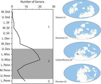
Eublastoid diversity has been commonly measured in terms of taxonomic (usually generic) abundances at given time intervals and represented by abundance plots or spindle diagrams (Waters Reference Waters, Paul and Smith1988, Reference Waters, McKerrow and Scotese1990; Fig. 1). The evolutionary history of eublastoids was described as occurring in three phases that are punctuated by diversification, radiation, and extinction (Waters Reference Waters, Paul and Smith1988). Through the lens of these phases, the biogeographic history and diversity of this clade was dissected and summarized (Waters Reference Waters, McKerrow and Scotese1990). These phases are redescribed below, updated with occurrence data from recent work.
Global occurrences of eublastoid taxa as represented in the Paleobiology Database separated out by geologic period. The number in parentheses corresponds to the evolutionary phases discussed in Waters (Reference Waters, Paul and Smith1988, Reference Waters, McKerrow and Scotese1990) and reevaluated here. Taxonomic diversity estimated using a smoothing three-term function to account for sampling bias as represented in Waters (Reference Waters, Paul and Smith1988).

The first phase marked the initial radiation of the group, previously described in the Ordovician, but now determined to be in the Silurian (Bauer et al. Reference Bauer, Waters and Sumrall2019). The first phase ends in the Devonian with a dramatic increase in lineage diversification and distribution across the globe followed by a subsequent decline at the end-Devonian extinction event. Macurda (Reference Macurda, Beaver and Moore1967) first summarized eublastoid distribution and noted that eublastoids reached a global distribution by the Devonian. In general, Devonian genera are restricted to a single continent, although some genera may have broad ranges within a continent (Macurda Reference Macurda, Beaver and Moore1967). At that time no known eublastoids had been found in the Late Devonian, which is now better sampled (e.g., Waters et al. Reference Waters, Maples, Lane, Marcus, Zhou-Ting, Lujun, Hong-Fei and Jin-Xing2003). Two collection trips to northwest Asia by Waters and others (described in Waters et al. Reference Waters, Maples, Lane, Marcus, Zhou-Ting, Lujun, Hong-Fei and Jin-Xing2003) quadrupled the known global Famennian pelmatozoan (stemmed echinoderms) diversity. Described as the Hongguleleng fauna, these echinoderms provide details on the transition from Devonian to Carboniferous pelmatozoans, particularly eublastoids and crinoids (Waters et al. Reference Waters, Maples, Lane, Marcus, Zhou-Ting, Lujun, Hong-Fei and Jin-Xing2003). The results of these sampling efforts have shifted the eublastoid extinction interval back to the Givetian/Frasnian boundary rather than the Frasnian/Famennian boundary (Waters et al. Reference Waters, Maples, Lane, Marcus, Zhou-Ting, Lujun, Hong-Fei and Jin-Xing2003).
The second phase of diversification is during the Carboniferous. The Mississippian has historically marked the peak of eublastoid taxonomic diversity in both North America and Western Europe (Macurda Reference Macurda, Beaver and Moore1967; Waters Reference Waters, Paul and Smith1988). However, the Mississippian peak in diversity is now rivaled by the Hongguleleng fauna in the Devonian (Waters et al. Reference Waters, Maples, Lane, Marcus, Zhou-Ting, Lujun, Hong-Fei and Jin-Xing2003). Several genera are found to have intercontinental range expansions during this time, including Pentremites, which is found to be cosmopolitan, with records ranging from Alaska to Colombia. The Pennsylvanian marks a sudden absence of eublastoids, with records from the western United States, Queensland, Australia, and Svalbard of only four genera. This may reflect a nonpreservational time in the geologic record and/or a bottleneck of diversity, but neither idea has been fully explored. Species richness and abundance are both lower during this phase, but in some environments, the eublastoids are the dominant echinoderm (e.g., the high-energy environment that deposited the Burlington Limestone; Waters Reference Waters, Paul and Smith1988). The end-Carboniferous (and end of phase 2) marks a sudden decline in diversity and abundance, with very few species recorded from the Pennsylvanian (Breimer and Macurda Reference Breimer and Macurda1972; Waters Reference Waters, McKerrow and Scotese1990).
The third and final phase of diversification is during the Permian and shows the resurgence of eublastoids in the Tethyan Seaway with the enigmatic Timor fauna and subsequent extinction at the end-Permian (Waters Reference Waters, McKerrow and Scotese1990). Timor and Western Australia provide a detailed record, with many species of both eublastoids and crinoids occurring at this time. Accompanying these seminal summary works were eublastoid distribution maps. Macurda (Reference Macurda, Beaver and Moore1967) provided maps with occurrences plotted on the modern continent arrangements, and this was subsequently updated by Waters (Reference Waters, McKerrow and Scotese1990), who used reconstructed paleocontinental configurations to plot occurrence data. Understanding past continental arrangements allows for a more accurate understanding of potential mechanisms of the distribution of eublastoid species (Fig. 1).
Materials and Methods
Occurrence and Area Data
Species occurrence data were required for each of the taxa included in the subsequent biogeographic analysis. Geographic data were compiled for each species using published literature and online biodiversity data aggregators, specifically iDigBio (www.idigbio.org) and the Paleobiology Database (PBDB; www.paleobiodb.org; Supplementary Table 1). Species temporal ranges were pulled directly from the PBDB, and if a species was not entered, the dates were used from the genus, if monospecific, or the formation it is found in, as the PBDB provides formation ages as well. Data from the data aggregators were verified against known publications.
The 52 eublastoid species used in this study were found in 19 depositional basins worldwide and through time. As this group persisted for over 150 Myr, there was much global change during this interval. To analyze the group as a whole rather than separate it out by time periods, these areas were combined into six major global basins that are broadly consistent throughout the Paleozoic. As the early Paleozoic is a dynamic time in terms of continental configuration, area delineation can be complex, as some basins migrate or do not persist throughout the entire time of interest. Combining into very broad areas was a first attempt to take these limitations into account. Future work should focus on increasing the number of areas and constraining different aspects of the tree topology. The six areas used in this study are: northern and eastern Laurussia (Laurentia + Baltica), western and eastern Gondwana, China, and Siberia (Fig. 2). From species occurrences, a presence–absence matrix was compiled as required for use in BioGeoBEARS.
Generalized geographic regions used for this analysis. Plate reconstruction is the Carboniferous generated by and modified from the Paleobiology Database.

Phylogenetic Analyses
Phylogenetic Inference
The phylogenetic framework for 52 species within Eublastoidea (Bauer Reference Bauer2018) was inferred through Bayesian estimation (see Supplementary File 1). The outgroup used for rooting the phylogeny is composed of two coronoid species, Cupulocorona gemmiformis and Stephanocrinus angulatus. The Nexus file was compiled in Mesquite (Maddison and Maddison Reference Maddison and Maddison2018) and executed in RevBayes (Höhna et al. Reference Höhna, Landis, Heath, Boussau, Lartillot, Moore, Huelsenbeck and Ronquist2016). The RevBayes simulation ran for 100,000 iterations. Resulting output files were visualized through Tracer (Rambaut et al. Reference Rambaut, Drummond, Xie, Baele and Suchard2018) and RStudio (R Studio Team 2015; R Core Team 2019). The maximum clade credibility (MCC) tree, which summarizes the results, was used for further analysis. The inferred phylogeny was then time calibrated for biogeographic analysis using the R package strapt (Bell and Lloyd Reference Bell and Lloyd2014). Equal length was used as a time-calibration method due to the requirements of subsequent biogeographic analysis of a minimum branch length greater than zero for the methods to be successfully employed.
Diversity and Ecology
The inferred phylogeny was used in several analyses. First, lineage diversity was estimated using paleotree (Bapst Reference Bapst2012). The time-calibrated MCC tree was then used to estimate clade diversity using phyloDiv. The function phyloDiv reconstructs the diversity given the phylogeny and dates incorporated into the time calibration.
Using the MCC tree, generalized sediment type was placed at the terminal nodes using phytools (Revell Reference Revell2012) to discern any evolutionary pattern to environmental preferences of these species. Data on sedimentology were culled from primary literature on the formations where these species were found and clarified with discussions by those who had been on the ground (J. A. Waters personal communication 2018; D. B. Macurda personal communication 2019). In earlier iterations, sediment type was subdivided into nine categories to accommodate more specific sediment types such as muddy and sandy carbonate, but the patterns were not apparent. To reduce the noise of overseparating groups, I simplified to the three sediment types: carbonate, siliciclastic, and mixed carbonate-siliciclastic. To assess phylogenetic signal among sediment types, Pagel's lambda (λ; Pagel Reference Pagel1999) and the K-statistic (Blomberg et al. Reference Blomberg, Garland and Ives2003) were employed using the phylosig function in the R package phytools (Revell Reference Revell2012). The p-value for the K-statistic was based on 1000 randomized iterations and Pagel's λ was based on the likelihood ratio test. Pagel's λ ranges from zero to one, where one is consistent with expectations under the Brownian motion model of evolution. A value of K equal to one for Blomberg's K indicates consistency with Brownian motion, similar to Pagel's λ. However, if K is greater than one, it is likely the traits of the sampled species are more similar to those of their ancestors than what would be expected given Brownian motion. If values are less than one or closer to zero, this indicates less or weak phylogenetic signal (Pagel Reference Pagel1999; Blomberg et al. Reference Blomberg, Garland and Ives2003).
Biogeographic Analyses
The biogeographic analyses require the inferred phylogeny to possess absolute temporal length of branches, meaning specific numeric dates. This is done by using the previously discussed time-calibrated phylogeny. Ancestral geographic ranges were inferred through probabilistic methods within the R package BioGeoBEARS (Matzke Reference Matzke2013; R Core Team 2019). Probabilistic methods, such as BioGeoBEARS, have been successfully employed by biogeographers primarily for the Mesozoic and Cenozoic eras but spanning plant, vertebrate, and invertebrate groups (e.g., Dantas et al. Reference Dantas, Weckstein, Bates, Krabbe, Cadena, Robbins, Valderrama and Aleixo2016; Poropat et al. Reference Poropat, Mannion, Upchurch, Hocknull, Kear, Kundrat, Tischler, Sloan, Sinapius, Elliott and Elliott2016; Toussaint and Balke Reference Toussaint and Balke2016). Analyses of all-fossil Paleozoic clades have been published more recently (Lam et al. Reference Lam, Stigall and Matzke2018; Congreve et al. Reference Congreve, Krug and Patzkowsky2019). In BioGeoBEARS, probabilistic models are fit to the data using maximum likelihood. These models allow the geographic ranges of species to evolve along branch lengths using range expansion and contraction processes that are controlled by the rate parameters d and e within each model, respectively. A species range can change during cladogenic events under several fixed models (DEC, DIVALIKE, BAYAREALIKE) that each include a modifier for founder-event speciation, or jump dispersal, through the parameter j. For a detailed discussion on the different models and incorporation of fossil datasets, see Lam et al. (Reference Lam, Stigall and Matzke2018).
Analyses were performed without dispersal constraints on directionality and timing of speciation events. The maximum range size (max_range_size) was set to three, which is the maximum number of areas occupied by any one species in the phylogeny to limit the size of state space available. The Akaike information criterion (AIC), corrected AIC (AICc), the difference between AICc and the best AICc (ΔAICc), and the AICc weight (ωi) as calculated from the log likelihood (lnL) values were used to compare model fit (Burnham and Anderson Reference Burnham and Anderson2002). Following O'Meara et al. (Reference O'Meara, Ané, Sanderson and Wainwright2006), AICc values were calculated using the number of taxa in the phylogeny as sample size. The best-fit model was selected from the aforementioned statistics and was then used to examine range size and speciation patterns through the study interval. Cladogenesis events were classified as being vicariance when a descendant occupied fewer areas than the direct ancestor or dispersal when the descendant occupied more or different areas than the direct ancestor. All scripts and associated files can be found in Supplementary File 2.
Results
Eublastoid Diversity and Ecology
The lineage diversity (Fig. 3) is broadly similar to the Waters (Reference Waters, Paul and Smith1988) curve (Fig. 1), but there are some notable differences. The initial eublastoid radiation in the Silurian was subsequently followed by a decline into the Devonian. There were then two pulses of diversity in the Devonian, one that becomes close to the peak Mississippian diversity. This was followed by a sudden decrease and plateau until the start of the Mississippian, where the peak diversity was recorded. This was short lived, and the second half of the Mississippian and entire Pennsylvanian depict a steady stepwise decline in diversity. The end low of the Pennsylvanian persists into the Permian with a small increase in diversity before the subsequent demise at the end-Permian extinction event.
Lineage diversity estimated through the paleotree R package. Evolutionary phases as outlined by Waters (Reference Waters, Paul and Smith1988, Reference Waters, McKerrow and Scotese1990) are noted on the diagram similar to Fig. 1. The peaks and troughs in diversity in phase 1 were previously depicted as a slow incline toward the Mississippian, rather than distinct events as they are estimated here.

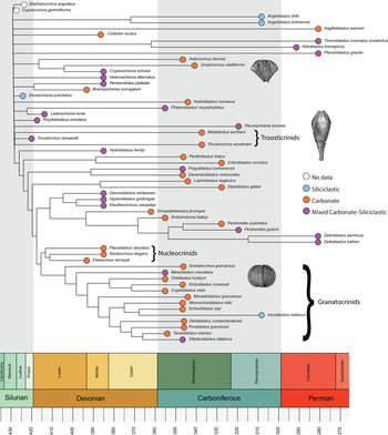
Carbonate, siliciclastic, and mixed sediment types were plotted at each terminal node to discern any evolutionary trends within the lithologic preferences of species. Mixed sediment includes carbonates with any amount or type of siliciclastic input. Phylogenetic signal was statistically assessed through lambda and K-statistics, where the input data were the resulting tree topology and the sediment data (carbonate, siliciclastic, or mixed). There are no obvious patterns displayed on the inferred phylogeny (Fig. 4), although there do appear to be some groupings of species preferring carbonate and/or mixed lithologies. The phyogenetic signal test found the K-statistic to be 0.128581 with a p-value of 0.034, and Pagel's lambda was 0.913475 with a p-value of 2.71081e-08. A K-statistic less than one suggests there is little signal within the dataset. Pagel's λ is less than one, although arguably close. The visual patterns will be discussed in the context of time and geographic region.
Generalized lithology for each species of eublastoid. Data were not included for the outgroup species. Phylogenetic signal statistics for Blomberg's K-statistic was 0.128581 with a p-value of <0.05, and Pagel's lambda was 0.913475 with a p-value of < 0.01. Siliciclastic is denoted by light blue, carbonate by orange, and mixed siliciclastic-carbonate by purple. Colors are easily distinguished in the online version of this paper. Species pictured near their locations on the tree: Orophocrinus stelliformis (USNM 41067), Troosticrinus reinwardti (CMC-IP 67717), and Globoblastus norwoodi (USNM S6800). Imaged by J. W. Atwood.

Biogeographic Analysis
The ΔAICc was used to select the best-fit model given the eublastoid dataset, which in this case was DIVALIKE + J, but DEC + J was very similar in estimated values (Table 1). DIVALIKE employs cladogenetic processes assumed by dispersal–vicariance analysis (DIVA; Ronquist Reference Ronquist1997) in a likelihood framework, where it allows single-area sympatry and any type of vicariance, but subset sympatry is excluded (Lam et al. Reference Lam, Stigall and Matzke2018). Conversely, DEC allows for single-area sympatry, subset sympatry, and narrow vicariance, where at cladogenesis the model assumes that at least one daughter only occupies one area (Lam et al. Reference Lam, Stigall and Matzke2018). The DIVALIKE + J was favored given the AICc weight (ωi) of 0.63 compared with 0.31 for DEC + J.
Comparison of model fits from the BioGeoBEARS analysis. lnL = log-likelihood values; AIC = Akaike information criterion; AICc = corrected AIC; ΔAICc = difference in AICc values compared with the best-fit model; ωi = AICc weight, the relative likelihood of a model; d = measure of dispersal rate along branches within the phylogeny; e = measure of extinction rate along branches within the phylogeny; j = measure of relative weight of jump dispersal.

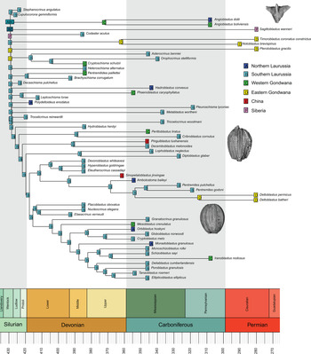
All three of the models with the + j parameter performed better than those without. The nodes within the phylogeny are signified by area letters, which represent the area(s) of the highest probability (Fig. 5) that the ancestors inhabited. A full breakdown of the ancestral probabilities can be found in Supplementary Figure 1. Under these parameters, terminal nodes that inhabit a single area will tend to favor + j models. This indicates jump dispersal will be favored when geographic ranges are coded on specimen location data rather than a species’ geographic range. This may lead to misleading results of clade origination or dominant mode of speciation within the clade. In the case of Eublastoidea, many species, and all included in this analysis, are endemic to a single geographic area, resulting in a similar confounding effect.
Results from the best-fit model of the BioGeoBEARS analysis: DIVALIKE + J. lnL (log-likelihood value) = −73.82; AICc (corrected Akaike information criterion) = 154.1.The nodes within the phylogeny are signified by area letters, signifying the areas of the highest probability that the ancestor inhabited these areas. The geographic areas are as follows: (A) northern Laurussia; (B) southern Laurussia; (C) western Gondwana; (D) eastern Gondwana; (E) China; (F) Siberia; and are the same as those delineated on Fig. 1. Geographic data for the species and the scripts for BioGeoBEARS can be found in Supplementary File 2. Gray and white alternating bands indicate the time periods. Species pictured near their locations on the tree: Pterotoblastus gracilis (USNM 248340), Lophoblastus neglectus (USNM S3726), and Elaeacrinus verneuilli (CMC-IP 35431). Imaged by J. W. Atwood.

Early on in the clade's history there are many possibilities for geographic origination of the eublastoids, indicated by the multiple inhabited areas at the base of the clade (Fig. 5; Supplementary Fig. 1). The oldest ancestral nodes were estimated to inhabit all geographic areas, with the exception of China. The backbone of the phylogeny is rooted in the Silurian, and there is more clarity in the probable ancestral areas, with two possible areas being southern Laurussia and eastern Gondwana. During the Devonian, the majority of ancestral ranges are restricted to southern Laurussia with minor probability split between northern and southern Laurussia (Supplementary Fig. 1). In the Carboniferous, all but two ancestral nodes are in southern Laurussia, with the other two being eastern Gondwana.
Speciation Patterns
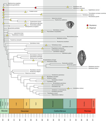
Speciation across the inferred biogeographic patterns includes dispersal, vicariance, and sympatric speciation (Fig. 6). This inferred phylogeny shows more than 10 times as many dispersal events (n = 23) as vicariance events (n = 2), with the majority of the nodes representing sympatric speciation within the same geographic area (Fig. 7). These results suggest vicariance events occur only in the Silurian and Devonian from different areas to eastern Gondwana.
Modes of speciation in each major geologic interval given the BioGeoBEARS results. Speciation events were designated at internal nodes and terminal nodes for these counts. As with other fossil clade studies, dispersal is greater than vicariance events, but here sympatric speciation is constantly dominant. This has been attributed to the simplification of areas causing a high degree of within-area speciation.

Speciation modes of vicariance (descendant in fewer areas than ancestor) or dispersal (descendant in more or different areas than ancestor) mapped onto the inferred phylogeny. Nodes with no shape are inferred to be sympatric speciation events. Speciation events that occur along a branch are indicated at the first occurrence record of that species. Gray and white alternating bands indicate the time periods. Species pictured near their locations on the tree: Brachyschisma corrugatum (USNM 387783) and Ambolostoma baileyi (USNM 111726). Imaged by J. W. Atwood.

Discussion
Clade Diversity and Evolutionary Phases
Eublastoid diversity estimated through the lineage richnesses function in paleotree, matches previous estimates from strictly taxonomic datasets of eublastoid diversity. Previous diversity curves suggest the Mississippian as the high point in eublastoid diversity (Waters Reference Waters, Paul and Smith1988; Fig. 1), which it certainly is in terms of abundance and species present. This new estimation (Fig. 3) takes the evolutionary history of the clade into account, and it suggests a comparable peak in the Devonian. Waters et al. (Reference Waters, Maples, Lane, Marcus, Zhou-Ting, Lujun, Hong-Fei and Jin-Xing2003) have shown that concerted sampling efforts in remote areas of the world can drastically alter our understanding of eublastoid and echinoderm diversity. This expands to Echinodermata as a whole, with recent global sampling efforts altering our understanding of the early evolution of this diverse clade (see Sumrall et al. Reference Sumrall, Deline, Colmenar, Sheffield, Zamora, Zamora and Rábano2015; Zamora et al. Reference Zamora, Sumrall, Zhu and Lefebvre2017; Sumrall and Zamora Reference Sumrall and Zamora2018). Other biases likely influence our understanding of echinoderm diversity as well, particularly preservational bias in the end-Carboniferous, where there are very few recorded species (Macurda Reference Macurda, Beaver and Moore1967).
Incorporating parameters such as the evolutionary history to influence the understanding of the clade's diversity can help mitigate some of the biases that are inherent in taxonomic occurrence data. The diversity curve exhibits similarities to Waters (Reference Waters, Paul and Smith1988) but is much higher resolution. The most notable differences are the dynamic nature of the curve in phase 1, Silurian and Devonian periods. In Waters (Reference Waters, Paul and Smith1988), the curve indicates a steady increase to the peak diversity in the Mississippian. The lineage diversity estimated here reveals really interesting dynamics that would be less clear from taxonomic counts alone. The diversification of the Hongguleleng fauna is likely the high peak seen in the Devonian. The large plateau at the end of the Devonian is dramatic and could be due to lack of origination rather than extinction of these groups (Stigall et al. Reference Stigall, Bauer, Lam and Wright2017).
Paleoecology and Lithologic Preference
Results from the eublastoid lithologic preference visual mapping (Fig. 4) and phylogenetic signal statistics are inconclusive. Because this estimated phylogeny is limited in scope, containing 52 of more than 200 described species, it is subject to change as more taxa are added to the analysis. The phylogenetic signal statistics suggest a weak signal for substrate preference; however, the K-statistic was quite close to one. This indicates that more work needs to be done exploring lithology as it relates to the Eublastoidea.
Geographic and Temporal Distribution
There are very few described Silurian species, the two included in this analysis are found in southern Laurentia and prefer different lithologies. The first radiation of eublastoid diversity occurred during the Devonian, and there appears to be a preference toward mixed carbonate-siliciclastic lithology (n = 9), with less carbonate preference (n = 5), and there are no species with siliclastic preference. The transition into the Mississippian suggests a shift from mixed carbonate-siliclastic (n = 6) preference in the Devonian to a carbonate-dominant preference (n = 22). This supports previous work that outlined the Mississippian as the peak diversity of eublastoids on the high-energy carbonate platforms (Waters Reference Waters, Paul and Smith1988, Reference Waters, McKerrow and Scotese1990). Three species, all occurring in the Pennsylvanian, are recovered from siliciclastic environments. The Permian depicts a shift back to a preference of mixed carbonate-siliciclastic lithology (n = 5) compared with one species that prefers carbonate lithology. A caveat is that the five Permian taxa that prefer the mixed lithology are all from the same area, Timor or eastern Gondwana in the biogeographic analysis.
Evolutionary Implications
There are several patterns that arise and other noteworthy observations when considering the evolution of subclades in Eublastoidea. There appears to be conservativism in lithologic preference within the well-established and temporally restricted nucleocrinid clade (Nucleocrinus, Elaeacrinus, Placoblastus), with all genera preferring carbonate lithology (Fig. 4), whereas the troosticrinids (Troosticrinus, Tricoelocrinus, Metablastus) show a shift from mixed carbonate-siliciclastic lithology in the Devonian to carbonate in the Mississippian. The large granatocrinid clade (n = 13) primarily prefers carbonate lithology (n = 10) with few taxa preferring a mixed environment (n = 2) and one preferring siliciclastic. Given the coarse nature of the biogeographic areas, it is difficult to confidently make statements regarding the relationship among speciation, geography, and the inferred tree topology.
Biogeographic and Speciation Patterns
The results herein largely match the summary conducted by Waters (Reference Waters, Paul and Smith1988, Reference Waters, McKerrow and Scotese1990), provide a quantitative framework to assess the patterns found, and consider ancestral species ranges. Waters (Reference Waters, McKerrow and Scotese1990) concluded that eublastoids seemingly originated in North America and were largely restricted to Laurussia with subsequent radiations and dispersals across the globe. The most basal nodes on the phylogeny indicate probabilities of an ancestor inhabiting multiple areas, meaning I cannot say with certainty where eublastoids originated (see Supplementary Fig. 1). However, the majority of the clade has ancestral roots in Laurussia.
The majority of recovered cladogenetic events were sympatric speciation or no change from the ancestral range (Fig. 6). This is likely due to the lumping of areas in this study, particularly the southern Laurussia region, where there are upward of 11 intracratonic basins throughout the Paleozoic. BioGeoBEARS has to exponentiate a matrix, so if there are too many possible states (the number of different possible geographic ranges), the computing power is often not enough, and the first likelihood will never be produced. This can be mitigated to a degree by forcing a maximum range size (max_range_size) for each species (Matzke Reference Matzke2013). Additionally, basins do not continually persist over extremely long timescales, a factor that complicates the structure of the analysis.
The Silurian was a time of high separation between landmasses, until the end, when the Iapetus Ocean closed and Avalonia–Baltica collided with Laurentia in the Caledonide orogeny to create Laurussia (Torsvik and Cocks Reference Torsvik and Cocks2016a). As is common with isolated landmasses, the few species occurrences during the Silurian were restricted to Laurussia. At the start of the Devonian, the Rheic Ocean was at its widest extent between Laurussia and Gondwana, and it narrowed as the period progressed (Torsvik and Cocks Reference Torsvik and Cocks2016b). During this period there were several notable eublastoid dispersal events, from Laurussia to western Gondwana and China (Fig. 7). As the Rheic Ocean shrunk, the connectivity between the fauna of Laurussia and western Gondwana increased (Torsvik and Cocks Reference Torsvik and Cocks2016b) and was represented by a notable Spanish eublastoid fauna. The Chinese dispersal event of Sinopetaloblastus marked a long-distance dispersal event. As the Rheic closed, the Paleotethys became larger (Torsvik and Cocks Reference Torsvik and Cocks2016b), which would alter ocean circulation and local gyres, promoting the transport of larval-stage individuals to different regions. Not all of the Asian fauna are represented in this inferred phylogeny, so this result may change with the incorporation of more species from this time. Across the clade's history, there were seemingly multiple migrations to western Gondwana from Laurussia (Fig. 7).
The apex of eublastoid diversity was in the Mississippian, with most lineages established in the Devonian. There were two dispersal events to eastern Gondwana, one early in the Carboniferous and the other later, both through the Paleotethys Ocean. The Rheic Ocean underwent final closure in the Carboniferous (Torsvik and Cocks Reference Torsvik and Cocks2016c), and this likely strengthened circulation within the Paleotethys. Little is known about eublastoids from the Pennsylvanian, with only a few occurrences documented. The resurgence fauna in Timor (eastern Gondwana) has been well studied, but the biogeographic origin and affinities to other eublastoids is still unclear. Here I find that there were at least two lineage migrations in the Carboniferous from southern Laurussia to Timor (Fig. 7). The Permian marks the final assemblage of Pangea (Torsvik and Cocks Reference Torsvik and Cocks2016d), and many of the eublastoid species have gone extinct by this time. The one Siberian species evolved from an ancestor that dispersed from either Laurussia or western Gondwana but the estimated probabilities for areas here were low (see Supplementary Fig. 1).
Results from this study align with other fossil estimations of biogeographic patterns. Previous work using BioGeoBEARS has determined that models that incorporate long-distance dispersal events perform better. Lam et al. (Reference Lam, Stigall and Matzke2018) examined 10 extinct clades of Late Ordovician brachiopod and trilobite taxa, with their results suggesting 70% of the clades performed better with models that included jump dispersal. Similarly, Congreve et al. (Reference Congreve, Krug and Patzkowsky2019) examined a large Ordovician brachiopod clade and also had a best-fit model that included the + j parameter. Findings of these previous studies, combined with the results of this study, provide further support that long-distance founder-event speciation was a major mode of speciation for Paleozoic clades.
Summary and Future Work
This work represents the first quantitative biogeographic study of the Eublastoidea, a clade persisting for over 150 Myr, spanning four periods in the Paleozoic. Results suggest Eublastoidea was largely a Laurentian clade, though still with unclear geographic origins. The broad geographic areas defined here are a first approximation to determine the speciation type and major dispersal paths for the Eublastoidea within a rigorous statistical framework. To explore the geographic origins of the clade and undertake a detailed examination of speciation patterns, the geographic areas will need to be more finely defined in future analyses. Future work will revisit all known areas and use different means to constrain the tree topology to run additional analyses.
Estimating clade diversity with incorporation of phylogeny and time provides a more detailed understanding than previous analyses on taxonomic counts. This diversity curve also incorporates some of the newly discovered species but not all. The continued effort to expand the phylogeny will increase our understanding of clade diversity as well. Exploring the lithologic data alongside the phylogeny has not previously been done for eublastoid taxa, and the present results are inconclusive, but interesting patterns arise when examining ordinal-level groupings and should be resolved with increased taxa in the estimated phylogeny. Increasing resolution of the geographic areas will also provide an avenue for more detailed paleoecology to be unraveled. As it currently stands, the resolution is too poor to make supported statements.
As mentioned previously, the Eublastoidea has upward of 200 described species. The phylogenetic and taxonomic details must be evaluated before we can continue to examine this robust clade. Work to redefine and redescribe various subgroups of eublastoids is currently underway and will undoubtedly build upon the results presented here.
Other biogeographic studies in the Paleozoic have focused on specific intervals of time such as the Ordovician biotic crisis (Lam et al. Reference Lam, Stigall and Matzke2018; Congreve et al. Reference Congreve, Krug and Patzkowsky2019) or the great Ordovician biodiversification event (Lam et al. Reference Lam, Sheffield and Matzke2020). With such a long-lived clade and coarse resolution of geographic areas, it is difficult to determine key moments that may have affected life on Earth. There are many Paleozoic clades that can contribute to this understanding, some with published inferred phylogenies. Future work on this project will provide a comprehensive examination into each of the time periods by examining the speciation of the clade in the context of isotopic excursions, sea-level fluctuations, biotic crises, and plate tectonic movements.
Acknowledgments
Appreciation to both M. Nohejlová and C. Congreve for thoughtful comments that enhanced the quality of this project. Special thanks to J. Lamsdell and C. Congreve for the productive and interesting session at the 2018 Geological Society of America meeting. I would like to thank A. R. Lam, M. R. Limbeck, and S. L. Sheffield for their thoughtful comments on earlier versions of this article. Fruitful discussions with J. A. Waters and D. B. Macurda provided the foundation and continuation of this project. For part of this project I was funded by the Thompson Earth Systems Institute and the FOSSIL Project (NSF DRL-1322725) at the University of Florida.