Instability growth and fragment formation in air assisted atomization

G. Singh; A. Kourmatzis; A. Gutteridge; A. R. Masri

doi:10.1017/jfm.2020.179

Instability growth and fragment formation in air assisted atomization

Published online by Cambridge University Press: 06 April 2020

A. Gutteridge and

G. Singh: Affiliation:
School of Aerospace, Mechanical and Mechatronic Engineering, University of Sydney, NSW2006, Australia
A. Kourmatzis*: Affiliation:
School of Aerospace, Mechanical and Mechatronic Engineering, University of Sydney, NSW2006, Australia
A. Gutteridge: Affiliation:
School of Aerospace, Mechanical and Mechatronic Engineering, University of Sydney, NSW2006, Australia
A. R. Masri: Affiliation:
School of Aerospace, Mechanical and Mechatronic Engineering, University of Sydney, NSW2006, Australia
*: † Email address for correspondence: agisilaos.kourmatzis@sydney.edu.au

Article contents

Abstract
Introduction
Experimental setup
Development of surface instabilities
Formation of liquid fragments
Comparison with theoretical models
Conclusion
References

Rights & Permissions

Abstract

This paper reports an extensive study on the morphology of wave formation on the liquid core of atomizing sprays. The gas velocity, liquid jet velocity and liquid jet size are varied for two different fuels resulting in a range of liquid jet Reynolds numbers, aerodynamic Weber numbers and mass flux ratios. The liquid jet Reynolds number can be used to predict the initiation of jet instabilities, with coaxial air-flow velocity controlling their subsequent growth. A categorization of waves on the surface of the liquid according to their amplitude and wavelength has enabled (i) the identification of a threshold that leads to breakup, and (ii) the isolation of waves that lead to ligament formation from waves that result in droplets. The probability distribution of measured wavelength reasonably matches that of the ligament length, with no requirement for empirical constants. This confirms a direct link between interfacial instabilities and ligament formation in air assisted primary atomization.

JFM classification

Drops and Bubbles: Aerosols/atomization

Information

Type: JFM Papers
Information: Journal of Fluid Mechanics , Volume 892 , 10 June 2020, A29
DOI: https://doi.org/10.1017/jfm.2020.179 [Opens in a new window]
Copyright: © The Author(s), 2020. Published by Cambridge University Press

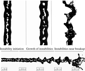
1 Introduction

In an air-blast atomizer, breakup is caused by the transfer of kinetic energy from the high-speed gas to the liquid jet (Lefebvre Reference Lefebvre1980; Lin & Reitz Reference Lin and Reitz1998). The breakup morphology and its dependence on non-dimensional parameters has been studied extensively both experimentally (Faeth Reference Faeth1996; Lasheras, Villermaux & Hopfinger Reference Lasheras, Villermaux and Hopfinger1998; Varga, Lasheras & Hopfinger Reference Varga, Lasheras and Hopfinger2003; Marmottant & Villermaux Reference Marmottant and Villermaux2004) and numerically (Shinjo & Umemura Reference Shinjo and Umemura2010; Umemura Reference Umemura2011). Farago & Chigier (Reference Farago and Chigier1992) have classified breakup regimes for a coaxial air-blast atomizer in a Weber number and jet Reynolds number space. For low-Weber-number sprays ($We<15$), the breakup is governed by axisymmetric instabilities, and follows a Rayleigh breakup mode, which results in droplets of a size proportional to the liquid jet diameter $(d_{drop}\sim 2d_{jet})$ (Farago & Chigier Reference Farago and Chigier1992; Faeth, Hsiang & Wu Reference Faeth, Hsiang and Wu1995; Faeth Reference Faeth1996; Dumouchel Reference Dumouchel2008). Shear driven Kelvin–Helmholtz instabilities govern jet breakup for high-Weber-number sprays ($We>25$) (Farago & Chigier Reference Farago and Chigier1992; Dumouchel Reference Dumouchel2008).

A thorough description of the dynamics of interfacial instabilities is central to the prediction of fragment formation. Surface instabilities initially form on the liquid jet surface and interact with the surrounding high-speed gas. These instabilities, named here as primary instabilities, grow in magnitude while moving downstream, and eventually lead to jet breakup. Recently there has been significant work in studying surface instabilities by employing linear stability analysis, and mixing layer experiments, where a liquid surface is destabilised by parallel flowing air (Villermaux Reference Villermaux1998; Gordillo, Perez-Saborid & Ganan-Calvo Reference Gordillo, Perez-Saborid and Ganan-Calvo2001; Matas, Marty & Cartellier Reference Matas, Marty and Cartellier2011; Fuster et al. Reference Fuster, Matas, Marty, Popinet, Hoepffner, Cartellier and Zaleski2013; Matas Reference Matas2015). It is reported that the frequency of the instabilities does not change spatially; however, the velocity profile of the jet and the velocity deficit at the interface significantly affect the jet instabilities (Matas et al. Reference Matas, Marty and Cartellier2011). Work by Gordillo et al. (Reference Gordillo, Perez-Saborid and Ganan-Calvo2001) examined the effect of viscosity for constant Weber number and momentum flux ratios. Similarly, Matas (Reference Matas2015), Otto, Rossi & Boeck (Reference Otto, Rossi and Boeck2013), and Fuster et al. (Reference Fuster, Matas, Marty, Popinet, Hoepffner, Cartellier and Zaleski2013) compared the inviscid and viscous instability mechanism, and determined that the inclusion of a viscosity term in linear stability analysis can have an impact on frequency and growth rate prediction. Matas, Delon & Cartellier (Reference Matas, Delon and Cartellier2018) extended the instability analysis to coaxial atomizers and reported scaling laws governing the jet instability, where it was found that the frequency of the instability is a function of gas velocity, liquid velocity and nozzle-length scales. Whilst progress is significant, the majority of previous work on surface instabilities has been focused on jets having momentum ratio $(M>5)$, and direct statistical links between instability formation and downstream fragment formation remain scarce in the literature.

The work of Marmottant & Villermaux (Reference Marmottant and Villermaux2004) is arguably one of the most extensive contributions describing the role of instabilities in fragment formation. However, a detailed statistical analysis had not been conducted at the time, with much of the description of the role of jet instabilities being based on either analytical calculations or still photographs. This work was extended by Varga et al. (Reference Varga, Lasheras and Hopfinger2003) who reported a relation between initial primary instabilities and Rayleigh–Taylor instabilities which occur at the interface of two accelerating fluids with different densities. When a liquid fragment is suddenly exposed to a high-speed gas stream this instability forms on the surface and, if sufficiently large, leads to fragment breakup (Varga et al. Reference Varga, Lasheras and Hopfinger2003; Marmottant & Villermaux Reference Marmottant and Villermaux2004). Varga et al. (Reference Varga, Lasheras and Hopfinger2003) developed a correlation between the primary and Rayleigh–Taylor instabilities and reported that droplet formation is dictated by the latter. Kourmatzis & Masri (Reference Kourmatzis and Masri2015) also suggested this to be likely at both high and low levels of gas-phase turbulence intensity while also reporting that ligament formation is, at least on average, governed by the primary instability.

Umemura (Reference Umemura2011) carried out work enabling the categorization of waves into two types of modes for fragment breakup: a long wave mode and short wave mode, with the latter being dominant near the jet tip and governing droplet breakup. Similarly, earlier work by Eroglu, Chigier & Farago (Reference Eroglu, Chigier and Farago1991) measured the wave frequency of liquid jet undulations and was able to deduce two types of wavelengths for low and high liquid velocities (low and high $Re_{jet}$). They reported a sinuous wave for low liquid velocity jets and a dilated wave for jets having high liquid velocity. Mayer & Branam (Reference Mayer and Branam2004) reported that the liquid flow, driven by $Re_{jet}$, controls the initiation of the surface instabilities in coaxial atomizers. In general however, thorough investigation of the role of the liquid jet velocity and Reynolds number on initiation of instabilities has been sparse.

Entrainment in coaxial atomizers is also a process that can govern jet instabilities and the atomization mechanism and can be non-dimensionally related to the mass flux ratio (Engelbert et al. Reference Engelbert, Hardalupas, Whitelaw and Launder1995; Faeth et al. Reference Faeth, Hsiang and Wu1995; Lasheras & Hopfinger Reference Lasheras and Hopfinger2000; Dumouchel Reference Dumouchel2008; Shinjo & Umemura Reference Shinjo and Umemura2010; Kourmatzis & Masri Reference Kourmatzis and Masri2015; Kourmatzis, Lowe & Masri Reference Kourmatzis, Lowe and Masri2016). Lasheras et al. (Reference Lasheras, Villermaux and Hopfinger1998) investigated the breakup of a round liquid jet and reported the effect of entrainment on the length of the liquid column before its breakup. Kourmatzis & Masri (Reference Kourmatzis and Masri2015) analysed the effect of turbulence intensity and the role of gas phase fluctuations on the breakup process. They defined a turbulent Weber number ($We^{\prime }$) using velocity fluctuations, and reported the effect of entrainment in terms of $We^{\prime }$, mass flux ratio and mean shear at the liquid–air interface.

Regardless of the non-dimensional space and context of previous studies, the literature has consistently suggested that Rayleigh–Taylor instabilities and Kelvin–Helmholtz instabilities are partly dictating the atomization process (Lasheras et al. Reference Lasheras, Villermaux and Hopfinger1998; Lasheras & Hopfinger Reference Lasheras and Hopfinger2000; Varga et al. Reference Varga, Lasheras and Hopfinger2003; Marmottant & Villermaux Reference Marmottant and Villermaux2004; Dumouchel Reference Dumouchel2008; Shinjo & Umemura Reference Shinjo and Umemura2010; Kourmatzis & Masri Reference Kourmatzis and Masri2015). However, direct measurements and statistical analysis of instability wavelengths and amplitudes on the liquid jet surface with modern image processing techniques have yet to be presented. Time-resolved measurement of all instabilities on the jet surface is necessary to enable the development of physical correlations between instability formation and fragment or droplet formation. Such information would not only aid in our fundamental understanding of what generates the droplet size and ligament size distributions, but will also enable new analytical models whilst in parallel providing a detailed experimental data set for the future development of numerical predictive tools for atomization.

This contribution presents measurements of near-field jet instabilities and their relation to fragment formation using multi-angle high-speed imaging employing thousands of images for accurate statistical analysis. Both the wavelength and amplitude of the surface instabilities are directly measured in an effort to provide extensive detailed quantitative studies which link the statistical distributions of instability sizes on the liquid jet to fragment distributions downstream, whilst comparing to established analytical scalings. A range of sprays using three liquid jet sizes and two fuels (acetone and ethanol) are investigated with the liquid mass flow rate and gas phase velocity also altered to cover a wide spectrum of non-dimensional numbers, including a variation over the Weber number, jet Reynolds number, gas Reynolds number and mass flux ratio. These non-dimensional numbers are defined in § 2.

The paper will begin with a description of the diagnostic and image processing methodologies employed to measure the wavelength and amplitude of the jet instabilities. This is followed by a discussion of the dynamics of jet instabilities in terms of initiation, growth and categorization according to non-dimensional groups. Relationships between the jet instabilities and mechanisms governing the fragment size will then be presented. The final section will compare the experimental findings of this work with data and theoretical models reported in the literature by Varga et al. (Reference Varga, Lasheras and Hopfinger2003), Marmottant & Villermaux (Reference Marmottant and Villermaux2004), Umemura (Reference Umemura2011) and Kourmatzis & Masri (Reference Kourmatzis and Masri2015).

2 Experimental setup

The experimental setup is illustrated in figure 1. The spraying system consists of a standard coaxial air-blast atomizer (Sydney University Needle Burner) installed in a wind tunnel of cross-section $180\times 180~\text{mm}$ to minimise any influence from the surrounding laboratory air. The wind tunnel generates a co-flow of air with a mean axial velocity of $5~\text{m}~\text{s}^{-1}$ and a turbulence intensity of 8 %. The burner is a typical air-blast burner, which is widely reported in the literature (Kourmatzis, Pham & Masri Reference Kourmatzis, Pham and Masri2017; Lowe, Kourmatzis & Masri Reference Lowe, Kourmatzis and Masri2017) so only the important features of the atomizer are discussed here. The atomizer is equipped with an adjustable needle where its distance from the exit can be varied to facilitate generation of a range of sprays – a traditional coaxial air-blast boundary is produced when the needle is flush with the injector exit and a more dilute spray is gradually produced as the needle is recessed upstream from the injector exit plane. The air-blast diameter ($D$) and pilot annulus ($D_{p}$) are kept constant at $D=10~\text{mm}$ and $D_{p}=25~\text{mm}$, respectively. The distance between the needle top and the air-blast tube exit is defined as the recess length ($Lr$). For this investigation, the needle is kept flush with the burner exit $(Lr=0)$ for all cases.

Figure 1.

Illustration of experimental setup. Inset image shows the cut section of the injector.

The imaging set-up consists of two high-speed cameras (LaVision HSS6) each coupled with a long-distance microscope ($QM100$) of $45~\unicode[STIX]{x03BC}\text{m}$ depth of field. The two cameras are mounted perpendicular to each other to facilitate two views of the spray. These will be used to obtain information regarding the small perturbations on the jet surface, which are visible from one view, but are sometimes not visible from a single view due to occlusion. A high-speed laser Nd-YAG laser (Edgewave) is used as a light source for the imaging system. The laser beam from the high-speed laser is divided into two streams of equal intensity, using a 50–50 beam splitter; one beam for each camera. Using suitable optics, the beams are guided towards optical diffusers placed near the measurement volume. The long-distance microscope facilitates imaging in the near-field region of the spray, which is illuminated by diffused laser light produced from the high-speed laser. Davis (LaVision) imaging software is used to control the data collection. To investigate jet instabilities and spray formation in the downstream region of the spray, the images are captured at several axial locations. For each location, two thousand images are captured at a repetition rate of 5 kHz. The size of each image is $768\times 768$ pixels with a spatial resolution of $4.5~\unicode[STIX]{x03BC}\text{m}~\text{pixel}^{-1}$. This results in an image size of $3.46\times 3.46~\text{mm}$.

Table 1.

Size specification for needles: N17, N19 and N21.

Table 2.

Case specifications with relevant non-dimensional numbers for needle N21. Here, $Q_{liquid}~(\text{gm}~\text{min}^{-1})$ is the liquid loading, $U_{gas}~(\text{m}~\text{s}^{-1})$ is the air-blast speed, $U_{liquid}~(\text{m}~\text{s}^{-1})$ is the liquid jet velocity, $Re_{jet}$ is the Reynolds number of the liquid jet, $Re_{air}$ is the Reynolds number of the air-blast and $We$ is the aerodynamic Weber number. All non-dimensional numbers are calculated at the burner exit plane.

To study the effect of liquid properties and non-dimensional parameters on instability formation and their subsequent influence on the downstream spray structure, several cases are investigated by employing three liquid needles: N17, N19 and N21, with size specifications as described in table 1. Two liquids, acetone and ethanol, are used to generate sprays to cover a range of non-dimensional numbers. These are detailed for each needle size in tables 2, 3 and 4. Prefixes ‘A’ and ‘E’ in the case names refer to acetone and ethanol, respectively. For four cases (case 11, case 12, case 13 and case 14), the liquid loading and slip velocity are kept the same to have both a common Weber number and jet Reynolds number ($Re_{jet}$) for all three needles and both liquids. Three cases (case 15, case 16 and case 17) are varied in liquid loading and air-blast to cover a range of mass flux ratios, $Re_{jet}$ and Weber number. Overall, the cases investigated here cover variations in all the important non-dimensional numbers, defined in (2.1)–(2.5), where $m$ is the mass flux ratio and $M$, as defined in Lasheras et al. (Reference Lasheras, Villermaux and Hopfinger1998), is the momentum flux ratio per unit volume:

(2.1)

$$\begin{eqnarray}\displaystyle & \displaystyle Re_{air}=\frac{U_{gas}D_{gas}}{v_{gas}}, & \displaystyle\end{eqnarray}$$

(2.2)

$$\begin{eqnarray}\displaystyle & \displaystyle Re_{jet}=\frac{U_{liquid}D_{liquid}}{v_{liquid}}, & \displaystyle\end{eqnarray}$$

(2.3)

$$\begin{eqnarray}\displaystyle & \displaystyle We=\frac{\unicode[STIX]{x1D70C}_{gas}(U_{gas}-U_{liquid})^{2}D_{liquid}}{\unicode[STIX]{x1D70E}}, & \displaystyle\end{eqnarray}$$

(2.4)

$$\begin{eqnarray}\displaystyle & \displaystyle m=\frac{\unicode[STIX]{x1D70C}_{liquid}U_{liquid}Area_{jet}}{\unicode[STIX]{x1D70C}_{gas}U_{gas}Area_{air-blast}}, & \displaystyle\end{eqnarray}$$

(2.5)

$$\begin{eqnarray}\displaystyle & \displaystyle M=\frac{\unicode[STIX]{x1D70C}_{gas}U_{gas}^{2}}{\unicode[STIX]{x1D70C}_{liquid}U_{liquid}^{2}}. & \displaystyle\end{eqnarray}$$

Table 3.

Case specifications with relevant non-dimensional numbers for needle N19.

Table 4.

Case specifications with relevant non-dimensional numbers for needle N17.

2.1 Wave extraction methodology

The spray images are processed using a MATLAB code developed in-house. To separate the liquid object from the background, the images are binarized using a well-validated threshold-based methodology presented elsewhere (Kourmatzis, Pham & Masri Reference Kourmatzis, Pham and Masri2015). The threshold intensity is selected carefully to minimise uncertainties regarding droplet merging and out-of-focus objects. A maximum error of 10 % in object size is expected with the detailed image binarization adapted here along with the detailed calibration technique discussed elsewhere (Kourmatzis et al. Reference Kourmatzis, Pham and Masri2015, Reference Kourmatzis, Pham and Masri2017; Lowe et al. Reference Lowe, Kourmatzis and Masri2017).

Figure 2.

Definition of measured wavelength and amplitude of the instabilities. Panel (a) shows the actual jet and panel (b) shows a processed image of the jet. The left image is captured at the burner exit and its size is approximately equal to $3.5\times 3.5~\text{mm}$.

To measure the wavelength of the jet instabilities from the binarized image, the jet boundary is extracted to identify the waves and their peaks. The wavelength is measured as the distance between two subsequent peaks, as shown in figure 2. The velocity of the wave is calculated by tracking the wave peaks in two subsequent time frames (usually captured within $30~\unicode[STIX]{x03BC}\text{s}$, using PIV mode). The peaks and crests in a boundary are identified on the basis of the fact that the first derivative of the boundary will be zero $(\text{d}y/\text{d}x=0)$ at these points. A smoothing filter of 5 pixels is applied to the extracted boundary to clearly identify the peak points. Application of a single pixel threshold for binarization and a Gaussian image intensity profile can result in false peaks of very low amplitude. Therefore, various limiting criteria are applied to minimise error in wave detection. First, a linear curve fitting model is applied on the extracted wave to remove peaks that form a line using an $R^{2}$ limit of 0.95 (see appendix A for further details). Owing to use of a smoothing filter of 5 pixels, which corresponds to ${\sim}20~\unicode[STIX]{x03BC}\text{m}$, a limiting value of 0.02 mm for amplitude along with a limiting value of 0.05 mm for wavelength is applied to avoid the influence of background noise. The limiting value of 0.05 mm for the wavelength makes this technique only suitable for the measurement of interfacial instabilities formed on the primary liquid jet core and larger ligaments, not on subsequent fragments formed downstream. In general, the instabilities formed on downstream liquid fragments are very small and cannot be resolved here; hence, only surface instabilities on the liquid jet surface are discussed in this contribution. Further details on the processing technique are provided in appendix A. For each location, 2000 images are processed to measure the wavelength and amplitude of the instabilities, and more than 2500 wavelengths are measured and used for statistical analysis. This number of images results in an acquisition time significantly longer than the characteristic breakup time scale for the range of Weber numbers covered here (Kourmatzis & Masri Reference Kourmatzis and Masri2015).

3 Development of surface instabilities

In this section we present results on the initiation and growth of surface instabilities. Firstly, we focus on the global characteristics of wavelength followed by a description of the parameters governing the instabilities at the initiation point and near to the jet breakup location. There will be a focus on the description of two types of instabilities: primary instabilities ($\unicode[STIX]{x1D706}_{p}$) and secondary instabilities ($\unicode[STIX]{x1D706}_{\bot }$), which will be defined in § 3.3.

Figure 3.

The probability density distribution of wavelength of all the surface instabilities observed on the liquid jet, from burner exit to jet breakup, for several cases of needle N19 for acetone and ethanol. Cases 12, 13 and 14 have the same liquid loading but different gas velocities. Cases 15 and 17 have the same Weber number but different $Re_{jet}$. Subscript ‘T’ denotes a turbulent case and subscript ‘L’ denotes a laminar case.

3.1 Global nature of surface instabilities

In figure 3 we show the probability density distribution of wavelength of all the surface instabilities observed on the jet surface, from atomizer exit until jet breakup, for several cases of acetone and ethanol sprays of needle N19. The probability density distribution of wavelength of instabilities for five cases of both acetone and ethanol sprays are compared. Cases 12, 13 and 14 have different gas velocities (presented in terms of $We$) but the same liquid loading which results in $Re_{jet}=4180$ and $1170$ for acetone and ethanol sprays, respectively. We note that, for constant $Re_{jet}$, the wavelength distribution shifts towards a shorter wavelength with increasing Weber number. This is expected because with an increase in Weber number the higher air-blast speed enhances the influence of aerodynamic forces on the liquid jet, and amplifies surface perturbations which result in instabilities of high amplitude and small wavelength. The reader should note that, for these cases, the increase in Weber number is generally driven by an increase in air-blast velocity. Cases 15 and 17 have the same Weber number but different $Re_{jet}$. For case 15, the liquid jet is laminar and, for case 17, it is turbulent. In this paper, a nominal transition from laminar to turbulent flows is assumed at about $Re\approx 2300$. It is interesting to note that the instability wavelength for the laminar liquid jet (case 15) is longer as compared to that of the turbulent liquid jet (case 17). The reason for this could be attributed to the enhanced surface perturbations owing to flow turbulence in the liquid jet, as shown in figure 3 (solid lines). The above discussion suggests that both the gas velocity and liquid jet velocity that drives the relevant non-dimensional numbers can be used to categorize jet instabilities. The influence of relevant non-dimensional numbers on surface instabilities will be studied further in subsequent sections.

Figure 4.

Development of surface instabilities for ethanol and acetone sprays of the N19 needle along several $x/D$ locations. The red frame (marked as ‘F’) shows the location of initiation of instabilities (‘First Wave’) and the yellow frame (marked as ‘L’) shows the location of surface instabilities just before breakup (‘Last Wave’).

3.1.1 Surface instability: initiation

In figure 4 we show the growth of surface instabilities for a range of acetone and ethanol sprays. The first frame in each row shows the jet instabilities at the atomizer exit $(x/D=0)$ with the next sequence of frames showing their growth up to jet breakup. Surface instabilities are seen to initiate earlier for turbulent liquid jets as compared to laminar liquid jets. For laminar liquid jets in cases ES12$_{N19}$ and ES13$_{N19}$ ($Re_{jet}=1170$), the initiation of surface instabilities is delayed until $x/D\text{-}0.7$ and $x/D\text{-}0.4$, respectively. This is contrasted with the remaining cases, with $Re_{jet}>2300$ showing instabilities initiating at $x/D=0$. Similar trends are observed for all other cases studied here but not presented for the sake of brevity. The delayed initiation of jet instabilities for low jet Reynolds number cases agrees with the work of Mayer & Branam (Reference Mayer and Branam2004), and this finding is extended here to a broader range of non-dimensional numbers.

It is observed that a laminar liquid jet displays a region of no large surface perturbations. For these liquid jets, the surface instabilities initiate after the jet has travelled a certain distance downstream, as shown in figure 4 for cases ES12$_{N19}$ and ES13$_{N19}$, and this agrees with the literature (Varga et al. Reference Varga, Lasheras and Hopfinger2003; Marmottant & Villermaux Reference Marmottant and Villermaux2004; Umemura Reference Umemura2011; Kourmatzis & Masri Reference Kourmatzis and Masri2015). However, for turbulent liquid jets (cases AS12$_{N19}$, AS13$_{N19}$, AS17$_{N19}$ and ES17$_{N19}$), the surface instabilities initiate early, immediately after the jet exit. The reason for this is the higher degree of turbulence (demonstrated by high $Re_{jet}$) in the liquid jet core which can lead to both mixing and also a liquid velocity profile with a steeper gradient at the liquid–air interface. For these cases, the region of no-surface-perturbations is absent demonstrating a significant influence of liquid jet conditions on the initiation of surface perturbations. Similar results were reported by Eroglu et al. (Reference Eroglu, Chigier and Farago1991) and confirmed here for a broad range of liquid jet velocities.

Additionally, and despite the late initiation of instabilities for laminar jets, the liquid jet breaks at approximately the same location (within 2–3 $x/D$ locations) for both turbulent and laminar jets. The breakup location is defined as the axial location before any instance of ligament shredding or jet breakup is observed. The surface instabilities in the initial phase will henceforth be referred to as the ‘First Wave’, and the instabilities near the jet breakup will be referred as the ‘Last Wave’ – the location of the ‘First Wave’ and ‘Last Wave’ is shown in figure 4, marked by the red (‘F’) and yellow (‘L’) boxes, respectively. Initially, the surface instabilities are sinuous, have a large wavelength and comparatively small amplitude. Near the breakup point (yellow frame, marked as ‘L’ in figure 4), the surface instabilities have a large amplitude, which drives the jet breakup. This indicates that the jet instabilities in the initial phase and near the breakup may be driven by two separate mechanisms, as discussed in the next section.

Figure 5.

The mean wavelength of the ‘First Wave’ versus the jet Reynolds number ($Re_{jet}$). All the cases are separated with respect to the Weber number, from top to bottom: $We\text{-}5$, $We\text{-}15$, $We\text{-}40$, $We\text{-}60$, $We\text{-}80$ and $We\text{-}120$. The vertical line in each plot represents $Re_{jet}=2300$, to separate laminar and turbulent cases.

Figure 6.

The mean wavelength of the ‘Last Wave’ versus $U_{gas}^{2}$. All the cases are categorized with respect to the jet Reynolds number $Re_{jet}$.

3.1.2 Surface instability: initial wavelength (first wave)

In figure 5 we show the measured mean wavelength of the ‘First Wave’ ($\unicode[STIX]{x1D706}_{FirstWave}$) as a function of the liquid jet Reynolds number $(Re_{jet})$, plotted for fixed Weber numbers to illustrate the trend over the range of $We=5$ to $We=120$. The trends are similar for all Weber numbers shown here, and these are described as follows: for the laminar range ($Re_{jet}<2300$), $\unicode[STIX]{x1D706}_{FirstWave}$ decreases with an increase in $Re_{jet}$ up to transition. Increasing $Re_{jet}$ further leads to transition and a sharp increase in $\unicode[STIX]{x1D706}_{FirstWave}$, which subsequently decreases with an increase in $Re_{jet}$. The number of data points for $We=60$ and $We=120$ are sparse at higher Reynolds numbers and, therefore, the transition in the trend of the wavelength on moving from laminar to turbulent (for $We=60$ and $We=120$) is not as clear as it is for the other cases. For cases with constant Weber number, the effect of the aerodynamic shear force with respect to the surface tension force on jet instabilities is similar; therefore, any change in jet instability characteristics is attributed to the liquid flow structure or jet Reynolds number. An increase in jet turbulence enhances the surface undulations of higher frequency and lower wavelength, and this explains the trends shown in figure 5 for $Re_{jet}>2300$. The root-mean-square (r.m.s.) fluctuations of $\unicode[STIX]{x1D706}_{FirstWave}$ are low (not shown) and limited to ${\approx}10\,\%$ for most of the cases. This low r.m.s. indicates that $\unicode[STIX]{x1D706}_{FirstWave}$ is governed by the mean liquid flow structure and aerodynamic shear, with a minimal influence of secondary forces (which will be discussed further upon discussion of figure 6).

It is interesting to note from the trends reported in figure 5 that the rates of decay in the wavelength of the first wave ($\unicode[STIX]{x1D706}_{FirstWave}$) are different for laminar jets and turbulent jets of constant Weber number. For laminar jets, the liquid flow structure is simple and the jet instabilities are initiated by aerodynamic shear at the surface. Therefore, the instabilities initiate after the liquid has travelled a few jet diameters downstream from the jet exit plane. For turbulent jets, the instability initiates very early owing to turbulent liquid flow. This indicates that instability initiation or the start of the ‘First Wave’ is governed by two different mechanisms in laminar and turbulent jets, namely surface shear in the former and internal turbulence in the latter. This agrees with the observations reported by Eroglu et al. (Reference Eroglu, Chigier and Farago1991) that two types of jet instabilities can occur based on differences in liquid jet velocity, a sinuous wave for low liquid velocity and a wider dilated wave for high liquid velocity and, for the first time, this is isolated here as a function of jet Reynolds number and Weber number.

3.1.3 Surface instability: wavelength at breakup (last wave)

In figure 6 we show a plot of the wavelength of the ‘Last Wave’ ($\unicode[STIX]{x1D706}_{LastWave}$), just before breakup, versus $U_{gas}^{2}$ as a function of the jet Reynolds number. This shows that $\unicode[STIX]{x1D706}_{LastWave}$ decreases with an increase in gas velocity. The liquid jet Reynolds number does not have any conclusive influence on the trends. An increase in gas velocity enhances the acceleration of the liquid–air boundary leading to jet instabilities of shorter $\unicode[STIX]{x1D706}_{LastWave}$ and high amplitude. Furthermore, it is observed that the r.m.s. fluctuations of $\unicode[STIX]{x1D706}_{LastWave}$ (not shown) increase with $U_{gas}^{2}$ owing to enhanced jet fluctuations near breakup. In general, the r.m.s. of the ‘Last Wave’ ranges between 20–30 %, which is high as compared to the r.m.s. fluctuations of the $\unicode[STIX]{x1D706}_{FirstWave}$. This indicates that the influence of acceleration in the direction perpendicular to the jet surface is high and that secondary instabilities are dominant near breakup.

From this point onwards only high-Weber-number sprays will be discussed. For low-Weber-number cases (e.g. $We<=15$), axisymmetric surface instabilities lead to droplet breakup under a Rayleigh breakup regime and this is widely reported in the literature (Faeth et al. Reference Faeth, Hsiang and Wu1995; Lasheras & Hopfinger Reference Lasheras and Hopfinger2000).

3.2 Growth of instabilities

The previous subsection discussed the overall nature of surface instabilities, and the effect of gas and liquid velocity on the instability wavelength, both at onset and close to jet breakup. This subsection will discuss the evolution and growth of instability from initiation to just before jet breakup. This is done here, first, by assessing the frequency of the jet instabilities and, second, by analysing the growth of wave amplitudes.

3.2.1 Frequency

The global nature of the instabilities is studied by analysing their frequency. Previously, the frequency of the instabilities has been obtained using a fast Fourier transform (FFT) of surface perturbations at a particular location of the jet with the peak frequency of the FFT considered as the dominant frequency of the instabilities (Lasheras et al. Reference Lasheras, Villermaux and Hopfinger1998; Villermaux Reference Villermaux1998; Gordillo et al. Reference Gordillo, Perez-Saborid and Ganan-Calvo2001; Marmottant & Villermaux Reference Marmottant and Villermaux2004; Matas et al. Reference Matas, Marty and Cartellier2011). Here, the frequency is calculated by dividing the instantaneous velocity by the appropriate wavelength ($f=U_{i}/\unicode[STIX]{x1D706}$), therefore generating a probability density function (p.d.f.) of frequency. In figure 7(b) we show the p.d.f. of the frequency of the instabilities for case AS12 of all three needles at several axial locations of the spray. It is observed that the p.d.f. of the frequency is similar at all axial locations, which is in agreement with the literature (Lasheras et al. Reference Lasheras, Villermaux and Hopfinger1998; Villermaux Reference Villermaux1998; Gordillo et al. Reference Gordillo, Perez-Saborid and Ganan-Calvo2001; Marmottant & Villermaux Reference Marmottant and Villermaux2004; Matas et al. Reference Matas, Marty and Cartellier2011; Fuster et al. Reference Fuster, Matas, Marty, Popinet, Hoepffner, Cartellier and Zaleski2013; Otto et al. Reference Otto, Rossi and Boeck2013; Matas et al. Reference Matas, Delon and Cartellier2018), and confirmed here for a broad range of non-dimensional numbers. It is however notable that the width of the p.d.f. is higher for case AS12 of N21, as compared to the other two cases. The reason for this could be attributed to higher liquid jet turbulence for case AS12 of N21, which has the highest jet Reynolds number, as compared to the other two cases shown in figure 7(b). Similar trends are observed for all other cases, however, the results are shown for case 12 only because the liquid jet breaks late for this case hence enabling tracking of instabilities at more axial locations.

In figure 7(a) we show the mean frequency of instabilities for cases from needles N17, N19 and N21 with respect to the liquid jet velocity (left) and the gas velocity (right). This is done here to study the effect of gas velocity and liquid velocity in conjunction. It is observed that the frequency increases with both liquid jet velocity and gas velocity. The sole effect of gas velocity can be observed for N21 cases, where the liquid jet velocity is constant $(4.6~\text{m}~\text{s}^{-1})$, but an increase in gas velocity results in an increase in frequency (circles on the right plot, figure 7a). Similarly, the sole effect of liquid jet velocity can be observed for N19 cases, where an increase in liquid jet velocity for a constant gas velocity $({\approx}45~\text{m}~\text{s}^{-1})$ results in an increase in frequency (squares on the left plot, figure 7a). This is consistent with the literature, which suggests that the frequency varies with both gas velocity and liquid jet velocity (Gordillo et al. Reference Gordillo, Perez-Saborid and Ganan-Calvo2001; Otto et al. Reference Otto, Rossi and Boeck2013; Matas et al. Reference Matas, Delon and Cartellier2018). The results presented in figure 7(a) confirm this for a range of non-dimensional numbers and for low $M$ values $(M<1)$.

Figure 7.

(a) The mean frequency of the instabilities for various cases of all three needles, plotted against the liquid velocity (top left) and gas velocity (top right). (b) Probability density function of the frequency for case AS12 for all three needles at several locations of the spray; from left to right: needle N17, N19 and N21. The frequency is calculated by dividing the instantaneous velocity by the wavelength. The error bar represents the standard error, calculated by using the mean and standard deviation.

Figure 8.

The ratio of theoretically calculated frequency ($f_{th}$) with respect to experimental results ($f_{exp}$) for spray cases from needles N17, N19 and N21 plotted against the gas velocity. The plot also presents the results of Marmottant & Villermaux (Reference Marmottant and Villermaux2004). The theoretical frequency is calculated using (3.1).

Matas et al. (Reference Matas, Delon and Cartellier2018) derived a relation of frequency based on the gas velocity ($U_{gas}$), liquid jet velocity ($U_{liquid}$), boundary layer thickness ($\unicode[STIX]{x1D6FF}$) and length parameter ($L$):

(3.1)

$$\begin{eqnarray}f=\frac{\displaystyle \sqrt{\frac{\unicode[STIX]{x1D70C}_{gas}\unicode[STIX]{x1D6FF}_{liquid}}{\unicode[STIX]{x1D70C}_{liquid}\unicode[STIX]{x1D6FF}_{gas}}}U_{gas}+U_{liquid}}{L}.\end{eqnarray}$$

Here, the theoretical frequency ($f_{th}$) is calculated by employing the same relation (3.1) for all the cases, and also for the cases studied by Marmottant & Villermaux (Reference Marmottant and Villermaux2004). The ratio of the predicted frequency with respect to the experimental frequency ($f_{th}/f_{exp}$) is presented in figure 8. The nozzle diameter is taken as a length scale, and the liquid boundary layer thickness is assumed to be equal to the lip thickness. The gas boundary layer is calculated as $\unicode[STIX]{x1D6FF}_{gas}=5.6Re_{gas}/\unicode[STIX]{x1D708}_{gas}$, which is similar to the approach of Matas et al. (Reference Matas, Delon and Cartellier2018). The experimental results of Marmottant & Villermaux (Reference Marmottant and Villermaux2004) are taken from Otto et al. (Reference Otto, Rossi and Boeck2013). It is observed that the ratio of frequencies for most of the cases ranges from $0.9\sim 1.5$. This indicates a good agreement between the experimental results of this work with the correlation proposed by Matas et al. (Reference Matas, Delon and Cartellier2018), and extends it to a broad range of non-dimensional numbers. Of interest is to note that the ratio of frequencies for the results of Marmottant & Villermaux (Reference Marmottant and Villermaux2004) is approximately similar to the experimental results of this work. This confirms that the frequency is inversely proportional to the nozzle diameter; as the nozzle diameter used in the work of Marmottant & Villermaux (Reference Marmottant and Villermaux2004) is approximately seven times higher than the needles used in this work.

3.2.2 Amplitude

For a coaxial jet, Marmottant & Villermaux (Reference Marmottant and Villermaux2004) reported an exponential growth for the amplitude of jet instabilities based on the r.m.s. fluctuations of the jet boundary. However, no detailed direct measurement of the amplitude was reported. Here, the amplitude of the instabilities is measured directly from the near-field images of the jet, and presented here conditional on wavelength. This is done to assess the growth of instabilities of a particular wavelength band. In figure 9 we show the mean of the amplitude (for a given wavelength band) for case 17 of needle N19 for acetone and ethanol sprays (AS17 and ES17). All the instabilities are categorized into six bins having wavelength ranges of $50{-}250~\unicode[STIX]{x03BC}\text{m}$, $250{-}500~\unicode[STIX]{x03BC}\text{m}$, $500{-}750~\unicode[STIX]{x03BC}\text{m}$, $750{-}1000~\unicode[STIX]{x03BC}\text{m}$, $1000{-}1250~\unicode[STIX]{x03BC}\text{m}$ and $1250{-}1500~\unicode[STIX]{x03BC}\text{m}$. It is interesting to note that the amplitude, for each wavelength bin, increases gradually with downstream spray location and eventually leads to jet breakup suggesting a potential amplitude threshold that leads to jet breakup. For each spray location, the instabilities with a large wavelength are associated with higher amplitudes, and grow at a faster rate while the reverse is true for smaller wavelengths. This raises the question as to whether the wavelength near breakup can be correlated to the size of the ligaments that are shed from the liquid core. While this issue is further discussed later, a conclusive answer requires joint measurements of the wavelengths and ligament sizes over a long distance in the jet.

Figure 9.

The mean of the amplitude of the surface instabilities at several axial locations for case 17 of needle N19 for acetone and ethanol sprays. All the instabilities are classified into six bins of different wavelength: $50{-}250~\unicode[STIX]{x03BC}\text{m}$, $250{-}500~\unicode[STIX]{x03BC}\text{m}$, $500{-}750~\unicode[STIX]{x03BC}\text{m}$, $750{-}1000~\unicode[STIX]{x03BC}\text{m}$, $1000{-}1250~\unicode[STIX]{x03BC}\text{m}$ and $1250{-}1500~\unicode[STIX]{x03BC}\text{m}$.

3.2.3 Wavelength-amplitude ratio

Here, the evolution of surface instability is discussed in terms of ratio of its wavelength and amplitude ($\unicode[STIX]{x1D706}/a$). This is done to analyse both wavelength and amplitude in conjunction, and to assess the role of the $\unicode[STIX]{x1D706}/a$ ratio on the growth of surface instabilities. In figure 10 we show the mean $\unicode[STIX]{x1D706}/a$ at each downstream location until jet breakup for acetone and ethanol sprays issuing from needle N19. The $\unicode[STIX]{x1D706}/a$ ratio is calculated by dividing the wavelength of each wave by its amplitude. It is observed that while the starting value of the $\unicode[STIX]{x1D706}/a$ ratio is different for each of the cases shown in figure 10, there is a consistent decrease with $x/D$, and all cases asymptote to a constant value at downstream locations near the jet breakup where ligaments begin to form (here the ratio approaches $\unicode[STIX]{x1D706}/a\sim 2$). This trend is in good agreement with the work of Marmottant & Villermaux (Reference Marmottant and Villermaux2004) and the current results confirm that this conclusion holds regardless of the liquid jet Reynolds number or Weber number, showing that the onset of breakup can be universally related to the measured growth in amplitude of the liquid jet. Similar trends are observed for the cases of needles N17 and N21 (shown in appendix C).

3.3 Classification of instabilities

The discussion in the previous subsection noted that (i) in the initial phase the liquid jet velocity (embedded in $Re_{jet}$) has a significant impact on the instabilities, (ii) near the breakup, the instabilities are dominantly affected by the gas velocity, (iii) the amplitude of instabilities grow to a given threshold leading to jet breakup, and (iv) the ratio of the wavelength and amplitude ($\unicode[STIX]{x1D706}/a$) may be linked to the growth of instabilities up to a certain threshold that triggers breakup. In the literature the presence of two instabilities has been reported: (i) primary instabilities dominant in the initial phase and (ii) secondary instabilities, which have been previously suggested to be Rayleigh–Taylor instabilities, dominant near breakup (Lasheras & Hopfinger Reference Lasheras and Hopfinger2000; Varga et al. Reference Varga, Lasheras and Hopfinger2003; Marmottant & Villermaux Reference Marmottant and Villermaux2004; Dumouchel Reference Dumouchel2008; Kourmatzis & Masri Reference Kourmatzis and Masri2015). Lasheras & Hopfinger (Reference Lasheras and Hopfinger2000) reported the coexistence of these instabilities for large gas velocities; however, there is a lack of directly measured information regarding their coexistence.

Figure 10.

Plot of the mean of the ratio of the wavelength and amplitude $(\unicode[STIX]{x1D706}/a)$ versus the downstream location $(x/D)$ for high-Weber-number cases of acetone and ethanol sprays of needle N19.

Figure 11.

The near-field image of the jet near breakup showing two types of instabilities growing in conjunction: primary instabilities and secondary instabilities.

The analysis of near-field images of the jet confirms that the two instabilities grow in conjunction, predominantly near the jet breakup. In figure 11 we show a typical evolution of instabilities along the surface of the jet. Case AS12$_{N19}$ has a high $Re_{jet}$ while case ES12$_{N19}$ has a low $Re_{jet}$. These are typical of the cases studied here and, hence, used to classify the type of instabilities observed. A close look of these jets (and others, not shown here) reveals three types of instabilities.

(i) Short-primary instabilities ($\unicode[STIX]{x1D706}_{p_{S}}$) which arise due to surface perturbations on the jet. These instabilities are observed near the atomizer exit, and initiate due to flow turbulence of the liquid jet.
(ii) Long-primary instabilities ($\unicode[STIX]{x1D706}_{p_{L}}$) which arise from (a) the short-primary instabilities on the surface of turbulent liquid jets that have grown in length into large-primary instabilities (this is in-line with the discussion in appendix B, where an increase in wavelength with downstream location is observed for turbulent liquid jets, see figure 26), and (b) long surface perturbations observed on the surface of the laminar jets. Near the jet breakup they grow in amplitude to a threshold value of $\unicode[STIX]{x1D706}/a\sim 2{-}3$ leading to the breakup of the liquid jets as shown in frame 3 of figure 11.
(iii) Secondary instabilities ($\unicode[STIX]{x1D706}_{\bot }$) which have short wavelengths and are observed in conjunction with primary instabilities near jet breakup, as shown in frame 3 of figure 11. This is similar to the findings of Kourmatzis & Masri (Reference Kourmatzis and Masri2015), who reported the presence of small perturbations on the ligaments that shed off from the main jet. The secondary instabilities are similar to Rayleigh–Taylor instabilities reported in the literature (Varga et al. Reference Varga, Lasheras and Hopfinger2003; Marmottant & Villermaux Reference Marmottant and Villermaux2004; Kourmatzis & Masri Reference Kourmatzis and Masri2015). The secondary instabilities have wavelengths similar to small-primary instabilities, but occur further downstream being dominant near jet breakup, and have a higher amplitude. They are largely independent of liquid jet flow conditions, and are observed on all the liquid jets, as opposed to small-primary instabilities, which are only observed on turbulent liquid jets.

Figure 12.

The probability density distribution of the $\unicode[STIX]{x1D706}/a$ ratio at several axial locations of spray for cases AS12$_{N19}$ and ES12$_{N19}$. The $\unicode[STIX]{x1D706}/a$ ratio is shown for two wavelength bins, small instabilities (0.25–0.5 mm) and large instabilities (1.25–1.5 mm). The left plots are for case AS12$_{N19}$ and the right plots are for case ES12$_{N19}$.

Figure 13.

The peak of the probability density distribution of the $\unicode[STIX]{x1D706}/a$ ratio at several axial locations for cases AS12$_{N19}$ and ES12$_{N19}$. The $\unicode[STIX]{x1D706}/a$ ratio is shown for five wavelength bins of 0.25–0.5 mm, 0.5–0.75 mm, 0.75–1.0 mm, 1.0–1.25 mm and 1.25–1.5 mm. The left plots are for case AS12$_{N19}$ and the right plots are for case ES12$_{N19}$. The red line shows $\unicode[STIX]{x1D706}/a=2$.

The $\unicode[STIX]{x1D706}/a$ ratio is a useful parameter in determining breakup of the liquid jet as briefly discussed in § 3.2.3. Here, the effect of the $\unicode[STIX]{x1D706}/a$ ratio is discussed in detail by employing cases AS12$_{N19}$ and ES12$_{N19}$. In figure 12 we show the probability density distribution of the $\unicode[STIX]{x1D706}/a$ ratio for two wavelength ranges: small instabilities (0.25–0.5 mm) and large instabilities (1.25–1.5 mm) for cases AS12$_{N19}$ and ES12$_{N19}$. For both cases, the p.d.f. is shown for the spray location corresponding to the region from instability initiation until jet breakup ($x/D\text{-}0$ to 1.0 for AS12$_{N19}$, and $x/D\text{-}0.7$ to 1.6 for ES12$_{N19}$). The ratio is calculated by dividing the wavelength of each wave by its amplitude. It is observed that the distribution of the $\unicode[STIX]{x1D706}/a$ ratio shifts to a smaller value with downstream location. For both instabilities, small and large, the peak of the $\unicode[STIX]{x1D706}/a$ ratio distribution is approximately equal to $2$, and this occurs near the jet breakup ($x/D\text{-}1.0$ for AS12$_{N19}$, and $x/D\text{-}1.6$ for ES12$_{N19}$).

In figure 13 we show the peak of the probability distribution of the $\unicode[STIX]{x1D706}/a$ ratio (peak-$\unicode[STIX]{x1D706}/a$ ratio) of jet instabilities for several axial locations of the AS12$_{N19}$ and ES12$_{N19}$ spray. The instabilities are gathered into five wavelength bins of 0.25–0.5 mm, 0.5–0.75 mm, 0.75–1.0 mm, 1.0–1.25 mm and 1.25–1.5 mm. For each wavelength bin, it is observed that the peak-$\unicode[STIX]{x1D706}/a$ ratio decreases with downstream location, and asymptotes to a peak-$\unicode[STIX]{x1D706}/a$ ratio between 2–3 near jet breakup (the $\unicode[STIX]{x1D706}/a=2$ is indicated by the red line in figure 13). This result agrees with those presented earlier in figure 10 for other cases and confirms that, near breakup, all primary and secondary instabilities grow to a $\unicode[STIX]{x1D706}/a$ ratio of less than ${\sim}2{-}3$. This happens regardless of the characteristic size of the wave showing that the ‘asymptote’ towards a constant value of $\unicode[STIX]{x1D706}/a$ occurs irrespective of the wavelength scale on the liquid jet.

4 Formation of liquid fragments

It is well known that the primary atomization of a liquid jet leads to the formation of fragments which can have various shapes and sizes, such as small spherical objects (droplets) and large non-spherical objects (ligaments). Previously, atomized liquid fragments had been classified into three categories, namely droplets, ligaments and unbroken bodies for a variety of spray flows (Kourmatzis et al. Reference Kourmatzis, Pham and Masri2015; Lowe et al. Reference Lowe, Kourmatzis and Masri2017; Singh et al. Reference Singh, Pham, Kourmatzis and Masri2019). This classification was made with respect to the aspect ratio ($AR$) and jet diameter as follows: droplets ($AR<3$ and $d_{10}<d_{jet}$) and ligaments $(AR>3)$. It showed physical consistency and, therefore, will be employed in this paper.

From the literature, it is apparent that information on jet instabilities is important for predicting fragment sizes (Lasheras & Hopfinger Reference Lasheras and Hopfinger2000; Varga et al. Reference Varga, Lasheras and Hopfinger2003; Marmottant & Villermaux Reference Marmottant and Villermaux2004; Kourmatzis & Masri Reference Kourmatzis and Masri2015). Whilst attempts have been made to correlate fragment sizes with jet instabilities, for example, primary instabilities with ligament size and Rayleigh–Taylor instabilities with droplet size (Varga et al. Reference Varga, Lasheras and Hopfinger2003; Marmottant & Villermaux Reference Marmottant and Villermaux2004; Umemura Reference Umemura2011; Kourmatzis & Masri Reference Kourmatzis and Masri2015), the literature still lacks detailed information on any directly measured and confirmed links between the statistical distribution of instability wavelengths and the formation of ligament and droplet populations.

Figure 14.

Representative image sequence of the spray showing breaking of the ligament from the liquid jet. Each image is separated by $200~\unicode[STIX]{x03BC}\text{s}$. The surface instability initiates in the left image, which grows continuously and leads to ligament breakup (towards the right image). For these images, the liquid jet size is 0.210 mm.

Figure 15.

Representative snapshots of the spray showing the wavelength of primary instabilities and major axis of the ligaments. The first frame shows the wavelength of the instability just before the breakup. The second frame shows the ligament formed from the surface instability having its major axis similar to the wavelength of instability (at the same instant in time but from a perpendicular view). For these images, the liquid jet size is 0.210 mm.

In this section we present fragment size results and compare them directly to jet instability statistics from the previous section with a view to enable the prediction of fragment size using information on jet instabilities. Firstly, the mechanism governing ligament formation and the relevance of primary instabilities will be discussed by comparing the probability density distribution of ligament size with $\unicode[STIX]{x1D706}_{p}$.

4.1 Ligament formation

Conclusive evidence linking instabilities to fragments and droplets require joint measure of these over the entire length of the relevant region, from the atomizer exit plane to jet breakup. Such measurements are extremely difficult due to the limited field of view required for high resolution. In the current experiments only the smallest needle size (N27, $d_{jet}=210~\unicode[STIX]{x03BC}\text{m}$) satisfies this situation and, hence, is used here to illustrate the point. In figure 14 we show a sequence of spray images taken at an interval of $200~\unicode[STIX]{x03BC}\text{s}$ using a needle of jet diameter 0.210 mm to visualise the formation of ligaments from growing jet instabilities. The smallest needle is selected to track ligament formation, as the complete process finishes within a single image frame. The first frame shows the liquid jet just after a ligament sheds off from it and highlights that instabilities have already initiated on the liquid jet. In the next sequence of frames, the instabilities grow continuously with time and lead to ligament breakup in frame 5. The same process is repeated in frame 6. These instabilities are primary instabilities that will be shown to govern ligament formation. This is evident in figure 15 which shows a single primary wave breaking into a ligament of length proportional to the wavelength of the instability. Figure 15 clearly shows two instants in time (a and b) and two perpendicular views (left and right) where ligaments form from the liquid jet. The first frame (left) shows the wavelength of the instability just before the breakup and the second frame (right) shows the size of the ligament shed off from the jet, which is approximately equal to the wavelength of the primary instability. The section to follow discusses the relationship between the wavelength of the primary instabilities and ligament size in detail.

4.1.1 Distribution of ligament size and primary instabilities

Having confirmed in the previous section direct evidence linking primary instabilities to ligament size, the argument is carried further in this section albeit by inference only. This is because the measurement of instabilities and ligaments are not simultaneous for the larger needle sizes for which the results are presented here. Ligaments may be formed due to primary-short ($\unicode[STIX]{x1D706}_{p_{S}}$) as well as primary-long ($\unicode[STIX]{x1D706}_{p_{L}}$) instabilities. Such ligaments will breakup further to give droplets, but also secondary instabilities may lead to the formation of droplets. The size distribution of droplets and ligaments have some overlap and this was evident from the fragment statistics presented by Lowe et al. (Reference Lowe, Kourmatzis and Masri2017) who used the same atomizer studied here to image fragments in the secondary atomization zone. From the measurements presented both from that work and statistics from this contribution, it is possible to distinguish the source of droplets and ligaments overlapping in size.

In other words, given a small ligament of size $l$ and a droplet of size $d$, and assuming that $l\sim d$, it is not possible to distinguish from the measured instabilities whether $\unicode[STIX]{x1D706}_{p_{L}}$ or $\unicode[STIX]{x1D706}_{p_{s}}$ have led to the formation of $l$ or $d$. Therefore, the remainder of this section will be concerned with the formation of ligaments of sufficiently large size so that they cannot be considered as droplets. From measured fragment sizes here as well as by Lowe et al. (Reference Lowe, Kourmatzis and Masri2017), the following thresholds are adapted: $0.40~\text{mm}$ for the largest needle N17, $0.25~\text{mm}$ for N19, and $0.20~\text{mm}$ for N21. These criteria ensure that ${\sim}90\,\%$ of fragments below the size threshold are droplets, and anything above with an aspect ratio greater than 3 is a ligament. These thresholds are also employed in the subsequent analysis for the primary wavelength: $\unicode[STIX]{x1D706}_{threshold}>0.4$ mm, $0.25$ mm, $0.2$ mm for needles N17, N19 and N21, respectively.

Figure 16.

Probability density distribution of wavelength of primary instabilities of $\unicode[STIX]{x1D706}/a\leqslant 2$ ($\unicode[STIX]{x1D706}_{p}$, solid line), and major axis of ligaments ($\unicode[STIX]{x1D719}_{lig}$) at five downstream locations $(x/D)$ after jet breakup for acetone sprays of cases AS12$_{N19}$, AS13$_{N19}$, AS14$_{N19}$ and AS17$_{N19}$.

Figure 17.

Probability density distribution of wavelength of primary instabilities of $\unicode[STIX]{x1D706}/a\leqslant 2$ ($\unicode[STIX]{x1D706}_{p}$, solid line), and major axis of ligaments ($\unicode[STIX]{x1D719}_{lig}$) at five downstream locations $(x/D)$ after jet breakup for ethanol sprays of cases ES12$_{N19}$, ES13$_{N19}$, ES14$_{N19}$ and ES17$_{N19}$.

Figure 18.

Ratio of characteristics of ligament size distributions and $\unicode[STIX]{x1D706}_{p}$-distribution for all the cases from three needles. From left to right: N17, N19 and N21. The ratio of the mean, standard deviation, and size corresponding to the peak of the p.d.f. are shown in these plots.

Figure 19.

Ratio of characteristics of ligament size distributions and $\unicode[STIX]{x1D706}_{p}$ distributions for all the cases from three needles. From left to right: N17, N19 and N21. The ratio of skewness and kurtosis are shown in these plots.

The next requirement is to identify a threshold for the breakup of the waves into fragments. Given the results shown in figures 12 and 13 it is evident that jet breakup occurs at $\unicode[STIX]{x1D706}/a\sim 2$ regardless of the size of the wave. It is logical therefore to also adapt this threshold here for the breakup of waves into a detached fragment. This threshold, combined with the minimum $\unicode[STIX]{x1D706}_{threshold}$, is used to analyse ligament formation.

In figures 16 and 17 we present the probability density distribution of the major axis of ligaments ($\unicode[STIX]{x1D719}_{lig}$) and of the measured wavelength of the primary instabilities ($\unicode[STIX]{x1D706}_{p}$). Results are shown for needle size N19 $(0.686~\unicode[STIX]{x03BC}\text{m})$ and for various axial locations in the acetone and ethanol spray. The wavelength distribution involves primary instabilities observed until jet breakup under specific thresholds (i.e. for the case of N19 the appropriate thresholds are $\unicode[STIX]{x1D706}/a\leqslant 2$ and $\unicode[STIX]{x1D706}_{p}>0.25~\text{mm}$). The distribution of ligaments involves all the liquid fragments having an aspect ratio ${>}3$ and $\unicode[STIX]{x1D719}_{lig}>\unicode[STIX]{x1D706}_{threshold}>0.25~\text{mm}$. The results suggest that, in general, the size of the ligaments are of the same order as the long instabilities, and the shape of the p.d.f. distributions are similar for the ligaments as well as for $\unicode[STIX]{x1D706}_{p}$. The ligament p.d.f. shifts with $x/D$, however, the p.d.f. retains a similar shape to that of $\unicode[STIX]{x1D706}_{p}$. The shape of the distributions of the ligament and wavelength also generally agree with the findings of Marmottant & Villermaux (Reference Marmottant and Villermaux2004), who showed some initial ligament size distributions.

It is of interest to note that, for each case, the p.d.f. distribution of ligament size is most similar to the p.d.f. distribution of $\unicode[STIX]{x1D706}_{p}$ at a particular axial location. For case AS12$_{N19}$, the p.d.f. distribution of ligament size at $x/D\text{-}0.4$ is most similar to the p.d.f. distribution of $\unicode[STIX]{x1D706}_{p}$. Similarly, p.d.f.s are most similar at $x/D\text{-}2$ for case AS13$_{N19}$, at $x/D\text{-}1$ for case AS14$_{N19}$, at $x/D\text{-}5$ for case AS17$_{N19}$, at $x/D\text{-}4$ for case ES12$_{N19}$, at $x/D\text{-}3$ for case ES13$_{N19}$, at $x/D\text{-}1$ for case ES14$_{N19}$ and at $x/D\text{-}5$ for case ES17$_{N19}$. These locations correspond to the maximum ligament area (data not shown), which is equivalent to the location having the maximum rate of ligament formation or the maximum rate of primary atomization.

It is observed in figures 16 and 17 that the statistical likeness of the $\unicode[STIX]{x1D706}_{p}$-distribution with ligament size distribution is more apparent for the acetone cases (AS12 and AS13) as compared to the ethanol cases (ES12 and ES13). Cases 12 and 13 for acetone and ethanol have the same Weber number (40 and 80, respectively), but a different jet Reynolds number (for AS12 and AS13, $Re_{jet}=4180$ and, for ES12 and ES13, $Re_{jet}=1170$). This is owing to a higher $Re_{jet}$ resulting in instabilities initiating earlier for acetone cases. This enables tracking of the growth of instabilities at more axial locations as compared to ethanol cases and, hence, a wavelength measurement for a larger population of instabilities developing on the jet surface for the cases of acetone.

Cases AS14 and ES14 have a high Weber number $(We=120)$ and show some deviation from the wavelength distribution. For these cases, the liquid jet breaks within two axial locations, meaning that the measurement of the wavelength is not as well resolved, as it occurs very rapidly leaving only two available image frames for statistical reconstruction. As the breakup is very rapid, this also results in some degree of secondary atomization within the frames where primary atomization also occurs, for which wavelength cannot be measured.

For case 17 of acetone and ethanol (AS17 $(We\text{-}60,Re_{jet}-9289,m=0,38)$ and ES17 $(We\text{-}60,Re_{jet}-2599,m=0,38)$), the jet instabilities initiate early (owing to high $Re_{jet}$) and the jet breakup is delayed. The growth of instabilities in this case is tracked over several axial locations (approximately 5 $x/D$ locations). Therefore, the probability density distribution of $\unicode[STIX]{x1D706}_{p}$ and ligament size is most similar for case 17 of acetone and ethanol.

In the absence of joint statistics, the probability distribution of any two parameters can be compared by comparing the characteristics of relevant parameters, such as the peak-to-peak ratio, skewness and kurtosis of the probability density distributions. This is done here between the $\unicode[STIX]{x1D706}_{p}$-distribution and ligament distributions. In figures 18 and 19 we show the ratios of the mean, standard deviation, peak-to-peak ratio, skewness and kurtosis for the axial location having the most similar p.d.f. of ligament size and $\unicode[STIX]{x1D706}_{p}$ for all the high-Weber-number cases of acetone and ethanol sprays of all three needles. The characteristic ratios are shown as a function of the Weber number. It is observed that the ratio of the mean, peak-to-peak and standard deviation is approximately equal to $1$ for all the cases, which confirms that the size distribution of most of the ligaments is similar to the $\unicode[STIX]{x1D706}_{p}$-distribution. The ratio of higher-order terms, skewness and kurtosis is slightly higher, and ranges between ${\sim}1{-}2$ for most of the cases having $We<80$ and between ${\sim}1{-}4$ for cases having $We=120$. This reflects the trends observed in figures 16 and 17 and confirms the relationship between $\unicode[STIX]{x1D706}_{p}$ and the formation of ligaments.

5 Comparison with theoretical models

In the previous section we discussed the statistical comparison of the measured wavelength of jet instabilities with ligament sizes. In the literature this has been done by developing theoretical models linking fragment size with jet instabilities. In this section we compare the measured wavelength of the primary instabilities with the theoretical models suggested in the literature (Varga et al. Reference Varga, Lasheras and Hopfinger2003; Marmottant & Villermaux Reference Marmottant and Villermaux2004; Shinjo & Umemura Reference Shinjo and Umemura2010) over a broad range of Weber numbers, Reynolds numbers and mass flux ratios.

5.1 Theoretical model: linking secondary instabilities to primary instabilities

Rayleigh–Taylor instabilities, similar to the secondary instabilities ($\unicode[STIX]{x1D706}_{\bot }$) reported here, develop rapidly on the interface of atomizing fragments, and these have been associated with droplet formation in sprays (Lasheras et al. Reference Lasheras, Villermaux and Hopfinger1998; Varga et al. Reference Varga, Lasheras and Hopfinger2003; Kourmatzis & Masri Reference Kourmatzis and Masri2015). These instabilities initiate on the jet surface, near its breakup point or on the surface of broken liquid fragments. In high-speed flows, it is difficult to capture the full evolution of these instabilities because of overlap between primary-short and secondary instabilities (see the discussion in § 4.1.1). Therefore, $\unicode[STIX]{x1D706}_{\bot }$ is calculated theoretically, however through making use of the measured wavelength of primary instabilities ($\unicode[STIX]{x1D706}_{p}$).

Varga et al. (Reference Varga, Lasheras and Hopfinger2003) developed an expression for the Rayleigh–Taylor wavelength based on the nozzle geometry and fluid properties. The same correlation is used here to calculate the wavelength of secondary instabilities ($\unicode[STIX]{x1D706}_{\bot _{th}}$) by employing the wavelength of primary instabilities ($\unicode[STIX]{x1D706}_{p}$). The equations used are

(5.1)

$$\begin{eqnarray}\unicode[STIX]{x1D706}_{\bot _{th}}=\frac{\unicode[STIX]{x1D705}\unicode[STIX]{x1D709}}{[U_{g}(1+\sqrt{\unicode[STIX]{x1D70C}_{g}/\unicode[STIX]{x1D70C}_{l}})-U_{l}]{U_{g}}^{1/4}},\end{eqnarray}$$

where $\unicode[STIX]{x1D706}_{\bot _{th}}$ is the wavelength of secondary instabilities calculated using the theoretical model, $\unicode[STIX]{x1D705}$ is the nozzle geometry factor, $\unicode[STIX]{x1D709}$ is the fluid properties factor, $U_{g}$ and $\unicode[STIX]{x1D70C}_{g}$ are respectively the gas velocity and density, $U_{l}$ and $\unicode[STIX]{x1D70C}_{l}$ are respectively the liquid velocity and density, and $\unicode[STIX]{x1D707}_{l}$ and $\unicode[STIX]{x1D707}_{g}$ are respectively the viscosity of a liquid and gas. The nozzle geometry and fluid property factors are defined as follows:

(5.2)

$$\begin{eqnarray}\displaystyle & \displaystyle \unicode[STIX]{x1D705}=2\unicode[STIX]{x03C0}\left[\frac{3\unicode[STIX]{x1D6FE}}{10}\right]^{1/2}, & \displaystyle\end{eqnarray}$$

(5.3)

$$\begin{eqnarray}\displaystyle & \displaystyle \unicode[STIX]{x1D709}=\unicode[STIX]{x1D70E}^{1/2}\left[\frac{\unicode[STIX]{x1D707}_{g}\unicode[STIX]{x1D70C}_{l}}{\unicode[STIX]{x1D70C}_{g}^{3}}\right]^{1/4}, & \displaystyle\end{eqnarray}$$

(5.4)

$$\begin{eqnarray}\displaystyle & \displaystyle \unicode[STIX]{x1D6FE}=\frac{\unicode[STIX]{x1D706}_{p}}{(\unicode[STIX]{x1D70C}_{l}\unicode[STIX]{x1D707}_{g}/\unicode[STIX]{x1D70C}_{g}U_{g})^{1/2}}. & \displaystyle\end{eqnarray}$$

Here $\unicode[STIX]{x1D6FE}$ is a proportionality factor relating the primary instability to the fluid properties which accounts for the nozzle geometry. This is calculated by using the mean of the wavelength of primary instabilities $\unicode[STIX]{x1D706}_{p}$. In figure 20 we plot the ratio of the wavelength of theoretically calculated secondary instabilities with the wavelength of primary instabilities ($\unicode[STIX]{x1D706}_{\bot _{th}}/\unicode[STIX]{x1D706}_{p}$) against $U_{gas}$ and $Re_{gas}$ for acetone and ethanol sprays, and for all three needles studied here. The $\unicode[STIX]{x1D706}_{\bot _{th}}$ is calculated using (5.1), (5.2), (5.3) and (5.4). The trend line shows the curve fit (power) to the acetone (solid line) and ethanol (dashed line) data. It is observed that the wavelength ratio decreases with gas velocity and Reynolds number, and the value ranges between 0.25 and 0.6, which is similar to the range of ratios reported by Varga et al. (Reference Varga, Lasheras and Hopfinger2003). The decay of $\unicode[STIX]{x1D706}_{\bot _{th}}/\unicode[STIX]{x1D706}_{p}$ is inversely proportional to the gas velocity and approximately $\propto U_{gas}^{-0.6}$ and $\propto U_{gas}^{-0.7}$ for acetone and ethanol, respectively. This is in agreement with the work of Varga et al. (Reference Varga, Lasheras and Hopfinger2003) and extended here for the $\unicode[STIX]{x1D706}_{\bot _{th}}/\unicode[STIX]{x1D706}_{p}$ dependency of Reynolds number, shown in figure 20(b). The decay of $\unicode[STIX]{x1D706}_{\bot _{th}}/\unicode[STIX]{x1D706}_{p}$ is inversely proportional to the gas Reynolds number, and is $\propto Re_{gas}^{-0.48}$ and $\propto Re_{gas}^{-0.54}$ for acetone and ethanol, respectively.

Figure 20.

Ratio of theoretically calculated secondary instabilities with the mean wavelength of primary instabilities ($\unicode[STIX]{x1D706}_{\bot _{th}}/\unicode[STIX]{x1D706}_{p}$) for acetone and ethanol sprays from all three needles (N19, N21 and N17) versus $U_{gas}$ (a) and Reynolds number (b). The trend lines show the curve fit (power) for the acetone (solid line) and ethanol (dashed line) data.

5.2 Theoretical model: linking boundary layer thickness to primary instabilities

Marmottant & Villermaux (Reference Marmottant and Villermaux2004) also studied the importance of the boundary layer thickness ($\unicode[STIX]{x1D6FF}$) in controlling jet instabilities and reported that the ratio of the instability wavelength and boundary layer thickness becomes constant at high gas velocities. They used a laminar boundary layer approach to calculate the boundary layer thickness. The cases studied in this work are turbulent and, therefore, we use a turbulent boundary layer assumption and Reynolds number based on the annulus gap ($h$) to calculate the boundary layer thickness:

(5.5)

$$\begin{eqnarray}\frac{\unicode[STIX]{x1D6FF}}{h}=\frac{37.2}{Re^{3/4}}.\end{eqnarray}$$

The reader should note that use of a laminar boundary layer assumption does not significantly change the trends. In figure 21 we show the ratio of the mean of the primary wavelength measured here to the boundary layer thickness and compare the present result with the work of Marmottant & Villermaux (Reference Marmottant and Villermaux2004) and the measurements of Varga et al. (Reference Varga, Lasheras and Hopfinger2003). The standard deviation of the wavelength ranges between 25 and 30 %. It is observed that the ratio $\unicode[STIX]{x1D706}_{p}/\unicode[STIX]{x1D6FF}$ does not change significantly with respect to gas velocity for all the cases and is in complete agreement with Varga et al. (Reference Varga, Lasheras and Hopfinger2003). The result is also in direct agreement with the statements of Marmottant & Villermaux (Reference Marmottant and Villermaux2004) albeit with a different absolute value.

Figure 21.

Ratio of the measured wavelength of the primary instabilities $(\unicode[STIX]{x1D706}_{p})$ to the boundary layer thickness ($\unicode[STIX]{x1D6FF}$) calculated using the relation proposed by Marmottant & Villermaux (Reference Marmottant and Villermaux2004) for acetone and ethanol sprays from all three needles (N19, N21 and N17) versus $U_{gas}$. Shown also are the results of Varga et al. (Reference Varga, Lasheras and Hopfinger2003) and Marmottant & Villermaux (Reference Marmottant and Villermaux2004).

Figure 22.

Representative image sequence of the spray showing breaking of the ligament into droplets. The surface instability initiates on the ligament in the left image, which grows continuously and leads to droplet breakup in the right image. For these images, the liquid jet size is 0.210 mm.

These results indicate that the boundary layer thickness can be used to reasonably estimate ligament sizes, given the very good agreement between $\unicode[STIX]{x1D706}_{p}$ and ligament major axes distributions shown in the previous section. The ratio value is high for the work of Marmottant & Villermaux (Reference Marmottant and Villermaux2004) as compared to the present work and the work of Varga et al. (Reference Varga, Lasheras and Hopfinger2003) most likely due to the fact that Marmottant & Villermaux (Reference Marmottant and Villermaux2004) used a significantly larger liquid nozzle diameter $(D_{jet}=7.8~\text{mm})$.

5.3 Droplet formation

In § 4.1 we linked jet instabilities to ligaments for the smallest needle $(d=0.210~\unicode[STIX]{x03BC}\text{m})$, where simultaneous measurement can be done. The same is repeated here, but now in an attempt to provide some link between jet instabilities and the formation of droplets. In figure 22 we present some representative instantaneous snapshots showing the breakup of ligaments into large droplets, observed near the jet breakup in the smallest needle $(d=0.210~\unicode[STIX]{x03BC}\text{m})$. The first frame shows the ligament shedded from the main jet. The instabilities on the ligament grow continuously in the second and third frames eventually leading to breaking of the ligament into large droplets, as shown in frame 4. Each wave results in a single large droplet and a few small satellite droplets, which suggests that the liquid volume contained in a single filament-wave should be approximately equal to the final droplet volume. Previous work, as discussed in the previous subsection, relates droplet sizes to the secondary instability; however, given the relation between secondary and primary instabilities, a rough overall proportionality between droplet size and the primary instability is possible as demonstrated previously (Varga et al. Reference Varga, Lasheras and Hopfinger2003; Kourmatzis & Masri Reference Kourmatzis and Masri2015). This is repeated here to confirm physical consistency of our measurements with previous work.

Figure 23.

Plot of the ratio of the SMD of droplets to the mean wavelength of primary instabilities ($\unicode[STIX]{x1D706}_{p}$) versus Weber number for acetone and ethanol sprays from all three needles: N19, N21 and N17. The SMD is measured at $x/D=5$.

In figure 23 we show the ratio of the Sauter mean diameter (SMD) of droplets with the measured mean wavelength of primary instabilities ($\unicode[STIX]{x1D706}_{p}$) as a function of Weber number. It is observed that, for all the cases, the ratio $\text{SMD}/\unicode[STIX]{x1D706}_{p}$ is approximately equal to $0.2{-}0.3$, which is in good agreement with (Kourmatzis & Masri Reference Kourmatzis and Masri2015). Varga et al. (Reference Varga, Lasheras and Hopfinger2003) reported a $\text{SMD}/\unicode[STIX]{x1D706}_{p}$ ratio of approximately equal to $0.08{-}0.12$, the reason for the different $\text{SMD}/\unicode[STIX]{x1D706}_{p}$ is likely attributed to the location of the SMD measurement which was much further downstream and using a PDA system. Using a PDA system biases the results towards spherical (and, hence, smaller) droplets, compared to direct imaging (used here) which is known to be more biased towards larger droplets. Nevertheless, the comparison is still reasonable and confirms that a general range of droplet sizes can be estimated from the primary instability wavelength, the latter of which can be accurately linked to ligament sizes and boundary layer thickness.

6 Conclusion

Near-field images of acetone and ethanol sprays are examined using microscopic imaging. Direct measurements of both the wavelength and amplitude of unstable waves forming on the liquid jet-air interface are provided from an extensive experimental campaign varying the gas velocity, liquid jet velocity and needle size, resulting in a range of Weber number, Reynolds number and mass flux ratios. The results demonstrate the statistical link between wave development and the formation of ligaments. Experimental results have been found to be in general agreement with the literature (Varga et al. Reference Varga, Lasheras and Hopfinger2003; Marmottant & Villermaux Reference Marmottant and Villermaux2004; Shinjo & Umemura Reference Shinjo and Umemura2010; Umemura Reference Umemura2011; Kourmatzis & Masri Reference Kourmatzis and Masri2015), which has largely focused on analytical approximations to the wavelengths rather than direct measurements. The results presented within suggest that the division of instabilities based on an amplitude–wavelength ratio can be used to isolate which waves form ligaments.

The detailed conclusions from this work are as follows.

(i) The liquid flow structure, which is governed by the jet velocity (or jet liquid Reynolds number) greatly influences the initiation of surface instabilities and their wavelength.
(ii) The surface instabilities near the jet breakup location are mainly driven by the gas velocity categorized here using the Weber number and mass and momentum flux ratios. The surface instabilities near the jet breakup location were found independent of the liquid jet Reynolds number. As with previous observations for high momentum flux ratio sprays, the frequency for these sprays does not change spatially, and is governed by the liquid jet velocity, gas velocity, boundary layer thickness and nozzle diameter. The frequency is inversely proportional to the nozzle diameter.
(iii) The ratio of $\unicode[STIX]{x1D706}/a$ is found to be a relevant parameter to demarcate breakup, which occurs at a threshold value of $\unicode[STIX]{x1D706}/a\sim 2$. Near the jet breakup, the primary instabilities and secondary instabilities develop in conjunction on the jet surface.
(iv) Using a threshold of $\unicode[STIX]{x1D706}/a\leqslant 2$ for the breakup of instabilities into fragments, and conditioning on an appropriate minimum fragment size, it is found that a full distribution of ligament size can be reconstructed from the full distribution of the wavelength of the primary instabilities on the liquid jet surface with no model constants or assumptions. This applies to those ligaments which are generated directly from the liquid core.
(v) Given that the ratio of mean primary instability wavelength to boundary layer thickness is constant with gas velocity implies that the ligament size can be reasonably predicted through knowledge of the boundary layer thickness.

Figure 24.

Steps involved in extracting wavelength of the surface instabilities. Frame 1 is the raw image obtained from the high-speed imaging, frame 2 shows the binarized image after applying a calibrated threshold, frame 3 shows the two boundaries extracted from the binarized image, frame 4 shows the single boundary (Boundary-1) selected from the two boundaries, and frame 5 shows the crest and trough of the surface instabilities.

Figure 25.

Steps showing the various corrections applied to obtain a valid wavelength of surface instabilities. Frame 1 is the binarized image, without any correction, frame 2 shows the rotated boundary, frame 3 shows all the points having $\text{d}x/\text{d}y=0$, frame 4 shows the peak points after rejecting peaks having an amplitude less than 5 pixels $({\sim}20~\unicode[STIX]{x03BC}\text{m})$ and wavelength less than 10 pixels $({\sim}50~\unicode[STIX]{x03BC}\text{m})$, frame 5 shows the peak points after rejecting points that form a line based on a linear curve fit and $R^{2}>0.95$, and frame 6 shows the final peak points after rejecting a wave having a normalized standard deviation greater than $30\,\%$ for wavelength and amplitude.

Figure 26.

The probability density distribution of wavelength of surface instabilities at several axial locations $(x/D)$ of the acetone and ethanol sprays of needle N19 for cases 12 and 17 (AS12$_{N19}$, ES12$_{N19}$, AS17$_{N19}$ and ES17$_{N19}$). The range of axial locations presented here covers the spray location corresponding to instability initiation till jet breakup.

Figure 27.

The mean ratio of amplitude to wavelength $(\unicode[STIX]{x1D706}/a)_{mean}$ versus downstream location $(x/D)$ for several cases of acetone and ethanol sprays from N17.

Figure 28.

The mean ratio of amplitude to wavelength $(\unicode[STIX]{x1D706}/a)_{mean}$ versus downstream location $(x/D)$ for several cases of acetone and ethanol sprays from N21.

Figure 29.

Detailed drawing of the burner showing needle N19.

Declaration of interests

The authors report no conflict of interest.

Appendix A. Image processing methodology

In figure 24 we show the processed image for wave measurement after various steps are applied to the raw image. Frame 1 shows the raw image obtained from high-speed imaging. The raw image is binarized by applying a carefully chosen background threshold. It is suggested that a threshold equal to 40–60 % of background intensity gives accurate results (Kourmatzis et al. Reference Kourmatzis, Pham and Masri2015; Lowe et al. Reference Lowe, Kourmatzis and Masri2017; Pham, Kourmatzis & Masri Reference Pham, Kourmatzis and Masri2017) for this particular imaging set-up. Frame 3 shows the two boundaries extracted from the binarized image. The processing methodology to obtain the wavelength is applied separately for each boundary, as shown in frame 4. Each boundary is similar to a mathematical function having a $y$-coordinate as a function of $x$, $(y=f(x))$. At the crests and troughs the first derivative of the boundary function will be equal to zero $(\text{d}y/\text{d}x=0)$ and this is applied to obtain the peak points of the wave. The resulting peak points of the boundary are shown in frame 5.

The nature of surface instabilities depends on several factors – the jet fluctuations are low near the jet exit and very high near the jet breakup; the boundary fluctuations increase for high-Weber-number sprays. To account for these fluctuations, several correction parameters are applied as follows.

(i) A criteria of a minimum of four peak points is applied to consider surface perturbations as a valid wave for wavelength measurement; (figure 25 (frame 6)).
(ii) Wave peaks will be at $\text{d}x/\text{d}y=0$ and $\text{d}y/\text{d}x=0$ if the boundary is perpendicular and parallel to the image horizontal, respectively. Near the jet breakup, the orientation of the boundary changes owing to enhanced jet fluctuations. Therefore, each boundary is rotated to make it perpendicular to the image horizontal, as shown in figure 25, frame 1 shows the binarized image of the actual spray and frame 2 shows the rotated boundary.
(iii) Owing to the pixel based technique, the jet boundary is expected to have more than one pixel with a zero value for the first derivative $(\text{d}x/\text{d}y=0)$, especially in the plateau regions, as shown in figure 25 (frame 3). Therefore, peak points that are within 5 pixels of each other in amplitude and within 10 pixels of each other in wavelength are rejected – frame 3 shows all the points with $\text{d}x/\text{d}y=0$ and frame 4 shows the peaks after applying rejection criteria.
(iv) In some situations a peak point can appear in such a way that it forms a line with nearby peak points, as shown in figure 25 (frame 4, encircled). To remove these points a linear fit is applied to three consecutive points, and the peak points forming a line are rejected based on an $R^{2}>0.95$. If the $R^{2}$ value for the linear fit is greater than 0.95 then the three points are considered in a line and cannot form a wave. The central point in the encircled peak points of frame 4 is rejected using this criterion, and the resulting peak points are shown in frame 5 of figure 25.
(v) It is expected that a valid surface instability cannot have a peak to peak variation of greater than 25–30 %. Therefore, waves (with a minimum of four peak points) having a standard deviation of less than $30\,\%$ are considered as a valid wave for wavelength measurement. In figure 25 (frame 6) we show a valid wave considered for wavelength calculation.

Note that if any wave in the image from the first camera does not satisfy the above criteria, then the image from the second camera is employed to measure the wavelength.

Appendix B. Spatial growth of instabilities: wavelength

In figure 26 we show the probability density distribution of the wavelength of surface instabilities for several axial locations (from instability initiation until jet breakup) of acetone and ethanol sprays issuing from needle N19. This, and other wavelength data not shown (along with the velocity of individual waves), was used for subsequent frequency determination shown in the main body of the paper. The plots shown here span two Weber numbers and a range of jet Reynolds numbers. It is noticed that, for turbulent liquid jets (AS12$_{N19}$, AS17$_{N19}$, and ES17$_{N19}$), the wavelength distribution shifts gradually to a longer wavelength (from $x/D=0$ to $x/D=0.7$). Further downstream, near the jet breakup $(x/D>0.7)$ the distribution shifts rather abruptly to a shorter wavelength. As discussed earlier, in sprays with a turbulent liquid jet, the surface perturbations initiate early near the atomizer exit. This is likely owing to liquid flow turbulence. However, this effect on surface instabilities diminishes gradually as they move downstream. This results in an increase in wavelength of instabilities, and a shift in distribution to a longer wavelength. Beyond $x/D\sim 0.7$, the influence of a high-speed air-blast amplifies the surface perturbations, and this leads to instabilities of high amplitude and low wavelength. This results in a shift to a shorter wavelength, near the jet breakup.

For laminar liquid jets, it is observed that no surface perturbations are present until $x/D\sim 0.7$. Downstream of $x/D\sim 0.7$, the instabilities initiate and grow continuously owing to the effect of a high-speed air-blast which shifts the distribution to a shorter wavelength. Of interest is to note that the shift in wavelength distribution near the jet breakup is not gradual, as observed by the sharp increase in the p.d.f. from $x/D=1.3$ to 1.6, for case ES12 (top right-hand side of figure 26). Similar trends are observed for other cases from needles N19, N17 and N21, but not reported here for the sake brevity.

Appendix C. Additional data

In figures 27 and 28 we show the $\unicode[STIX]{x1D706}/a$ ratio at several locations (from instability initiation until jet breakup) for acetone and ethanol cases of needles N17 and N21, respectively. As discussed in § 3.2.3, the $\unicode[STIX]{x1D706}/a$ ratio decreases continuously with axial location. The $\unicode[STIX]{x1D706}/a$ ratio is constant and approximately equal to $2$ near jet breakup – this is the $\unicode[STIX]{x1D706}/a$ ratio that has been used for wave classification.

Appendix D. Burner details

The detailed drawing of the atomizer used for the experiment is shown in figure 29. The figure shows the cross-sectional view of the injector with needle N19.

References

Dumouchel, C. 2008 On the experimental investigation on primary atomization of liquid streams. Exp. Fluids 45 (3), 371–422.CrossRef Google Scholar

Engelbert, C., Hardalupas, Y., Whitelaw, J. H. & Launder, B. E. 1995 Breakup phenomena in coaxial airblast atomizers. Proc. R. Soc. Lond. A 451 (1941), 189–229.Google Scholar

Eroglu, H., Chigier, N. & Farago, Z. 1991 Coaxial atomizer liquid intact lengths. Phys. Fluids A 3 (2), 303–308.CrossRef Google Scholar

Faeth, G. M. 1996 Spray combustion phenomena. Symp. (Intl) Combust. 26 (1), 1593–1612.CrossRef Google Scholar

Faeth, G. M., Hsiang, L.-P. & Wu, P.-K. 1995 Structure and breakup properties of sprays. Intl J. Multiphase Flow 21, 99–127.CrossRef Google Scholar

Farago, Z. & Chigier, N. 1992 Morphological classification of disintegration of round liquid jets in a coaxial air stream. Atomiz. Sprays 2 (2), 137–153.Google Scholar

Fuster, D., Matas, J.-P., Marty, S., Popinet, S., Hoepffner, J., Cartellier, A. & Zaleski, S. 2013 Instability regimes in the primary breakup region of planar coflowing sheets. J. Fluid Mech. 736, 150–176.CrossRef Google Scholar

Gordillo, J. M., Perez-Saborid, M. & Ganan-Calvo, A. M. 2001 Linear stability of co-flowing liquid–gas jets. J. Fluid Mech. 448, 23–51.CrossRef Google Scholar

Kourmatzis, A., Lowe, A. & Masri, A. R. 2016 Combined effervescent and airblast atomization of a liquid jet. Exp. Therm. Fluid Sci. 75, 66–76.Google Scholar

Kourmatzis, A. & Masri, A. R. 2015 Air-assisted atomization of liquid jets in varying levels of turbulence. J. Fluid Mech. 764, 95–132.CrossRef Google Scholar

Kourmatzis, A., Pham, P. X. & Masri, A. R. 2015 Characterization of atomization and combustion in moderately dense turbulent spray flames. Combust. Flame 162 (4), 978–996.CrossRef Google Scholar

Kourmatzis, A., Pham, P. X. & Masri, A. R. 2017 A two-angle far-field microscope imaging technique for spray flows. Meas. Sci. Technol. 28 (3), 035302.CrossRef Google Scholar

Lasheras, J. C. & Hopfinger, E. J. 2000 Liquid jet instability and atomization in a coaxial gas stream. Annu. Rev. Fluid Mech. 32 (1), 275–308.CrossRef Google Scholar

Lasheras, J. C., Villermaux, E. & Hopfinger, E. J. 1998 Break-up and atomization of a round water jet by a high-speed annular air jet. J. Fluid Mech. 357, 351–379.CrossRef Google Scholar

Lefebvre, A. H. 1980 Airblast atomization. Prog. Energy Combust. Sci. 6 (3), 233–261.CrossRef Google Scholar

Lin, S. P. & Reitz, R. D. 1998 Drop and spray formation from a liquid jet. Annu. Rev. Fluid Mech. 30 (1), 85–105.CrossRef Google Scholar

Lowe, A., Kourmatzis, A. & Masri, A. R. 2017 Turbulent spray flames of intermediate density: stability and near-field structure. Combust. Flame 176, 511–520.CrossRef Google Scholar

Marmottant, P. & Villermaux, E. 2004 On spray formation. J. Fluid Mech. 498, 73–111.CrossRef Google Scholar

Matas, J.-P. 2015 Inviscid versus viscous instability mechanism of an airwater mixing layer. J. Fluid Mech. 768, 375–387.CrossRef Google Scholar

Matas, J.-P., Delon, A. & Cartellier, A. 2018 Shear instability of an axisymmetric airwater coaxial jet. J. Fluid Mech. 843, 575–600.CrossRef Google Scholar

Matas, J.-P., Marty, S. & Cartellier, A. 2011 Experimental and analytical study of the shear instability of a gas–liquid mixing layer. Phys. Fluids 23 (9), 094112.CrossRef Google Scholar

Mayer, W. O. H. & Branam, R. 2004 Atomization characteristics on the surface of a round liquid jet. Exp. Fluids 36 (4), 528–539.CrossRef Google Scholar

Otto, T., Rossi, M. & Boeck, T. 2013 Viscous instability of a sheared liquid–gas interface: dependence on fluid properties and basic velocity profile. Phys. Fluids 25 (3), 032103.CrossRef Google Scholar

Pham, P. X., Kourmatzis, A. & Masri, A. R. 2017 Simultaneous volume-velocity measurements in the near-field of atomizing sprays. Meas. Sci. Technol 28, 115203.CrossRef Google Scholar

Shinjo, J. & Umemura, A. 2010 Simulation of liquid jet primary breakup: dynamics of ligament and droplet formation. Intl J. Multiphase Flow 36 (7), 513–532.CrossRef Google Scholar

Singh, G., Pham, P. X., Kourmatzis, A. & Masri, A. R. 2019 Effect of electric charge and temperature on the near-field atomization of diesel and biodiesel. Fuel 241, 941–953.CrossRef Google Scholar

Umemura, A. 2011 Self-destabilizing mechanism of a laminar inviscid liquid jet issuing from a circular nozzle. Phys. Rev. E 83, 046307.Google Scholar PubMed

Varga, C. M., Lasheras, J. C. & Hopfinger, E. J. 2003 Initial breakup of a small-diameter liquid jet by a high-speed gas stream. J. Fluid Mech. 497, 405–434.CrossRef Google Scholar

Villermaux, E. 1998 Mixing and spray formation in coaxial jets. J. Propul. Power 14 (5), 807–817.CrossRef Google Scholar

Figure 1.Illustration of experimental setup. Inset image shows the cut section of the injector.

Table 1.Size specification for needles: N17, N19 and N21.

Table 2.Case specifications with relevant non-dimensional numbers for needle N21. Here, $Q_{liquid}~(\text{gm}~\text{min}^{-1})$ is the liquid loading, $U_{gas}~(\text{m}~\text{s}^{-1})$ is the air-blast speed, $U_{liquid}~(\text{m}~\text{s}^{-1})$ is the liquid jet velocity, $Re_{jet}$ is the Reynolds number of the liquid jet, $Re_{air}$ is the Reynolds number of the air-blast and $We$ is the aerodynamic Weber number. All non-dimensional numbers are calculated at the burner exit plane.

Table 3.Case specifications with relevant non-dimensional numbers for needle N19.

Table 4.Case specifications with relevant non-dimensional numbers for needle N17.

Figure 2.Definition of measured wavelength and amplitude of the instabilities. Panel (a) shows the actual jet and panel (b) shows a processed image of the jet. The left image is captured at the burner exit and its size is approximately equal to $3.5\times 3.5~\text{mm}$.

Figure 3.The probability density distribution of wavelength of all the surface instabilities observed on the liquid jet, from burner exit to jet breakup, for several cases of needle N19 for acetone and ethanol. Cases 12, 13 and 14 have the same liquid loading but different gas velocities. Cases 15 and 17 have the same Weber number but different $Re_{jet}$. Subscript ‘T’ denotes a turbulent case and subscript ‘L’ denotes a laminar case.

Figure 4.Development of surface instabilities for ethanol and acetone sprays of the N19 needle along several $x/D$ locations. The red frame (marked as ‘F’) shows the location of initiation of instabilities (‘First Wave’) and the yellow frame (marked as ‘L’) shows the location of surface instabilities just before breakup (‘Last Wave’).

Figure 5.The mean wavelength of the ‘First Wave’ versus the jet Reynolds number ($Re_{jet}$). All the cases are separated with respect to the Weber number, from top to bottom: $We\text{-}5$, $We\text{-}15$, $We\text{-}40$, $We\text{-}60$, $We\text{-}80$ and $We\text{-}120$. The vertical line in each plot represents $Re_{jet}=2300$, to separate laminar and turbulent cases.

Figure 6.The mean wavelength of the ‘Last Wave’ versus $U_{gas}^{2}$. All the cases are categorized with respect to the jet Reynolds number $Re_{jet}$.

Figure 7.(a) The mean frequency of the instabilities for various cases of all three needles, plotted against the liquid velocity (top left) and gas velocity (top right). (b) Probability density function of the frequency for case AS12 for all three needles at several locations of the spray; from left to right: needle N17, N19 and N21. The frequency is calculated by dividing the instantaneous velocity by the wavelength. The error bar represents the standard error, calculated by using the mean and standard deviation.

Figure 8.The ratio of theoretically calculated frequency ($f_{th}$) with respect to experimental results ($f_{exp}$) for spray cases from needles N17, N19 and N21 plotted against the gas velocity. The plot also presents the results of Marmottant & Villermaux (2004). The theoretical frequency is calculated using (3.1).

Figure 9.The mean of the amplitude of the surface instabilities at several axial locations for case 17 of needle N19 for acetone and ethanol sprays. All the instabilities are classified into six bins of different wavelength: $50{-}250~\unicode[STIX]{x03BC}\text{m}$, $250{-}500~\unicode[STIX]{x03BC}\text{m}$, $500{-}750~\unicode[STIX]{x03BC}\text{m}$, $750{-}1000~\unicode[STIX]{x03BC}\text{m}$, $1000{-}1250~\unicode[STIX]{x03BC}\text{m}$ and $1250{-}1500~\unicode[STIX]{x03BC}\text{m}$.

Figure 10.Plot of the mean of the ratio of the wavelength and amplitude $(\unicode[STIX]{x1D706}/a)$ versus the downstream location $(x/D)$ for high-Weber-number cases of acetone and ethanol sprays of needle N19.

Figure 11.The near-field image of the jet near breakup showing two types of instabilities growing in conjunction: primary instabilities and secondary instabilities.

Figure 12.The probability density distribution of the $\unicode[STIX]{x1D706}/a$ ratio at several axial locations of spray for cases AS12$_{N19}$ and ES12$_{N19}$. The $\unicode[STIX]{x1D706}/a$ ratio is shown for two wavelength bins, small instabilities (0.25–0.5 mm) and large instabilities (1.25–1.5 mm). The left plots are for case AS12$_{N19}$ and the right plots are for case ES12$_{N19}$.

Figure 13.The peak of the probability density distribution of the $\unicode[STIX]{x1D706}/a$ ratio at several axial locations for cases AS12$_{N19}$ and ES12$_{N19}$. The $\unicode[STIX]{x1D706}/a$ ratio is shown for five wavelength bins of 0.25–0.5 mm, 0.5–0.75 mm, 0.75–1.0 mm, 1.0–1.25 mm and 1.25–1.5 mm. The left plots are for case AS12$_{N19}$ and the right plots are for case ES12$_{N19}$. The red line shows $\unicode[STIX]{x1D706}/a=2$.

Figure 14.Representative image sequence of the spray showing breaking of the ligament from the liquid jet. Each image is separated by $200~\unicode[STIX]{x03BC}\text{s}$. The surface instability initiates in the left image, which grows continuously and leads to ligament breakup (towards the right image). For these images, the liquid jet size is 0.210 mm.

Figure 15.Representative snapshots of the spray showing the wavelength of primary instabilities and major axis of the ligaments. The first frame shows the wavelength of the instability just before the breakup. The second frame shows the ligament formed from the surface instability having its major axis similar to the wavelength of instability (at the same instant in time but from a perpendicular view). For these images, the liquid jet size is 0.210 mm.

Figure 16.Probability density distribution of wavelength of primary instabilities of $\unicode[STIX]{x1D706}/a\leqslant 2$ ($\unicode[STIX]{x1D706}_{p}$, solid line), and major axis of ligaments ($\unicode[STIX]{x1D719}_{lig}$) at five downstream locations $(x/D)$ after jet breakup for acetone sprays of cases AS12$_{N19}$, AS13$_{N19}$, AS14$_{N19}$ and AS17$_{N19}$.

Figure 17.Probability density distribution of wavelength of primary instabilities of $\unicode[STIX]{x1D706}/a\leqslant 2$ ($\unicode[STIX]{x1D706}_{p}$, solid line), and major axis of ligaments ($\unicode[STIX]{x1D719}_{lig}$) at five downstream locations $(x/D)$ after jet breakup for ethanol sprays of cases ES12$_{N19}$, ES13$_{N19}$, ES14$_{N19}$ and ES17$_{N19}$.

Figure 18.Ratio of characteristics of ligament size distributions and $\unicode[STIX]{x1D706}_{p}$-distribution for all the cases from three needles. From left to right: N17, N19 and N21. The ratio of the mean, standard deviation, and size corresponding to the peak of the p.d.f. are shown in these plots.

Figure 19.Ratio of characteristics of ligament size distributions and $\unicode[STIX]{x1D706}_{p}$ distributions for all the cases from three needles. From left to right: N17, N19 and N21. The ratio of skewness and kurtosis are shown in these plots.

Figure 20.Ratio of theoretically calculated secondary instabilities with the mean wavelength of primary instabilities ($\unicode[STIX]{x1D706}_{\bot _{th}}/\unicode[STIX]{x1D706}_{p}$) for acetone and ethanol sprays from all three needles (N19, N21 and N17) versus $U_{gas}$ (a) and Reynolds number (b). The trend lines show the curve fit (power) for the acetone (solid line) and ethanol (dashed line) data.

Figure 21.Ratio of the measured wavelength of the primary instabilities $(\unicode[STIX]{x1D706}_{p})$ to the boundary layer thickness ($\unicode[STIX]{x1D6FF}$) calculated using the relation proposed by Marmottant & Villermaux (2004) for acetone and ethanol sprays from all three needles (N19, N21 and N17) versus $U_{gas}$. Shown also are the results of Varga et al. (2003) and Marmottant & Villermaux (2004).

Figure 22.Representative image sequence of the spray showing breaking of the ligament into droplets. The surface instability initiates on the ligament in the left image, which grows continuously and leads to droplet breakup in the right image. For these images, the liquid jet size is 0.210 mm.

Figure 23.Plot of the ratio of the SMD of droplets to the mean wavelength of primary instabilities ($\unicode[STIX]{x1D706}_{p}$) versus Weber number for acetone and ethanol sprays from all three needles: N19, N21 and N17. The SMD is measured at $x/D=5$.

Figure 24.Steps involved in extracting wavelength of the surface instabilities. Frame 1 is the raw image obtained from the high-speed imaging, frame 2 shows the binarized image after applying a calibrated threshold, frame 3 shows the two boundaries extracted from the binarized image, frame 4 shows the single boundary (Boundary-1) selected from the two boundaries, and frame 5 shows the crest and trough of the surface instabilities.

Figure 25.Steps showing the various corrections applied to obtain a valid wavelength of surface instabilities. Frame 1 is the binarized image, without any correction, frame 2 shows the rotated boundary, frame 3 shows all the points having $\text{d}x/\text{d}y=0$, frame 4 shows the peak points after rejecting peaks having an amplitude less than 5 pixels $({\sim}20~\unicode[STIX]{x03BC}\text{m})$ and wavelength less than 10 pixels $({\sim}50~\unicode[STIX]{x03BC}\text{m})$, frame 5 shows the peak points after rejecting points that form a line based on a linear curve fit and $R^{2}>0.95$, and frame 6 shows the final peak points after rejecting a wave having a normalized standard deviation greater than $30\,\%$ for wavelength and amplitude.

Figure 26.The probability density distribution of wavelength of surface instabilities at several axial locations $(x/D)$ of the acetone and ethanol sprays of needle N19 for cases 12 and 17 (AS12$_{N19}$, ES12$_{N19}$, AS17$_{N19}$ and ES17$_{N19}$). The range of axial locations presented here covers the spray location corresponding to instability initiation till jet breakup.

Figure 27.The mean ratio of amplitude to wavelength $(\unicode[STIX]{x1D706}/a)_{mean}$ versus downstream location $(x/D)$ for several cases of acetone and ethanol sprays from N17.

Figure 28.The mean ratio of amplitude to wavelength $(\unicode[STIX]{x1D706}/a)_{mean}$ versus downstream location $(x/D)$ for several cases of acetone and ethanol sprays from N21.

Figure 29.Detailed drawing of the burner showing needle N19.

Article contents

Instability growth and fragment formation in air assisted atomization

Abstract

JFM classification

Information

1 Introduction

2 Experimental setup

2.1 Wave extraction methodology

3 Development of surface instabilities

3.1 Global nature of surface instabilities

3.1.1 Surface instability: initiation

3.1.2 Surface instability: initial wavelength (first wave)

3.1.3 Surface instability: wavelength at breakup (last wave)

3.2 Growth of instabilities

3.2.1 Frequency

3.2.2 Amplitude

3.2.3 Wavelength-amplitude ratio

3.3 Classification of instabilities

4 Formation of liquid fragments

4.1 Ligament formation

4.1.1 Distribution of ligament size and primary instabilities

5 Comparison with theoretical models

5.1 Theoretical model: linking secondary instabilities to primary instabilities

5.2 Theoretical model: linking boundary layer thickness to primary instabilities

5.3 Droplet formation

6 Conclusion

Declaration of interests

Appendix A. Image processing methodology

Appendix B. Spatial growth of instabilities: wavelength

Appendix C. Additional data

Appendix D. Burner details

References

Save article to Kindle

Save article to Dropbox

Save article to Google Drive

Reply to: Submit a response

Your details

You have entered the maximum number of contributors

Conflicting interests