1 Introduction
In the companion paper (Part 1, Ko & Yeh Reference Ko and Yeh2019), we present a laboratory study of solitary waves disturbed by a submerged flat sill oriented normal to the wave propagation: i.e. the wave passes over the submerged sill perpendicularly. Here, similar laboratory experiments are performed but now with a sill placed along the direction of the wave propagation. Consequently, the solitary wave is continually disturbed locally during the propagation. This scenario has not been explored in the past; hence, presented herein is an exploratory study of the disturbance caused by such a sill orientation to a solitary wave. For a very wide flat sill whose longitude is oriented in the direction of wave propagation in an infinite domain, the local interaction of two converging solitary waves refracted from both edges of the sill could be analysed by the KP theory (Kadomtsev & Petviashvili Reference Kadomtsev and Petviashvili1970); solutions for interactions of multiple KP solitons are reviewed in Kodama (Reference Kodama2018). This is not the case for the present study. Here we consider the scenario of a sill with finite breadth – smaller than or comparable to the wavelength – where the entire domain is confined by lateral boundaries, similar to a wave tank. As presented in Part 1, solitary wave propagation over a submerged obstacle has received some attention in the literature. None of the previous studies, however, consider the case where a submerged sill runs parallel to the direction of wave propagation.
Prior to a description of the experiments, it is first recognized that a solitary wave is a stable wave of permanent form (see e.g. Russell (Reference Russell1885), Benjamin (Reference Benjamin1972), Miles (Reference Miles1980)). In the laboratory tank used in the present study, when a sill is not present, a generated solitary wave traverses the tank length, propagating back and forth several times without losing its identity, until its amplitude diminishes eventually from viscous effects. What we demonstrate in our laboratory experiments here is that such a persistent solitary wave is drastically attenuated by wave radiation induced by a narrow and finite-breadth sill oriented in the direction of wave propagation.
Like the laboratory experiments of Part 1, the sill is represented by a submerged rectangular-shaped plate in the present study. Laboratory findings are supplemented with numerical experiments which extend the domain and explore the effect of different sill breadths. When the initial solitary wave is large, the wave breaks over the sill. The wave-breaking process observed in the laboratory is also presented.
2 Laboratory experiments
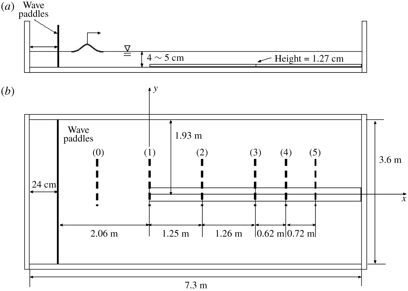
The laboratory experiments are performed in a wave tank that is 7.3 m long, 3.6 m wide and 0.30 m deep, and is elevated 1.2 m above the laboratory floor; the bottom and sidewalls are made of 12.7 mm thick glass plates. A schematic drawing of the apparatus is shown in figure 1; this is the same as the apparatus that is used in Part 1. The wavemaker system is equipped along the 3.6 m long headwall and the piston-type wave paddles are driven by linear motors. The maximum horizontal stroke for the wave paddles is 55 cm, adequate for the generation of long waves in a water depth of  $h_{0}=4.0$–
 $5.0~\text{cm}$: the depths used for the present experiments. The generated waves are repeatable with the maximum error being less than 0.1 % of the depth for solitary waves as reported by Li, Yeh & Kodama (Reference Li, Yeh and Kodama2011). Furthermore, precision of the horizontal bed enables us to create a uniform quiescent water depth throughout the tank, which is critical for the study of long waves. As shown in figure 1, an elongated submerged sill is placed along the centreline of the tank and begins at 2.06 m to the right of the wave paddle. The submerged sill is made of a glass plate that is 5.0 m long, 0.3175 m wide and 0.0127 m thick. The centreline of the sill is located at 1.93 m from the sidewall, which is slightly off from the exact centreline of the tank but should not affect the wave condition examined here.
Schematic drawings of the experimental set-up: (a) elevation view; (b) plan view. The measurement locations are represented as thick dashed lines designated (0), (1), (2), (3), (4) and (5).

The origin of the coordinates is set at the centre of the upstream end of the sill as shown in figure 1;  $x$ points in the direction of wave propagation and
 $y$ points in the lateral direction. The breadth of the submerged sill (0.3175 m) is denoted by
 $D_{0}$ and the thickness (0.0127 m) by
 $b_{0}$. Note that dimensional quantities are denoted with the subscript ‘0’. Unless otherwise stated, all the parameters are normalized with the quiescent water depth
 $h_{0}$ and the time scale
 $\sqrt{h_{0}/g}$, where
 $g$ is the gravitational acceleration.
To generate clean solitary waves, we apply the higher-order solution derived by Grimshaw (Reference Grimshaw1971). In terms of the normalized water-surface elevation  $\unicode[STIX]{x1D702}$, this can be written as
 $$\begin{eqnarray}\unicode[STIX]{x1D702}=a_{i}s^{2}-{\textstyle \frac{3}{4}}a_{i}^{2}(s^{2}-s^{4})+a_{i}^{3}\left({\textstyle \frac{5}{8}}s^{2}-{\textstyle \frac{151}{80}}s^{4}+{\textstyle \frac{101}{80}}s^{6}\right),\end{eqnarray}$$
where  $a_{i}$ is the wave amplitude to be generated normalized by the depth
 $h_{0}$,
 $s=\operatorname{sech}(\unicode[STIX]{x1D705}(x-Ft))$,
 $F=1+\frac{1}{2}a_{i}-\frac{3}{20}a_{i}^{2}+\frac{3}{56}a_{i}^{3}$,
 $\unicode[STIX]{x1D705}=\sqrt{\frac{3}{4}a_{i}}\left(1-\frac{5}{8}a_{i}+\frac{71}{128}a_{i}^{2}\right)$,
 $x$ is the propagation distance and
 $t$ is time. With
 $\unicode[STIX]{x1D702}$ obtained from (2.1), the depth-averaged fluid velocity is computed by
 $\bar{u}=F\unicode[STIX]{x1D702}/(1+\unicode[STIX]{x1D702})$, which allows us to find the wave-paddle displacement,
 $x=\unicode[STIX]{x1D709}(t)$, by integrating
 $\text{d}\unicode[STIX]{x1D709}/\text{d}t=\bar{u}(\unicode[STIX]{x1D709},t)$. As shown in Part 1 and also by Li et al. (Reference Li, Yeh and Kodama2011) and Chen & Yeh (Reference Chen and Yeh2014), this wave generation algorithm together with the precision wave generation system can produce clean solitary waves with negligibly small unwanted trailing noise.
The time evolution of the water-surface elevation  $\unicode[STIX]{x1D702}$ along the submerged sill is measured using the laser-induced fluorescence (LIF) technique. A laser beam is converted to a laser sheet by a cylindrical lens, which is then directed to the desired plumb plane with the use of front-face mirrors. This thin laser sheet illuminates the dyed water from above, then the dissolved fluorescein in the illuminated plane is activated and becomes fluorescent. The water surface along the illuminated ‘line’ is captured with a high-speed video camera (100 fps;
 $1280~\text{H}\times 1024~\text{V}$ pixels): note that for breaking waves discussed in § 5, we used a different camera (125 fps;
 $1024~\text{H}\times 1024~\text{V}$). The water surface is determined as the elevation of maximum gradient in light intensity. Sub-pixel estimation of the water surface is used to remove the stair-step artifact created by integer pixel sampling. To circumvent the difficulty in capturing sufficient vertical resolution for the small vertical scale (i.e. amplitude) relative to the horizontal scale (i.e. wavelength), we repeat the experiments to obtain LIF water-surface profiles on approximately 27 cm segments, and the resulting staggered images make a montage of the five-segment profiles to cover the 120 cm long transect in the lateral direction. The LIF technique implemented here has been proven to yield precise wave measurements successfully in this laboratory environment (for more details, see Li et al. (Reference Li, Yeh and Kodama2011), Chen & Yeh (Reference Chen and Yeh2014) and Chen, Zhang & Yeh (Reference Chen, Zhang and Yeh2014)).
3 Laboratory results
The LIF measurements are made along the  $y$ direction at five
 $x$ locations as depicted in figure 1. Only one side of each wave profile (
 $y\gtrsim 0^{-}$) is measured because the wave pattern should be symmetric about
 $y=0$. Solitary waves with wave amplitude
 $a_{i}=0.1$, 0.2, 0.3 and 0.4 are generated in two different still water levels
 $h_{0}=4.0$ and 5.0 cm. Normalized heights of the sill are
 $b=(b_{0}/h_{0})=0.3175$ when
 $h_{0}=4.0~\text{cm}$ and
 $b=0.254$ when
 $h_{0}=5.0~\text{cm}$. From hereon in, we normalize the water-surface displacement
 $\unicode[STIX]{x1D702}$ and the wave amplification
 $\unicode[STIX]{x1D6FC}$ with the initial amplitude
 $a_{i}$ generated by the wavemaker system. For the cases of
 $a_{i}\gtrsim 0.4$ in
 $h_{0}=5.0~\text{cm}$ (
 $b=0.254$) and
 $a_{i}\gtrsim 0.3$ in
 $h_{0}=4.0~\text{cm}$ (
 $b=0.3175$), the generated wave breaks on the submerged sill. To study the transformation of the solitary wave travelling along the sill, we focus on examining the following two cases that involve no wave breaking. Namely, Case A:
 $a_{i}=0.3$ with
 $D=6.34$ and
 $b=0.254$ for
 $h_{0}=5.0~\text{cm}$; and Case B:
 $a_{i}=0.2$ with
 $D=7.925$ and
 $b=0.3175$ for
 $h_{0}=4.0~\text{cm}$. Note that
 $D$ is the breadth of the submerged sill and
 $b$ is the thickness. Detailed wave-breaking processes and characteristics for the case of
 $a_{i}=0.4$ in
 $h_{0}=5.0~\text{cm}$ (
 $b=0.254$) are captured with the LIF technique and presented separately in § 5.
3.1 Water-surface profiles
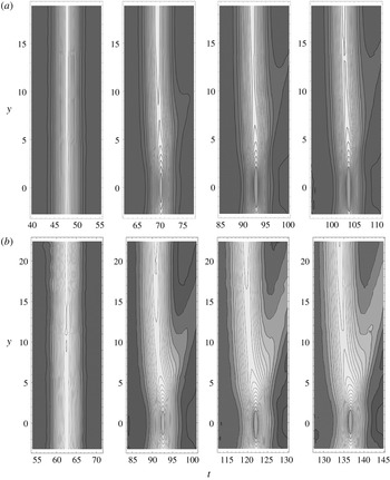
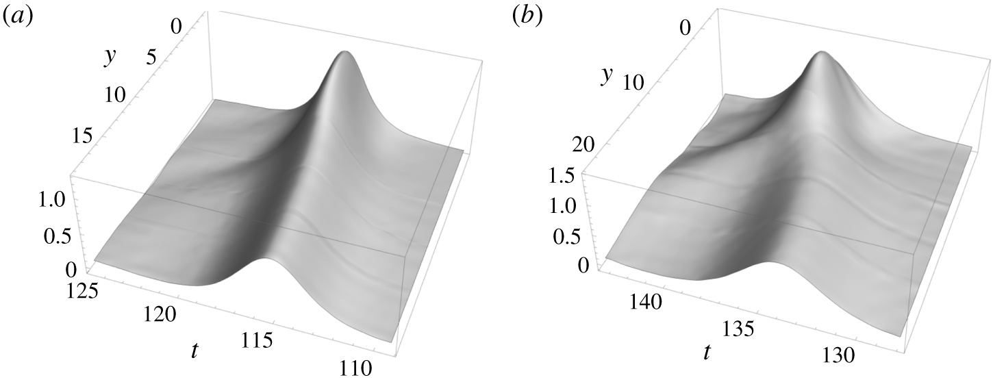
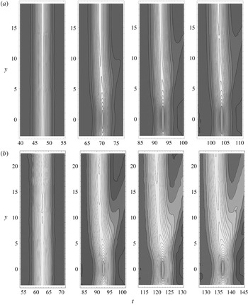
Figure 2 shows the water-surface contours based on the data obtained with the LIF technique at  $x=0$, 25.0, 50.2 and 62.6 (corresponding to the positions (1), (2), (3) and (4) in figure 1) for Case A, and at
 $x=0$, 31.25, 62.75 and 78.25 for Case B. (The contour data at position (5) are not shown because the complete water surface was not successfully captured for Case B: no additional information could be gained from the data at position (5).) The amplification profile
 $\unicode[STIX]{x1D6FC}$ (maximum water-surface elevation normalized by initial wave amplitude) along the
 $y$ transect, and the temporal variation of the water-surface elevation
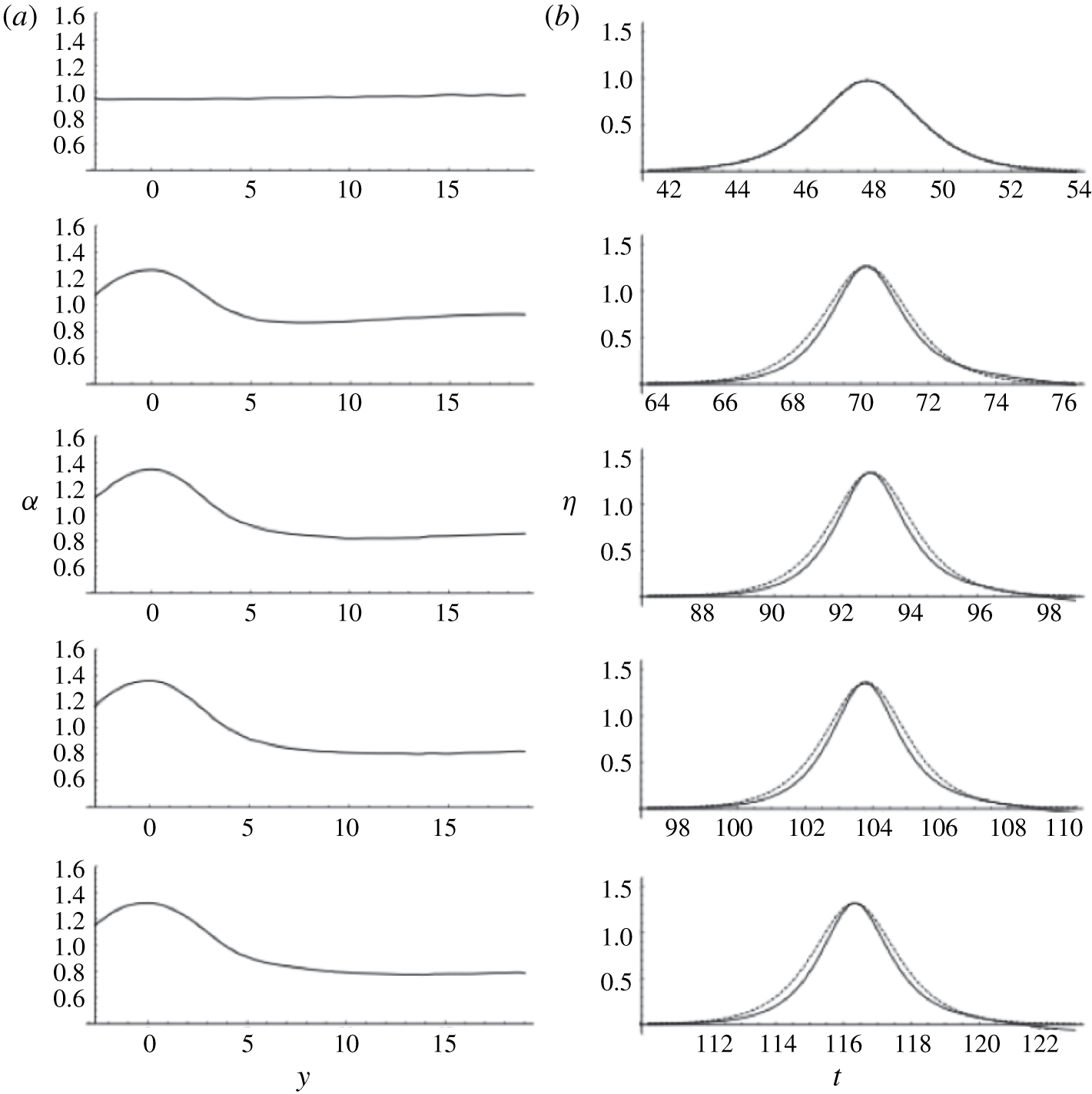
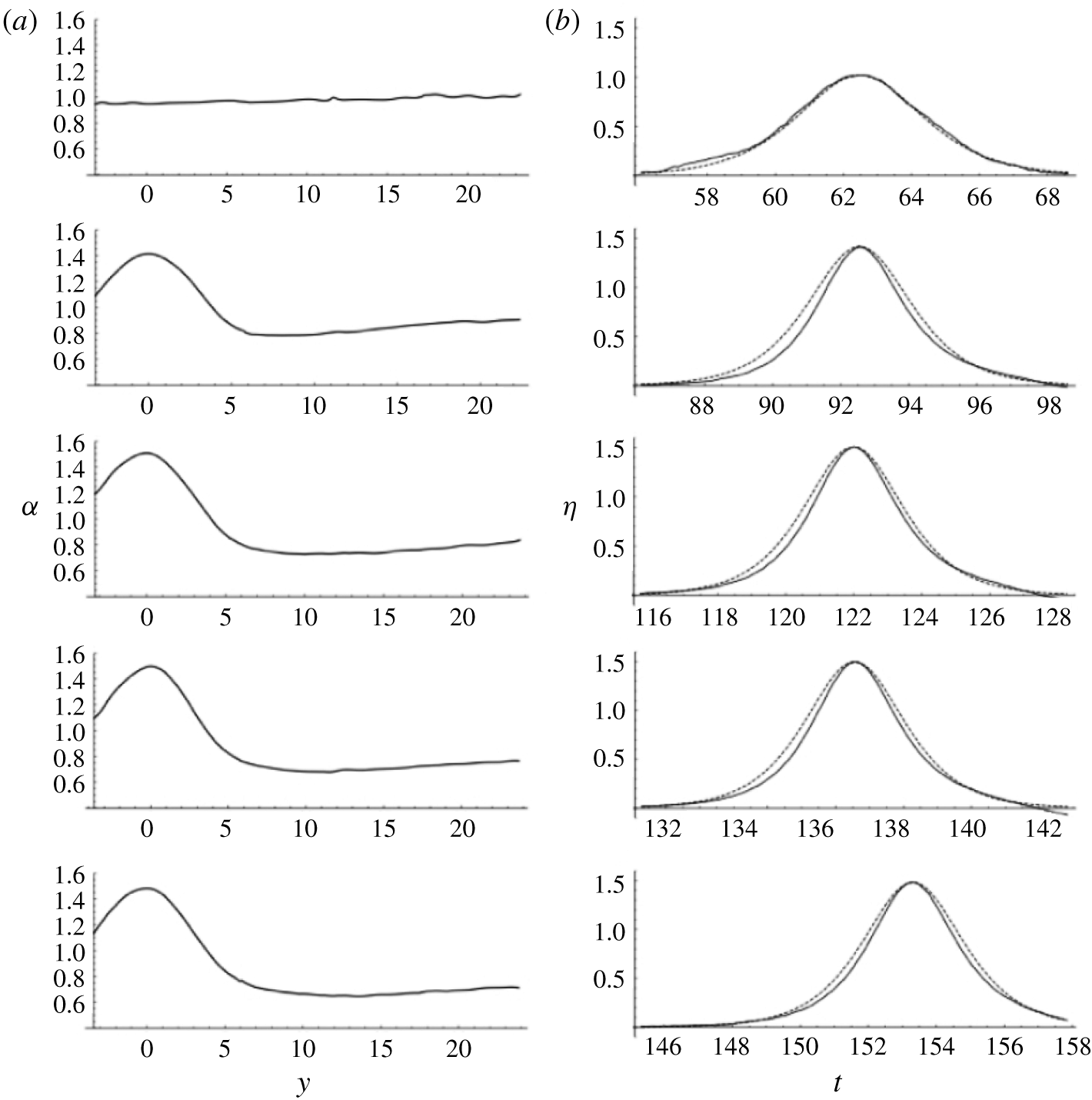
 $\unicode[STIX]{x1D702}$ at the centreline of the sill are shown in figures 3 and 4 for Cases A and B, respectively. Note that in figures 2–4,
 $y=0$ is at the location of the centre of the sill. The edge of the sill is at
 $y=3.17$ for Case A and
 $y=3.96$ for Case B. (Note that the temporal profile at
 $y=0$ and
 $x=96.25$ for Case B is shown with a slight time shift, because the profile behind the wave
 $t\geqslant 158$ could not be captured with the LIF operation as mentioned earlier.)
Contour plots of the water-surface elevation during the evolution of the solitary wave. (a) Case A with  $a_{i}=0.3$ in
 $h_{0}=5~\text{cm}$ disturbed by the sill with
 $D=6.34$ and
 $b=0.254$. The plots from left to right are at
 $x=0$, 25.0, 50.2 and 62.6. (b) Case B with
 $a_{i}=0.2$ in
 $h_{0}=4~\text{cm}$ disturbed by the sill with
 $D=7.925$ and
 $b=0.3175$. The plots from left to right are at
 $x=0$, 31.25, 62.75 and 78.25. The origin
 $y=0$ is taken at the centre of the sill, and the edge of the sill is located at
 $y=3.17$ for Case A and
 $y=3.96$ for Case B.
Water-surface profiles for Case A with  $a_{i}=0.3$ in
 $h_{0}=5~\text{cm}$ disturbed by the sill with
 $D=6.34$ and
 $b=0.254$. From top to bottom: at
 $x=0$, 25.0, 50.2, 62.6 and 77.0. (a) Amplification
 $\unicode[STIX]{x1D6FC}$ in
 $y$ (maximum
 $\unicode[STIX]{x1D702}$). (b) Temporal variation of the water-surface elevation
 $\unicode[STIX]{x1D702}$ at the centre of the sill. The origin
 $y=0$ is taken at the centre of the sill, and the edge of the sill is located at
 $y=3.17$. The time origin is consistent for all the panels.

Water-surface profiles for Case B with  $a_{i}=0.2$ in
 $h_{0}=4~\text{cm}$ disturbed by the sill with
 $D=$ 7.925 and
 $b=0.3175$. From top to bottom: at
 $x=31.25$, 62.75, 78.25 and 96.25. (a) Amplification
 $\unicode[STIX]{x1D6FC}$ in
 $y$ (the maximum
 $\unicode[STIX]{x1D702}$). (b) Temporal variation of the water-surface elevation
 $\unicode[STIX]{x1D702}$ at the centre of the sill. The origin
 $y=0$ is taken at the centre of the sill, and the edge of the sill is located at
 $y=3.96$. The time origin is consistent for all the panels.

The following observations are made from figures 2–4. Wave amplification occurs over the sill, and the phase of the wave on the sill lags behind the ambient wave. Detailed discussions on the wave amplification and the phase difference are presented in §§ 3.2 and 3.3. The following are some subtle features. First, the temporal wave profiles shown in figures 3(b) and 4(b) indicate that the waveform on the sill becomes narrower than that of a solitary wave. Notice that the solitary wave observed at  $x=0$ almost perfectly matches the prediction (2.1). The slightly distorted wave profile on the leading front of Case B shown in figure 4(b) at
 $x=0$ is possibly caused by the wave reflection at the step of the front face of the sill.
Careful examination of figures 3(a) and 4(a) reveals that the wave amplitude is smallest away from the edge of the obstacle: the amplitude is smaller than that of the ambient waves, i.e.  $\unicode[STIX]{x1D6FC}<1$. The smallest amplitude is at
 $y=(7.74,10.17,13.50,13.84)$ at
 $x$ locations of (25.0, 50.2, 62.6, 77.0), respectively, for Case A (figure 3a). For Case B (figure 4a), we find the minimum wave amplitude at
 $y=(8.06,10.04,11.49,13.56)$ at
 $x$ locations of (31.25, 62.75, 78.25, 96.25), respectively. Evidently, the farther the propagation, the farther apart the location of minimum amplitude from the edge of the sill. We also note that at
 $x=0$ (the front edge of the sill), the wave amplitude at the sill (
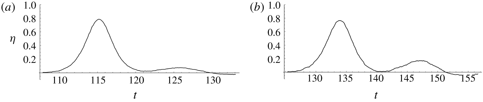
 $y=0$) is, though very subtle, smaller than the ambient value for both Cases A and B. The expanding pattern of the location of the amplitude depression resembles the formation of a ‘wake’ created at the collision of the solitary wave with the leading edge of the sill. Also observed in figures 2(a) and 2(b) is the formation of a radiating wave off the side edge of the sill, which can be clearly shown in figure 5. In addition, figures 6(a) and 6(b) show the temporal wave profiles of Cases A and B, respectively, taken at a location far away from the sill. Each figure exhibits the leading ambient solitary wave propagating parallel to the sill, followed by the radiating wave from the edge of the sill. The amplitude ratio of the radiating wave to the ambient solitary wave is 0.096 for Case A and 0.225 for Case B. Clearly, substantial wave energy radiates from the sill, especially for Case B. As will be discussed in § 3.2, the continually radiating waves play a critical role in the attenuation of the ambient solitary wave.
Three-dimensional perspective view of the water-surface profile. (a) Case A:  $a_{i}=0.3$ in
 $h_{0}=5~\text{cm}$ at
 $x=77.0$. (b) Case B:
 $a_{i}=0.2$ in
 $h_{0}=4~\text{cm}$ at
 $x=78.25$.

Temporal water-surface profile at the location away from the sill: the leading wave is the ambient solitary wave followed by the wave radiating from the edge of the sill. (a) Case A at  $y=18.4$ and
 $x=77.0$. (b) Case B at
 $y=23.7$ and
 $x=78.25$.

3.2 Amplitude evolution
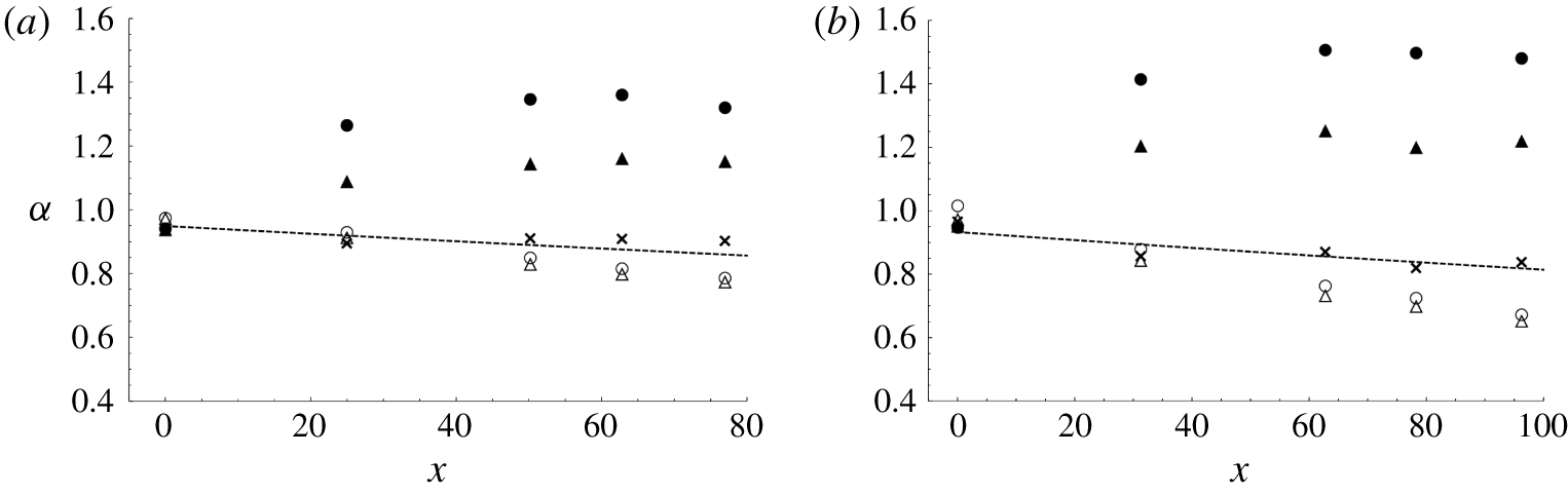
Figure 7 shows the amplitude evolution of a solitary wave along various transverse locations for Cases A and B. The amplitude at the centre of the sill quickly increases, and then reaches its equilibrium amplification followed by a slight decay, while the amplitude of the wave at a distance away from the sill decays continually. The decay rate of the wave at  $y>15$ is faster than that of the unobstructed ambient wave without placing the sill in the tank. The unobstructed decay rate measured in this laboratory apparatus is reported in Part 1, and the measurements are in good agreement with the theoretical predictions based on the laminar boundary layer given by Keulegan (Reference Keulegan1948).
Amplitude variations along the wave propagation at various lateral locations:  $y=0$, ●;
 $y=2.5$, ▴;
 $y=5.0,\times$;
 $y=15$, ▵;
 $y=17.5$, ○. (a) Case A (
 $a_{i}=$ 0.3,
 $b=$ 0.254). (b) Case B (
 $a_{i}=0.2$,
 $b=0.3175$). Amplitude decay of the free solitary wave predicted by Keulegan (Reference Keulegan1948) is shown with a dashed line.

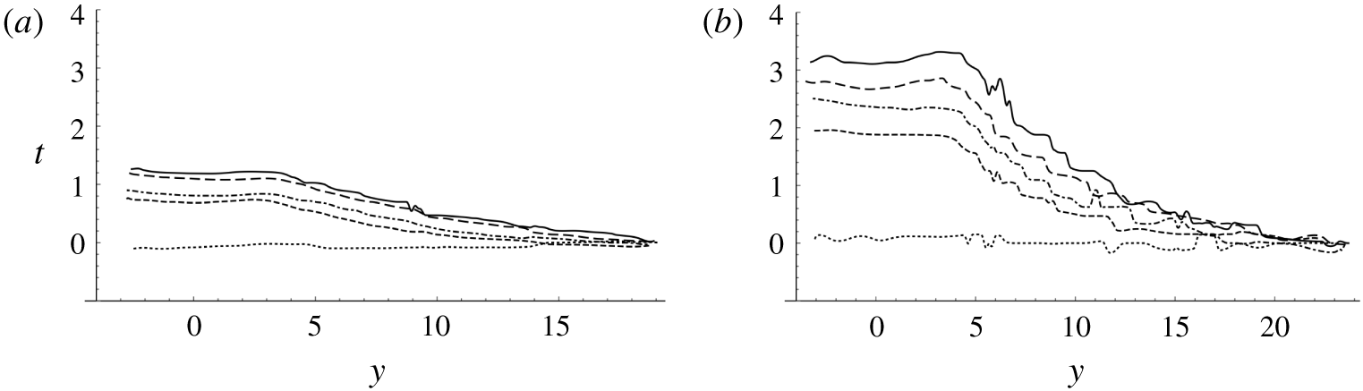
Trace of the maximum amplification along the lateral ( $y$) direction, which represents a phase shift in time. (a) Case A (
 $a_{i}=0.3$,
 $b=0.254$):
 $y=0$ is at the centre of the sill and
 $y=3.17$ at the edge of the sill. Solid line,
 $x=77.0$; long dashed line,
 $x=62.6$; dash-dot line,
 $x=50.2$; short dashed line,
 $x=25.0$; dotted line,
 $x=0$. (b) Case B (
 $a_{i}=0.2$,
 $b=0.3175$):
 $y=0$ is at the centre of the sill and
 $y=3.96$ at the edge of the sill. Solid line,
 $x=96.25$; long dashed line,
 $x=78.25$; dash-dot line,
 $x=62.75$; short dashed line,
 $x=31.25$; dotted line,
 $x=0$.

According to Keulegan (Reference Keulegan1948), the amplitude of a solitary wave decays as
 $$\begin{eqnarray}a^{-1/4}-a_{i}^{-1/4}=Kx,\end{eqnarray}$$
where
 $$\begin{eqnarray}K=\frac{1}{12}\sqrt{\frac{\unicode[STIX]{x1D708}}{g^{1/2}h_{0}^{3/2}}},\end{eqnarray}$$
for a very wide channel, and  $\unicode[STIX]{x1D708}$ is the kinematic viscosity of water. In (3.1),
 $a$ is the wave amplitude after travelling a distance
 $x$ and
 $a_{i}$ is the initial wave amplitude.
3.3 Phase lag
Figure 8 shows the loci of maximum water-surface elevation (i.e. wave crest) in the  $y{-}t$ plane, representing the phase difference in the
 $y$ direction. Note that we set the time origin at the arrival time of wave crest at the farthest
 $y$ location of the measurements. The results show that for both Cases A and B, the phase along the sill lags behind the ambient wave phase, and the phase lag does not appear to reach its equilibrium state. In other words, the phase lag continues even at the farthest measurement location in the tank. The phase difference shown in figure 8 is more severe for Case B (
 $b=0.3175$), simply because the difference in phase speed between the ambient location and over the sill is greater than for Case A (
 $b=0.254$). The phase lag of the wave over the sill increases as the wave continues to propagate and it appears that this lag growth continues with no signs of slowing down.
4 Numerical extension
Motivated by the foregoing laboratory findings, numerical simulations for Case B ( $a_{i}=0.2$,
 $b=0.3175$) are performed for three different sill configurations to gain further insight into the interaction between the solitary wave and the sill. Based on the laboratory results, Case B is chosen for the numerical experiments because it prominently features evolution processes. A higher-order pseudo-spectral method developed by Dommermuth & Yue (Reference Dommermuth and Yue1987) is implemented to numerically solve the full water-wave Euler equations. This numerical scheme has been demonstrated to yield very accurate results for transformations of solitary waves in various situations (see e.g. Tanaka Reference Tanaka1993; Jia Reference Jia2014; Knowles & Yeh Reference Knowles and Yeh2019). The pseudo-spectral method is known to conserve mass and to induce little numerical energy dissipation. The method takes advantage of the fast Fourier transform, and is robust for the long-time evolution of water-wave problems (Craig & Sulem Reference Craig and Sulem1993; Guyenne & Nicholls Reference Guyenne and Nicholls2005). Therefore, the pseudo-spectral method allows us to significantly expand our computational domain and to study the asymptotic nature of the solitary wave propagating along the sill, a much longer propagation distance than the observations made in the laboratory wave tank.
A brief description of this numerical algorithm is presented in appendix A. The initial conditions as well as the basis functions used in the numerical experiments must be smooth and analytic, so spectral accuracy can be expected. The Euler formulation also implicitly neglects the effects of viscosity which allows us to extract the effects of wave attenuation from radiation alone without viscous dissipation.
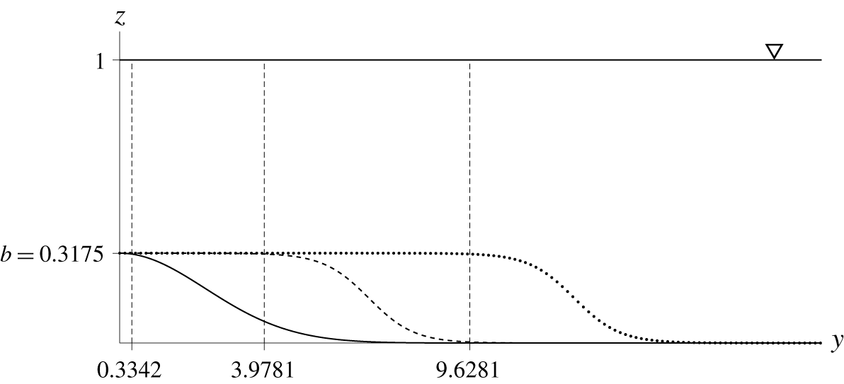
It must be recognized, however, that because the Fourier transform is used in the algorithm, the pseudo-spectral method cannot incorporate exactly the rectangular-shaped submerged sill because of its discontinuity in depth: recall the instability associated with the Gibbs effect that is inherent to the Fourier transform. Furthermore, the formulation assumes that the gradient of the bathymetry is small and defined everywhere, which prohibits us from having a discontinuity in the sill. The depth discontinuity in the lateral direction is especially sensitive in the numerical algorithm. Therefore, we use sill models with adequately smooth shapes in the numerical experiments, which are shown in figure 9, referred to as ‘narrow’, ‘moderate’ and ‘wide’, while the height  $b$ of each sill is kept the same. The ‘moderate’ sill configuration used in the numerical simulation is similar to but not exactly the same as the one used in the laboratory experiment; hence the results presented here should only be compared qualitatively with the laboratory results. There is no clearly defined width for the sills in the numerical experiments. Here we define the ‘edge’ of the sill to be the location at
 $y=y_{e}$ where the bathymetry attains a value of 99 % of the step height
 $b$.
A sketch of the  $y$ cross-section of the three sills used for the numerical simulations. The ‘narrow’ sill is represented by a solid line, the ‘moderate’ sill by a dashed line and the ‘wide’ sill by a dotted line. Because of symmetry, only half of the domain is simulated. The moderate and wide sills are modelled by the hyperbolic tangent curve. The narrow sill is modelled by the Gaussian shape to avoid discontinuity in slope at
 $y=0$. The vertical dashed lines represent the location of the ‘edge’ of the sills (
 $y_{e}=0.3342$, 3.9781 and 9.6281), and the edge is defined by the location at 99 % of the step height
 $b$.

4.1 Numerical results
For the numerical simulations, a solitary wave specified by (2.1) with an incident wave amplitude of  $a_{i}=0.2$ is introduced such that the crest of the wave initiates at
 $x=-52.9$. The spatial resolutions in the
 $x$ and
 $y$ directions are
 $\text{d}x=0.365$ and
 $\text{d}y=0.3775$, respectively, and a time step of
 $\text{d}t=0.078$ is used; the resulting Courant–Friedrichs–Lewy number is less than 0.21. The numerical simulations are performed such that the wave propagates for a very long distance until the leading crest reaches the location
 $x=2300$ (or 92 m); recall that the maximum propagation length available in the present laboratory wave tank is 125 (or 5 m). The breadth of the computational domain is kept the same as in the laboratory experiments, i.e. the Neumann boundary conditions are imposed at
 $y=0$ and
 $y=48.25$ (1.93 m). This lateral confinement of the domain means that the wave energy is finite: no energy is supplied or depleted at the boundary.
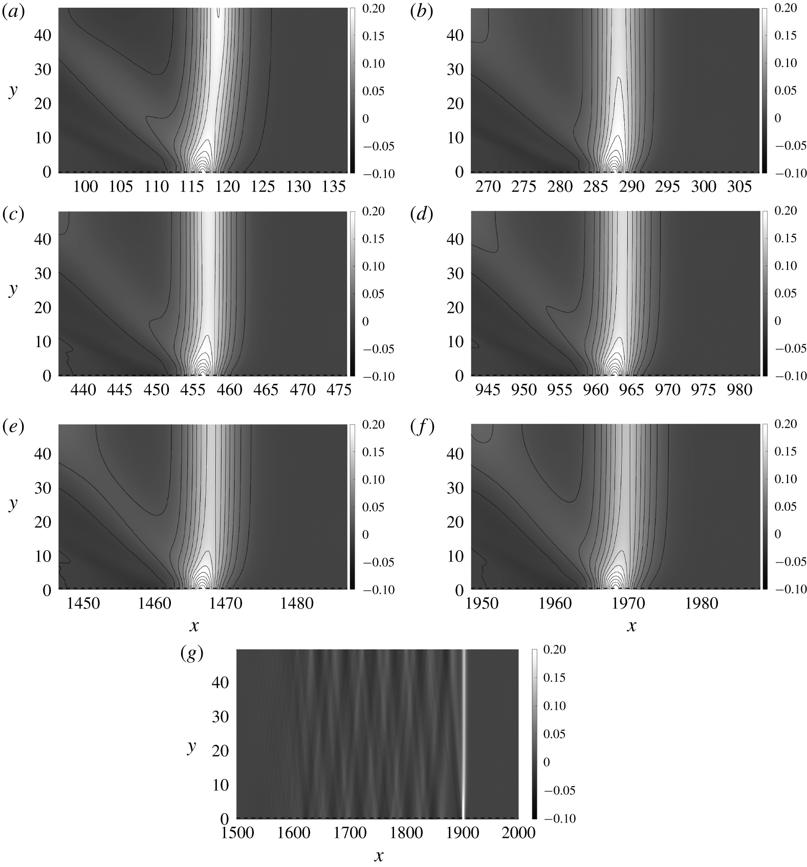
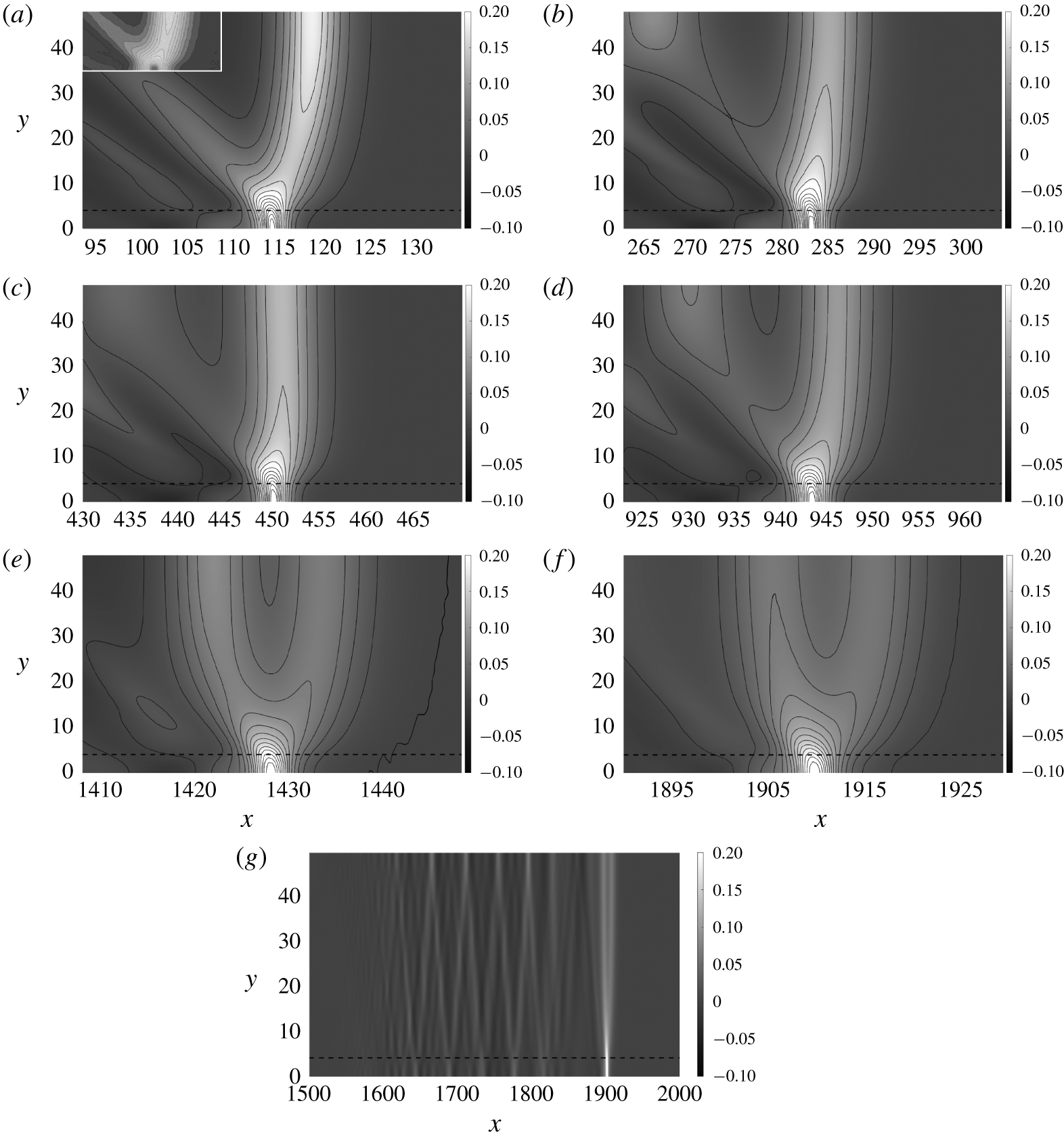
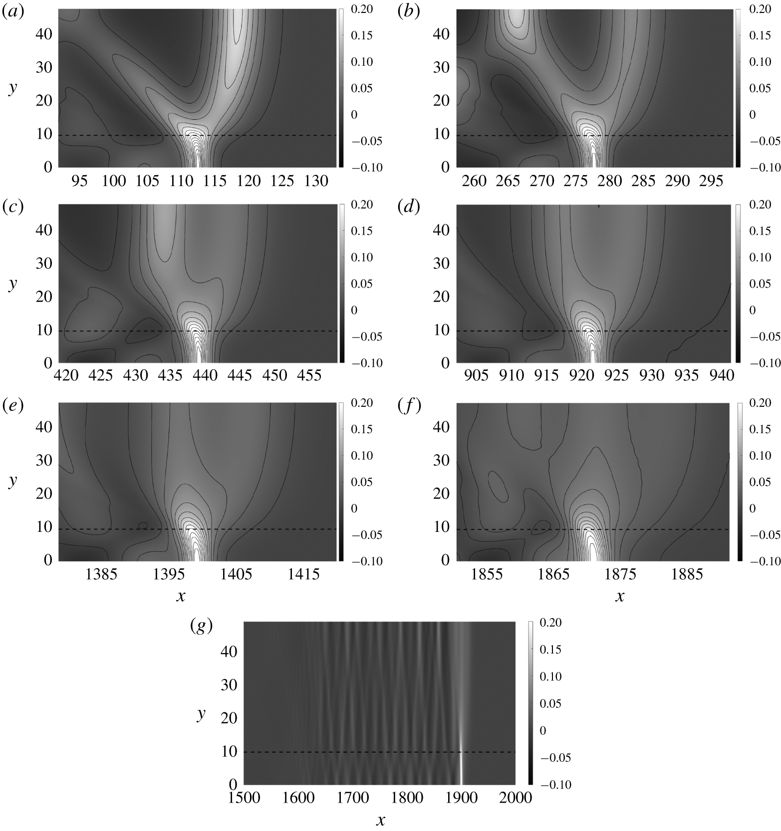
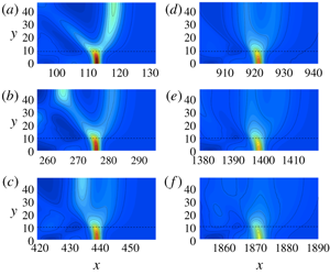
Figures 10, 11 and 12 show contour plots of the water surface at selected times for the ‘narrow’, ‘moderate’ and ‘wide’ sills, respectively. Note that the breadth of the moderate sill ( $y_{e}=3.9781$; see figure 9) is close to the breadth (
 $y_{e}=7.925/2=3.9625$) of the rectangular-shaped sill used in the laboratory experiments; hence, we first discuss the results shown in figure 11. The wave pattern observed at
 $t=156.6$ in figure 11(a) for the moderate sill is very similar to what is observed in the laboratory at around the same time: see the inset of figure 11(a) presenting the contour plot based on the laboratory data shown in figure 5(b). Like the laboratory observation, figure 11(a) shows that the radiating waves are generated in the vicinity of the edge of the sill as well as from the centre of the sill. The wave amplitude decays over time despite the lack of viscosity in the numerical simulation. The wave pattern gradually changes as the wave propagates. The initial wave pattern, that is the ambient offshore leading wave, is no longer sustained after a long propagation time (
 $t\gtrsim 1400$; see figure 11e,f). It appears that the initially generated solitary wave is eventually annihilated because of the wave radiation caused by the presence of the sill.
Contour plots of the water surface for Case B with a ‘narrow’ sill, travelling in an extended domain. The dashed line represents the ‘edge’ of the sill ( $y_{e}=0.3342$). Snapshots of the leading wave are presented at times: (a)
 $t=156.6$, (b) 313.2, (c) 469.8, (d) 939.6, (e) 1409.4 and (f) 1879.3; (g) a wide-range plot of the water surface at
 $t=1816.6$.

Contour plots of the water surface for Case B with a ‘moderate’ sill, travelling in an extended domain. The dashed line represents the ‘edge’ of the sill ( $y_{e}=3.9781$). Snapshots of the leading wave are presented at times: (a)
 $t=156.6$, (b) 313.2, (c) 469.8, (d) 939.6, (e) 1409.4 and (f) 1879.3; (g) a wide-range plot of the water surface at
 $t=$ 1871.4. The inset in (a) shows the laboratory LIF data corresponding to figure 5(b).

Contour plots of the water surface for Case B with a ‘wide’ sill, travelling in an extended domain. The dashed line represents the ‘edge’ of the sill ( $y_{e}=9.6281$). Snapshots of the leading wave are presented at times: (a)
 $t=156.6$, (b) 313.2, (c) 469.8, (d) 939.6, (e) 1409.4 and (f) 1879.3; (g) a wide-range plot of the water surface at
 $t=1909.0$.

On the other hand, the waveform in the case of the narrow sill maintains its pattern with the gradual reduction in the leading-wave amplitude, as shown in figure 10. It appears that energy radiation is not large enough to prevent the leading wave from maintaining its form for a long time. On the other hand, the moderate and wide cases (see figures 11 and 12) clearly show a change in wave pattern that behaves differently in time and space. For the case of the wide sill (figure 12), the substantial energy radiation quickly changes the wave pattern of the leading wave, sending the energy back to the trailing waves. Consequently, the leading solitary wave is annihilated quickly for the case of the wide sill.
Figures 10(g), 11(g) and 12(g) show the entire wave pattern at  $t=1816.6$,
 $t=1871.4$ and
 $t=1909.0$ for the narrow-, moderate- and wide-sill cases, respectively. Note that these times correspond to when the crest of the waveform has reached the location of
 $x\approx 1900$. Figure 10(g) (narrow sill) shows the distinct leading-wave formation together with the regularly forming trailing waves, created by the radiation, that are bouncing between the lateral boundaries. In the case of the moderate sill (figure 11g), the leading ambient solitary wave appears to be of the same magnitude as the first trailing wave, owing to the deterioration of wave energy by radiation. As for the wide sill (figure 12g), the ambient leading wave is no longer identified clearly, although the wave on the sill still maintains itself distinctly. For all three cases, the wave trains created by radiation are trailing the leading wave.
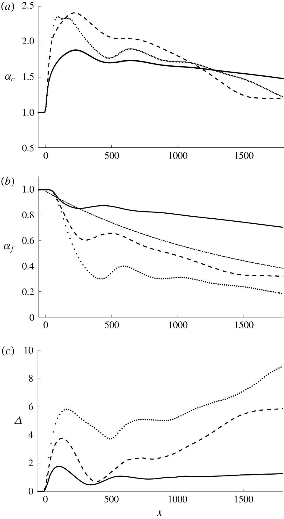
Figure 13(a) shows the wave-amplitude variations at the centre of the sill ( $y=0$) for the three different sill configurations. There is an initial amplification in wave amplitude for each case. The smallest amplification occurs for the narrow-sill case and the greatest amplification appears for the moderate-sill case. In the wide-sill case, we see that the amplitude reaches a maximum earlier than for the other cases. This can be explained by the following. The initial amplification for the wide-sill case can be due mainly to shoaling associated with the relatively broad front face of the sill, whereas the front face of the narrow- and moderate-sill cases is too narrow for shoaling to be effective. Instead, the wave amplification must be caused by focusing the refracted waves from the sides of the sill after the wave passes the front face of the sill. The initial amplification for the moderate-sill case can be explained in terms of the contributions of both shoaling and focusing effects, resulting in the highest amplification among the three cases simulated.
Variations of amplification (a)  $\unicode[STIX]{x1D6FC}_{c}$ at the centre of sill (
 $y=0$) and (b)
 $\unicode[STIX]{x1D6FC}_{f}$ at far offshore location (
 $y=y_{f}$). (c) The spatial phase difference
 $\unicode[STIX]{x1D6E5}$ between the leading wave at the centre of the sill and the offshore location
 $y=y_{f}$. Narrow-sill case, solid line; moderate-sill case, dashed line; wide-sill case, dotted line. The dash-dot line represents the amplitude decay by viscous effect predicted by Keulegan (Reference Keulegan1948).

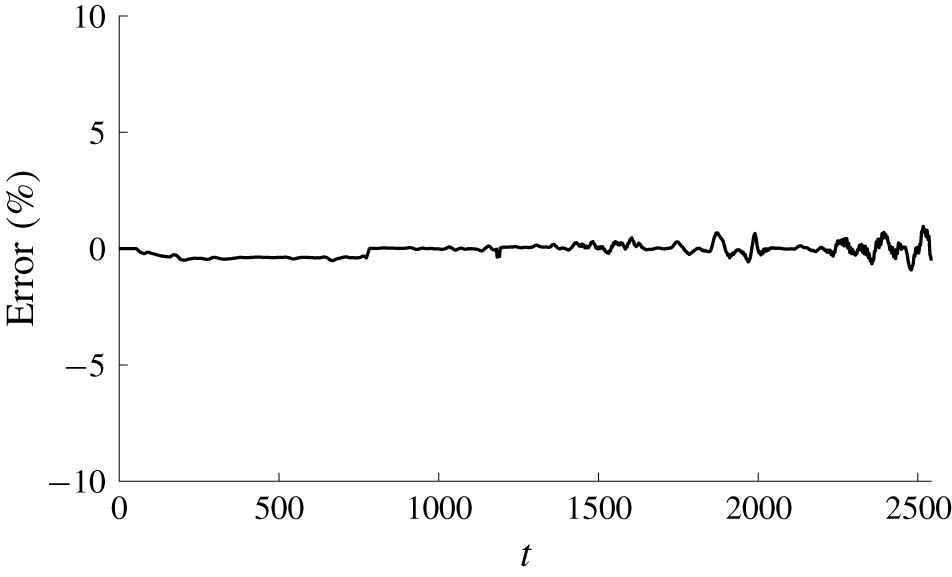
Relative error of total energy over the entire domain for Case B with a ‘moderate’ sill width, demonstrating that energy is conserved for the numerical simulation.

The amplitude evolution of the case with the narrow sill along the centre of the sill ( $y=0$) in figure 13(a) shows that the initial wave amplification (
 ${\approx}1.84$) is smaller than that for the broader sills (
 ${\approx}2.41$ and 2.36 for the moderate and wide sills, respectively), but remains nearly uniform afterwards with only slight attenuation. Eventually the amplitude on the sill for the narrow-sill case exceeds those of the moderate- and wide-sill cases (
 $x\gtrsim 1300$).
In figure 13(b) we plot the amplitude at an offshore location for the three different sill configurations. The offshore location  $y_{f}$ for each case is determined conveniently by
 $y_{f}=y_{e}+30$, where the value of 30 is chosen because this value provides a location which is far enough out from the sill to capture the ambient behaviour of the incident wave. Note that the bathymetry at this location is practically flat, and therefore has little effect on the waveform. We also plot the prediction for amplitude decay from viscous effects given by Keulegan (Reference Keulegan1948) presented in (3.1) with (3.2). Note that there is no viscous energy dissipation in the numerical simulations based on the Euler formulation model. For the narrow-sill case, the wave attenuation caused by the radiation is significantly slower than the viscous decay. For the moderate-sill case, the attenuation rate by radiation is comparable with the viscous decay rate. And the initial radiation effect is much greater than the viscous attenuation for the wide-sill case, but soon after (
 $x\gtrsim 600$) the decay rate becomes comparable with the viscous decay just like the case with the moderate sill.
Figure 13(c) shows the phase difference (the difference in space of the wave crest) between the centre of the sill and the ambient location at  $y_{f}$. The difference in magnitude and behaviour among the cases with three different sills is evident. For the narrow sill, the phase lag of the wave on the sill reaches its peak value at
 $x=106$, prior to the peak in wave amplification (
 $x=231$). The phase difference subsides while the amplification on the sill increases, hence the increase in propagation speed. The wave system then reaches a quasi-steady state where a gradual reduction in wave amplitude is still observed. It is emphasized that the phase difference in space throughout the evolution remains small,
 $\unicode[STIX]{x1D6E5}\approx 1$, after the initial maximum value of
 $\unicode[STIX]{x1D6E5}=1.78$. There is a similar initial evolution pattern in phase difference for the moderate- and wide-sill cases which can be seen in figure 13(c), but the phase on the sill continually lags behind the ambient wave at a faster rate; hence, the phase difference at later times eventually exceeds the initial difference. Unlike for the narrow sill, the evolution process for the moderate- and wide-sill cases never shows any sign of a quasi-equilibrium state (although the phase separation rate gradually slows down for the moderate case after
 $t\approx 1500$). The wave on the sill continually lags behind the ambient wave. The magnitude of the phase difference throughout the evolution is much greater than that for the case of the narrow sill. Moreover, the phase difference for the wide-sill case is larger than that for the moderate-sill case.
It is emphasized that the numerical model is based on the Euler formulation; hence no energy dissipation is included in the model. Figure 14 shows the total energy in the entire computational domain, which clearly demonstrates little energy dissipation (a maximum relative error of 0.95 %). Increasing fluctuation of the error shown in figure 14 presumably results from the numerical manipulation of the patching operation which is used to achieve a very long numerical simulation; for the patching operation, see appendix A. Furthermore, it is progressively more difficult to accurately calculate small amounts of energy that are distributed in a broad domain.
5 Breaking wave
Here we present our laboratory study of wave breaking on the longitudinally oriented sill for the case with  $a_{i}=0.4$ in
 $h_{0}=5.0~\text{cm}$ (
 $b=0.254$). We have performed another experiment for wave breaking for the case with
 $a_{i}=0.3$ in
 $h_{0}=4.0~\text{cm}$ (
 $b=0.3175$). The results are qualitatively consistent with the results presented in this section; hence they are not presented for the sake of brevity. Because the wave-breaking phenomenon on the sill primarily takes place in the vicinity of the sill, the parameters in this section are normalized with the local quiescent water depth on the sill, that is
 $h_{0}$ (on the sill)
 $=3.73~\text{cm}$, instead of 5.0 cm. It is noted that, owing to the relatively small-scale laboratory experiment, wave breaking created here did not cause the water surface to overturn; hence no air bubbles were entrained in the water. This type of breaking is characterized by the formation of parasitic capillary waves (see e.g. Duncan Reference Duncan2001), creating vortical-flow rollers near the surface.
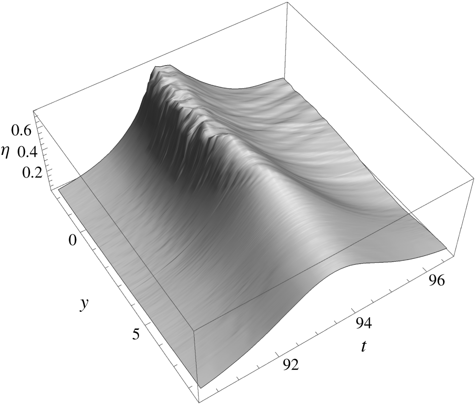
Compiling three LIF segments in the  $y$ direction (the lateral direction) at
 $x=53.6$ yields a montage of water-surface maps in the
 $y{-}t$ plane in the range
 $-2.3<y<19.2$. The resulting spatio-temporal water-surface profile extracted for
 $-2.3<y<8.45$ is shown in figure 15. Note that the centreline of the sill is at
 $y=0$, and the outer edge of the sill is located at
 $y=4.26$. Because of the configuration of the laboratory set-up, the wave pattern should be symmetric about
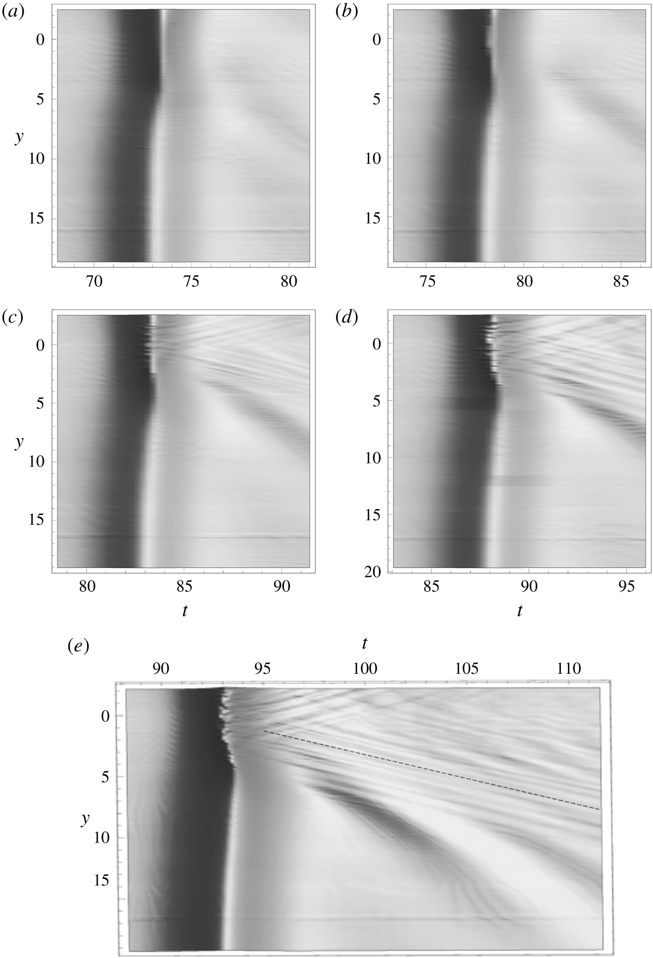
 $y=0$; hence we take the measurements to cover one side of the wave pattern. For the breaking-wave case, LIF data are captured at a rate of 125 frames per second. Details of the breaking wave are not exactly reproducible even in our laboratory apparatus, but gross features in the montage appear to be continuous and the interface of the montage process cannot be detected. The irregular water-surface features that represent the breaking crest can be seen in figure 15, spanning over the entire sill width (
 $y\leqslant 4.26$). There appear to be many streak-like patterns fanning out behind the breaking-wave crest. (Those features are explicitly seen in figure 17, which will be discussed later.) The front face of the breaking wave also exhibits an irregular streak-like pattern. Our LIF technique cannot capture the detailed features of the very steep front of parasitic capillary waves because of blockage of the laser light by the overhanging water surface; the blockage of the laser sheet causes a jump in the water-surface image.
The temporal variation of the water-surface profile in the  $y$ direction (perpendicular to the wave propagation, also to the sill) at
 $x=53.6$. Note that the centreline of the sill is at
 $y=0$, and the edge of the sill is located at
 $y=4.26$.

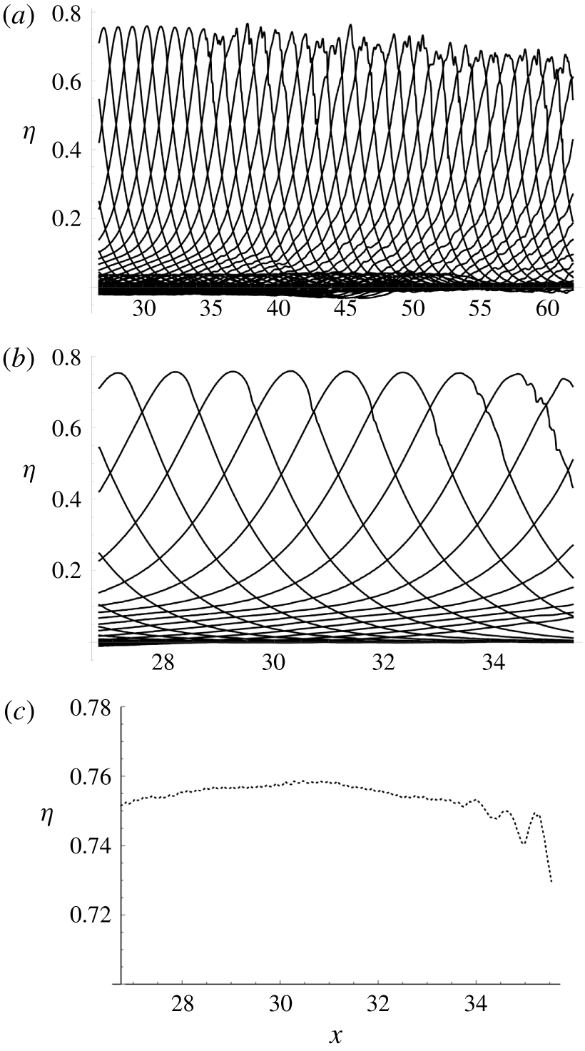
Temporal variation of breaking-wave profile along the centreline of the sill for the initial solitary wave with  $a_{i}=0.4$,
 $h_{0}=5~\text{cm}$. (a) The entire range of the measurement. (b) Detailed profiles for the onset of breaking. (c) Amplitude variation during the onset of breaking.

Spatio-temporal water-surface patterns of the laboratory data obtained with the LIF technique for the initial solitary wave with  $a_{i}=$ 0.4,
 $h_{0}=5~\text{cm}$. The centreline of the sill is at
 $y=0$; the edge of the sill is located at
 $y=4.26$;
 $x=0$ is set at the upstream edge of the sill: (a)
 $x=26.8$, (b) 33.5, (c) 40.3, (d) 46.9 and (e) 53.6. Onset of the breaking is observed at (b)
 $x=33.5$. The dashed line shown in (e) represents the wave speed of
 $23~\text{cm}~\text{s}^{-1}$ for the gravity–capillary waves. Note that the uniform narrow streak appearing around
 $y=17$ is a slight laser sheet disturbance caused by the reflection of the light from the sealant at the bottom of the tank.

Figure 16 shows the temporal variation of the wave profile along the centreline of the sill, exhibiting the breaking process. The onset of breaking is seen near  $x=34$ as shown in figure 16(b), and the variation of wave amplitude during the process is presented in figure 16(c). Gradual but continual growth in wave amplitude can be seen until
 $x=31$, prior to the onset of breaking. It should be noted that the exact timing and location of the incipience of ‘breaking’ are unclear in observation, and ambiguous in terms of the definition of wave breaking. The maximum wave amplitude reaches
 $a=0.759$ prior to the breaking. This wave amplitude is lower than the maximum solitary-wave amplitude of 0.827 given by Longuet-Higgins & Fenton (Reference Longuet-Higgins and Fenton1974). On the other hand, in their laboratory study of the Mach reflection of solitary waves, Li et al. (Reference Li, Yeh and Kodama2011) reported that the maximum amplitude at the reflective vertical wall prior to wave breaking was found to be 0.910, which is greater than the 0.827 of the solitary wave. Note that the wave breaking associated with the Mach reflection is equivalent to the situation of converging two solitary waves with an oblique incidence, which is similar to the present case of a locally converging wave on the sill. But the maximum wave amplification on the sill found in the present study is much smaller than that occurring in a horizontal bed, and even smaller than that of a one-dimensional solitary wave case predicted by Longuet-Higgins & Fenton (Reference Longuet-Higgins and Fenton1974). Incidentally, our additional laboratory experiment on wave breaking with
 $a_{i}=0.3$ in the ambient water depth
 $h_{0}=4.0~\text{cm}$ resulted in a maximum amplitude of
 $a=$ 0.674, even smaller than the present case. The early onset of breaking must be related to the local disturbance caused by the presence of the sill. We conjecture that the wave crest must be influenced by the flow disturbance induced at the salient edges of the sill; the disturbance could be in terms of pressure waves and/or vortical flows originating from flow separation at the salient edges of the sill. Such a disturbance must be more effective for the situation with a shallower water depth over the sill.
Figure 17 shows the spatio-temporal variation of the breaking process looking down from above for various values of  $x$. To examine the water-surface pattern behind the breaking crest, the extended profile is presented in figure 17(e) at
 $x=53.6$. Recall that the breaking crest of figure 17(e) is also presented in figure 15. Prior to the onset of breaking (figure 17a), the wave phase on the sill lags behind the ambient wave, the amplitude is greater and the wave breadth is narrower than the ambient solitary wave away from the sill. Such observations are consistent with the results for the non-breaking cases presented in § 3.1. It is emphasized that the condition shown in figure 17(a) is not at the equilibrium state. As discussed in our laboratory and numerical experiments, a solitary wave propagating along a sill continually attenuates and changes its wave pattern due to wave radiation induced by the sill. Therefore, the condition shown in figure 17(a) is the initial condition prior to breaking, and it is at a transient state. Nonetheless, at the stage presented in figure 17(a), the wave phase on the sill appears constant (the crest is straight and uniform across the sill) and so is the ambient wave phase.
Once wave breaking takes place at the centre of the sill (at  $y=0$) as seen in figure 17(b), the breadth of the breaking crest expands outward (see figures 17c
 $\rightarrow$17d
 $\rightarrow$17e). Also seen is the developing wake-like formation behind the breaking crest. Although it is difficult to identify the wavelengths for the wake-like waves, they appear to be independent of the water depth, since the streaks are parallel and straight across the edge of the sill (figure 17e). Also observed is that the wake-like streaks appear to emanate out towards both sides of the sill uniformly from the breaking-wave crest. The phase speed of the wake waves is close to that of the gravity–capillary wave (
 $c=23~\text{cm}~\text{s}^{-1}$, the slowest wave speed possible); the phase trajectory of the gravity–capillary wave is drawn in the dashed line in figure 17(e). The figure also shows the formation of radiating gravity waves emitting out from the sill, which move faster than the gravity–capillary waves, changing phase speed at the edge of the sill; the crest of this radiating gravity wave exhibits the curved formation.
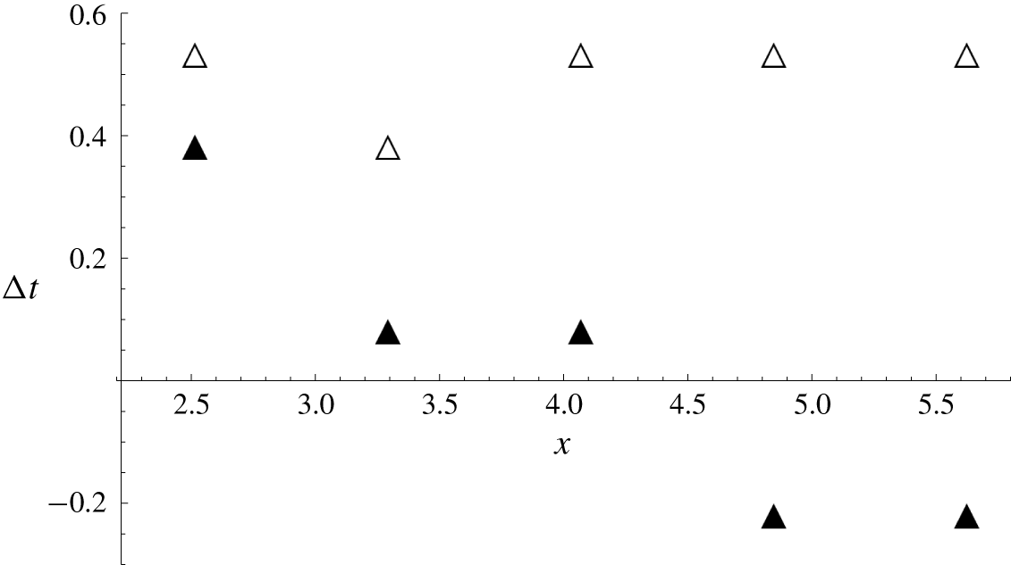
The spatial wave profile changes as the breaking proceeds. Figure 18 shows the time lags in arrival of the wave crest at the centreline of the sill  $y=0$ and the edge of the sill
 $y=4.26$ in comparison with the offshore ambient wave crest at
 $y=18$. The time lag between the crests at the edge of the sill
 $y=4.26$ and
 $y=18$ essentially remains constant. On the other hand, the time difference at the centre of the sill becomes progressively smaller as the wave breaking progresses, and eventually the breaking wave crest passes ahead of the ambient wave crest in the deeper water depth (
 $h_{0}=5~\text{cm}$). When the results shown in figure 18 are interpreted, it must be noted that the temporal resolution of the LIF technique we used was
 $1/125$ seconds, which is
 $\unicode[STIX]{x0394}t=0.130$ in normalized time.
Time lag in the arrival times of the wave crest between the offshore location ( $y=$ 18) and at the centre of the sill (
 $y=0$), ▴; between the offshore location (
 $y=18$) and at the edge of the sill (
 $y=4.26$), ▵.

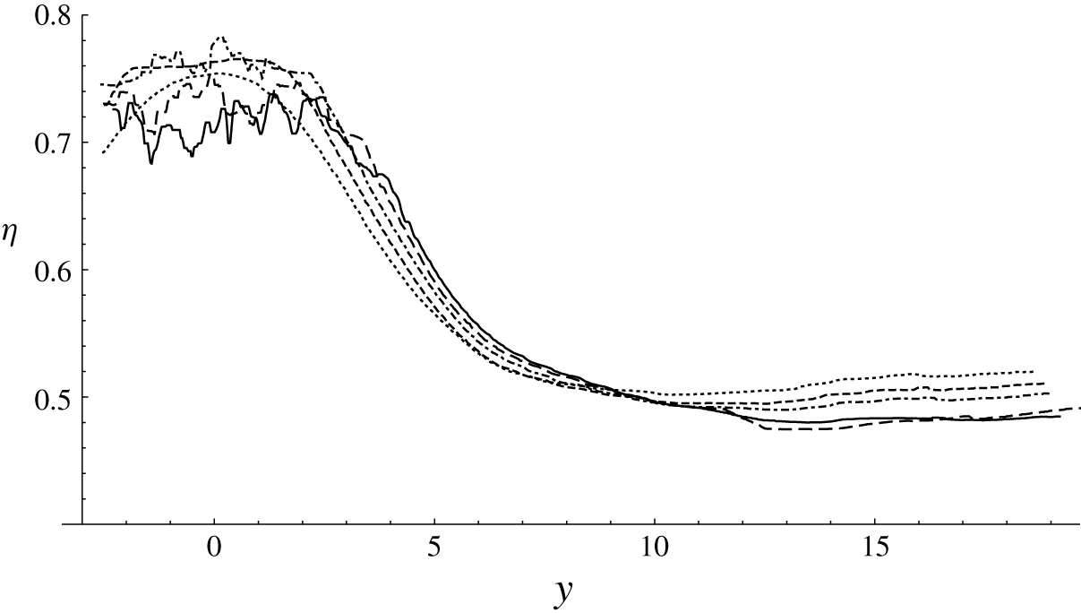
The maximum water-surface profile in the direction lateral to the wave propagation,  $y$ direction. The centreline of the sill is at
 $y=0$, and the edge of the sill is located at
 $y=4.26$. Solid line,
 $x=53.6$; long dashed line,
 $x=46.9$; dash-dot line,
 $x=40.3$; short dashed line,
 $x=33.5$; dotted line,
 $x=26.6$.

Figure 19 shows the profiles of the maximum water-surface elevation (i.e. the amplitude profiles) in the lateral direction at  $x=26.6$, 33.5, 40.3, 46.9 and 53.6. Several features that appear in the figure are worth noting. First, prior to the onset of breaking at
 $x=26.6$, the lateral amplitude profile is smooth across the sill, having a distinct global maximum at the centre of the sill. At the onset of breaking (
 $y=33.5$), no obvious irregularity has been developed yet in the amplitude profile, but the crest on the sill increases in both elevation and breadth, and its shape across the sill becomes flattened (a top-hat shape). Once wave breaking commences, the crest shape becomes irregular and further broadens towards offshore. While the wave amplitude decreases due to energy dissipation, the amplitude continues to grow in the area near the edge of the sill. The maximum wave amplitude at the edge of the sill (
 $y=4.26$) is
 $a=0.595$ at
 $x=3.17$, 0.608 at
 $x=33.5$, 0.622 at
 $x=40.3$, 0.635 at
 $x=46.9$ and 0.645 at
 $x=53.6$. Perhaps more important, the water-surface slope facing the
 $y$ direction becomes progressively steeper. It is noted that similar behaviour was reported by Li et al. (Reference Li, Yeh and Kodama2011) for their laboratory experiments on the breaking of a Mach reflection, which is also a three-dimensional wave-breaking phenomenon in shallow water.
So far, the results of wave breaking presented here are limited to the cases for one specific sill. As we demonstrated in § 4, solitary-wave response to a longitudinal sill is quite different depending on its breadth, even if the depth is kept constant. Therefore it is likely that the breaking behaviour differs depending upon the breadth of the sill.
6 Summary and conclusions
The response of a solitary wave to a local disturbance of a rectangular-shaped sill oriented in the direction of wave propagation is found to be similar for waves of  $a_{i}=0.1$, 0.2, 0.3 and 0.4. Presentation of laboratory measurements for two representative cases (Case A:
 $a_{i}=0.3$ with
 $b=0.254$; Case B:
 $a_{i}=0.2$ with
 $b=0.3175$) shows four key features:
(i) initial wave amplification over the sill which later begins to decay gradually;
(ii) enhanced and continual decay in wave amplitude off of the sill;
(iii) continually increasing phase lag between the portion of the wave over the sill and the rest of the wave; and
(iv) emergence of a radiating wave off the side edge of the sill.
Even though the wave tank used in this study is large ( $182.5h_{0}\times 90h_{0}$ for Case B), the propagation domain is still not long enough to examine the long-term effects of the longitudinal sill.
Motivated by the findings from the laboratory experiments, numerical experiments are performed to extend the laboratory observations. The numerical model implemented is based on a higher-order pseudo-spectral method, which can accurately solve the full water-wave Euler equations for irrotational flows of inviscid fluids. The numerical method simulates the wave evolution influenced by the sill for a very long distance (or time) without viscous attenuation. Here, the effects of three different sills are examined numerically: narrow, moderate and wide breadths of the sill with all other conditions kept the same. The moderate-width sill is intended to be similar to but not exactly the same as the rectangular-shaped sill used in the laboratory experiment: this is necessary to avoid any numerical instabilities caused by the edges of the rectangular-shaped sill. Nonetheless, the numerical results qualitatively confirm the laboratory observations, and furthermore provide the long-time process of the wave transformation. The results for all three sills (narrow, moderate and wide) show that the wave amplitude over the sill initially experiences a sharp increase before starting to decrease. For the narrow sill, the attenuation of the ambient wave is slower than the rate of viscous attenuation. The phase difference between the ambient wave and the wave on the sill approaches a nearly uniform state, indicating that the wave is gradually attenuated with its quasi-steady formation. This is not the case for the moderate- and wide-sill situations. The ambient amplitude attenuates at a rate similar to the viscous attenuation. The phase lag associated with the moderate and wide sills continually increases without a sign of reaching any equilibrium or quasi-steady state. The phase lag creates radiating waves at the side edges of the sill; the longitudinally placed submerged sill is a source of energy radiation. Consequently, long-term wave propagation over a longitudinal sill results in substantial attenuation of the solitary wave and continual deformation in wave pattern. The numerical simulation indicates that the continual energy radiation leads to the complete annihilation of the solitary wave in a very long wave tank.
We also performed laboratory experiments for the cases that induce wave breaking on the sill, and found that the maximum wave height prior to the onset of breaking  $a_{max}=0.759$ is smaller than the maximum height
 $a_{max}=0.827$ of the plain solitary wave reported by Longuet-Higgins & Fenton (Reference Longuet-Higgins and Fenton1974). This result is opposite to the maximum wave amplitude associated with the Mach reflection of a solitary wave
 $a_{max}=0.910$ reported by Li et al. (Reference Li, Yeh and Kodama2011). The low maximum wave amplitude must be caused by the presence of the sill; the leading flow under the solitary wave must be disturbed by the rectangular-shaped sill, causing flow separation at the salient edges of the sill. This disturbance triggers the early onset of breaking, although this is a conjecture because the detailed flow field was not measured. It must be noted that the breaking observed in the present experiment did not induce any overturning of the water surface nor air-bubble entrainment; instead, the breaking is characterized as the formation of parasitic capillary waves on the front face of the wave. After incipient breaking at the centre of the sill (
 $y=0$), the breaking broadens outwards, covering its breaking crest over the sill breadth. The water-surface elevation at the edge of the sill grows, resulting in a steeper water surface in the lateral direction. Meanwhile, the breaking wave crest progressively advances faster, and eventually exceeds the ambient wave crest. Also observed is the formation of a wake-like gravity–capillary wavetrain behind the breaking wave crest emitting outwards from the sill.
In summary, a submerged broad sill running parallel to the propagation of a solitary wave induces wave radiation from the edge of the sill; hence the wave energy radiates and the amplitude attenuates at a rate comparable to (or even greater than) that of the viscous effect. Furthermore, a solitary wave tends to break on the sill much earlier than the stage of a solitary wave on a horizontal bed; the presence of the sill induces a disturbance which triggers early wave breaking. Consequently, there is a potential to consider a submerged sill oriented in the direction of wave propagation as an effective wave-energy attenuator for localized waves that can be represented by solitary waves. This may not be the case for a submerged sill oriented perpendicular to the wave propagation, as we reported in Part 1. In some cases, solitary waves passing over such sills are not affected at all or very slightly, unless wave breaking is induced over the sill. Even if wave breaking occurs over the sill, the wave is recovered immediately after passing over the sill.
Acknowledgements
This work was partially supported by the US National Science Foundation (OCE-1830024). Note that all the data presented in the paper are available upon request from the corresponding author.
Appendix A
The following is a description of the algorithm based on the work by Dommermuth & Yue (Reference Dommermuth and Yue1987) in order to solve Euler’s formulation via the pseudo-spectral method. We consider a homogeneous, inviscid, irrotational flow in which the mathematical description is given by the Zakharov–Craig–Sulem formulation (Craig & Sulem Reference Craig and Sulem1993; Zakharov Reference Zakharov1968) of the full water-wave equations in the three-dimensional domain:
 $$\begin{eqnarray}\begin{array}{@{}cc@{}}\unicode[STIX]{x1D6F7}_{xx}+\unicode[STIX]{x1D6F7}_{yy}+\unicode[STIX]{x1D6F7}_{zz}=0 & \text{for }-1+\unicode[STIX]{x1D701}\leqslant z\leqslant \unicode[STIX]{x1D702},\\ \unicode[STIX]{x1D735}\unicode[STIX]{x1D6F7}\boldsymbol{\cdot }\unicode[STIX]{x1D735}\unicode[STIX]{x1D701}-\unicode[STIX]{x1D6F7}_{z}=0 & \text{at }z=-1+\unicode[STIX]{x1D701},\\ \left.\begin{array}{@{}c@{}}\displaystyle \unicode[STIX]{x1D702}_{t}+\unicode[STIX]{x1D735}\unicode[STIX]{x1D6F7}^{S}\boldsymbol{\cdot }\unicode[STIX]{x1D735}\unicode[STIX]{x1D702}-(1+|\unicode[STIX]{x1D735}\unicode[STIX]{x1D702}|^{2})\unicode[STIX]{x1D6F7}_{z}=0\\ \displaystyle \unicode[STIX]{x1D6F7}_{t}^{S}+\unicode[STIX]{x1D702}+{\textstyle \frac{1}{2}}|\unicode[STIX]{x1D735}\unicode[STIX]{x1D6F7}^{S}|^{2}-{\textstyle \frac{1}{2}}(1+|\unicode[STIX]{x1D735}\unicode[STIX]{x1D702}|^{2})\unicode[STIX]{x1D6F7}_{z}^{2}=0\end{array}\right\} & \text{at }z=\unicode[STIX]{x1D702},\end{array}\end{eqnarray}$$
where  $\unicode[STIX]{x1D6F7}(\boldsymbol{x},z,t)$ is the velocity potential,
 $\unicode[STIX]{x1D701}(\boldsymbol{x})$ is the bed variation about the mean horizontal bathymetry,
 $\unicode[STIX]{x1D702}(\boldsymbol{x},t)$ is the surface displacement,
 $\unicode[STIX]{x1D6F7}^{S}(\boldsymbol{x},t)\equiv \unicode[STIX]{x1D6F7}(\boldsymbol{x},t,z=\unicode[STIX]{x1D702}(\boldsymbol{x},t))$ is the velocity potential at the free surface,
 $\unicode[STIX]{x1D735}=(\unicode[STIX]{x2202}/\unicode[STIX]{x2202}x,\unicode[STIX]{x2202}/\unicode[STIX]{x2202}y)$ represents the horizontal gradient and
 $\boldsymbol{x}=(x,y)$. Note that, in this formulation,
 $z$ originates at the mean water surface and points upward. The velocity potential is expressed as an asymptotic expansion:
 $$\begin{eqnarray}\unicode[STIX]{x1D6F7}(\boldsymbol{x},z,t)=\mathop{\sum }_{m=1}^{M}\unicode[STIX]{x1D719}^{(m)}(\boldsymbol{x},z,t),\end{eqnarray}$$
in which the superscript  $(m)$ denotes that the term is of the order
 $O\sim (a_{i}^{m})$, where
 $a_{i}$ is a small parameter which represents the nonlinearity effect. Each perturbation term is expressed as a two-term expansion
 $\unicode[STIX]{x1D719}^{(m)}=A^{(m)}+B^{(m)}$ in which
 $$\begin{eqnarray}A^{(m)}(\boldsymbol{x},z,t)=\mathop{\sum }_{p=-\infty }^{\infty }\mathop{\sum }_{q=-\infty }^{\infty }A_{p,q}^{(m)}(t)\,\frac{\cosh |\unicode[STIX]{x1D73F}_{p,q}|(z+1)}{\cosh |\unicode[STIX]{x1D73F}_{p,q}|}\,\text{e}^{\text{i}\unicode[STIX]{x1D73F}_{p,q}\cdot \boldsymbol{x}}\end{eqnarray}$$
and
 $$\begin{eqnarray}B^{(m)}(\boldsymbol{x},z,t)=\mathop{\sum }_{p=-\infty }^{\infty }\mathop{\sum }_{q=-\infty }^{\infty }B_{p,q}^{(m)}(t)\,\frac{\sinh |\unicode[STIX]{x1D73F}_{p,q}|z}{|\unicode[STIX]{x1D73F}_{p,q}|\cosh |\unicode[STIX]{x1D73F}_{p,q}|}\,\text{e}^{\text{i}\unicode[STIX]{x1D73F}_{p,q}\cdot \boldsymbol{x}}.\end{eqnarray}$$
The basis functions  $A^{(m)}$ and
 $B^{(m)}$ satisfy Laplace’s equation and
 $A^{(m)}$ satisfies the Neumann boundary condition at
 $z=-1$ and
 $B^{(m)}$ satisfies the Dirichlet boundary conditon at
 $z=0$. In (A 3) and (A 4),
 $\unicode[STIX]{x1D73F}_{p,q}=(p\unicode[STIX]{x03C0}/L_{x},q\unicode[STIX]{x03C0}/L_{y})$ is the wavenumber vector, where
 $L_{x}$ and
 $L_{y}$ are the length and width of the domain, respectively. The magnitude of the wavenumber vector is
 $|\unicode[STIX]{x1D73F}_{p,q}|=\sqrt{(p\unicode[STIX]{x03C0}/L_{x})^{2}+(q\unicode[STIX]{x03C0}/L_{y})^{2}}$, and
 $\text{i}=\sqrt{-1}$.
A four-stage Runge–Kutta method (e.g. Boyce, DiPrima & Meade Reference Boyce, Diprima and Meade1992) is used to numerically time-integrate the evolution equations:
 $$\begin{eqnarray}\left.\begin{array}{@{}c@{}}\displaystyle \unicode[STIX]{x1D702}_{t}=-\unicode[STIX]{x1D735}\unicode[STIX]{x1D6F7}^{S}\boldsymbol{\cdot }\unicode[STIX]{x1D735}\unicode[STIX]{x1D702}+(1+|\unicode[STIX]{x1D735}\unicode[STIX]{x1D702}|^{2})\unicode[STIX]{x1D6F7}_{z},\\ \unicode[STIX]{x1D6F7}_{t}^{S}=\displaystyle -\unicode[STIX]{x1D702}-{\textstyle \frac{1}{2}}|\unicode[STIX]{x1D735}\unicode[STIX]{x1D6F7}^{S}|^{2}+{\textstyle \frac{1}{2}}(1+|\unicode[STIX]{x1D735}\unicode[STIX]{x1D702}|^{2})\unicode[STIX]{x1D6F7}_{z}^{2},\end{array}\right\}\end{eqnarray}$$
on  $z=\unicode[STIX]{x1D702}$. The horizontal gradient is calculated by the algebraic derivative by making use of the fast Fourier transform. In order to calculate the vertical velocity
 $\unicode[STIX]{x1D6F7}_{z}$ at the water surface, we must first calculate the degrees of freedom of the basis functions. In other words, we need to use the Fourier transform to determine the coefficients
 $A_{p,q}^{(m)}(t)$ and
 $B_{p,q}^{(m)}(t)$. This is achielved by expanding the velocity potential at the mean water surface as well as at the bottom bed boundary. At the water surface
 $$\begin{eqnarray}\unicode[STIX]{x1D6F7}^{S}(\boldsymbol{x},t)=\mathop{\sum }_{m=1}^{M}\mathop{\sum }_{k=0}^{M-m}\frac{\unicode[STIX]{x1D702}^{k}}{k!}\frac{\unicode[STIX]{x2202}^{k}\unicode[STIX]{x1D719}^{(m)}}{\unicode[STIX]{x2202}z^{k}}\bigg|_{(\boldsymbol{x},z=0,t)},\end{eqnarray}$$
and we use  $M=5$ so that after expanding out the sum and equating terms of like order we have
 $$\begin{eqnarray}\left.\begin{array}{@{}c@{}}A^{(1)}=\unicode[STIX]{x1D6F7}^{S},\\ A^{(2)}=-\unicode[STIX]{x1D702}(A^{(1)}+B^{(1)})_{z},\\[5.0pt] \displaystyle A^{(3)}=-\unicode[STIX]{x1D702}(A^{(2)}+B^{(2)})_{z}-{\displaystyle \frac{\unicode[STIX]{x1D702}^{2}}{2!}}A_{zz}^{(1)},\\[7.0pt] \displaystyle A^{(4)}=-\unicode[STIX]{x1D702}(A^{(3)}+B^{(3)})_{z}-{\displaystyle \frac{\unicode[STIX]{x1D702}^{2}}{2!}}A_{zz}^{(2)}-{\displaystyle \frac{\unicode[STIX]{x1D702}^{3}}{3!}}(A^{(1)}+B^{(1)})_{zzz},\\[5.0pt] \displaystyle A^{(5)}=-\unicode[STIX]{x1D702}(A^{(4)}+B^{(4)})_{z}-{\displaystyle \frac{\unicode[STIX]{x1D702}^{2}}{2!}}A_{zz}^{(3)}-{\displaystyle \frac{\unicode[STIX]{x1D702}^{3}}{3!}}(A^{(2)}+B^{(2)})_{zzz}-{\displaystyle \frac{\unicode[STIX]{x1D702}^{4}}{4!}}A_{zzzz}^{(1)},\end{array}\right\}\end{eqnarray}$$
all on  $z=0$. The coefficients of (A 3) and (A 4) can then be found from the Fourier transform once the
 $B^{(m)}$ terms are known. Therefore, we continue in a similar fashion by expanding the velocity potential about the bottom bed boundary:
 $$\begin{eqnarray}\unicode[STIX]{x1D6F7}(\boldsymbol{x},z,t)=\mathop{\sum }_{m=1}^{M}\mathop{\sum }_{k=0}^{M-m}\frac{(z+1)^{k}}{k!}\frac{\unicode[STIX]{x2202}^{k}\unicode[STIX]{x1D719}^{(m)}}{\unicode[STIX]{x2202}z^{k}}\bigg|_{(\boldsymbol{x},z=-1,t)}.\end{eqnarray}$$
We then substitute (A 8) into the second line of (A 1) and equate terms of like order assuming that  $\unicode[STIX]{x1D701}$ and its derivatives are also of the order of
 $a_{i}$. After equating terms of like order we have
 $$\begin{eqnarray}\left.\begin{array}{@{}c@{}}B_{z}^{(1)}=0,\\[5.0pt] B_{z}^{(2)}=\unicode[STIX]{x1D735}\unicode[STIX]{x1D701}\boldsymbol{\cdot }\unicode[STIX]{x1D735}A^{(1)}-\unicode[STIX]{x1D701}A_{zz}^{(1)},\\[5.0pt] B_{z}^{(3)}=\unicode[STIX]{x1D735}\unicode[STIX]{x1D701}\boldsymbol{\cdot }\unicode[STIX]{x1D735}(A^{(2)}+B^{(2)})-\unicode[STIX]{x1D701}(A_{zz}^{(2)}+B_{zz}^{(2)}),\\[5.0pt] \displaystyle B_{z}^{(4)}=\unicode[STIX]{x1D735}\unicode[STIX]{x1D701}\boldsymbol{\cdot }(\unicode[STIX]{x1D735}A^{(3)}+\unicode[STIX]{x1D735}B^{(3)}+\unicode[STIX]{x1D701}\unicode[STIX]{x1D735}B_{z}^{(2)}+{\displaystyle \frac{\unicode[STIX]{x1D701}^{2}}{2!}}\unicode[STIX]{x1D735}A_{zz}^{(1)})\\[5.0pt] -\unicode[STIX]{x1D701}(A_{zz}^{(3)}+B_{zz}^{(3)}+{\displaystyle \frac{\unicode[STIX]{x1D701}}{2!}}B_{zzz}^{(2)}+{\displaystyle \frac{\unicode[STIX]{x1D701}^{2}}{3!}}A_{zzzz}^{(1)}),\\[5.0pt] \displaystyle B_{z}^{(5)}=\unicode[STIX]{x1D735}\unicode[STIX]{x1D701}\boldsymbol{\cdot }(\unicode[STIX]{x1D735}A^{(4)}+\unicode[STIX]{x1D735}B^{(4)}+\unicode[STIX]{x1D701}\unicode[STIX]{x1D735}B_{z}^{(3)}+{\displaystyle \frac{\unicode[STIX]{x1D701}^{2}}{2!}}\unicode[STIX]{x1D735}A_{zz}^{(2)}+{\displaystyle \frac{\unicode[STIX]{x1D701}^{2}}{2!}}\unicode[STIX]{x1D735}B_{zz}^{(2)})\\[5.0pt] -\unicode[STIX]{x1D701}(A_{zz}^{(4)}+B_{zz}^{(4)}+{\displaystyle \frac{\unicode[STIX]{x1D701}}{2!}}B_{zzz}^{(3)}+\displaystyle {\displaystyle \frac{\unicode[STIX]{x1D701}^{2}}{3!}}A_{zzzz}^{(2)}+{\displaystyle \frac{\unicode[STIX]{x1D701}^{2}}{3!}}B_{zzzz}^{(2)}),\end{array}\right\}\end{eqnarray}$$
all on  $z=-1$. From (A 4) we see with the use of the Fourier transform that the degrees of freedom
 $B_{p,q}^{(1)}(t)$ are all zero and therefore
 $B^{(1)}$ is zero for all
 $t$. Therefore
 $B^{(1)}$ may be omitted from (A 7) as well. From the recurrence relations established in (A 7) and (A 9) we can determine all of the degrees of freedom. After the degrees of freedom are determined the vertical velocity at the water surface can be calculated:
 $$\begin{eqnarray}\unicode[STIX]{x1D6F7}_{z}(\boldsymbol{x},z=\unicode[STIX]{x1D702},t)=\mathop{\sum }_{m=1}^{M}\mathop{\sum }_{k=0}^{M-m}\frac{\unicode[STIX]{x1D702}^{k}}{k!}\frac{\unicode[STIX]{x2202}^{k+1}\unicode[STIX]{x1D719}^{(m)}}{\unicode[STIX]{x2202}z^{k+1}}\bigg|_{(\boldsymbol{x},z=0,t)}.\end{eqnarray}$$
Then, the solution is completely determined once the initial conditions for  $\unicode[STIX]{x1D702}$ and
 $\unicode[STIX]{x1D6F7}^{S}$ are prescribed.
In order to extend the simulation beyond the original domain, we implement a patching trick where a translation is performed on the data once the leading crest of the solitary wave nears sufficiently close to the end of the domain. The translation of the data is given by  $\unicode[STIX]{x1D6F7}_{new}^{S}(x,y,t)=\unicode[STIX]{x1D6F7}^{S}(x-X_{new},y,t)$ and
 $\unicode[STIX]{x1D702}_{new}(x,y,t)=\unicode[STIX]{x1D702}(x-X_{new},y,t)$, where
 $\unicode[STIX]{x1D6F7}_{new}^{S}$ and
 $\unicode[STIX]{x1D702}_{new}$ are the translated values of the water-surface velocity potential and surface displacement, respectively, and
 $X_{new}=374.6$. This process was performed at times
 $t=1005.4$, 1346.8 and 1722.7 in order to extend the simulation. This translation operation has also been successfully implemented to simulate the Mach reflection of a solitary wave by Jia (Reference Jia2014) and Knowles & Yeh (Reference Knowles and Yeh2019). Furthermore, the pseudo-spectral method has been adapted to a varying one-dimensional bathymetry to study the shoaling of solitary waves propagating over plane beaches (Knowles & Yeh Reference Knowles and Yeh2018). This pseudo-spectral method was also verified in experiments by Gouin, Ducrozet & Ferrant (Reference Gouin, Ducrozet and Ferrant2016) for two-dimensional bathymetry.
For implementing the foregoing numerical algorithm, the following three sill models are used in the numerical experiments: ‘narrow’, ‘moderate’ and ‘wide’. The sill in terms of the bed elevation  $\unicode[STIX]{x1D701}(x,y)$ for the ‘narrow’ case is represented by
 $$\begin{eqnarray}\unicode[STIX]{x1D701}(x,y)=\frac{b}{2}(1+\tanh k_{x}x)\text{e}^{-(k_{y}[y-y_{0}])^{2}},\end{eqnarray}$$
where  $k_{x}$ and
 $k_{y}$ are measures of the steepness of the sill in the
 $x$ and
 $y$ directions, respectively. To approximate the sill with a flat top, we prescribe the following configuration for the sill for the ‘moderate’ and ‘wide’ cases:
 $$\begin{eqnarray}\unicode[STIX]{x1D701}(x,y)=\frac{b}{4}(1+\tanh k_{x}x)(1-\tanh k_{y}[y-y_{0}]),\end{eqnarray}$$
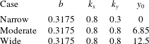
where parameters for the different bathymetries are presented in table 1. The cross-sections of the different sills adopted in the numerical calculations are depicted in figure 9.