1 Introduction
Water wave dynamics in coastal regions, where surface waves are affected by depth variations, is a problem of great interest from the environmental point of view as well as due to its mathematical diversity (formulation, theory and computation). It is a long-lasting source of problems, with still many challenges. The problems are very complex, in particular in the presence of a bottom topography. Some of these problems are related to the Euler (potential theory) equations, while others to its reduced models, such as the weakly nonlinear, weakly dispersive Boussinesq system. The topography may come into the problem in a geometric fashion as a variable boundary or as a variable coefficient (in an algebraic form). Inclusion of topographic features, in either way, is a relevant physical ingredient of current research interest and has been addressed from the analysis viewpoint, as well as regarding computational modelling and related issues.
Non-local water wave formulations make use of the harmonic properties of the velocity potential. In particular for two-dimensional incompressible, irrotational flows, a variety of non-local boundary integral formulations have been used. The literature is abundant and accessible, and therefore we cite only a few articles (Milewski Reference Milewski1998; Choi & Milewski Reference Choi and Milewski2003; Guyenne & Nicholls Reference Guyenne and Nicholls2005; Deconinck & Oliveras Reference Deconinck and Oliveras2011; Vasan & Deconinck Reference Vasan and Deconinck2013; Wilkening & Vasan Reference Wilkening and Vasan2015), which should be good sources of additional references. More recently non-local formulations through the Dirichlet-to-Neumann (DtN) operator have become popular, both theoretically and numerically. The operator collapses all information onto the free surface. The dimension of the problem is reduced. For example, the dynamics in a three-dimensional fluid body is reduced to computing only with information along the two-dimensional free surface.
Taking the one-dimensional case for simplicity, the non-local operators here considered arise in the form of Fourier integrals:
 $$\begin{eqnarray}\displaystyle & \displaystyle F[f](x)=\iint \text{e}^{\text{i}k(x-x^{\prime })}w(k)f(x^{\prime })\,\text{d}x^{\prime }\,\text{d}k. & \displaystyle\end{eqnarray}$$
The Fourier integral operator
 $F$
acts on
 $f$
, where
 $w(k)$
is the Fourier multiplier (symbol). If the multiplier is a polynomial in
 $k$
, then
 $F$
is a differential operator. Owing to the presence of the topography in the present formulation, the symbol will be
 $x$
-dependent.
An early derivation is due to Milewski (Reference Milewski1998), where the author proposes a Fourier integral equation for the water wave problem. Milewski uses the two (linearly independent) hyperbolic functions for harmonically extending boundary data into the fluid domain. By expanding the symbol appropriately, to leading order, the Fourier integral characterizes a differential operator. Milewski then recovers the standard long-wave (asymptotic) equations such as the Benny–Luke, the Boussinesq and the Korteweg–de Vries (KdV) equations. His models incorporate topographical effects through variable coefficients and forcing terms. These approximations are valid when the topographical variations are slowly varying with respect to the wave field.
Recently the non-local formulation proposed by Ablowitz, Fokas & Musslimani (Reference Ablowitz, Fokas and Musslimani2006) has called attention to an alternative water wave model. The authors derive a set of global relations that couple free surface equations together with Fourier components, namely, the vertical harmonic extension of Fourier modes given at the free surface. These Fourier components are expressed through hyperbolic functions and, when expanded, give rise to differential operators defined as powers of the wavenumber
 $k$
in Fourier space. Hereafter the formulation proposed in Ablowitz et al. (Reference Ablowitz, Fokas and Musslimani2006) will be called the AFM formulation. Deconinck & Oliveras (Reference Deconinck and Oliveras2011) used the AFM formulation to compute periodic travelling wave solutions. Their work represents one of the first steps towards the use of the AFM (non-local) equations in the numerical simulation of water waves. They studied wave stability, showing that it is possible to solve the non-local equations accurately. The AFM formulation has been considered in other water wave problems, as for example by Haut & Ablowitz (Reference Haut and Ablowitz2009) for internal waves and by Ashton & Fokas (Reference Ashton and Fokas2011) for waves with vorticity. Vasan & Deconinck (Reference Vasan and Deconinck2013) made a contribution in the context of time-dependent AFM simulations, in the presence of topography. Their goal was to recover the bottom profile from surface measurements.
A very detailed comparison between five different DtN formulations is provided by Wilkening & Vasan (Reference Wilkening and Vasan2015). Among other things, they consider the AFM method as well as their dual formulation, called the AFM
 $^{\ast }$
method. Wilkening & Vasan (Reference Wilkening and Vasan2015) showed that the Craig–Sulem series expansions, the AFM and AFM
 $^{\ast }$
methods require high-precision intermediate calculations to achieve double-precision accuracy, whereas boundary integral methods and transformed field expansion methods do not suffer significant loss of digits since they employ well-conditioned representations of the solution of the Laplace equation. The formulation found in Milewski (Reference Milewski1998), Craig et al. (Reference Craig, Guyenne, Nicholls and Sulem2005) is namely an AFM
 $^{\ast }$
method. Our formulation follows the line of Milewski (Reference Milewski1998) together with a Galerkin method, leading to accurate results in the presence of highly variable topographies, including in three dimensions.
Non-local equations in the presence of topography also appear in the work of Craig et al. (Reference Craig, Guyenne, Nicholls and Sulem2005). The authors define the respective Fourier multiplier operators, as will be briefly described. Having in mind their work from Craig & Sulem (Reference Craig and Sulem1993), they show that the topographical contribution is given by an extra term in the Fourier representation. For simplicity, consider the Fourier multiplier operator notation in two dimensions, ignoring for a moment the time dependence of the potential:
 $$\begin{eqnarray}\displaystyle & \displaystyle \unicode[STIX]{x1D719}(x,z)=\iint \text{e}^{\text{i}k(x-x^{\prime })}{\displaystyle \frac{\cosh (k(z+h))}{\cosh (kh)}}q(x^{\prime })\,\text{d}x^{\prime }\,\text{d}k\equiv {\displaystyle \frac{\cosh ((z+h)D)}{\cosh (hD)}}q(x), & \displaystyle\end{eqnarray}$$
where
 $D\equiv \text{i}\unicode[STIX]{x2202}x$
. It is easy to see, by separation of variables, that the Fourier integral representation of the potential satisfies Laplace’s equation in a two-dimensional strip, of height
 $h$
, together with the following boundary conditions: a homogeneous Neumann condition at the bottom
 $z=-h$
, and a Dirichlet condition
 $\unicode[STIX]{x1D719}(x,0)=q(x)$
at the top boundary
 $z=0$
. In three dimensions the notation becomes
 $D=(D_{1},D_{2})^{\text{T}}\equiv \text{i}(\unicode[STIX]{x2202}x,\unicode[STIX]{x2202}y)^{\text{T}}$
. In the presence of a bottom topography
 $z=-(h+H(\boldsymbol{x}))$
, the Fourier operator has an additional term in order to account for the presence of the topography
 $H(\boldsymbol{x})$
,
 $\boldsymbol{x}=(x,y)$
. Craig et al. (Reference Craig, Guyenne, Nicholls and Sulem2005) present their ansatz by expressing the velocity potential as
 $$\begin{eqnarray}\displaystyle & \displaystyle \unicode[STIX]{x1D719}(\boldsymbol{x},z)={\displaystyle \frac{\cosh ((z+h)|D|)}{\cosh (h|D|)}}q(\boldsymbol{x})+\sinh (z|D|)L(H)q(\boldsymbol{x}). & \displaystyle\end{eqnarray}$$
The Fourier integral operator
 $L(H)$
is defined implicitly (see equation (2.23) and the appendix in Craig et al. (Reference Craig, Guyenne, Nicholls and Sulem2005)) through a relation that contains two other topography-dependent Fourier integral operators,
 $A(H)$
and
 $B(H)$
:
 $$\begin{eqnarray}\displaystyle \left.\begin{array}{@{}l@{}}A(H)=\sinh (H(\boldsymbol{x})|D|)\,\text{sech}(h|D|),\\ C(H)=\cosh ((H(\boldsymbol{x})-h)|D|),\quad \text{with }B(H)=C(H)^{-1}.\end{array}\right\} & & \displaystyle\end{eqnarray}$$
In their appendix, assuming that the bottom topography is small with respect to the reference depth, Craig et al. (Reference Craig, Guyenne, Nicholls and Sulem2005) give a series expansion for the topographical part of the operator. The authors mention that when the topography profile is
 $O(1)$
, a Taylor expansion is not what one should seek. Also, in the conclusions, that: ‘Preliminary numerical results appear in Guyenne & Nicholls (Reference Guyenne and Nicholls2005). More in-depth numerical computations constitute a substantial contribution in their own right ….’ Guyenne & Nicholls (Reference Guyenne and Nicholls2005) considered expansions for the wave and the bottom topography operators. Their model was used to simulate the shoaling of solitary waves propagating over inclined planes. High-frequency instabilities were reported and treated with a low-pass filter for the velocity potential and wave elevation functions. However, it is not clear what is exactly the source of the instability. As reported by the authors, it could be due to the ill-posedness of the truncation process that arises in the wave expansion, as recently investigated by Ambrose, Bona & Nicholls (Reference Ambrose, Bona and Nicholls2013), or it could be due to the topographic operator component.
In the present work we focus on the topographic component of the Fourier integral operator, which is computed numerically as a matrix decomposition, along the lines mentioned above. Our ansatz for the topographic component is different from that displayed in (1.3) and follows the simpler expression given by Milewski (Reference Milewski1998). We take into account highly variable non-smooth topographies, which inhibits the use of a series expansion. A physically motivated Galerkin method acts only on low frequencies of the topographic component of the DtN operator, keeping only modes that can indeed interact with the bottom variations. The velocity potential
 $\unicode[STIX]{x1D719}$
and the wave elevation
 $\unicode[STIX]{x1D702}$
are not filtered. Hence with the ingredients we considered, the topographic formulation, along the lines of Milewski (Reference Milewski1998) and Craig et al. (Reference Craig, Guyenne, Nicholls and Sulem2005), performed very well for a range of non-trivial problems. These include large-amplitude rapidly varying topographies, as well as three-dimensional landscapes, where the non-local formulation had not been tested before. Three-dimensional simulations can be very time-consuming and the Galerkin method played an important role.
A recent work by Cathala (Reference Cathala2016) regards the analysis of two-dimensional computations with the formulation provided by Craig et al. (Reference Craig, Guyenne, Nicholls and Sulem2005). Cathala takes a second-order expansion in both the wave and the topographic operators. Cathala (Reference Cathala2016) considers, in particular, the case of polygonal topographies: a submerged step that rises up to half the depth of the channel. He compares his result with that of Nachbin (Reference Nachbin2003) and obtains a satisfactory comparison. Based on conformal mapping, Nachbin considers a Boussinesq system in the presence of a polygonal topography.
In another recent work, Vargas-Magaña & Panayotaros (Reference Vargas-Magaña and Panayotaros2016) use the series expansion of Craig et al. (Reference Craig, Guyenne, Nicholls and Sulem2005) and deduce a Whitham–Boussinesq model with topography. The numerical modelling is two-dimensional. Their approach simplifies the contribution of the topographic operators by introducing a simpler non-local equation. They show that their operator captures the right asymptotic behaviour for high wavenumbers. Their numerical scheme also uses a Galerkin approximation similar to ours and is tested for a smooth submerged Gaussian mound.
In summary, the technique presented here is validated for solving non-trivial linear water wave problems in three dimensions. The method uses a non-local formulation that reduces the evolution system to a two-dimensional surface. As our main goal, a DtN operator is constructed in the presence of large-amplitude, non-smooth topographies retaining, along the two-dimensional surface, information from the vertical flow structure. A Galerkin method in Fourier space is used to make the topographic component of the DtN operator amenable to accurate computations.
This article is organized as follows. In § 2 we introduce the potential theory equations and the associated elliptic boundary value problem for constructing the DtN operator over a flat bottom. Section 3 considers the variable-depth non-local formulation and the associated decomposition for the three-dimensional DtN operator. Section 4 presents several water wave simulations in two and three dimensions. The conclusions are given in § 5.
2 Governing equations
2.1 Water wave equations
Potential theory is the classical hydrodynamic model that describes the motion of an incompressible, irrotational flow under the action of gravity (Whitham Reference Whitham1999):
 $$\begin{eqnarray}\displaystyle & \displaystyle \unicode[STIX]{x1D719}_{xx}+\unicode[STIX]{x1D719}_{yy}+\unicode[STIX]{x1D719}_{zz}=0,\quad \text{in}\;-\!b(\boldsymbol{x})<z<\unicode[STIX]{x1D702}(\boldsymbol{x},t), & \displaystyle\end{eqnarray}$$
 $$\begin{eqnarray}\displaystyle & \displaystyle \unicode[STIX]{x1D719}_{z}-\unicode[STIX]{x1D719}_{x}b_{x}-\unicode[STIX]{x1D719}_{y}b_{y}=0,\quad \text{on }z=-b(\boldsymbol{x}), & \displaystyle\end{eqnarray}$$
 $$\begin{eqnarray}\displaystyle & \displaystyle \unicode[STIX]{x1D702}_{t}+\unicode[STIX]{x1D719}_{x}\unicode[STIX]{x1D702}_{x}+\unicode[STIX]{x1D719}_{y}\unicode[STIX]{x1D702}_{y}-\unicode[STIX]{x1D719}_{z}=0,\quad \text{on }z=\unicode[STIX]{x1D702}(\boldsymbol{x},t), & \displaystyle\end{eqnarray}$$
 $$\begin{eqnarray}\displaystyle & \displaystyle \unicode[STIX]{x1D719}_{t}+g\unicode[STIX]{x1D702}+{\textstyle \frac{1}{2}}(\unicode[STIX]{x1D719}_{x}^{2}+\unicode[STIX]{x1D719}_{y}^{2}+\unicode[STIX]{x1D719}_{z}^{2})=0,\quad \text{on }z=\unicode[STIX]{x1D702}(\boldsymbol{x},t). & \displaystyle\end{eqnarray}$$
In these equations
 $\boldsymbol{x}=(x,y)$
denotes the horizontal variables,
 $g$
is the acceleration due to gravity,
 $\unicode[STIX]{x1D702}$
denotes the height of the surface wave,
 $\unicode[STIX]{x1D719}$
is the velocity potential of the fluid flow and finally
 $b$
denotes the impermeable bottom topography. We assume that
 $\unicode[STIX]{x1D702}$
,
 $\unicode[STIX]{x1D719}$
and its derivatives vanish at infinity.
The bottom of the fluid domain is described as
 $$\begin{eqnarray}\displaystyle & \displaystyle b(\boldsymbol{x})=h+H(\boldsymbol{x}), & \displaystyle\end{eqnarray}$$
where
 $h$
is a positive constant and the depth variation function
 $H$
is such that
 $$\begin{eqnarray}\displaystyle & \displaystyle -h<H(\boldsymbol{x}). & \displaystyle\end{eqnarray}$$
This restriction implies that no islands nor beaches are present in the fluid domain. But it allows for high-amplitude, non-smooth obstacles, as will be presented herein.
2.1.1 Non-dimensional form
It is customary to work with a non-dimensional form of the equations. This can be accomplished by replacing all the variables in equations (2.1)–(2.4) with primes and making the following substitutions:
 $$\begin{eqnarray}\displaystyle \left.\begin{array}{@{}l@{}}\displaystyle x^{\prime }=lx,\quad y^{\prime }=ly,\quad z^{\prime }=hz,\quad t^{\prime }={\displaystyle \frac{l}{\sqrt{gh}}}t,\\ \displaystyle \unicode[STIX]{x1D702}^{\prime }=a\unicode[STIX]{x1D702},\quad \unicode[STIX]{x1D719}^{\prime }=a\sqrt{gh}{\displaystyle \frac{l}{h}}\unicode[STIX]{x1D719},\quad H^{\prime }=hH.\end{array}\right\} & & \displaystyle\end{eqnarray}$$
In these new variables
 $l$
denotes a typical length scale for both horizontal directions,
 $h$
denotes a typical depth of the fluid domain,
 $a$
denotes a typical amplitude of the wave and
 $\sqrt{gh}$
is the typical speed of long waves propagating over an ocean of constant depth
 $h$
. The following dimensionless parameters arise:
 $\unicode[STIX]{x1D707}=h/l$
and
 $\unicode[STIX]{x1D700}=a/h$
.
The dimensionless equations are thus
 $$\begin{eqnarray}\displaystyle & \displaystyle \unicode[STIX]{x1D707}^{2}(\unicode[STIX]{x1D719}_{xx}+\unicode[STIX]{x1D719}_{yy})+\unicode[STIX]{x1D719}_{zz}=0,\quad \text{in }-(1+H(\boldsymbol{x}))<z<\unicode[STIX]{x1D700}\unicode[STIX]{x1D702}(\boldsymbol{x},t), & \displaystyle\end{eqnarray}$$
 $$\begin{eqnarray}\displaystyle & \displaystyle \unicode[STIX]{x1D719}_{z}-\unicode[STIX]{x1D707}^{2}(\unicode[STIX]{x1D719}_{x}H_{x}+\unicode[STIX]{x1D719}_{y}H_{y})=0,\quad \text{on }z=-(1+H(\boldsymbol{x})), & \displaystyle\end{eqnarray}$$
 $$\begin{eqnarray}\displaystyle & \displaystyle \unicode[STIX]{x1D702}_{t}+\unicode[STIX]{x1D700}(\unicode[STIX]{x1D719}_{x}\unicode[STIX]{x1D702}_{x}+\unicode[STIX]{x1D719}_{y}\unicode[STIX]{x1D702}_{y})-{\displaystyle \frac{1}{\unicode[STIX]{x1D707}^{2}}}\unicode[STIX]{x1D719}_{z}=0,\quad \text{on }z=\unicode[STIX]{x1D700}\unicode[STIX]{x1D702}(\boldsymbol{x},t), & \displaystyle\end{eqnarray}$$
 $$\begin{eqnarray}\displaystyle & \displaystyle \unicode[STIX]{x1D719}_{t}+\unicode[STIX]{x1D702}+{\textstyle \frac{1}{2}}\unicode[STIX]{x1D700}(\unicode[STIX]{x1D719}_{x}^{2}+\unicode[STIX]{x1D719}_{y}^{2}+\unicode[STIX]{x1D719}_{z}^{2})=0,\quad \text{on }z=\unicode[STIX]{x1D700}\unicode[STIX]{x1D702}(\boldsymbol{x},t). & \displaystyle\end{eqnarray}$$
2.2 Linear model
The potential theory equations have two main sources of difficulties, namely, the effects of the underwater topography and the nonlinear effects. Our objective is to study the effects due to the bottom topography. Therefore, we keep the nonlinear effects aside and consider
 $$\begin{eqnarray}\displaystyle & \displaystyle \unicode[STIX]{x1D707}^{2}(\unicode[STIX]{x1D719}_{xx}+\unicode[STIX]{x1D719}_{yy})+\unicode[STIX]{x1D719}_{zz}=0,\quad \text{in }-1-H(\boldsymbol{x})<z<0, & \displaystyle\end{eqnarray}$$
 $$\begin{eqnarray}\displaystyle & \displaystyle \unicode[STIX]{x1D719}_{z}-\unicode[STIX]{x1D707}^{2}(\unicode[STIX]{x1D719}_{x}H_{x}+\unicode[STIX]{x1D719}_{y}H_{y})=0,\quad \text{on }z=-1-H(\boldsymbol{x}), & \displaystyle\end{eqnarray}$$
 $$\begin{eqnarray}\displaystyle & \displaystyle \unicode[STIX]{x1D702}_{t}-\frac{1}{\unicode[STIX]{x1D707}^{2}}\unicode[STIX]{x1D719}_{z}=0,\quad \text{on }z=0, & \displaystyle\end{eqnarray}$$
 $$\begin{eqnarray}\displaystyle & \displaystyle \unicode[STIX]{x1D719}_{t}+\unicode[STIX]{x1D702}=0,\quad \text{on }z=0. & \displaystyle\end{eqnarray}$$
In terms of physical scales, the linear dispersive system of equations is well suited for the investigation of small-amplitude surface waves, as for instance, a tsunami that propagates offshore. See Arcar & Segur (Reference Arcar and Segur2012) for further details on this matter.
2.2.1 Time evolution equations
The three-dimensional linearized water wave equations can be put into an equivalent two-dimensional form, restricted to the free surface, by means of the DtN operator. We introduce the variable
 $q(x,y,t)=\unicode[STIX]{x1D719}(x,y,0,t)$
and denote by
 $G[q]$
the compatible Neumann data regarding the respective elliptic problem. The linearized water wave equations become
 $$\begin{eqnarray}\displaystyle & \displaystyle \unicode[STIX]{x1D702}_{t}=\frac{1}{\unicode[STIX]{x1D707}^{2}}G[q], & \displaystyle\end{eqnarray}$$
 $$\begin{eqnarray}\displaystyle & \displaystyle q_{t}=-\unicode[STIX]{x1D702}. & \displaystyle\end{eqnarray}$$
In the next section we define the corresponding elliptic problem and show how to compute the DtN operator
 $G$
, which captures features of the vertical structure of the flow including the presence of a highly variable topography.
Once the operator
 $G$
is constructed for a given bottom topography
 $H$
, we proceed to solve the evolution equations (2.16) and (2.17) with a fourth-order Runge–Kutta method. We will obtain accurate results with this formulation for three-dimensional flows in the presence of a highly variable topography, a regime not yet explored with the DtN operator.
2.3 The elliptic boundary value problem for water waves
In this section we define the elliptic boundary value problem associated with the linear equations for gravity waves over topography. We assume that the wave dynamics takes place inside a bounded region of space. For the free surface we choose a sufficiently large square of side
 $L$
that contains the region of interest. For simplicity, we assume periodic boundary conditions at the ends of this region.
Under these considerations, let
 $$\begin{eqnarray}\displaystyle D=\{(x,y,z)\in \mathbb{R}^{3}\mid 0<x<L,~0<y<L,\text{ and }-1-H(\boldsymbol{x})<z<0\} & & \displaystyle\end{eqnarray}$$
be the fluid domain and consider the following elliptic boundary value problem:
 $$\begin{eqnarray}\displaystyle & \displaystyle \unicode[STIX]{x1D707}^{2}(\unicode[STIX]{x1D719}_{xx}+\unicode[STIX]{x1D719}_{yy})+\unicode[STIX]{x1D719}_{zz}=0,\quad \text{in }D, & \displaystyle\end{eqnarray}$$
 $$\begin{eqnarray}\displaystyle & \displaystyle \unicode[STIX]{x1D719}(\boldsymbol{x},z)=q(\boldsymbol{x}),\quad \text{on }z=0, & \displaystyle\end{eqnarray}$$
 $$\begin{eqnarray}\displaystyle & \displaystyle \unicode[STIX]{x1D719}_{z}-\unicode[STIX]{x1D707}^{2}(\unicode[STIX]{x1D719}_{x}H_{x}+\unicode[STIX]{x1D719}_{y}H_{y})=0,\quad \text{on }z=-1-H(\boldsymbol{x}). & \displaystyle\end{eqnarray}$$
The solution to this problem determines the dimensionless velocity potential
 $\unicode[STIX]{x1D719}$
inside the fluid domain
 $D$
. The problem is linear and the domain
 $D$
is fixed. Therefore, the solution depends only on the boundary value
 $q$
at any given time
 $t$
. Hence time will be temporarily omitted in the presentation that follows.
Regarding the solvability of the above elliptic boundary value problem, Lannes (Reference Lannes2005) proved that, in the presence of a smooth bottom and appropriate decaying conditions at infinity, the problem always admits a unique smooth solution
 $\unicode[STIX]{x1D719}(\boldsymbol{x},z)$
.
For our evolution equations, a quantity of great interest is the vertical speed of the fluid (
 $\unicode[STIX]{x1D719}_{z}$
) along the linearized free surface
 $z=0$
. This term has the information of an underlying harmonic function
 $\unicode[STIX]{x1D719}$
, satisfying a Neumann condition on the variable bottom boundary. It is obtained through the DtN operator applied to the function
 $q$
, which mathematically reduces one dimension of the problem. The respective Fourier-type DtN operator collapses the three-dimensional dynamics onto free surface equations. We use the notation
 $$\begin{eqnarray}\displaystyle & \displaystyle G[q]=\unicode[STIX]{x1D719}_{z},\quad \text{on }z=0. & \displaystyle\end{eqnarray}$$
2.3.1 Flat bottom case
In order to motivate our strategy for constructing the variable-depth DtN operator, we first discuss the (
 $H=0$
) flat bottom case. In the flat bottom case, Fourier analysis immediately gives us an explicit formula for the solution
 $\unicode[STIX]{x1D719}$
of (2.19)–(2.21):
 $$\begin{eqnarray}\displaystyle \unicode[STIX]{x1D719}(\boldsymbol{x},z)= & \displaystyle \mathop{\sum }_{\boldsymbol{k}\in \unicode[STIX]{x1D6EC}}\text{e}^{\text{i}\boldsymbol{k}\boldsymbol{\cdot }\boldsymbol{x}}\hat{q}(\boldsymbol{k}){\displaystyle \frac{\cosh (\unicode[STIX]{x1D707}k(z+1))}{\cosh (\unicode[STIX]{x1D707}k)}}, & \displaystyle\end{eqnarray}$$
where
 $\boldsymbol{k}=(k_{1},k_{2})$
,
 $k=\sqrt{k_{1}^{2}+k_{2}^{2}}$
. The Fourier coefficient of the Dirichlet data
 $q(\boldsymbol{x})$
is defined by
 $$\begin{eqnarray}\displaystyle & \displaystyle \hat{q}(\boldsymbol{k})=\int _{T^{2}}\text{e}^{-\text{i}\boldsymbol{k}\boldsymbol{\cdot }\boldsymbol{x}}q(\boldsymbol{x})\,\text{d}\boldsymbol{x}, & \displaystyle\end{eqnarray}$$
where we have denoted the undisturbed free surface (
 $z=0$
) by
 $$\begin{eqnarray}\displaystyle & \displaystyle T^{2}=\{\boldsymbol{x}\in \mathbb{R}^{2}\mid 0<x<L~\text{and}~0<y<L\}. & \displaystyle\end{eqnarray}$$
Doubly periodic functions in
 $T^{2}$
have their Fourier spectrum in the set
 $$\begin{eqnarray}\displaystyle & \displaystyle \unicode[STIX]{x1D6EC}=\frac{2\unicode[STIX]{x03C0}}{L}\mathbb{Z}\times \frac{2\unicode[STIX]{x03C0}}{L}\mathbb{Z}. & \displaystyle\end{eqnarray}$$
We denote the set of non-zero wavenumbers by
 $$\begin{eqnarray}\displaystyle & \displaystyle \unicode[STIX]{x1D6EC}^{\ast }=\{(k_{1},k_{2})\in \unicode[STIX]{x1D6EC}\mid k_{1}^{2}+k_{2}^{2}>0\}. & \displaystyle\end{eqnarray}$$
From (2.23) we compute the vertical derivative of
 $\unicode[STIX]{x1D719}$
along the undisturbed free surface:
 $$\begin{eqnarray}\displaystyle & \displaystyle G[q]:=\unicode[STIX]{x1D719}_{z}(\boldsymbol{x},0)=\mathop{\sum }_{\boldsymbol{k}\in \unicode[STIX]{x1D6EC}^{\ast }}\text{e}^{\text{i}\boldsymbol{k}\boldsymbol{\cdot }\boldsymbol{x}}\hat{q}(\boldsymbol{k})\unicode[STIX]{x1D707}k\tanh (\unicode[STIX]{x1D707}k)\,\text{d}\boldsymbol{k}. & \displaystyle\end{eqnarray}$$
Formula (2.28) defines the DtN operator for channels with a flat bottom.
3 Variable-depth non-local formulation
In order to study the elliptic boundary value problem (2.19)–(2.21), we revisit an alternative non-local formulation of the problem which captures the effects of the bottom topography through the vertical velocity of the fluid, at the linearized free surface
 $(z=0)$
. As mentioned in the introduction, this non-local formulation was proposed in the work of Milewski (Reference Milewski1998), and more recently by Craig et al. (Reference Craig, Guyenne, Nicholls and Sulem2005) and Ablowitz et al. (Reference Ablowitz, Fokas and Musslimani2006). The work of Vasan & Deconinck (Reference Vasan and Deconinck2013) was one of the first articles in which the AFM formulation was used with bathymetry variations. The authors studied the possibility of reconstructing the sea-bed topography based on surface wave measurements.
Our version of the AFM
 $^{\ast }$
formulation is linear and in three dimensions, as opposed to that of Vasan & Deconinck (Reference Vasan and Deconinck2013), which was nonlinear and in two dimensions. Our goal is to take one step forwards by modelling complex (not necessarily smooth) topographies that involve large and rapid variations and, as mentioned, perform simulations with fully three-dimensional configurations. This is the first time that the non-local method has been used under these conditions.
The non-local variable-depth formulation arises from the following representation formula, for the solution
 $\unicode[STIX]{x1D719}(\boldsymbol{x},z)$
to the elliptic boundary value problem (2.19)–(2.21):
 $$\begin{eqnarray}\displaystyle & \displaystyle \unicode[STIX]{x1D719}(\boldsymbol{x},z)=\hat{q}(0)+\mathop{\sum }_{\boldsymbol{k}\in \unicode[STIX]{x1D6EC}^{\ast }}\text{e}^{\text{i}\boldsymbol{k}\boldsymbol{\cdot }\boldsymbol{x}}\left[\hat{q}(\boldsymbol{k}){\displaystyle \frac{\cosh (\unicode[STIX]{x1D707}k(z+1))}{\cosh (\unicode[STIX]{x1D707}k)}}+X_{\boldsymbol{k}}{\displaystyle \frac{\sinh (\unicode[STIX]{x1D707}kz)}{k\cosh ^{2}(\unicode[STIX]{x1D707}k)}}\right]. & \displaystyle\end{eqnarray}$$
In this representation (3.1), the complex coefficients
 $X_{\boldsymbol{k}}$
have to be determined from the bottom boundary condition (2.21). Note that if
 $X_{\boldsymbol{k}}$
vanished for all
 $\boldsymbol{k}$
, then we would recover (2.23), the solution of the flat bottom case. Therefore,
 $X_{\boldsymbol{k}}$
contains information related to the geometry of the topography. We will call
 $X_{\boldsymbol{k}}$
the topographic coefficients.
The impermeability boundary condition (2.21) yields the following linear relation between the topographic coefficients and the (given) Dirichlet data
 $q$
:
 $$\begin{eqnarray}\displaystyle \mathop{\sum }_{\boldsymbol{k}\in \unicode[STIX]{x1D6EC}^{\ast }}\hat{q}(\boldsymbol{k})\unicode[STIX]{x1D735}\boldsymbol{\cdot }\left[\text{e}^{\text{i}\boldsymbol{k}\boldsymbol{\cdot }\boldsymbol{x}}{\displaystyle \frac{\sinh (\unicode[STIX]{x1D707}kH(\boldsymbol{x}))}{\cosh (\unicode[STIX]{x1D707}k)}}\frac{\boldsymbol{k}}{k}\right]=\mathop{\sum }_{\boldsymbol{k}\in \unicode[STIX]{x1D6EC}^{\ast }}X_{\boldsymbol{k}}\unicode[STIX]{x1D735}\boldsymbol{\cdot }\left[\text{e}^{\text{i}\boldsymbol{k}\boldsymbol{\cdot }\boldsymbol{x}}{\displaystyle \frac{\cosh (\unicode[STIX]{x1D707}k(1+H(\boldsymbol{x})))}{\cosh ^{2}(\unicode[STIX]{x1D707}k)}}\frac{\boldsymbol{k}}{k^{2}}\right]. & & \displaystyle\end{eqnarray}$$
In this equation
 $\unicode[STIX]{x1D735}=(\unicode[STIX]{x2202}_{x},\unicode[STIX]{x2202}_{y})$
. Equation (3.2) couples the topographic coefficients
 $X_{\boldsymbol{k}}$
with the Dirichlet data, where the topography profile
 $H(\boldsymbol{x})$
appears in the relation.
Assuming that the coefficients
 $X_{\boldsymbol{k}}$
have been computed by means of (3.2), we can use the representation formula (3.1) to compute the vertical derivative of the velocity potential at
 $z=0$
, thus characterizing the DtN operator acting on
 $q$
:
 $$\begin{eqnarray}\displaystyle & \displaystyle G[q]=\unicode[STIX]{x1D719}_{z}(\boldsymbol{x},0)=\mathop{\sum }_{\boldsymbol{k}\in \unicode[STIX]{x1D6EC}^{\ast }}\text{e}^{\text{i}\boldsymbol{k}\boldsymbol{\cdot }\boldsymbol{x}}[\hat{q}(\boldsymbol{k})\unicode[STIX]{x1D707}k\tanh (\unicode[STIX]{x1D707}k)+X_{\boldsymbol{k}}\unicode[STIX]{x1D707}\,\text{sech}^{2}(\unicode[STIX]{x1D707}k)]. & \displaystyle\end{eqnarray}$$
Note that the presence of a non-trivial topography
 $H$
yields an extra term in the Fourier representation of the operator
 $G$
, when we compare (3.3) with (2.28). We still have to describe how to compute the topographic coefficients
 $X_{\boldsymbol{k}}$
.
We define the following linear operators, acting on the space of bounded sequences
 $\ell ^{\infty }(\unicode[STIX]{x1D6EC}^{\ast })$
, as follows: for any
 $f_{\boldsymbol{k}}\in \ell ^{\infty }(\unicode[STIX]{x1D6EC}^{\ast })$
,
 $$\begin{eqnarray}\displaystyle & \displaystyle A[f_{\boldsymbol{k}}]=\mathop{\sum }_{\boldsymbol{k}\in \unicode[STIX]{x1D6EC}^{\ast }}f_{\boldsymbol{k}}\unicode[STIX]{x1D735}\boldsymbol{\cdot }\left[\text{e}^{\text{i}\boldsymbol{k}\boldsymbol{\cdot }\boldsymbol{x}}{\displaystyle \frac{\sinh (\unicode[STIX]{x1D707}kH(\boldsymbol{x}))}{\cosh (\unicode[STIX]{x1D707}k)}}{\displaystyle \frac{\boldsymbol{k}}{k}}\right], & \displaystyle\end{eqnarray}$$
 $$\begin{eqnarray}\displaystyle & \displaystyle B[f_{\boldsymbol{k}}]=\mathop{\sum }_{\boldsymbol{k}\in \unicode[STIX]{x1D6EC}^{\ast }}f_{\boldsymbol{k}}\unicode[STIX]{x1D735}\boldsymbol{\cdot }\left[\text{e}^{\text{i}\boldsymbol{k}\boldsymbol{\cdot }\boldsymbol{x}}{\displaystyle \frac{\cosh (\unicode[STIX]{x1D707}k(1+H(\boldsymbol{x})))}{\cosh ^{2}(\unicode[STIX]{x1D707}k)}}{\displaystyle \frac{\boldsymbol{k}}{k^{2}}}\right]. & \displaystyle\end{eqnarray}$$
By introducing these linear operators, equation (3.2) becomes
 $$\begin{eqnarray}\displaystyle & \displaystyle B[X_{\boldsymbol{k}}]=A[\hat{q}(\boldsymbol{k})]. & \displaystyle\end{eqnarray}$$
As a consistency test, we compute these operators in the flat bottom case
 $H=0$
. Then for any bounded sequence of complex numbers
 $f_{\boldsymbol{k}}$
,
 $A[f_{\boldsymbol{k}}]$
vanishes because of the
 $\sinh$
function in the numerator, whereas for the operator
 $B$
we have
 $$\begin{eqnarray}\displaystyle & \displaystyle B[f_{\boldsymbol{k}}]=\mathop{\sum }_{\boldsymbol{k}\in \unicode[STIX]{x1D6EC}^{\ast }}f_{\boldsymbol{k}}\unicode[STIX]{x1D735}\boldsymbol{\cdot }\left[\text{e}^{\text{i}\boldsymbol{k}\boldsymbol{\cdot }\boldsymbol{x}}{\displaystyle \frac{\cosh (\unicode[STIX]{x1D707}k)}{\cosh ^{2}(\unicode[STIX]{x1D707}k)}}{\displaystyle \frac{\boldsymbol{k}}{k^{2}}}\right]=\mathop{\sum }_{\boldsymbol{k}\in \unicode[STIX]{x1D6EC}^{\ast }}\text{e}^{\text{i}\boldsymbol{k}\boldsymbol{\cdot }\boldsymbol{x}}\,\text{sech}(\unicode[STIX]{x1D707}k)f_{\boldsymbol{k}}. & \displaystyle\end{eqnarray}$$
So in the case
 $H=0$
, equation (3.6) simplifies to
 $$\begin{eqnarray}\displaystyle & \displaystyle B[X_{\boldsymbol{k}}]=\mathop{\sum }_{\boldsymbol{k}\in \unicode[STIX]{x1D6EC}^{\ast }}\text{e}^{\text{i}\boldsymbol{k}\boldsymbol{\cdot }\boldsymbol{x}}\,\text{sech}(\unicode[STIX]{x1D707}k)X_{\boldsymbol{k}}=0. & \displaystyle\end{eqnarray}$$
This is only possible if the coefficients
 $X_{\boldsymbol{k}}$
vanish because of the orthogonality of the complex exponential functions. Thus the operator given in (3.3) reduces to the classical flat bottom operator
 $G$
in (2.28).
What happens when the depth is constant (
 $H=h_{0}$
) but different from the reference depth? We show that the operator defined through expressions (3.2) and (3.3) is the DtN operator corresponding to the constant depth
 $1+h_{0}$
. This gives us an idea for the vertical flow structure over a locally flat region.
Assuming that
 $H=h_{0}$
is constant, and
 $f_{\boldsymbol{k}}$
is a bounded sequence of complex numbers,
 $$\begin{eqnarray}\displaystyle & \displaystyle A[f_{\boldsymbol{k}}]=\mathop{\sum }_{\boldsymbol{k}\in \unicode[STIX]{x1D6EC}^{\ast }}f_{\boldsymbol{k}}\unicode[STIX]{x1D735}\boldsymbol{\cdot }\left[\text{e}^{\text{i}\boldsymbol{k}\boldsymbol{\cdot }\boldsymbol{x}}{\displaystyle \frac{\sinh (\unicode[STIX]{x1D707}kh_{0})}{\cosh (\unicode[STIX]{x1D707}k)}}\frac{\boldsymbol{k}}{k}\right]=\mathop{\sum }_{\boldsymbol{k}\in \unicode[STIX]{x1D6EC}^{\ast }}\text{e}^{\text{i}\boldsymbol{k}\boldsymbol{\cdot }\boldsymbol{x}}k{\displaystyle \frac{\sinh (\unicode[STIX]{x1D707}kh_{0})}{\cosh (\unicode[STIX]{x1D707}k)}}f_{\boldsymbol{k}}. & \displaystyle\end{eqnarray}$$
On the other hand, we have that
 $$\begin{eqnarray}\displaystyle & \displaystyle B[f_{\boldsymbol{k}}]=\mathop{\sum }_{\boldsymbol{k}\in \unicode[STIX]{x1D6EC}^{\ast }}f_{\boldsymbol{k}}\unicode[STIX]{x1D735}\boldsymbol{\cdot }\left[\text{e}^{\text{i}\boldsymbol{k}\boldsymbol{\cdot }\boldsymbol{x}}{\displaystyle \frac{\cosh (\unicode[STIX]{x1D707}k(1+h_{0}))}{\cosh ^{2}(\unicode[STIX]{x1D707}k)}}{\displaystyle \frac{\boldsymbol{k}}{k^{2}}}\right]=\mathop{\sum }_{\boldsymbol{k}\in \unicode[STIX]{x1D6EC}^{\ast }}\text{e}^{\text{i}\boldsymbol{k}\boldsymbol{\cdot }\boldsymbol{x}}{\displaystyle \frac{\cosh (\unicode[STIX]{x1D707}k(1+h_{0}))}{\cosh ^{2}(\unicode[STIX]{x1D707}k)}}f_{\boldsymbol{k}}.\quad & \displaystyle\end{eqnarray}$$
Equation (3.6) now yields the following relation between the known Fourier coefficients
 $\hat{q}(\boldsymbol{k})$
and the unknown coefficients
 $X_{\boldsymbol{k}}$
:
 $$\begin{eqnarray}\displaystyle & \displaystyle B[X_{\boldsymbol{k}}]=\mathop{\sum }_{\boldsymbol{k}\in \unicode[STIX]{x1D6EC}^{\ast }}\text{e}^{\text{i}\boldsymbol{k}\boldsymbol{\cdot }\boldsymbol{x}}{\displaystyle \frac{\cosh (\unicode[STIX]{x1D707}k(1+h_{0}))}{\cosh ^{2}(\unicode[STIX]{x1D707}k)}}X_{\boldsymbol{k}}=\mathop{\sum }_{\boldsymbol{k}\in \unicode[STIX]{x1D6EC}^{\ast }}\text{e}^{\text{i}\boldsymbol{k}\boldsymbol{\cdot }\boldsymbol{x}}k{\displaystyle \frac{\sinh (\unicode[STIX]{x1D707}kh_{0})}{\cosh (\unicode[STIX]{x1D707}k)}}\hat{q}(\boldsymbol{k})=A[\hat{q}(\boldsymbol{k})].\quad & \displaystyle\end{eqnarray}$$
This equation determines
 $X_{\boldsymbol{k}}$
uniquely in terms of
 $\hat{q}(\boldsymbol{k})$
because of the orthogonality of the basis functions. The solution is
 $$\begin{eqnarray}\displaystyle & \displaystyle X_{\boldsymbol{k}}=\hat{q}(\boldsymbol{k})k\cosh ^{2}(\unicode[STIX]{x1D707}k)[\tanh (\unicode[STIX]{x1D707}k(1+h_{0}))-\tanh (\unicode[STIX]{x1D707}k)]. & \displaystyle\end{eqnarray}$$
Finally equation (3.3) yields the consistent result that
 $$\begin{eqnarray}\displaystyle & \displaystyle G[q]=\mathop{\sum }_{\boldsymbol{k}\in \unicode[STIX]{x1D6EC}^{\ast }}\hat{q}(\boldsymbol{k})\unicode[STIX]{x1D707}k\tanh (\unicode[STIX]{x1D707}k(1+h_{0})). & \displaystyle\end{eqnarray}$$
In Craig et al. (Reference Craig, Guyenne, Nicholls and Sulem2005) the topographic component of the DtN operator is slightly differently from ours. Their topographic component is given by the composition of ‘auxiliary’ operators. The authors prove that a corresponding ‘auxiliary’ operator is always invertible, thus leading to their decomposition for the DtN operator, as displayed in our introduction. In our operator decomposition, analysis would be needed to prove that our topographic operator is also invertible and that it is possible to solve for the topographic coefficients
 $X_{\boldsymbol{k}}$
, in terms of
 $\hat{q}(\boldsymbol{k})$
. This is beyond the scope of this work. Nevertheless, we perform the corresponding inversion numerically and monitor the associated condition number, as will be reported in the numerical section. Ill-conditioning problems, which arise from this kind of operator, have been a matter of research in recent years, particularly in the work of Deconinck & Oliveras (Reference Deconinck and Oliveras2011) and Vasan & Deconinck (Reference Vasan and Deconinck2013) through the AFM formulation. More recently, a very detailed numerical study was carried out by Wilkening & Vasan (Reference Wilkening and Vasan2015) comparing different DtN formulations (including AFM and AFM
 $^{\ast }$
).
Under this perspective, the action of the DtN operator will be examined in the presence of highly variable topographies. In the next section, we present accurate computational results for unexplored regimes of the bottom topography. But first, we describe our pseudo-spectral numerical method, based on a (physically motivated) Galerkin approximation for the topographic components of the DtN operator.
3.1 The Galerkin approximation
We now introduce a Galerkin approximation for (3.2). We have a linear problem of the form
 $$\begin{eqnarray}\displaystyle B[X_{\boldsymbol{k}}]=Y, & & \displaystyle\end{eqnarray}$$
where
 $Y=A[\hat{q}(\boldsymbol{k})]$
is a continuous function of the space variable
 $\boldsymbol{x}$
.
Let
 $e_{\boldsymbol{k}}\in \ell ^{2}(\unicode[STIX]{x1D6EC}^{\ast })$
be the canonical vector. For
 $M>0$
, let
 $U_{M}=\text{span}\{e_{\boldsymbol{k}}\mid k\leqslant M\}\subset \ell ^{2}(\unicode[STIX]{x1D6EC}^{\ast })$
. Let
 $V_{\boldsymbol{M}}=\text{span}\{\text{e}^{\text{i}\boldsymbol{k}\boldsymbol{\cdot }\boldsymbol{x}}\mid ~k\leqslant M\}$
be the corresponding linear subspace of
 $L^{2}(T^{2})$
. Note that both finite-dimensional vector spaces have the same dimension.
For any sequence of complex numbers
 $X_{\boldsymbol{k}}\in U_{M}$
, the action of the operator
 $B$
is given by the truncated sum:
 $$\begin{eqnarray}\displaystyle & \displaystyle \unicode[STIX]{x1D63D}_{M}[X_{\boldsymbol{k}}]=\mathop{\sum }_{k\leqslant M}X_{\boldsymbol{k}}\unicode[STIX]{x1D735}\boldsymbol{\cdot }\left[\text{e}^{\text{i}\boldsymbol{k}\boldsymbol{\cdot }\boldsymbol{x}}{\displaystyle \frac{\cosh (\unicode[STIX]{x1D707}k(1+H(\boldsymbol{x})))}{\cosh ^{2}(\unicode[STIX]{x1D707}k)}}{\displaystyle \frac{\boldsymbol{k}}{k^{2}}}\right]. & \displaystyle\end{eqnarray}$$
Although the right-hand side of (3.15) defines a differentiable function, the spectral content of such a function is unknown. If we consider momentarily the case where
 $H=0$
, then the right-hand side of (3.15) defines a band-limited function. However, owing to variations of the bottom geometry
 $H=H(\boldsymbol{x})$
, the spectral content, of the otherwise band-limited function, is spread over the Fourier spectrum in
 $L^{2}(T^{2})$
.
According to the truncated expression (3.15), define
 $\unicode[STIX]{x1D64D}_{M}\equiv \unicode[STIX]{x1D63D}_{M}[X_{\boldsymbol{k}}]-Y$
as the residual, for a given value of the Galerkin parameter
 $M$
. We will find conditions for the residual to be orthogonal to the subspace
 $V_{M}\subset L^{2}(T^{2})$
. We first compute the inner product of the residual with one of the basis functions
 $\text{e}^{\text{i}\boldsymbol{l}\boldsymbol{\cdot }\boldsymbol{x}}\in V_{M}$
:
 $$\begin{eqnarray}\displaystyle (\unicode[STIX]{x1D64D}_{M},\text{e}^{\text{i}\boldsymbol{l}\boldsymbol{\cdot }\boldsymbol{x}})=(\unicode[STIX]{x1D63D}_{M}[X_{\boldsymbol{k}}]-Y,\text{e}^{\text{i}\boldsymbol{l}\boldsymbol{\cdot }\boldsymbol{x}})=(\unicode[STIX]{x1D63D}_{M}[X_{\boldsymbol{k}}],\text{e}^{\text{i}\boldsymbol{l}\boldsymbol{\cdot }\boldsymbol{x}})-(Y,\text{e}^{\text{i}\boldsymbol{l}\boldsymbol{\cdot }\boldsymbol{x}}). & & \displaystyle\end{eqnarray}$$
A necessary and sufficient condition for the orthogonality of the residual function is that, for
 $\text{e}^{\text{i}\boldsymbol{l}\boldsymbol{\cdot }\boldsymbol{x}}\in V_{M}$
,
 $$\begin{eqnarray}\displaystyle & \displaystyle (\unicode[STIX]{x1D63D}_{M}[X_{\boldsymbol{k}}],\text{e}^{\text{i}\boldsymbol{l}\boldsymbol{\cdot }\boldsymbol{x}})=(Y,\text{e}^{\text{i}\boldsymbol{l}\boldsymbol{\cdot }\boldsymbol{x}}). & \displaystyle\end{eqnarray}$$
The right-hand side of (3.17) corresponds to the Fourier coefficient of the function
 $Y$
, denoted by
 ${\hat{Y}}(\boldsymbol{l})$
. Then (3.17) yields the following square system of linear equations:
 $$\begin{eqnarray}\displaystyle (\unicode[STIX]{x1D63D}_{M}[X_{\boldsymbol{k}}],\text{e}^{\text{i}\boldsymbol{l}\boldsymbol{\cdot }\boldsymbol{x}}) & = & \displaystyle \int _{T^{2}}\text{e}^{-\text{i}\boldsymbol{l}\boldsymbol{\cdot }\boldsymbol{x}}\mathop{\sum }_{k\leqslant M}X_{\boldsymbol{k}}\unicode[STIX]{x1D735}\boldsymbol{\cdot }\left[\text{e}^{\text{i}\boldsymbol{k}\boldsymbol{\cdot }\boldsymbol{x}}{\displaystyle \frac{\cosh (\unicode[STIX]{x1D707}k(1+H(\boldsymbol{x})))}{\cosh ^{2}(\unicode[STIX]{x1D707}k)}}\frac{\boldsymbol{k}}{k^{2}}\right]\,\text{d}\boldsymbol{x}\nonumber\\ \displaystyle & = & \displaystyle \displaystyle \mathop{\sum }_{k\leqslant M}\text{i}(\boldsymbol{l}\boldsymbol{\cdot }\boldsymbol{k})X_{\boldsymbol{k}}\int _{T^{2}}\text{e}^{-\text{i}(\boldsymbol{l}-\boldsymbol{k})\boldsymbol{\cdot }\boldsymbol{x}}\left[{\displaystyle \frac{\cosh (\unicode[STIX]{x1D707}k(1+H(\boldsymbol{x})))}{k^{2}\cosh ^{2}(\unicode[STIX]{x1D707}k)}}\right]\,\text{d}\boldsymbol{x}={\hat{Y}}(\boldsymbol{l}).\end{eqnarray}$$
Let
 $\tilde{X}_{\boldsymbol{k}}\in U_{M}$
be a solution to the linear system of approximate equations (3.18). In order to compute the action of the DtN operator on a given input function
 $q(\boldsymbol{x})$
, we proceed as follows: (i) the first term in (3.3) is easily computed with a fast Fourier transform (FFT); (ii) for the second term, we fix a value of the parameter
 $M$
and compute
 $\tilde{X}_{\boldsymbol{k}}$
through the approximate system (3.18). This solution is zero-padded and plugged into the second term of (3.3). These steps yield an approximation for the Neumann data
 $G[q]$
.
As noted, the ‘flat part’ of the DtN operator (3.3) is straightforward and stable numerically. We use all Fourier modes available on our mesh. In order to find the topographic coefficients of the DtN’s Fourier decomposition (3.3), the linear system (3.18) has to be inverted. We will show that the dimension of the respective subspace of interest can be kept small.
Next we present a physically motivated strategy to truncate the topographic component of the DtN operator, namely keeping only the relevant modes that do interact with the topography. This guides our choice for the Galerkin parameter
 $M$
. Higher (short-wave) modes which do not interact with the topography are discarded by the projection onto the lower-dimensional subspace determined by the Galerkin method. The presence of higher modes (in a deep-water regime) only contributes to the ill-conditioning of system (3.18).
3.1.1 A physically motivated choice for the Galerkin parameter
 $M$
.

As mentioned above, the Galerkin parameter
 $M$
plays an important role in the simulations. It can be chosen independently of the number of Fourier modes available on our mesh and it controls the size of the linear system to be inverted. Therefore, it has an impact on the numerical performance of the DtN operator.
The choice of the Galerkin parameter comes from physical properties related to the water wave problem – namely, related to particle trajectories underneath the surface waves.
Let us assume momentarily that we are in the flat bottom case. The fluid particle trajectories, beneath a time harmonic wave, describe approximately an elliptical orbit. Let
 $$\begin{eqnarray}\displaystyle & \displaystyle \unicode[STIX]{x1D702}(x,t)=A\text{e}^{\text{i}kx-\unicode[STIX]{x1D714}t}, & \displaystyle\end{eqnarray}$$
 $$\begin{eqnarray}\displaystyle & \displaystyle \unicode[STIX]{x1D719}(x,0,t)=c+\frac{\text{i}A}{\unicode[STIX]{x1D714}}\text{e}^{\text{i}kx-\unicode[STIX]{x1D714}t} & \displaystyle\end{eqnarray}$$
be the time-harmonic free surface elevation and its corresponding velocity potential. Then a classical result, found in Constantin (Reference Constantin2011) and Dean & Dalrymple (Reference Dean and Dalrymple1991), shows that at depth
 $z_{0}$
the semi-axes of the ellipse are given by
 $$\begin{eqnarray}\displaystyle & \displaystyle \text{major semi-axis:}\quad {\displaystyle \frac{A\cosh (\unicode[STIX]{x1D707}k(z_{0}+1))}{\sinh (\unicode[STIX]{x1D707}k)}}, & \displaystyle\end{eqnarray}$$
 $$\begin{eqnarray}\displaystyle & \displaystyle \text{minor semi-axis:}\quad {\displaystyle \frac{\unicode[STIX]{x1D707}A\sinh (\unicode[STIX]{x1D707}k(z_{0}+1))}{\sinh (\unicode[STIX]{x1D707}k)}}. & \displaystyle\end{eqnarray}$$
In order to choose the Galerkin parameter
 $M$
, we set
 $z_{0}=\inf _{x}H(x)$
. For a given tolerance
 $\unicode[STIX]{x1D6FF}>0$
, we let
 $k=k^{\ast }$
be the smallest wavenumber such that
 $$\begin{eqnarray}{\displaystyle \frac{\cosh (\unicode[STIX]{x1D707}k^{\ast }(z_{0}+1))}{\sinh (\unicode[STIX]{x1D707}k^{\ast })}}\leqslant \unicode[STIX]{x1D6FF}.\end{eqnarray}$$
We set
 $M=k^{\ast }$
. Particle orbits due to higher modes (
 $k>k^{\ast }$
) are very small near the topography. Hence these short waves do not contribute to the topographic coefficients. It is important to note that our physical choice of the Galerkin parameter
 $M$
depends only on
 $\unicode[STIX]{x1D707}$
,
 $H$
and
 $k^{\ast }$
. This procedure selects the wavenumber band whose interaction with the bottom is non-trivial and uses this smaller subspace in the computation of the topographical contribution to the DtN operator. We will exhibit accurate simulations in the presence of highly non-trivial topographies.
The Galerkin parameter
 $M=k^{\ast }$
is the wavenumber beyond which the Fourier modes do not feel the topography, within our
 $\unicode[STIX]{x1D6FF}$
tolerance. The particle trajectory calculation is on the real line so it gives rise to a real-valued wavenumber
 $M$
. In most of our simulations the large-amplitude topography reaches half the depth. Therefore we have chosen
 $z_{0}=0.5$
in finding
 $M$
. As an example let the dispersion parameter be
 $\unicode[STIX]{x1D707}=0.1$
while our tolerance for particle motion is
 $\unicode[STIX]{x1D6FF}=10^{-5}$
. The corresponding value of the Galerkin parameter is
 $M=230.25$
. It is nevertheless more intuitive to have the corresponding number of ‘active’ Fourier modes within the topographic component of our operator. These modes are such that
 $(2\unicode[STIX]{x03C0}/L)n<M$
,
 $n=0,1,2,\ldots \,$
, where the maximum
 $n=n_{M}$
indicates the number of active modes, along the positive real axis. For a periodic domain of (dimensionless) length
 $L=10$
, this implies that
 $n_{M}=366$
Fourier modes are needed for constructing the topographic component of the DtN operator. The typical mesh size considered in our simulations, per side of the free surface, ranges from
 $2^{9}$
to
 $2^{11}$
. Therefore in the case of
 $2^{10}=1024$
grid points and
 $n_{M}=366$
we have
 $71.5\,\%=366/512$
of active modes. For a smaller grid, all modes are active. The advantage of choosing an appropriate, physically motivated
 $M$
is clear and will be further discussed together with the condition number of the matrix to be inverted.
3.2 The DtN operator through conformal mapping
In the presence of a non-trivial bottom geometry, the elliptic boundary value problem (2.19)–(2.21) has no closed-form analytical solution. In two dimensions it is very efficient to define the DtN operator through the conformal mapping of the variable-depth channel. But this strategy does not apply in three dimensions. Nevertheless, in order to benchmark our present method, we will first compare two-dimensional solutions with those obtained by a conformal mapping technique (Nachbin Reference Nachbin2003), which we here briefly summarize.
The cornerstone of the method is finding a conformal mapping from a uniform strip, in the
 $(\unicode[STIX]{x1D709},\unicode[STIX]{x1D701})$
plane, onto the variable-depth fluid domain in the
 $(x,z)$
plane. In the physical domain, the level curves
 $\unicode[STIX]{x1D709}$
-constant and
 $\unicode[STIX]{x1D701}$
-constant generate an orthogonal curvilinear coordinate system. In this new coordinate system, the Laplacian remains invariant and the bottom boundary is flattened out, being a level curve in
 $\unicode[STIX]{x1D701}$
. In general, the determination of the conformal mapping is a difficult task. However, in the case of polygonal topographies, this is achieved with the Schwarz–Christoffel toolbox (Driscoll & Trefethen Reference Driscoll and Trefethen2002; Fokas & Nachbin Reference Fokas and Nachbin2012).
Having the conformal mapping at hand, the elliptic boundary value problem is written in the curvilinear coordinate system
 $(\unicode[STIX]{x1D709},\unicode[STIX]{x1D701})$
as
 $$\begin{eqnarray}\displaystyle & \displaystyle \unicode[STIX]{x1D707}^{2}\unicode[STIX]{x1D719}_{\unicode[STIX]{x1D709}\unicode[STIX]{x1D709}}+\unicode[STIX]{x1D719}_{\unicode[STIX]{x1D701}\unicode[STIX]{x1D701}}=0,\quad \text{in }-1<\unicode[STIX]{x1D701}<0, & \displaystyle\end{eqnarray}$$
 $$\begin{eqnarray}\displaystyle & \displaystyle \unicode[STIX]{x1D719}(\unicode[STIX]{x1D709},0)=q(\unicode[STIX]{x1D709}),\quad \text{on}~\unicode[STIX]{x1D701}=0, & \displaystyle\end{eqnarray}$$
 $$\begin{eqnarray}\displaystyle & \displaystyle \unicode[STIX]{x1D719}_{\unicode[STIX]{x1D701}}=0,\quad \text{on}~\unicode[STIX]{x1D701}=-1. & \displaystyle\end{eqnarray}$$
In this setting it is very easy to compute
 $\unicode[STIX]{x1D719}_{\unicode[STIX]{x1D701}}(\unicode[STIX]{x1D709},0)$
by means of formula (2.28). We then proceed to compute
 $\unicode[STIX]{x1D719}_{z}(x,0)$
from
 $\unicode[STIX]{x1D719}_{\unicode[STIX]{x1D701}}(\unicode[STIX]{x1D709},0)$
using the following formula (Nachbin Reference Nachbin2003):
 $$\begin{eqnarray}\displaystyle & \displaystyle \unicode[STIX]{x1D719}_{z}(x(\unicode[STIX]{x1D709},0),0)=\frac{\unicode[STIX]{x1D719}_{\unicode[STIX]{x1D701}}(\unicode[STIX]{x1D709},0)}{M(\unicode[STIX]{x1D709})}. & \displaystyle\end{eqnarray}$$
The variable coefficient
 $M(\unicode[STIX]{x1D709})$
is defined as
 $$\begin{eqnarray}\displaystyle & \displaystyle M(\unicode[STIX]{x1D709})=z_{\unicode[STIX]{x1D701}}(\unicode[STIX]{x1D709},0), & \displaystyle\end{eqnarray}$$
and is the square root of the Jacobian evaluated at the undisturbed free surface; hence a smooth coefficient. This metric coefficient is easily computed using the Schwarz–Christoffel toolbox as described in Fokas & Nachbin (Reference Fokas and Nachbin2012).
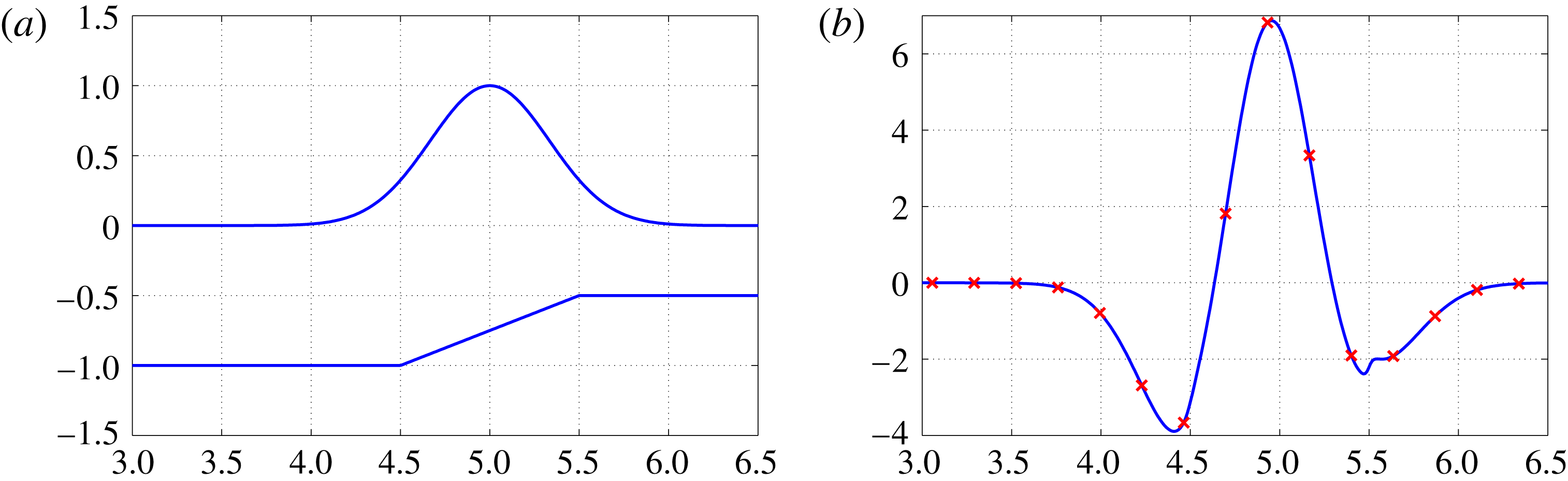
(a) Gaussian potential along the undisturbed free surface (
 $z=0$
) over a large-amplitude sloping bottom located at
 $(4.5\leqslant x\leqslant 5.5;-1\leqslant z\leqslant -0.5)$
. This slope is a detail of a bottom topography similar to that displayed in figure 3. (b) The respective Neumann data
 $\unicode[STIX]{x1D719}_{z}(x,0)$
computed through the DtN operator acting on the Gaussian potential (
 $\unicode[STIX]{x1D707}=0.05$
). The solid curve was obtained through (3.2) and (3.3). The red crosses were computed with the conformal mapping technique (3.27). For a better visualization, only a subset of the crosses are depicted. Both methods used
 $2^{10}$
points. All modes were used for the topographic component.

In order to compare the two methods, we start with the time-independent example as given by (3.24)–(3.26). As our Dirichlet data, we consider a Gaussian pulse located above the sloping bottom, as depicted in figure 1(a). This slope is a detail of a bottom topography similar to that displayed in figure 3. The bottom topography is not smooth. In figure 1(b) the solution with the present non-local method (solid line) is in very good agreement with that computed through the conformal mapping method (crosses).
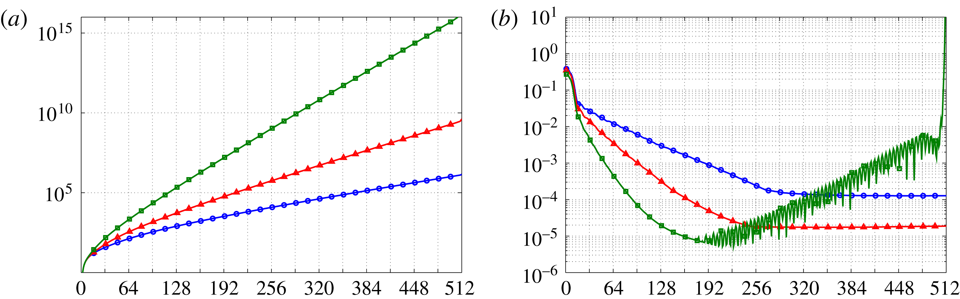
Figure 2 displays a resolution study for the Galerkin approximation, at different values of
 $\unicode[STIX]{x1D707}$
, as the number
 $n_{M}$
of active modes increases. Figure 2(a) has a log plot of the condition number of matrix
 $\unicode[STIX]{x1D63D}_{M}$
as a function of
 $n_{M}$
. Three wave regimes were considered:
 $\unicode[STIX]{x1D707}=0.05$
,
 $\unicode[STIX]{x1D707}=0.1$
and
 $\unicode[STIX]{x1D707}=0.2$
. The condition number grows exponentially with
 $n_{M}$
. Consider a grid with
 $2^{10}=1024$
nodes. For
 $\unicode[STIX]{x1D707}=0.05$
and
 $\unicode[STIX]{x1D707}=0.1$
, the condition number of
 $\unicode[STIX]{x1D63D}_{M}=B$
(considering all Fourier modes available) is, respectively,
 $1.32\times 10^{6}$
and
 $3.48\times 10^{9}$
. MATLAB computes using 16 digits of accuracy. Therefore, in the worst (
 $10^{9}$
) case, one still has of the order of seven digits of accuracy to rely on. Figure 2(b) displays a log plot for the relative error between the Galerkin approximation and the solution with the conformal mapping technique. Considering all Fourier modes available, the relative errors are
 $1.87\times 10^{-5}$
and
 $1.27\times 10^{-4}$
for
 $\unicode[STIX]{x1D707}=0.1$
and
 $\unicode[STIX]{x1D707}=0.05$
, respectively. We observe that the relative error saturates after a given
 $n_{M}$
. We also note that the shallower (
 $\unicode[STIX]{x1D707}=0.05$
) regime is approximately a decade worst than for
 $\unicode[STIX]{x1D707}=0.1$
. In the absence of an exact solution, we compare the present DtN method with the conformal mapping technique which has numerical difficulties with fine-scale variations within very elongated regions (Driscoll & Trefethen Reference Driscoll and Trefethen2002). Beyond a certain point the small relative error did not improve when allowing for higher frequencies. On the other hand, for the regime with
 $\unicode[STIX]{x1D707}=0.2$
, the relative error of the topographic part of the operator has numerical problems when using more than 160 active modes.
(a) Log plot of the condition number for matrix
 $\unicode[STIX]{x1D63D}_{M}$
as a function of
 $n_{M}$
, the number of active Fourier modes. We consider the simulation of figure 1 with different values of
 $\unicode[STIX]{x1D707}$
. The blue lines with circles correspond to
 $\unicode[STIX]{x1D707}=0.05$
, the red lines with triangles to
 $\unicode[STIX]{x1D707}=0.1$
and the green lines with squares to
 $\unicode[STIX]{x1D707}=0.2$
. (b) Log plot of the relative error between the Galerkin approximation and the conformal mapping solution, as a function of
 $n_{M}$
.

As mentioned in the introduction, Vasan & Deconinck (Reference Vasan and Deconinck2013) made a contribution in the context of time-dependent AFM simulations, in the presence of topography. Their goal was to recover the bottom profile from surface measurements. This task required an accurate time-dependent numerical modelling. Long, small-amplitude waves were used for the bottom reconstruction. To contrast with the present simulations, their dispersion parameter
 $\unicode[STIX]{x1D707}$
was set to
 $0.016$
in most of the simulations. Attention was paid to the number of Fourier modes needed to reconstruct the bottom accurately. The smooth obstacles considered were wavy bottoms and Gaussian mounds, among others. Their amplitude ranged up to
 $25\,\%$
of the total depth of the fluid. In most cases the typical number of Fourier modes was approximately 12 for the bottom and around 60 for the wave. As discussed in detail in Vasan & Deconinck (Reference Vasan and Deconinck2013), the use of a large number of Fourier modes can become an issue, in particular in the presence of topography and of moderate values of
 $\unicode[STIX]{x1D707}$
. Figure 2 confirms their statement but the Galerkin method shows that a larger number of Fourier modes can be used even in the presence of large-amplitude topographies.
4 Water wave simulations
We now present numerical results for the time evolution of surface water waves propagating over highly variable topographies. The time evolution has been performed with the fourth-order Runge–Kutta method.
We use the following initial data along the free surface
 $z=0$
:
 $$\begin{eqnarray}\displaystyle & \displaystyle \unicode[STIX]{x1D719}(x,0,0)=\text{e}^{-((x-x_{0})/\unicode[STIX]{x1D70E})^{2}} & \displaystyle\end{eqnarray}$$
is the initial velocity potential. We use
 $\unicode[STIX]{x1D70E}=1/6$
so that the pulse is approximately of unit width, centred at
 $x=x_{0}$
; the initial wave elevation is
 $$\begin{eqnarray}\displaystyle & \displaystyle \unicode[STIX]{x1D702}(x,0)=F^{-1}\left[\frac{k\,\text{tanh}(\unicode[STIX]{x1D707}k)}{\unicode[STIX]{x1D707}}F[\unicode[STIX]{x1D719}]\right]. & \displaystyle\end{eqnarray}$$
In the simulations we approximate the Fourier transform
 $F$
and its inverse
 $F^{-1}$
with the FFT.
In the three-dimensional simulations we have a plane wave with the above profile.
4.1 Two-dimensional results
We start with two-dimensional simulations, where results are known and we can further compare with the conformal mapping technique.
4.2 Waves over a submerged structure
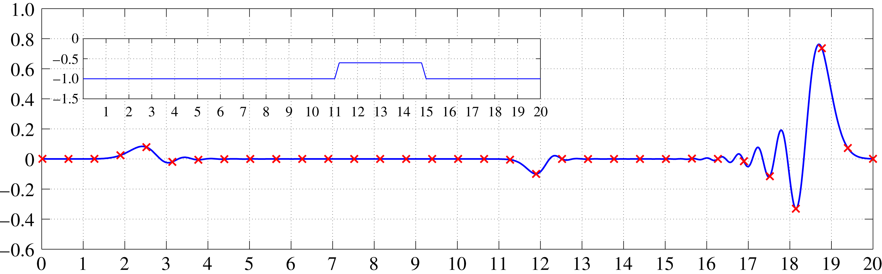
We again consider a non-smooth topography, now in the form of a large submerged trapezoidal structure. In the conformal mapping technique, the Jacobian is a smooth function along the free surface and therefore the corners of the submerged structure have been regularized. In the present method the topography comes into the formulation in its original form.
A Gaussian pulse of unit width for
 $\unicode[STIX]{x1D719}$
(similar to that of figure 1) propagates from the left (
 $x<10$
) towards the submerged structure located at
 $11<x<15$
(see inset of figure 3). The conformal mapping method follows the work presented in Artiles & Nachbin (Reference Artiles and Nachbin2004). A snapshot of the wave elevation at time
 $t=12$
is shown in figure 3. The agreement between the two methods is very good, regarding both the dispersive wave profile as well as the phase speed. We used
 $\unicode[STIX]{x1D707}=0.05$
, and dispersion, manifested through the oscillatory coda, is promptly observed. The solid line depicts the solution with the present method while the crosses depict results with the conformal mapping technique. Also the two reflected waves (due to climbing and descending from the structure) are accordingly captured by the methods. For both simulations we used
 $2^{10}$
points in physical space, and we considered all the Fourier modes available in our computational grid.
Wave profile observed after
 $12$
units of time. The solution with the present DtN method is displayed by a solid line and with crosses for the conformal mapping technique. For a better visualization, only a subset of the crosses are depicted. The wave regime corresponds to
 $\unicode[STIX]{x1D707}=0.05$
. The inset shows the topography at
 $11<x<15$
with an amplitude of 0.5, half the depth.

We should also mention that we found a maximum relative error of
 $6.275\times 10^{-4}$
, confirming the very good agreement between the two methods in this example.
4.3 Periodic topographies
In this section we study a wave moving from a region of constant depth towards a periodic patch of large-amplitude depth variations. This is a problem with known mathematical results and is a good test for our DtN formulation, in particular the calculation of its topographic coefficients with our Galerkin approach. We consider mean-zero periodic depth variations with an amplitude as high as half of the channel depth. The wave–topography interaction is considered in two different regimes. First the topographic variations are on the same scale as the wave field. Then we allow for large-amplitude, rapidly varying depth variations, a non-trivial test for the present DtN formulation. In this regime the bottom slope is large, while the wave feels the topography in an averaged form, as reported by Rosales & Papanicolaou (Reference Rosales and Papanicolaou1983).
From now on only our numerical solution will be presented.
4.3.1 Bragg resonance
In the context of water waves, Bragg resonance arises when the wavelength is twice as long as the topography’s period. The reflection is maximum in this regime. This is a known problem in water waves, and to provide a few references we mention the work of Mei (Reference Mei1985), regarding linear waves, and the more recent work of Choi & Milewski (Reference Choi and Milewski2003), regarding nonlinear waves. The setting for our simulations differs from the theoretical work of Mei (Reference Mei1985) and Choi & Milewski (Reference Choi and Milewski2003). The topographies considered in the theoretical investigations had small amplitudes of order of
 $O(\unicode[STIX]{x1D707}^{2})$
. In the present simulations the channel’s depth oscillates from
 $0.5$
to
 $1.5$
.
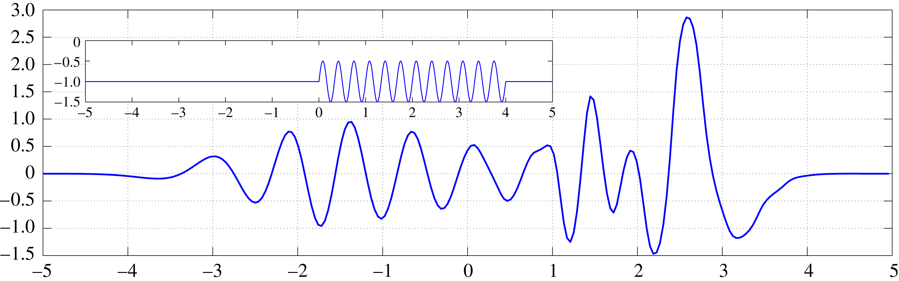
Evolution of the wave elevation after
 $4.5$
units of time. Note the nearly monochromatic structure of the reflected wave. The wave regime corresponds to
 $\unicode[STIX]{x1D707}=0.1$
. The inset shows the underwater sinusoidal topography. The numerical method used
 $2^{10}$
Fourier modes and the Galerkin method used
 $M=250$
(which corresponds to
 $397$
active Fourier modes out of
 $512$
) for the topographic component of the DtN operator.

In figure 4 we present a snapshot of the solution at time
 $t=4.5$
. A pulse propagates to the right, from the constant-depth region located at
 $x<0$
(see figure 4). As the wave propagates over the periodic patch, a (nearly) monochromatic reflected wave is observed (moving to the left) with a wavelength twice as long as the topography’s period. The observed reflected wavelength is
 $0.667$
(for
 $-2<x<0$
), where the sinusoidal topography has period
 $0.333$
.
4.3.2 Homogenization with a rapidly varying topography
Now we investigate rapidly varying periodic topographies. This is an important test to see if our DtN formulation accurately captures fine features of the topography. The topography has large slopes and we want to observe numerically the impact of our Galerkin approximation in handling the topographic component of the DtN operator.
Through a multi-scale analysis, Rosales & Papanicolaou (Reference Rosales and Papanicolaou1983) showed that a long wave feels the fine features of the topography in an averaged form. Namely a homogenization effect takes place to leading order. The wave behaves as if propagating over an ‘effectively flat’ region: no reflection is observed and the wave speed is smaller than the (dimensionless) unit speed. The periodic topography has mean zero but the wave behaves as if there was an effective depth smaller than 1. This was found by Rosales & Papanicolaou (Reference Rosales and Papanicolaou1983) in the weakly nonlinear, weakly dispersive case. The same result holds in the linear case, as reported in Nachbin (Reference Nachbin1993). The non-local formulation has been used in theoretical investigations of this phenomenon. Craig et al. (Reference Craig, Guyenne, Nicholls and Sulem2005) derived an asymptotically valid KdV equation from the non-local equations. Their KdV equation also has a smaller effective speed of propagation. Our simulations consider a large-amplitude, rapidly varying topography. As before, our topography varies from
 $0.5$
to
 $1.5$
and the sinusoidal bottom oscillates
 $12$
times per (unit) pulse width.
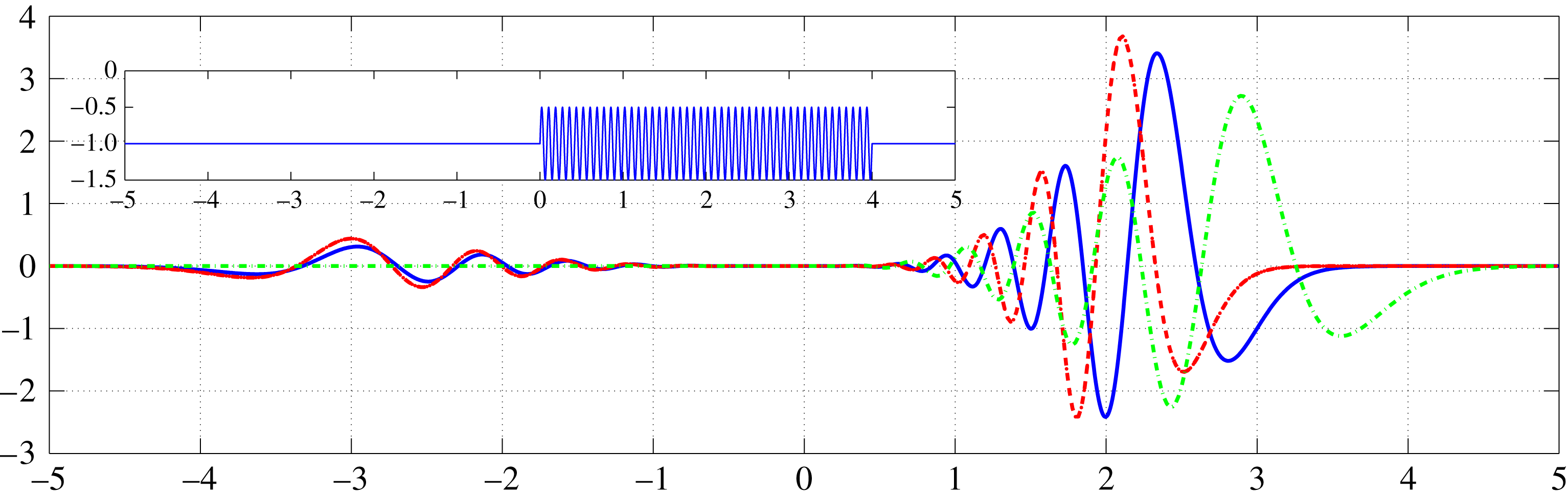
Homogenized wave field (blue solid line), simulation without topography (red dashed-dotted line) and simulation over the envelope of the bottom (green dashed line). All the simulations correspond to the regime
 $\unicode[STIX]{x1D707}=0.1$
. The numerical method used
 $2^{11}$
Fourier modes and the Galerkin method used
 $M=250$
(which corresponds to
 $397$
active Fourier modes out of
 $1024$
) for the topographic component of the DtN operator.

In figure 5 we superimpose three simulations: (i) a flat bottom case; (ii) a large-amplitude, mean-zero, rapidly varying periodic topography; and (iii) a step obtained as the envelope of the rapidly varying topography. The dispersion parameter is taken as
 $\unicode[STIX]{x1D707}=0.1$
. We should recall that the Galerkin parameter
 $M$
depends on
 $\unicode[STIX]{x1D707}$
. The shallow-water regime is easier to solve than a dispersive regime. The tests reported below were also done for a (nearly) travelling pulse in a very shallow channel, but we only report the more demanding dispersive case.
The green dashed line corresponds to the flat bottom case. No reflected wave is observed. At the wavefront we note the dispersive oscillatory tail. We focus on the speed at the wavefront, which in this case is
 $0.94$
due to the initial wave profile and dispersion. The red dashed-dotted line corresponds to the envelope of the bottom topography, namely a step. The wavefront appears behind the flat bottom case because over the step the speed of propagation is smaller, approximately
 $0.68$
. Finally, the blue solid line is the solution in the presence of the rapidly varying topography. The effective speed is smaller than the flat bottom case but larger than the step. This is our numerically homogenized wave field. No reflection is produced over the rapidly varying periodic topography. The bottom’s fine features were captured accordingly along the free surface through the DtN operator. The solution is free from numerical noise, indicating that the Galerkin approximation for the topographic coefficients of the non-local operator performed well. The numerically observed (effective) wave speed is
 $0.82$
. In the shallow-water case we clearly see a (nearly) travelling wave over the topography, with no reflected wave observed. The only reflected signal comes from the transition from flat to periodic.
4.4 The three-dimensional DtN operator: refraction by a submerged mound
In this section we investigate the refraction of two-dimensional surface waves due to bathymetric variations. We explore the changes in propagation direction as the wave passes over a circular submerged mound. We will report on a special mound, known as the Luneburg lens, where the front of an incoming plane wave bends in a particular fashion.
4.4.1 The Luneburg lens
We consider a particular submerged mound which, as we shall see, plays a role analogous to that of the Luneburg lens in optics. The mound focuses the wave energy at a determined point in space. Our goal is to show that the DtN operator, in our two-dimensional surface model, accurately captures the complex refraction pattern that arises due to the non-trivial change in depth.
The underwater mound is given by
 $$\begin{eqnarray}\displaystyle & \displaystyle H(r)=\left\{\begin{array}{@{}l@{}}{\displaystyle \frac{\unicode[STIX]{x1D6FC}^{2}}{\unicode[STIX]{x1D6FC}^{2}+1-(r/r_{0})^{2}}}-1,\quad \text{if}~r<r_{0},\quad \\ 0,\quad \text{if}~r\geqslant r_{0}.\quad \end{array}\right. & \displaystyle\end{eqnarray}$$
We consider
 $\unicode[STIX]{x1D6FC}=0.8$
,
 $r=\sqrt{(x-8)^{2}+(y-10)^{2}}$
and
 $r_{0}=4$
. The water depth above the centre of the mound is approximately
 $0.60$
. The numerical method used
 $2^{9}$
Fourier modes in each direction and the Galerkin method used
 $M=37.69$
for the topographic component of the DtN operator (which corresponds to
 $120$
active Fourier modes). The use of a smaller
 $M$
is due to memory restrictions. For a two-dimensional surface and
 $M=37.69$
we have
 $240^{2}$
Fourier modes representing functions in our respective subspace for the topographic component of DtN. In order to find the contribution for each of these Fourier modes, we need to build and invert a
 $240^{2}$
by
 $240^{2}$
matrix.
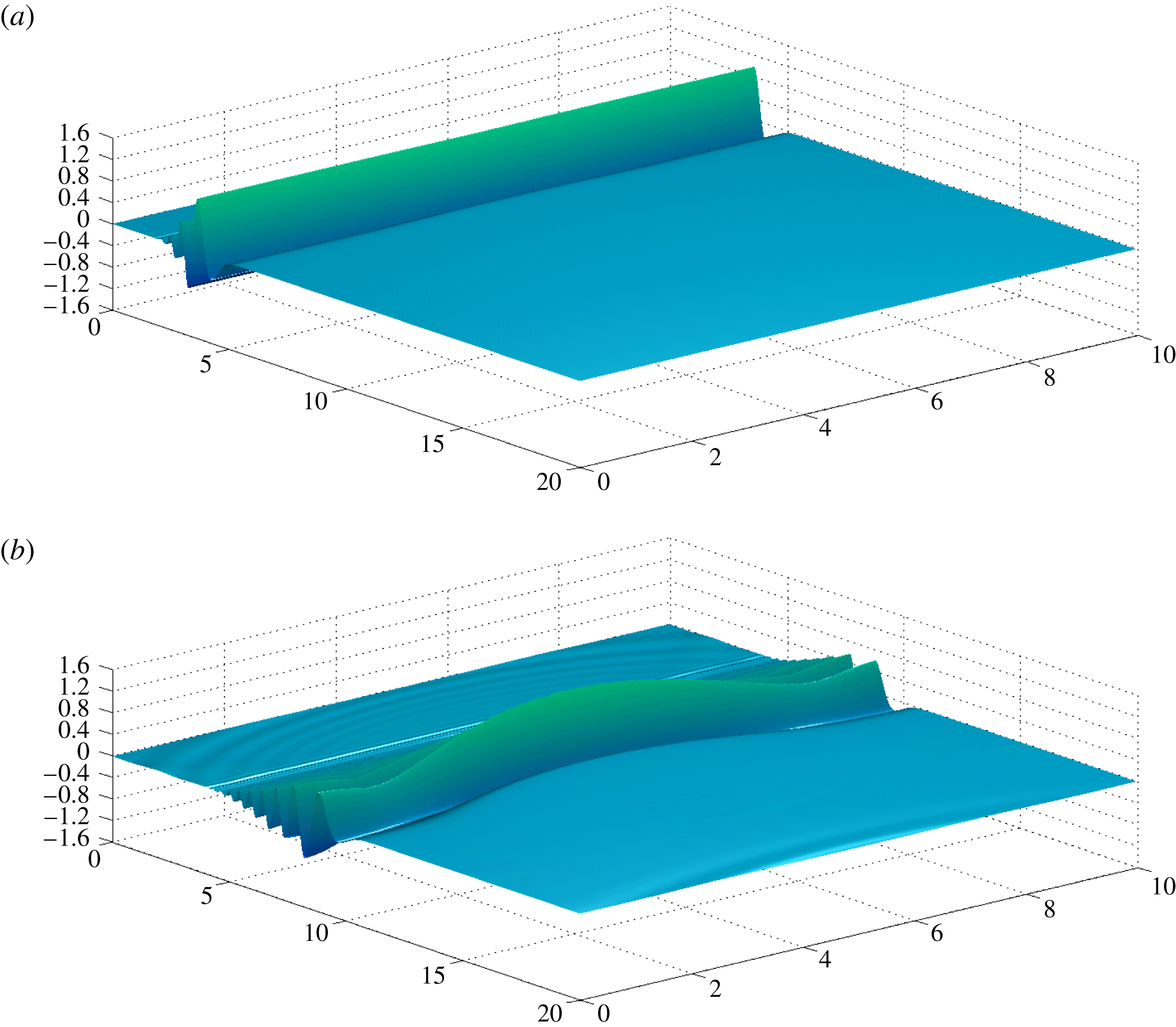
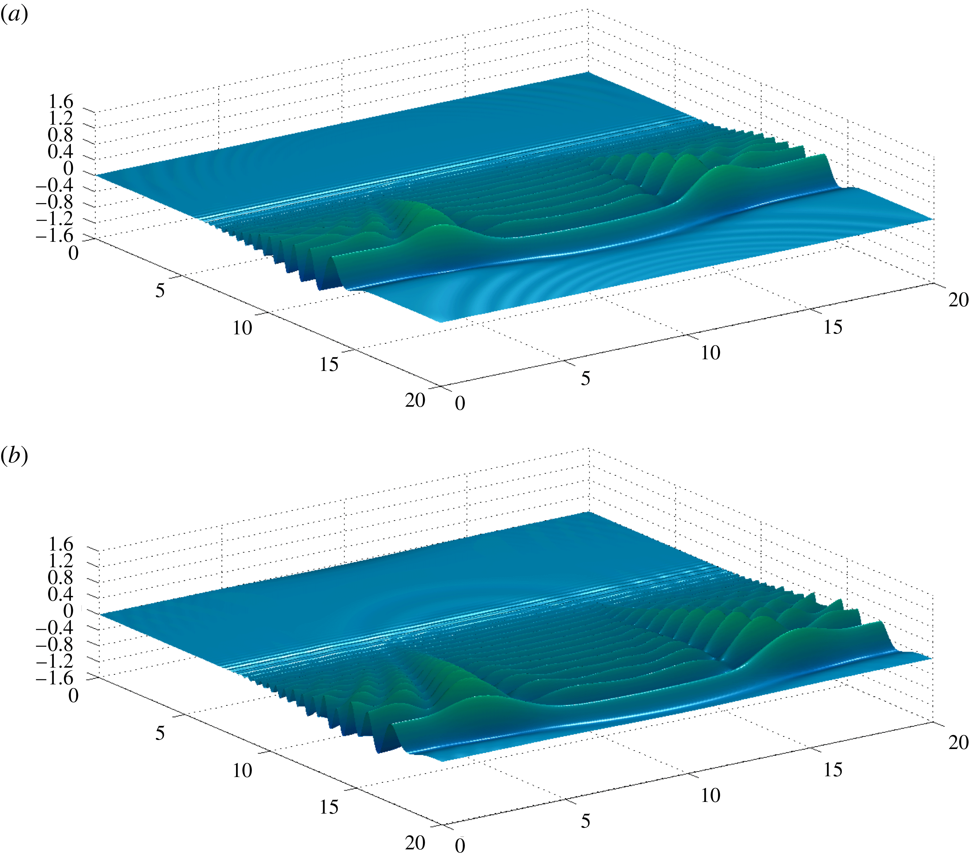
Four snapshots of the solution are presented in figures 6 and 7. In figure 6(a), corresponding to time
 $t=3.1$
, we see the incoming plane wave (from the left) already displaying some dispersive effect. We have used
 $\unicode[STIX]{x1D707}=0.1$
. A short oscillatory tail is apparent behind the wavefront. The topography is in the middle of the computational domain and no change of direction of propagation is observed.
Snapshots at times (a)
 $t=3.1$
and (b)
 $t=8.6$
. The incoming surface elevation is propagating towards the Luneburg lens (
 $\unicode[STIX]{x1D6FC}=0.8$
) in the
 $\unicode[STIX]{x1D707}=0.1$
regime. An animation for the corresponding velocity potential can be found in the supplementary material of this article at https://doi.org/10.1017/jfm.2018.241.

In figure 6(b), at time
 $t=8.6$
, we see a strong deformation along the wavefront due to its interaction with the submerged mound. The depth in the middle is decreasing and therefore the speed at the central part of wavefront is smaller.
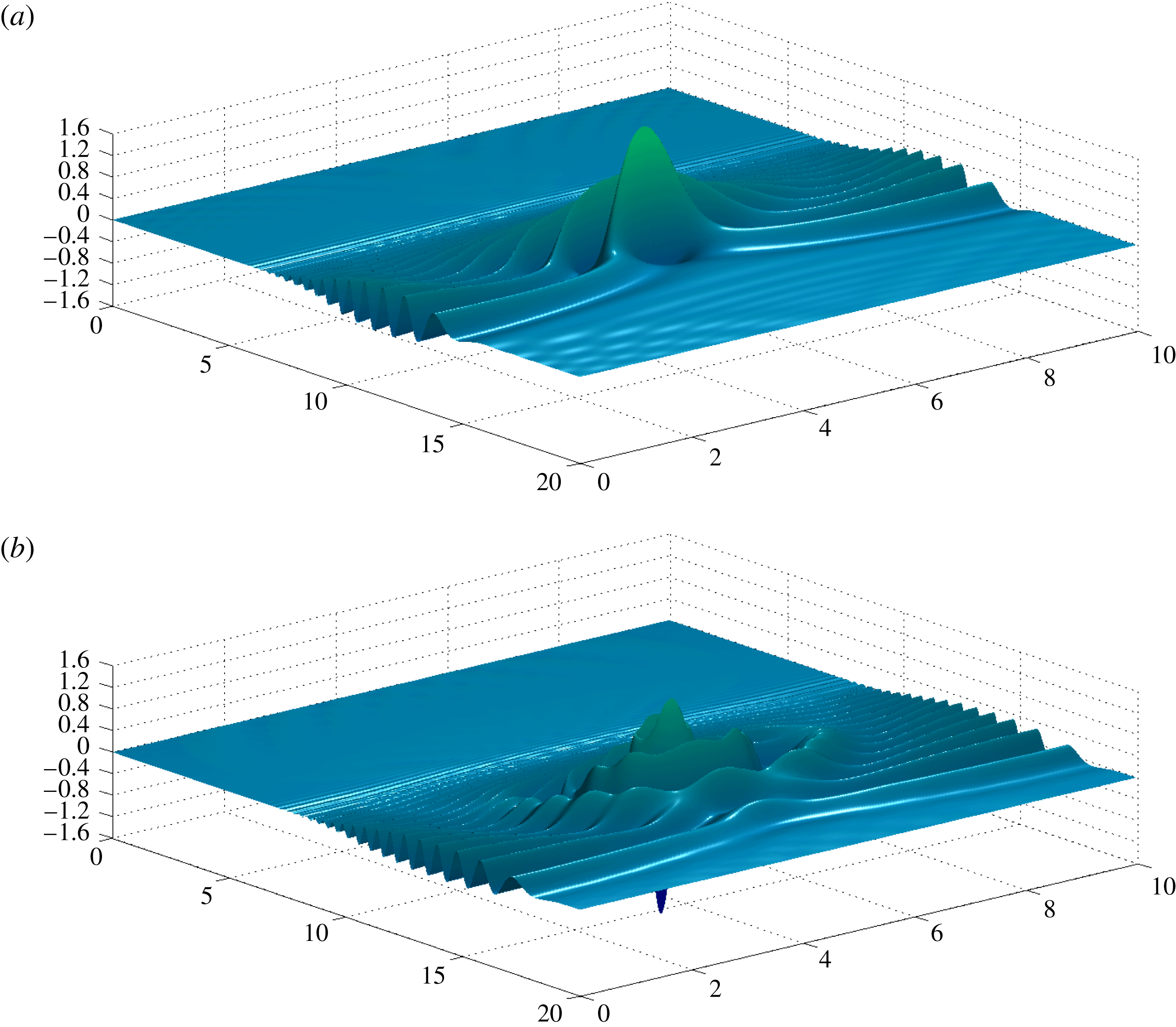
Snapshots at times (a)
 $t=13.6$
and (b)
 $t=17$
. The surface elevation is propagating over the Luneburg lens (
 $\unicode[STIX]{x1D6FC}=0.8$
) in the
 $\unicode[STIX]{x1D707}=0.1$
regime. The focusing due to refraction is clearly observed.

In figure 7(a) we have the solution at time
 $t=13.6$
. We observe the effect of the Luneburg lens: it focuses the wave energy at a point behind the mound. At this time the largest wave amplitude is observed, exactly at the focusing point, as will be confirmed below. The wave amplitude at the focusing point is approximately twice as high as that of the initial incoming wave. As the high-amplitude peak moves down due to gravity, smaller waves (of the dispersive tail) will focus behind it, giving rise to a circular pattern that eventually dominates the wave field, at time
 $t=17$
(figure 7
b). We tested with other shapes of the submerged mound (such as a Gaussian profiles) and of course the focusing effect does not take place.
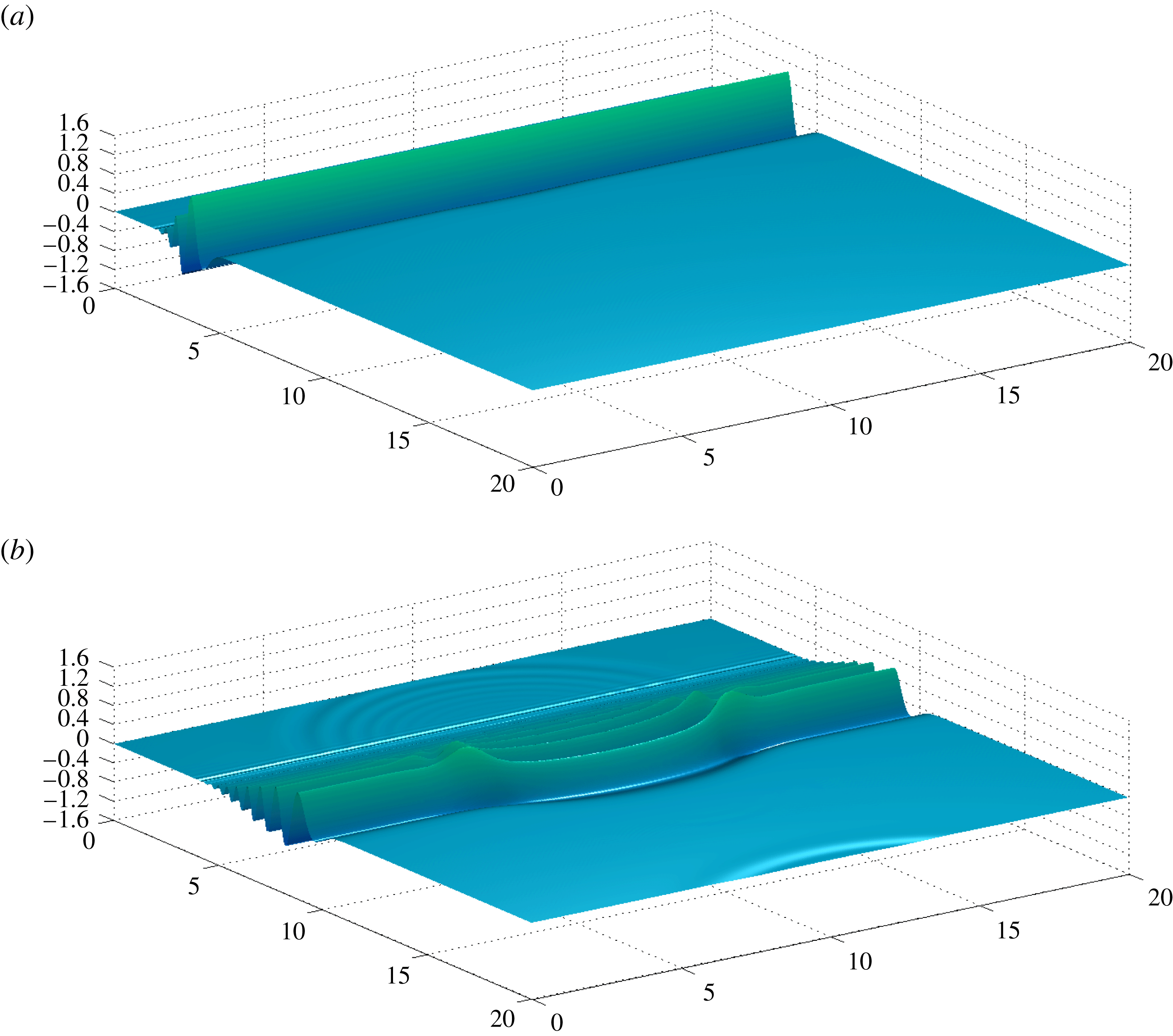
In particular, if the submerged Luneburg mound becomes concave, namely a circular cavity, the wavefront bending is in the other direction. The water becomes deeper and the wave propagates faster over the cavity. The submerged cavity is given by
 $-H$
as in (4.3). Snapshots of the corresponding numerical solution are given in figures 8 and 9. At time
 $t=3.1$
we have the usual incoming plane wave as shown in figure 6(a). At time
 $t=8.6$
we start to observe the refraction pattern, now with the wavefront moving forward at its central part.
Snapshots at times (a)
 $t=3.1$
and (b)
 $t=8.6$
. The incoming surface elevation is propagating towards a concave cavity (with the Luneburg lens profile;
 $\unicode[STIX]{x1D6FC}=0.8$
) in the
 $\unicode[STIX]{x1D707}=0.1$
regime.

Snapshots at times (a)
 $t=13.6$
and (b)
 $t=17$
. The surface elevation is propagating over a concave cavity (with the Luneburg lens profile;
 $\unicode[STIX]{x1D6FC}=0.8$
) in the
 $\unicode[STIX]{x1D707}=0.1$
regime.

We used the spmd function, from MATLAB’s Parallel Computing Toolbox, to distribute the matrices
 $\unicode[STIX]{x1D63C}$
and
 $\unicode[STIX]{x1D63D}_{M}$
among
 $16$
nodes on a computer cluster. The matrix
 $\unicode[STIX]{x1D63D}_{M}^{-1}\unicode[STIX]{x1D63C}$
is computed only once and used with the classical Runge–Kutta method for the time evolution. In the Luneburg lens simulation, the condition number of the
 $240^{2}\times 240^{2}$
 $\unicode[STIX]{x1D63D}_{M}$
matrix is
 $1.674\times 10^{3}$
. Having in mind that MATLAB uses 16 digits of accuracy, ill-conditioning is not effective at all in this problem. Recall also that we have 120 active Fourier modes (47 %) of a total of 256. The time spent on the computation of the
 $\unicode[STIX]{x1D63D}_{M}^{-1}\unicode[STIX]{x1D63C}$
operator represented approximately
 $55\,\%$
of the total simulation.
Both simulations show that our numerical method, based on the construction of a three-dimensional DtN operator, accurately captured interesting refraction patterns due to lens-like bottom topographies. In the next subsection an approximate ray theory, for the dispersive equations, confirms the accuracy in the Luneburg lens case.
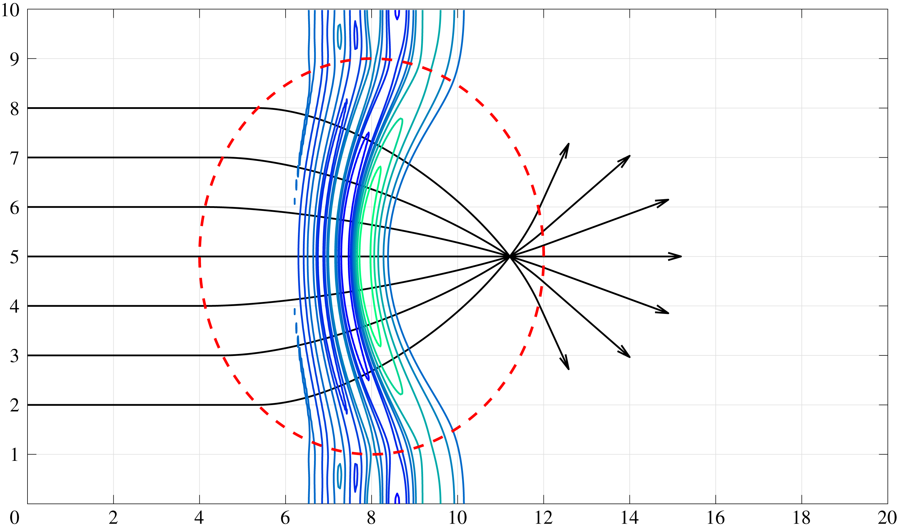
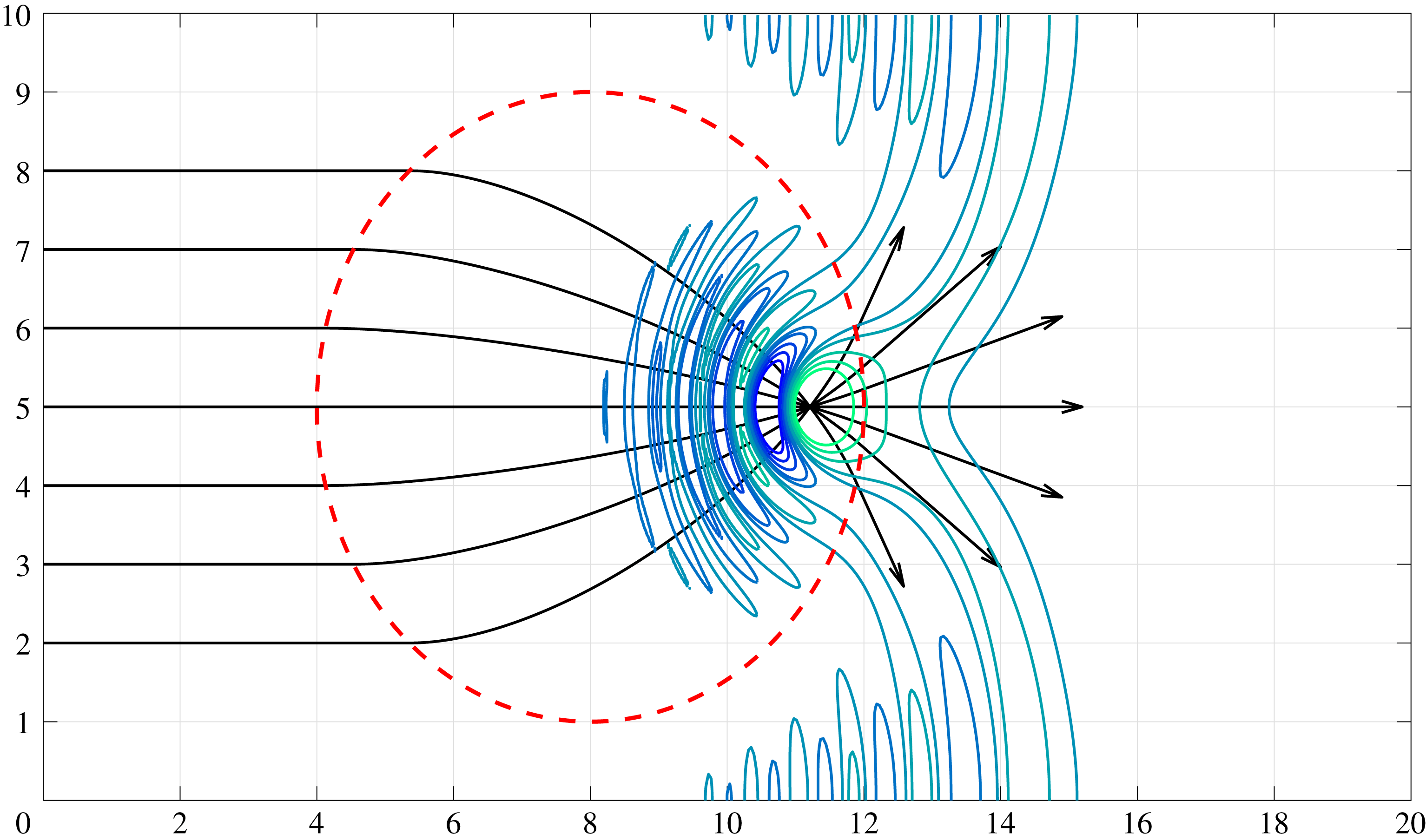
4.4.2 Ray theory
We aim to compare the refraction pattern of the numerical wave field against predictions from the theory of refraction for monochromatic waves. This is a classical subject in the geometrical optics theory for water waves. A detailed treatment can be found in the literature (Dingemans Reference Dingemans1997; Johnson Reference Johnson1997; Whitham Reference Whitham1999). Our model is reduced to three equations that provide a first-order approximation for the refraction pattern of a nearly monochromatic wavetrain. The monochromatic approximation is suitable for our purposes since we have a linear wave model. We consider the long-wave regime, where dispersion is weak (
 $\unicode[STIX]{x1D707}$
is small).
The approximation begins with the following ansatz for the velocity potential:
 $$\begin{eqnarray}\displaystyle & \displaystyle \unicode[STIX]{x1D719}(x,y,t)=a(x,y)\text{e}^{\text{i}(\unicode[STIX]{x1D703}(x,y)-\unicode[STIX]{x1D714}t)}. & \displaystyle\end{eqnarray}$$
The velocity potential is taken as an oscillatory wavetrain that is modulated with an amplitude function
 $a(x,y)$
and a phase function
 $\unicode[STIX]{x1D703}(x,y)$
. Both functions
 $a$
and
 $\unicode[STIX]{x1D703}$
are assumed to vary on a scale faster than the depth variations of the Luneburg lens. The phase
 $\unicode[STIX]{x1D703}$
is determined by the eikonal equation
 $$\begin{eqnarray}\unicode[STIX]{x1D703}_{x}^{2}+\unicode[STIX]{x1D703}_{y}^{2}=\unicode[STIX]{x1D70E}^{2},\end{eqnarray}$$
where
 $$\begin{eqnarray}\unicode[STIX]{x1D714}^{2}={\displaystyle \frac{\unicode[STIX]{x1D70E}}{\unicode[STIX]{x1D707}}}\tanh (\unicode[STIX]{x1D707}(1+H(\boldsymbol{x}))\unicode[STIX]{x1D70E}).\end{eqnarray}$$
We have an
 $\boldsymbol{x}$
-dependent dispersion relation that determines the variable wavenumber
 $\unicode[STIX]{x1D70E}(\boldsymbol{x})$
. It plays the role of a variable index of refraction in the eikonal equation for
 $\unicode[STIX]{x1D703}$
. We use the method of characteristics to solve equation (4.5). In this context it is customary to call the characteristic curves
 $(x,y)$
‘rays’. It is also known that the wavefronts (level curves in
 $\unicode[STIX]{x1D703}$
) are orthogonal to the rays/characteristics (Zauderer Reference Zauderer1989).
The Cauchy problem for the eikonal equation consists in determining the phase function
 $\unicode[STIX]{x1D703}$
from an ‘initial’ constant data
 $\unicode[STIX]{x1D703}_{0}$
along the
 $y$
axis. First we need to determine the function
 $\unicode[STIX]{x1D70E}$
from the dispersion relation (4.6). Note that outside the circle
 $r=r_{0}$
,
 $H$
vanishes, and therefore, in that region, the solution to (4.6) is given by a constant
 $\unicode[STIX]{x1D70E}_{0}$
. Inside the circle we solve the dispersion equation numerically by means of Newton’s method.
Once the function
 $\unicode[STIX]{x1D70E}$
and its derivatives are determined, we are ready to solve the characteristic equations given by
 $$\begin{eqnarray}\displaystyle \left.\begin{array}{@{}l@{}}{\displaystyle \frac{\text{d}x}{\text{d}\unicode[STIX]{x1D70F}}}=2p,\quad \text{with}~x(0,s)=0,\\[9.0pt] {\displaystyle \frac{\text{d}y}{\text{d}\unicode[STIX]{x1D70F}}}=2q,\quad \text{with}~y(0,s)=s,\\[9.0pt] {\displaystyle \frac{\text{d}p}{\text{d}\unicode[STIX]{x1D70F}}}={\displaystyle \frac{\unicode[STIX]{x2202}\unicode[STIX]{x1D70E}^{2}}{\unicode[STIX]{x2202}x}},\quad \text{with}~p(0,s)=p_{0}(s),\\[9.0pt] {\displaystyle \frac{\text{d}q}{\text{d}\unicode[STIX]{x1D70F}}}={\displaystyle \frac{\unicode[STIX]{x2202}\unicode[STIX]{x1D70E}^{2}}{\unicode[STIX]{x2202}y}},\quad \text{with}~q(0,s)=q_{0}(s),\\[9.0pt] {\displaystyle \frac{\text{d}\unicode[STIX]{x1D703}}{\text{d}\unicode[STIX]{x1D70F}}}=2\unicode[STIX]{x1D70E}^{2},\quad \text{with}~z(0,s)=\unicode[STIX]{x1D703}_{0}.\end{array}\right\} & & \displaystyle\end{eqnarray}$$
In these equations we define
 $(p,q)=\unicode[STIX]{x1D735}\unicode[STIX]{x1D703}$
along the rays, which are parametrized by
 $\unicode[STIX]{x1D70F}$
. The complete set of initial data must satisfy the following conditions, known as the strip conditions (Zauderer Reference Zauderer1989):
 $$\begin{eqnarray}\displaystyle \left.\begin{array}{@{}l@{}}p_{0}^{2}(s)=\unicode[STIX]{x1D70E}_{0}^{2},\\ q_{0}(s)=0.\end{array}\right\} & & \displaystyle\end{eqnarray}$$
The characteristic system (4.7) is solved using the fourth-order Runge–Kutta method. In figures 10 and 11 the black solid lines correspond to the rays
 $(x(\unicode[STIX]{x1D70F},s),y(\unicode[STIX]{x1D70F},s))$
. Note how the rays bend and focus into one point inside the lens, represented by the red circle. This focusing property distinguishes the Luneburg lens from other types of submerged mounds. In figure 10 we also plot some level curves of our numerical wave solution, computed with the non-local DtN method. Note that before the caustics, where the method of characteristics breaks down, the rays and wavefronts are nearly orthogonal, as expected. Later in time, in figure 11, we see the focusing of the wave field at exactly the point where the rays meet. The point where the rays focus through the method of characteristics is
 $(11.21,5)$
, whereas the wave field, from our non-local method, attains its maximum at
 $(11.28,5)$
.
Evolution of a Gaussian velocity potential over a Luneburg lens with parameters
 $\unicode[STIX]{x1D6FC}=0.8$
at time
 $8.6$
. The black lines correspond to the rays. Note that the wavefronts, the level lines of the velocity potential, follow the rays. The dispersion parameter is
 $\unicode[STIX]{x1D707}=0.1$
.

Evolution of a Gaussian velocity potential over a Luneburg lens with parameters
 $\unicode[STIX]{x1D6FC}=0.8$
, in the
 $\unicode[STIX]{x1D707}=0.1$
regime, at time
 $13.6$
. The black lines correspond to the rays. Note that the wave field focuses on top of the point where the rays meet.

Our three-dimensional simulations captured very well theoretical predictions. In the examples considered, the topography had a non-trivial amplitude and our method captured remarkably well the predicted dynamical features.
5 Conclusions
We have constructed a Dirichlet-to-Neumann (DtN) operator for a three-dimensional (surface) water wave problem in the presence of highly variable, non-smooth, topographies. The DtN operator captures the vertical structure of the flow and allows the three-dimensional problem to be reduced to a two-dimensional surface. The few existing articles on the DtN formulation in the presence of topography consider mostly small-amplitude, smooth bottom variations. Owing to memory and numerical stability issues, the three-dimensional problem had not been explored numerically. By using a Galerkin projection onto the relevant modes that indeed interact with the topography, we have been able to exhibit several accurate simulations in the presence of non-trivial bottom profiles.
In particular we considered a circular submerged mound that plays the role of a Luneburg lens, known in optics. The mound bends the wavefront, through refraction, focusing the energy behind the lens. Our three-dimensional DtN formulation captured quite accurately the focusing/refraction of the incident plane wave. Using an approximate ray theory for the dispersive (long-)wave formulation, we showed that the focusing point is found with excellent accuracy.
Acknowledgements
D.A. gratefully acknowledges support by the PNPD/CAPES programme. The work of A.N. was supported in part by CNPq under (PQ-1B) 301949/2012-2 and FAPERJ Cientistas do Nosso Estado project no. E-26/201.164/2014. The authors acknowledge fruitful discussions with P. Milewski. The authors thank two referees for their valuable comments.
Supplementary movie
Supplementary movie is available at https://doi.org/10.1017/jfm.2018.241.