The BIMNL Model

The BIMNL estimator combines two latent equations: a logit equation, which we denote as the “first-stage” estimator and an MNL equation hereafter referred to as the “outcome-stage” estimator. To motivate this model, consider a dependent variable Y _i with i∈{1, 2, … , N} respondents (e.g., individuals). Suppose further that Y _i is observable and assumes the discrete unordered values of 0,1, … , J, with value Y _i =0 representing a baseline “abstain” category. Next, let s _i denote a binary variable that indicates a split between regime 0 (s _i =0) and regime 1 (s _i =1), wherein s _i =0 denotes “inflated abstainers” that will always fall within the residual baseline category of Y _i and s _i =1 denotes “noninflated abstainers” who may choose to abstain in a given instance, but who may also potentially select an option in 1, … , J. In the context of a vote choice survey data set, the abstain responses in regime 0 (s _i =0) would include routine nonvoters who never choose to vote, whereas responses in regime 1 (s _i =1) include occasional nonvoters whose probability of transitioning to a candidate vote choice outcome is not zero. Note that s _i is related to the latent-dependent variable $s_{i}^{{\rm {\asterisk}}} ,$ such that s _i =1 for $s_{i}^{{\rm {\asterisk}}} \gt \,0$ and s _i =0 for $s_{i}^{{\rm {\asterisk}}} \leq 0$ . The latent variable $s_{i}^{{\rm {\asterisk}}} $ represents the propensity for entering regime 1 and is given by the following linear additive specification, which we refer to as the latent inflation equation:

(1) $$s_{i}^{{\rm {\asterisk}}} ={\bf z\prime}\!_{i} {\bf \gamma }{\plus}u_{i} .$$

The inflation equation in 1, once re-stated via a binary (logistic) response model for our dichotomous regime indicator s _i , constitutes the first stage of the BIMNL model. In equation (1), ${\bf z\prime}\!_{i} $ is the vector of covariates, γ the vector of coefficients and u _i is a standard-logistic distributed error term. Hence, the probability of i being in regime 1 is $${\rm Pr}(s_{i} =1\!\mid\!{\bf z}_{i} )={\rm Pr}(s_{i}^{{\rm {\asterisk}}}\, \gt \,0\!\mid\!{\bf z}_{i} )={\rm \Lambda }({\bf z\prime}\!_{i} { \bigamma })$$ , and the probability that i is in regime 0 is ${\rm Pr}(s_{i} =0\!\mid\!{\bf z}_{i} )={\rm Pr}(s_{i}^{{\rm {\asterisk}}} \leq 0\!\mid\!{\bf z}_{i} )=1{\minus}{\rm \Lambda }({\bf z\prime}\!_{i} {\bf \gamma }),$ where $\Lambda ( \cdot )$ is the logistic cumulative distribution function (c.d.f.).

If s _i =1, then the observations in regime 1 are given by the discrete unordered variable $\tilde{Y}_{i} ,$ which can take on any of J unordered values, and where ${\rm Pr}(\tilde{Y}_{i} =j)=P_{{ij}} $ . In noting that by definition, $\mathop{\sum}\nolimits_{j\,=\,0}^J {P_{{ij}} =1} $ , we then allow the probability of $\tilde{Y}_{i} =j\in J$ to vary as a function of some k independent variable(s) x _i , indexed by a K×1 vector of parameters specific to outcome β _j by restricting the probabilities to be positive and sum to one as so:

(2) $${\rm Pr}(\tilde{Y}_{i} =j)\,\equiv\,P_{{ij}} ={{e^{{{\bf x'}_{i} \beta _{j} }} } \over {\sum_{j\,=\,0}^J e^{{{\bf x'}_{i} \beta _{j} }} }}.$$

Hence, observation i’s probability associated with category j is expressed as a fraction of the sum of all of observation i’s probabilities across the various categories J. This ensures that Pr(Y _i =j)∈(0,1) and that $$\mathop{\sum}\nolimits_{j\,=\,0}^J {{\rm Pr}(\tilde{Y}_{i} =j)=1} $$ . Under the assumption that the corresponding error term (ε _i ) for Equation 2 is independently and identically distributed (i.i.d) according to a Type I Extreme Value distribution, Equation 2 denotes the primary statement of probability for the MNL model. However, this model is also unidentified: knowing the (J−1)×k values of β ₀, β ₁, … , β _J−1, also provides one with the probability of choosing the remaining alternative. To identify the above MNL probabilities for estimation, we follow common practice and set the parameters for the first of the J alternatives to 0, that is, β ₀, which we refer to hereafter as the baseline category. Doing so allows us to restate the probabilities for the baseline category $({\rm Pr}(\tilde{Y}_{i} =0))$ and the other J−1 categories separately as:

(3) $${\rm Pr}(\tilde{Y}_{i} )=\left\{ {\matrix{ {\quad \quad \,{\rm Pr}(\tilde{Y}_{i} =0\!\mid\!{\bf x}_{i} ,s_{i} =1)={1 \over {1{\plus}\sum_{j=1}^J e^{{{\bf x'}_{i} \beta _{j} }} }}} \hfill \cr {{\rm Pr}(\tilde{Y}_{i} =j\!\mid\!{\bf x}_{i} ,s_{i} =1)={{e^{{{\bf x'}_{i} \beta _{j} }} } \over {1{\plus}\sum_{j=1}^J e^{{{\bf x'}_{i} \beta _{j} }} }}{\rm }(j=1,\:\,\ldots\,\:,J)} \hfill \cr {} \hfill \cr } } \right\},$$

where β _j =β _j −β ₀ are now “rescaled” parameters in that they express the influence of the various x’s on ${\rm Pr}(\tilde{Y}_{i} =j)$ relative to ${\rm Pr}(\tilde{Y}_{i} =0)$ .

Note that neither $\tilde{Y}_{i} $ nor s _i are observable in terms of the observed baseline outcomes. However, they are observed by the criterion $Y_{i} =\tilde{Y}_{i} {\times}s_{i} $ . The aforementioned expression thus implies that the (baseline) outcome Y _i =0 can occur when s _i =0 or when s _i =1 and $\tilde{Y}_{i} =0$ . It also indicates that we can observe Y _i =1, … ,J only when s _i =1 and $$\tilde{Y}_{i} =1,\:\:...\:,J$$ . Accordingly, the BIMNL distribution arises as a mixture of a degenerate distribution in the baseline category and the assumed distribution of the variable $\tilde{Y}_{i} $ as follows:

(4) $${\rm Pr}(Y_{i} )=\left\{ {\matrix{ {{\rm Pr}(s_{i} =0\!\mid\!{\bf z}_{i} ){\plus}{\rm Pr}(s_{i} =1\!\mid\!{\bf z}_{i} )\,{\rm Pr}(\tilde{Y}_{i} =0\!\mid\!{\bf x}_{i} ,s_{i} =1)\,{\rm for}\,j=0} \hfill \cr {{\rm Pr}(s_{i} =1\!\mid\!{\bf z}_{i} )\,{\rm Pr}(\tilde{y}_{i} =j\!\mid\!{\bf x}_{i} ,s_{i} =1)\,{\rm for}\,\,j=1,2,\:\:\,\ldots\!\:,\,J} \hfill \cr } } \right\}.$$

Under the assumption that u _i and ε _i identically and independently follow standard Type I Extreme Value distributions, the BIMNL model can thus be defined as:

(5) $${\rm Pr}(Y_{i} )=\left\{ {\matrix{ {{\rm Pr}(Y_{i} =0\!\mid\!{\bf x}_{i} ,{\bf z}_{i} )=[1{\minus}{\rm \Lambda }({\bf z\prime}\!_{i} \gamma )]{\plus}\left( {{{{\rm \Lambda }({\bf z\prime}\!_{i} \gamma )} \over {1{\plus}\sum_{j=1}^J e^{{{\bf x\prime}\!_{i} \beta _{j} }} }}} \right)} \hfill \cr {{\rm Pr}(Y_{i} =j\!\mid\!{\bf x}_{i} ,{\bf z}_{i} )=\left( {{{{\rm \Lambda }({\bf z\prime}\!_{i} \gamma )e^{{{\bf x\prime}\!_{i} \beta _{j} }} } \over {1{\plus}\sum_{j=1}^J e^{{{\bf x\prime}\!_{i} \beta _{j} }} }}} \right){\rm }(j=1,\:\:\,\ldots\!\:,J)} \hfill \cr {} \hfill \cr } } \right\},$$

where, as above, $\Lambda ( \cdot )$ is the logistic c.d.f. The expression in 5 thus provides the full probabilities of the BIMNL model. Herein, the probability of observing a baseline-choice observation within the baseline equation of the BIMNL model is modeled conditional upon the probability of an observation being assigned a baseline value in the multinomial data generating process (d.g.p.) plus the probability of it being in regime 0 from the inflation equation. As a result, when the unordered dependent variable is baseline inflated and thus has two types of baseline observations, the BIMNL model allows researchers to obtain more accurate estimates relative to a standard MNL model, which is to say that the BIMNL estimates are both less biased and have greater coverage probabilities. We demonstrate these points in the Monte Carlo simulations reported in our supplemental appendix. The remaining probabilities in 5 then correspond to the conditional probabilities of an observation choosing a polytomous choice value other than the baseline value, conditional on an observation being in the MNL state of the world.

Having described the conditional probabilities for the BIMNL model above, we can now define the likelihood and the log-likelihood function of the BIMNL model. Specifically, let θ=(γ′, β′, u′, ε′)′ for the full BIMNL model. The likelihood of the BIMNL model for an i.i.d sample of i∈{1,2, … , N} observations can thus be defined as

(6) $$\eqalignno{ {\scr L}(\theta )= & \mathop \prod\limits_{i=1}^N \,\mathop {\prod\,}\limits_{j=0}^J [{\rm Pr}(y_{i} =j\!\mid\!{\bf x}_{i} ,{\bf z}_{i} ,\theta )]^{{d_{{ij}} }} \cr = & \mathop \prod\limits_{i=1}^N \,\mathop \prod\limits_{j=0}^0 \,[{\rm Pr}(s_{i} =0){\plus}{\rm Pr}(s_{i} =1){\rm Pr}(\tilde{y}_{i} =j)]^{{d_{{ij}} }} {\times}\mathop \prod\limits_{i=1}^N \,\mathop \prod\limits_{j=1}^J \,[{\rm Pr}(s_{i} =1)\,{\rm Pr}(\tilde{y}_{i} =j)]^{{d_{{ij}} }} , $$

where (y _i =j|x _i ,z _i ) was described earlier and where d _ij =1 if outcome j is realized in i and is d _ij =0 otherwise. The log-likelihood function of the full BIMNL model where θ=(γ′,β′,u′,ε′)′ can therefore be written succinctly as

(7) $$\eqalignno{ \ell (\theta )= & \mathop \sum\limits_{i=1}^N \mathop \sum\limits_{j=0}^J \,d_{{ij}} {\rm ln}[{\rm Pr}(y_{i} =j\!\mid\!{\bf x}_{i} ,{\bf z}_{i} ,\theta )] \cr = & \mathop \sum\limits_{i=1}^N \mathop {\sum\,}\limits_{j=0}^0 d_{{ij}} {\rm ln}\left[ {[1{\minus}{\rm \Lambda }({\bf z\prime}\!_{i}^{{\rm }} \gamma )]{\plus}\left( {{{{\rm \Lambda }({\bf z\prime}\!_{i}^{{\rm }} \gamma )} \over {1{\plus}\sum_{j=1}^J e^{{{\bf x\prime}\!_{i}^{{\rm }} \beta _{j} }} }}} \right)} \right]{\plus}\mathop \sum\limits_{i=1}^N \,\mathop \sum\limits_{j=1}^J \,d_{{ij}} {\rm ln}\left( {{{{\rm \Lambda }({\bf z\prime}\!_{i}^{{\rm }} \gamma )e^{{{\bf x\prime}\!_{i}^{{\rm }} \beta _{j} }} } \over {1{\plus}\sum_{j=1}^J e^{{{\bf x\prime}\!_{i}^{{\rm }} \beta _{j} }} }}} \right). $$

The log-likelihood function in 7 can be consistently and efficiently estimated using maximum likelihood, which yields asymptotically normally distributed maximum likelihood estimates. We provide a preliminary R package that permits users to estimate the BIMNL model in full, and also supply the necessary R code for fully replicating and deriving the predicted probabilities that are presented in our applications below. As the BIMNL’s estimation structure is equivalent to that of extant zero-inflated models, parameter identification for this estimator is technically achievable even in cases of perfect overlap among the independent variables used in each stage of the BIMNL model (i.e., without an exclusion restriction). Indeed, it has been demonstrated in both theory and practice that zero-inflated count and (zero-)inflated ordered estimators (without correlated errors) can achieve parameter identification without exclusion restrictions—although such restrictions can help guard against misspecification and computational problems in these contexts (Harris and Zhao Reference Harris and Zhao2007; Bagozzi and Mukherjee Reference Bagozzi, Hill, Moore and Mukherjee2012; Staub and Winkelmann Reference Staub and Winkelmann2012; Burger et al. Reference Burger, van Oort and Linders2009, 176). Even so, challenges to maximum likelihood estimation may arise in these contexts when outliers are present, in cases of high multicollinearity, or when parameter effects are poorly separated (Harris and Zhao Reference Harris and Zhao2007; Hall and Shen Reference Hall and Shen2010). Thus, when available, the use of exclusion restrictions in the BIMNL’s inflation- or outcome-stage specification will likely improve estimation precision, as would alternate estimation approaches such as robust expectation solution estimation (Hall and Shen Reference Hall and Shen2010).

Though theory should guide one’s decision of when to use a BIMNL model, several model fit statistics may enable researchers to accurately test between the MNL and BIMNL models. In line with conceptualizations of extant-inflated models (Harris and Zhao Reference Harris and Zhao2007, 1079; Greene Reference Greene2011), the MNL model is not directly nested in the BIMNL model via parameter restrictions, though akin to the zero-inflated ordered probit (ZIOP)/ordered probit (OP) model case, the BIMNL model converges to an MNL model as z′γ→∞ in Equation (5) (i.e., as the probability of noninflation goes to one). Hence, in choosing between BIMNL and MNL models, nonnested model test statistics are preferable to nested tests. One frequently used test statistic for such model comparisons (see, for example, Harris and Zhao Reference Harris and Zhao2007; Greene Reference Greene2011; Bagozzi and Mukherjee Reference Bagozzi, Hill, Moore and Mukherjee2012; Bagozzi et al. Reference Bagozzi and Mukherjee2015) is the Vuong test for nonnested models which, in the case of the (BI)MNL model, assigns m _i as the natural logarithm of the ratio of the predicted qprobability that Y _i =j for one’s MNL model (in the numerator) and one’s BIMNL model (in the denominator) and evaluates m _i via a bidirectional test statistic of

(8) $$v={{\sqrt N \left( {{1 \over N}\sum_i^N m_{i} } \right)} \over {\sqrt {{1 \over N}\sum_i^N {\rm (}m_{i} \,{\minus}\,\bar{m}{\rm )}^{2} } }},$$

where v<−1.96 favors the more general (BIMNL) model, −1.96<v<1.96 lends no support to either model, and v>1.96 favors the MNL model (Vuong Reference Vuong1989).

Generalized likelihood ratio (LR) tests,Footnote ³ Akaike information criterion (AIC), and Bayesian information criterion (BIC) may each similarly serve as appropriate model selection criteria for our particular nonstandard model comparisons given previous research on nonnested (inflated) models (Harris and Zhao Reference Harris and Zhao2007, 1079).Footnote ⁴ In a similar fashion to the use of the AIC and BIC in comparisons of logit and probit models, the AIC and BIC may be particularly appropriate for comparing the BIMNL and MNL models as these two models each use the categorical distribution family, albeit with different link functions for the choice probabilities.Footnote ⁵ Lastly, one could also plausibly use in-sample predicted probabilities (for outcomes Y _i =0, … , J) to compare how well the MNL and BIMNL models replicate (and hence “fit”) the observed distribution of outcomes on Y _i via a proportional reduction in error (PRE) statistic. A PRE comparison for our models would first employ the probability statements appearing in Equations 3 and 5 to calculate the in-sample predicted probabilities of each Y _i =0, … , J outcome and for each observation as a function of the values on x _i and z _i . Classifying each observation based on the highest Y _i =0, … , J predicted probability it receives, one can then quantify the proportion of “errors” that the MNL and BIMNL correctly classify, relative to a null model that always predicts the most frequent outcome on Y _i .

We conduct extensive Monte Carlo experiments—presented in the supplemental appendix—to evaluate the performance of each of these model fit statistics for the BIMNL and MNL models. Our experiments indicate that standard information-based model selection criteria, such as BIC and AIC, correctly choose between the BIMNL and MNL models (under each d.g.p.) nearly 100 percent of the time. These findings are unsurprisingFootnote ⁶ given that in-sample model comparisons are precisely what the BIC and AIC are designed to do, and thereby suggest that the BIC and AIC may be the best choices for applied BIMNL–MNL model comparisons among the model fit statistics discussed here. LR tests perform comparably, correctly choosing the BIMNL and MNL models in 95–100 percent of our simulations. Akin to our findings for the AIC and BIC, this result is consistent with the OP/ZIOP simulation results reported in Harris and Zhao (Reference Harris and Zhao2007). Moreover, in line with these extant findings, the generalized Vuong test statistic described above accurately chooses the BIMNL model when the d.g.p. was BIMNL, but performed poorly in selecting the MNL model when the d.g.p. was MNL. The PRE fares even worse in our simulations, exhibiting a preference for the MNL model no matter the d.g.p. and often favoring neither model over the other. This poor performance is likely attributable to (i) the PRE being a poor choice for model comparison when one’s observations disproportionately fall within an single outcome category (as will typically be the case for inflated-dependent variables) and (ii) the more general challenges associated with classification statistics such as the PRE in what are often irreducibly stochastic political science applications. Hence, researchers interested in using model fit statistics to supplement their (BIMNL versus MNL) model selection decisions should employ a combination of the test statistics mentioned above, and should place more weight in the BIC, LR test, and AIC, relative to the Vuong test and the PRE.

In its design, the BIMNL model shares a number of notable similarities with extant limited-dependent variable models. As alluded to above, the BIMNL model can be most directly situated within the family of limited-dependent variable finite mixture models known as “split population” or inflated models. Like the BIMNL model, these models are explicitly designed to account for inflation within a single category of one’s dependent variable. Well-known existing inflated models include zero-inflated Poisson (ZIP) and zero-inflated negative binomial (ZINB) count models (Greene Reference Greene1994), ZIOP and middle-inflated ordered probit (MIOP) models for discrete ordered outcomes (Harris and Zhao Reference Harris and Zhao2007; Bagozzi and Mukherjee Reference Bagozzi, Hill, Moore and Mukherjee2012; Brooks et al. Reference Brooks, Harris and Spencer2012), and split population models for binary choice sets, such as the split population logit (Beger et al. Reference Beger, DeMeritt, Hwang and Moore2011). Each of these models includes a system of two equations that allow one to estimate the effects of two potentially overlapping sets of covariates on (i) the probability of an observation arising from an inflation process specific to a single (usually Y _i =0) outcome and (ii) the probability of one’s discrete outcomes of interest conditional on an observation not being inflated. What makes the BIMNL model novel in this case is its ability to estimate these inflation processes within an unordered polytomous-dependent variable, which to our knowledge is the first such estimator to explicitly do so.

These inflation processes are distinct from the choice dynamics underlying other multi-equation discrete choice models, such as selection models, as baseline inflation does not presume that one’s first-stage process truncates all cases for that choice outcome from one’s set of outcome-stage choice categories. Rather, an inflation process augments unwanted cases to the observed set of outcome choices. Hence, the BIMNL model conceives of vote choice differently from earlier multi-equation models of vote choice (e.g., Born Reference Born1990; Sanders Reference Sanders1999) in that it maintains “abstention” as an available multinomial outcome-stage category—albeit one in which the response set has been deflated by the inflation equation estimates. This framework thereby allows researchers to correctly model vote choice in situations where candidate choice cannot be assumed to be conditional upon all individuals making a separate, earlier decision of whether or not to turn out for an election at all. Examples not only include measures of vote choice where distinct populations of nonvoters are believed to be present within one’s abstention category, but also encompass survey questions that ask individuals to choose from a single response set that is comprised of both candidate choices and an abstention option, or instances where individuals are asked to provide their candidate preference—rather than vote choice—from a response set that includes an option of “neither” or “none of the above.”

Lastly, whereas our focus here is on developing a BIMNL model, one could conceivably extend our approach to the MNP context. Doing so would allow for a full relaxation of the MNL model’s independence of irrelevant alternatives (IIA) assumption, while also facilitating the inclusion of correlated disturbances between one’s inflation and outcome equations. Although this extension is intriguing, we currently choose to focus on the (BI)MNL model for the following three reasons. First, the MNL’s IIA shortcomings aside, it remains the workhorse multinomial choice estimator within applied political science research. Surveying the past five years (2009–2013) of the American Political Science Review, American Journal of Political Science, and Journal of Politics, we found 42 articles that employed a multinomial estimator in a primary or robustness test (listed in the supplemental appendix). Of these 42 articles, only two used an MNP model as opposed to an MNL model,Footnote ⁷ and in both cases the authors mentioned doing so only in a footnote as a robustness check to their primary MNL model of interest. Second, the costs of using an MNP model often outweigh its benefits. As Dow and Endersby (Reference Dow and Endersby2004) demonstrate in this regard, the IIA assumption is not overly restrictive for most vote choice applications, whereas the MNP model is often fraught with estimation challenges in these contexts. Finally, although an allowance for correlated disturbances between our estimating stages is a promising extension, we do not consider this to be an overriding concern at present, given the heightened identification problems associated with this allowance (Xiang Reference Xiang2010; Bagozzi and Mukherjee Reference Bagozzi, Hill, Moore and Mukherjee2012, 373) and the fact that an absence of this feature has far from impeded the applicability and usage of extant zero-inflated models (most notably, the ZIP and ZINB).

Replication I

To further illustrate the utility of the BIMNL model, this section presents two replications of existing research. In the first, we replicate Arceneaux and Kolodny’s (Reference Arceneaux and Kolodny2009) analysis of phone and door-to-door canvassing endorsements during the 2006 Pennsylvania (PA) state House elections. One core facet of Arceneaux and Kolodny’s study employs an MNL model to examine the effects of the aforementioned endorsement strategies (when undertaken by a liberal interest group) upon the following individual vote choice options: Democrat, Republican/other, no response, or abstained (their MNL baseline category). The corresponding dependent variable and sample include individual survey responses from ~2000 randomly selected field experiment subjects across two PA House districts. More detailed operationalizations of all variables used in the survey and analysis are reported in the supplemental appendix.

In brief, Arceneaux and Kolodny hypothesize that a liberal interest group’s Democratic candidate endorsement may have cross-cutting effects on potential voters depending upon these potential voters’ party identification. Herein, the authors posit that a liberal group’s endorsement may increase Republican-identifying individuals’ support for a Democratic candidate if endorsements serve to educate potential voters on Democratic candidates’ actual issue positions, but may decrease potential Republican-leaning respondents’ support for a Democratic candidate if liberal interest group endorsements instead serve as a “liberal” heuristic. In testing these claims on individual vote choice, the authors find only weak support for the latter expectation. In particular, although the liberal phone and canvassing treatments each have a negative effect on Republican-identifying individuals’ probabilities of Democratic candidate vote choice, Arceneaux and Kolodny (Reference Arceneaux and Kolodny2009, 763) also surprisingly find that each endorsement strategy has no effect upon either Independent or Democratic identifying individuals’ probabilities of Democratic vote choice.

Given the arguments presented above, we suspect that these muted findings may be partially attributable to a heterogeneous mixture of routine and occasional nonvoters within the baseline (“abstain”) category of the authors’ MNL model. As mentioned previously, we contend that nonvoters are best viewed as two distinct groups. The first group corresponds to routine nonvoters who virtually never vote and pay little regard to election-specific factors in their repeated decisions to abstain from voting and from politics in general. By contrast, we characterize the second group as occasional voters, who vote intermittently but who may abstain from a given election due to extemporaneous shocks such as temporary resource or knowledge constraints, candidate-specific distastes, or weather conditions.

Past research confirms that these two distinct sets of nonvoters exist, and demonstrates that the effects of voter mobilization efforts and related variables on individual-level turnout differs according to individuals’ differential levels of (non)voting propensity. For example, Parry et al. (Reference Parry, Barth, Kropf and Jones2008) find that even in high-profile races, the most important determinant of individual-level voter turnout is vote history, and identify a positive effect for campaign communication among “seldom” voters (registered but rarely active) as opposed to intermittent (occasional) and routine voters. Hillygus (Reference Hillygus2005) draws a similar conclusion, in finding that “intended nonvoters” are the most likely to be positively influenced by campaign contact. Niven (Reference Niven2004) also distinguishes among different (non)voter types when considering the effect that campaign tactics have on turnout, finding that while contact increases the likelihood of turnout generally, the effect was most dramatic for intermittent voters (those who cast at least one ballot in the recent past) who float in and out of the electorate. Thus, there is good reason to suspect that for any given election, voting-age abstainers will be comprised of a mixture of temporary nonvoters and routine nonvoters.

Moreover, the broad-based sampling scheme used in Arceneaux and Kolodny’s (Reference Arceneaux and Kolodny2009, 758) field experiment—which randomly selected registered Democrats, unaffiliated voters, and registered Republicans while placing a preference on infrequently voting Republicans—likely reinforced these dynamics for the election at hand. If these contentions are true—and the baseline category of the aforementioned vote choice variable does indeed contain sizable proportions of both routine and occasional nonvoters—then Arceneaux and Kolodny’s MNL coefficient estimates may be predominantly a reflection of the effects of their covariates on individuals’ likelihoods of total disengagement, rather than on individuals’ situational decisions to vote or not vote in the election at hand.Footnote ⁸ Note that this will be the case even while the authors’ turnout treatments are randomly assigned, given the nonrandom assignment of the authors’ binary measures of survey respondents’ party identifications (which are interacted with both treatments).

To evaluate these claims, we replicate the “pooled” MNL model reported in Arceneaux and Kolodny (Reference Arceneaux and Kolodny2009, 763, table 2) using both the MNL and BIMNL estimators. We keep the outcome- (i.e., MNL) stage specifications for both models identical to those reported in Arceneaux and Kolodny (Reference Arceneaux and Kolodny2009, 763, table 2) and include a set of theoretically informed covariates in the inflation stage of our BIMNL model. Although our choices for inflation-stage covariates are limited to the control variables collected in Arceneaux and Kolodny’s original study, several such variables likely predict individuals’ propensities for being occasional nonvoters rather than routine nonvoters. The authors’ measure of whether or not individuals voted in the past election (Vote 2004) is expected to be a strong predictor of this dichotomy according to past findings (Niven Reference Niven2004; Parry et al. Reference Parry, Barth, Kropf and Jones2008). Likewise, the open seat race in District 156 may constitute a relatively higher proportion of occasional nonvoters, given that the opposing district in the authors’ study is characterized as one dominated by a Republican incumbent whose district had proven safe since 1978 (Arceneaux and Kolodny Reference Arceneaux and Kolodny2009, 759–60).Footnote ⁹ We also add a number of demographic controls—such as age and female—to the BIMNL inflation stage in order to capture additional structural factors that past research suggests may be related to habitual or temporary nonvoting (Verba and Nie Reference Verba, Schlozman and Brady1972; Wolfinger and Rosenstone Reference Wolfinger and Rosenstone1980; Shields and Godel Reference Shields and Godel1997).

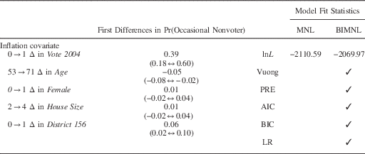
We report the complete table of outcome and inflation-stage coefficient estimates for our MNL and BIMNL models in the supplemental appendix, and focus our attention here on discussing substantive quantities of interest and model fit statistics. To begin, the left side of Table 1 reports the estimated effects of changes in each of our BIMNL model’s inflation-stage covariates upon the predicted probability of a nonvoter being an occasional, rather than routine, nonvoter.Footnote ¹⁰ In line with expectations, the BIMNL’s inflation-stage results suggest that having voted in 2004 is associated with a statistically significant 39 percent increase in a nonvoter’s likelihood of being an occasional nonvoter rather than a routine nonvoter. Similarly, and relative to District 161, nonvoters in District 156 are significantly more likely to be occasional nonvoters, perhaps owing to the higher contemporary levels of competitiveness in this district. The only significant demographic predictor of nonvoter type is age, which here implies that older nonvoters are associated with higher propensities for routine nonvoting—a relationship which may be attributable to the (likely) nonlinear effects of age in this context. The right side of Table 1 indicates that all five of our model fit statistics consistently favor the BIMNL model over the MNL model. Taken together, Table 1 provides an assortment of evidence to suggest that the BIMNL model may offer an improvement over the MNL model in modeling Arceneaux and Kolodny’s vote choice dependent variable.

Table 1

Inflation Stage and Model Fit Results for 2006 Pennsylvania (PA) Vote Choice

Note: changes in nonbinary variables=mean+1 SD changes. Values in parentheses are 90 percent confidence intervals.

MNL=multinomial logit; BIMNL=baseline-inflated multinomial logit; PRE=proportional reduction in error; AIC=Akaike information criterion; BIC=Bayesian information criterion; LR=likelihood ratio.

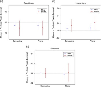
We next consider the outcome-stage vote choice estimates obtained from our MNL and BIMNL models which, as mentioned above, treat abstention as the baseline category. In deriving quantities of interest for these estimates, we hold our BIMNL inflation stage fixed at pr(noninflation=1), which enables us to directly compare our MNL model’s estimates for all individuals to the BIMNL’s hypothetical estimates for only noninflated individuals.Footnote ¹¹ This matches the claims made above, as we argued that by better accounting for routine nonvoters, the BIMNL model provides more accurate estimates of covariate effects among what is typically researchers’ primary sample of interest: occasional and routine voters. In other applications, the simultaneous effects of covariates across both stages of one’s BIMNL model may be of most interest,Footnote ¹² and these quantities (i) can also be easily derived from the probability statements in Equation (5) and (ii) have similarly been shown to exhibit less bias than comparable noninflated model quantities within extant studies of related (zero-) inflated models (Harris and Zhao Reference Harris and Zhao2007; Bagozzi et al. Reference Bagozzi and Mukherjee2015). In line with Arceneaux and Kolodny’s original study, we focus substantively on the estimated effects of 0→1 changes in both the phone and canvassing treatment on the predicted probabilities of Republican, Democrat, and Independent individuals each voting for the Democratic candidate. Given the above claims, we estimate these first differences in predicted probabilities relative to (noninflated) abstention by restricting the effects of our covariates on the other choice outcomes to zero, and plot the resultant mean estimates and confidence intervals in Figure 1.Footnote ¹³

Fig. 1

Effects of phone and canvassing on predicted probabilities of 2006 Pennsylvania (PA) vote choice Note: MNL=multinomial logit; BIMNL=baseline-inflated multinomial logit.

We begin with the Republican identifier subsample (Figure 1a). Consistent with the results reported in Arceneaux and Kolodny (Reference Arceneaux and Kolodny2009), our MNL results suggest that phone and canvassing treatments each have a significant negative effect on Republican voters’ probability of voting for the Democratic candidate. Yet, in replicating these results with the BIMNL model, we find that once routine nonvoters have been partitioned from our sample, the estimated effects of either treatment on Republican voters, although larger, are no longer statistically distinguishable from zero at traditional levels. Turning next to Independents (Figure 1b), we find that while our MNL model’s estimated effects (like those of the authors’) yield no significant findings, our BIMNL estimates for these two treatments present mean estimates that are each positive and over double in size to those of the MNL model, and which are statistically significant in the case of the phone treatment. This intuitively suggests that (i) phone treatments increase an Independent’s probability of voting Democratic and (ii) the effects of liberal endorsements on this (generally uninformed, nonpartisan) group are underestimated when routine nonvoters are unaccounted for in one’s analysis. In line with Arceneaux and Kolodny (Reference Arceneaux and Kolodny2009), we find no significant effect of either treatment among Democratic identifiers (Figure 1c), a null finding that we believe, like Arceneaux and Kolodny, may be attributable to the ceiling imposed by high levels of initial Democratic candidate support among this group. Taken together, it is not evident that liberal group endorsements are a net negative for Democratic candidate voter support (as the authors’ original findings imply), as our estimates indicate that, if anything, the net statistically distinguishable effect of these treatments is positive. Finally, one can also observe consistently larger confidence intervals for the BIMNL estimates in Figure 1, which are to be expected given that for the original BIMNL model, unlike the MNL model, one’s choice estimates are estimated conditional on estimated probabilities of inflation.

In sum, this replication provides evidence—in the form of model fit statistics and inflation-stage estimates—to suggest that the BIMNL model may outperform the MNL model in modeling the heterogeneous population of abstainers within Arceneaux and Kolodny’s vote choice dependent variable. In contrast to Arceneaux and Kolodny’s findings, our BIMNL replication suggests that liberal interest group-directed phone and door-to-door canvassing endorsements of PA Democratic House candidates now have a larger, but less precise, negative effect on Republican identifiers’ choice of voting for a Democratic candidate, and a positive (and in the case of phone treatment, significant) effect on the likelihood of Democratic candidate vote choice among Independents. In both cases, we believe that these differences are attributable to the fact that, once completely disengaged voters have been excluded, the BIMNL model is better able to estimate the effects of Arceneaux and Kolodny’s treatments upon those voters who are susceptible to such interventions. Given the substantive magnitude of our BIMNL findings for Independents, this replication has important theoretical and policy implications for interest groups’ candidate endorsement tactics, a point to which we return in the conclusion.

Replication II

Our second application replicates a recent analysis of individuals’ 2004 US presidential vote choice (Campbell and Monson Reference Campbell and Monson2008). In this study, Campbell and Monson evaluate the interactive effects of (i) gay marriage ban (GMB) ballot initiatives and (ii) potential voters’ religious affiliations on an unordered polytomous-dependent variable measuring survey respondents’ stated 2004 vote choice of: Bush, Kerry, or abstention (the baseline category). Drawing on a representative sample of ~1500 individuals from a 2004 Election Panel Study (EPS), Campbell and Monson ultimately find that the presence of GMBs increased mobilization for Bush among evangelical Protestants, but increased abstention levels (relative to voting for either candidate) among secular voters. We provide detailed operationalizations for these, and all other, covariates in our supplemental appendix.

Although Campbell and Monson’s findings are insightful, we suspect that the same heterogeneous mixture of routine nonvoters and occasional nonvoters discussed above may be present in the baseline abstention category of the authors’ polytomous dependent variable. The EPS survey likely includes substantial proportions of both types of nonvoters, given its nationally representative sample of potential voters, and given the extant literature on distinct nonvoter types (summarized earlier). If this is the case, then the authors’ estimates may be misattributing routine nonvoting effects as having direct effects on vote choice owing to heterogeneity in their nonvoting subsample of respondents. We examine whether this is the case by replicating Campbell and Monson’s primary specification using MNL and BIMNL models below.Footnote ¹⁴

As above, our choice of BIMNL inflation-stage covariates is limited to the variables available in Campbell and Monson’s study. We accordingly identify a number of plausible inflation-stage predictors from Campbell and Monson’s available covariates. First, we include education, as it has proven to be a consistent predictor of voting behavior and political participation in past research (Smets and van Ham Reference Smets and van Ham2013). We posit that educated nonvoters will have higher likelihoods of being temporary nonvoters. For similar reasons, we include the authors’ mobilization index measure, which is also anticipated to be a positive predictor of occasional, rather than routine, nonvoting. We next add Campbell and Monson’s dichotomous indicator of individuals reporting their religion as secular with the expectation that nonreligious individuals may also be less active in other areas of associational life, such as politics or voting.Footnote ¹⁵ Finally, we include age, but omit female, given the inflation-stage findings obtained in our earlier application.

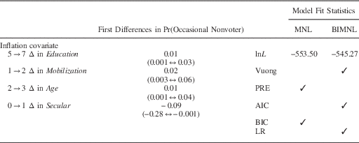
The left portion of Table 2 reports estimated changes in the predicted probabilities of noninflation (i.e., of being an occasional nonvoter rather than routine nonvoter), given reasonable changes in each of our inflation-stage covariates.Footnote ¹⁶ First, we find that a realistic increase in education is associated with a small, but significant, positive increase in a nonvoter’s likelihood of being an occasional, rather than routine, nonvoter, which is in line with our expectations. Similarly, increases in an individual’s mobilization index also positively affect the likelihood of noninflation. In contrast to our earlier application, age (now measured on a limited ordinal scale) is also a positive predictor of occasional nonvoting—a departure we find somewhat unsurprising given the different operationalizations and nonmonotonicities that likely underlie this particular relationship. Finally, secularism is associated with a large (9 percent) and significant decrease in the probability that a nonvoter is an occasional—rather than routine—nonvoter, which is consistent with our expectation that nonreligious individuals are less likely to be politically active on the whole.

Table 2

Inflation Stage and Model Fit Results for 2004 Presidential Vote Choice

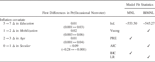
Note: changes in nonbinary variables=mean+1 SD changes. Values in parentheses are 90 percent confidence intervals.

MNL=multinomial logit; BIMNL=baseline-inflated multinomial logit; PRE=proportional reduction in error; AIC=Akaike information criterion; BIC=Bayesian information criterion; LR=likelihood ratio.

As the model fit statistics in the right portion of Table 2 reveal, we find only mixed support for the BIMNL model’s “goodness of fit” in this application. In particular, two of our three primary fit statistics favor the BIMNL model, whereas the third favors the MNL model. The less accurate PRE and Vuong statistics are similarly split between the two models. These inconclusive findings are relatively unsurprising given the low N for the study, but nevertheless underscore the need to be cautious in drawing broader theoretical conclusions from the outcome-stage results presented below.

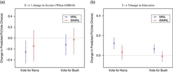
We next turn to the outcome stages of our MNL and BIMNL models. As before, the coefficient estimates for our models’ respective estimation stages are reported in the supplemental appendix. The present section compares our MNL and BIMNL derived first differences in predicted probabilities of votes for Bush and votes for Kerry,Footnote ¹⁷ given reasonable changes in two key outcome-stage covariates: secularism and education. For our BIMNL estimated first differences in predicted probabilities, we again hold the BIMNL’s inflation-stage equation fixed at pr(noninflation=1) to facilitate comparisons of our “all respondents” MNL estimates with the BIMNL model’s more specific estimated subset of “voters and occasional voters.” We report these quantities of interest, along with 90 percent confidence intervals, in Figure 2.

Fig. 2

Effects of selected covariates on predicted probabilities of 2004 vote choice Note: GMB=gay marriage ban; MNL=multinomial logit; BIMNL=baseline-inflated multinomial logit.

In addition to identifying the abstention inducing effects of GMB among secular individuals, Campbell and Monson’s reported estimates also suggest a puzzling finding, in that the individual coefficient estimate for secularism is negative and significant within the “Vote Kerry versus Abstain” equation. This implies that in states without GMB’s, secular individuals are less likely (than mainline Protestant individuals) to vote for Kerry than to abstain. As Figure 2 indicates, we find an equivalent effect in our MNL replication. However, once routine abstainers are partitioned from the sample, our comparable BIMNL estimates reveal that this effect disappears, as the estimates are now statistically indistinguishable from zero. Our estimated quantities of interest for a key control variable also highlight interesting differences between the MNL and BIMNL estimates. Specifically, the quantities of interest in Figure 2 demonstrate that a well-known positive determinate of turnout, education, has no direct effect on vote choice (relative to abstention), once its significant effects on the probability of abstention inflation are accounted for—a finding that potentially alters how we interpret the moderating effects of education within GOTV-type mobilization efforts.

In sum, our second application further highlights the benefits of the BIMNL model over the MNL model, but also underscores some potential challenges. Although we obtained a number of theoretically consistent findings for the inflation stage of our BIMNL model—such as those related to education, mobilization index, and secularism—our model fit statistics were ambiguous as to whether the BIMNL did, in fact, provide a better fit than a comparable MNL model. As such inconclusive findings are apt to occur in practice—especially when applied to data sets with fewer than 2000 observations (as was the case here)—we encourage researchers to be cautious and to rely on theory when selecting between the BIMNL and MNL model in such instances. These weak foundations notwithstanding, our outcome-stage estimates do suggest that the BIMNL model offers novel improvements in theory testing. Specifically, the puzzling estimated effect for secularism among individuals’ propensities to vote for Kerry dissipates once baseline inflation is accounted for, whereas the effect of education becomes more nuanced.

Conclusion

Questions of individual vote choice, when applied via representative surveys of voting-age citizens, are apt to include heterogeneous mixtures of nonvoters. Extant research suggests that one subset of these self-reported nonvoters will correspond to occasional nonvoters, who abstain from voting in a specific election owing to temporary factors such as short-term economic shocks, weather conditions, or personal factors. Yet, many other nonvoters are likely to be routine nonvoters who, due to structural or personal reasons, have chosen to abstain from the political process entirely. These nonvoters are thus largely immune to the short-term factors affecting the occasional abstainers mentioned above. Ignoring this distinction can lead one to conflate the estimated direct effect of both sets of determinants on nonvoting and, by implication, the factors affecting actual voters’ candidate choices in MNL models. Hence, it is imperative that public opinion scholars account for these disparate populations of nonvoters when “did not vote/abstain” serves as the reference category in empirical models of vote choice.

This paper presents a new discrete choice estimator—the BIMNL model—to allow researchers to more accurately account for this variation in populations of nonvoters. After deriving this model, we demonstrate that ignoring baseline-choice category inflation within empirical studies of vote choice can potentially affect one’s parameter estimates and theoretical conclusions. Here, our replication findings offer new theoretical insights into the determinants of individual vote choice in American elections. For instance, our first application demonstrates that the effects of a liberal interest group’s Democratic candidate endorsement may in fact produce a net positive, rather than a net negative, outcome for Democratic candidates across all potential voters, once routine nonvoters are accounted for in the BIMNL model. Similarly, our second application suggests that a number of commonly understood direct predictors of turnout and vote choice, such as education and secularism, may instead primarily affect these outcomes through their effects on routine versus occasional nonvoting, rather than through any direct effect on individuals’ active decisions to vote or abstain in a given election.

This study can be extended in several directions. As mentioned above, the BIMNL model could be generalized to the MNP setting. Notwithstanding the MNP concerns raised earlier, such an extension would afford researchers the opportunity to properly account for baseline category inflation in instances where they believe their polytomous dependent variable to be both unordered and in broader violation of the IIA assumption. Furthermore, a BIMNP model could also provide a feasible framework for the provision of correlated error terms between the two estimation stages of an inflated polytomous choice model (under assumptions of bivariate normality). Allowances for correlated disturbances between inflation and outcome equations, although challenging for estimation and identification, have been shown to be extremely useful to both theory and estimation within inflated ordered probit estimators (Harris and Zhao Reference Harris and Zhao2007; Bagozzi and Mukherjee Reference Bagozzi, Hill, Moore and Mukherjee2012; Bagozzi et al. Reference Bagozzi and Mukherjee2015), as well as in applications of inflated probit estimators (e.g., Xiang Reference Xiang2010), and thus would likely be of great interest to survey researchers within the polytomous choice setting as well.

The insights presented above may also facilitate future research within the area of political behavior by allowing researchers to better test and develop theories of routine and occasional nonvoting. As such, our paper has important implications for political behavior research both within academia as well as in the more applied settings of political campaigns and activism. By accounting for routine nonvoters, the BIMNL model provides more nuanced estimates of how various factors affect the voting behavior of the very individuals that campaigns and scholars (arguably) want to understand and motivate the most: those who have voted in past elections but not necessarily routinely. It is this population of disproportionately nonpartisan, uninformed, and heuristic-dependent (non)voters who, if effectively mobilized, can have a substantively large effect on an electoral outcome. As the 2008 election demonstrated, the ability to encourage voter turnout among populations of Americans with inconsistent voting records (e.g., young voters between the ages of 18 and 29) can significantly bolster support for one party, or candidate, over another. Thus, accurately understanding how GOTV activities differentially affect occasional versus routine nonvoters could be crucial for many political campaigners, interest organizations, and scholars of political behavior.