





1. Introduction
Modelling the boundary region of magnetically confined fusion plasmas remains a challenge for the fusion community. Fluctuations at all scales need to be considered, as well as kinetic effects and collisional processes. Developing a model for simulating the plasma boundary requires overcoming the limitations of existing models. Full-f fluid codes focus on the long-wavelength limit (Paruta et al. Reference Paruta, Ricci, Riva, Wersal, Beadle and Frei2018; Giacomin et al. Reference Giacomin, Ricci, Coroado, Fourestey, Galassi, Lanti, Mancini, Richart, Stenger and Varini2022; De Lucca et al. Reference De Lucca, Ricci, Bassanini, García Herreros and Tecchiolli2026), and their validity is limited to the highly collisional regime. Gyrofluid codes apply Padé approximation to relax the long-wavelength approximation (Held, Wiesenberger & Kendl Reference Held, Wiesenberger and Kendl2020; Held & Wiesenberger Reference Held and Wiesenberger2022). Additionally, they use kinetic closures to avoid considering the highly collisional limit, although the success of these closures is highly case dependent (Beer & Hammett Reference Beer and Hammett1996; Wiesenberger & Held Reference Wiesenberger and Held2022, Reference Wiesenberger and Held2024). However, gyrokinetic (GK)
 $\delta$
-f models, which offer a good description of the core of fusion plasmas (Jenko et al. Reference Jenko, Dorland, Kotschenreuther and Rogers2000; Pan, Told & Jenko Reference Pan, Told and Jenko2016), present the challenge of including collisions at the level of relevance for the boundary. Furthermore, their application to the boundary is questionable due to large-scale fluctuations present in this region. Full-f GK codes often focus on the long-wavelength limit (Chang et al. Reference Chang2017; Dorf & Dorr Reference Dorf and Dorr2020; Hakim et al. Reference Hakim, Mandell, Bernard, Francisquez, Hammett and Shi2020; Michels et al. Reference Michels, Ulbl, Zholobenko, Body, Stegmeir, Eich, Griener, Conway and Jenko2022; Ulbl et al. Reference Ulbl, Body, Zholobenko, Stegmeir, Pfennig and Jenko2023) and thus compromise physical fidelity at the cost of computational performance.
To overcome the limitations of these approaches and accurately describe the boundary, Qin et al. (Reference Qin, Cohen, Nevins and Xu2006), Hahm, Wang & Madsen (Reference Hahm, Wang and Madsen2009) and Frei, Jorge & Ricci (Reference Frei, Jorge and Ricci2020) propose a model that couples a drift-kinetic (DK) and GK ordering. Here, we leverage the single-particle one-form derived by Frei et al. (Reference Frei, Jorge and Ricci2020), and present a first implementation of a model that couples DK and GK orderings. The single-particle one-form is derived by first performing a guiding-centre transformation, yielding the DK part of the single-particle one-form, and a consequential gyrocentre transformation, yielding the GK part of the single-particle one-form. In the literature, guiding-centre and DK and, likewise, gyrocentre and GK are used interchangeably. More precisely, this work relies on splitting the distribution functions into a DK large-scale slowly varying part and a GK small-scale rapidly varying part. The DK fields are allowed to be large in amplitude but only vary on long scale, employing a long-wavelength limit, while the GK fields are small in amplitude but allowed to vary on all scales.
The model is based on single particle equations of motion derived from first principles starting from the particle one-form. From the single particle equations of motion, the gyro-averaged Boltzmann equation is derived, split into a GK part and a DK part, and projected onto a Hermite–Laguerre basis giving a DK and a GK hierarchy equation for the projection coefficients, denoted as gyromoments. The Hermite–Laguerre projection allows for an efficient implementation of the plasma dynamics, including multiple different collision operators. Finally, we split the electrostatic potential into a DK part and a GK part, similarly to the distribution functions, and we derive a DK and GK Poisson equation from first principles by using a variational principle.
Previous
 $\delta$
-f GK gyromoment simulations based on the Hermite–Laguerre projection are shown to efficiently reduce the computational complexity of solving the GK system of equations compared with continuum
 $\delta$
-f GK simulations (Hoffmann et al. Reference Hoffmann, Frei and Ricci2023a
,
Reference Hoffmann, Frei and Riccib
; Mandell et al. Reference Mandell, Dorland, Abel, Gaur, Kim, Martin and Qian2024). Similarly, full-f gyromoment simulations were performed in a linear plasma device, within a DK ordering (Frei, Mencke & Ricci Reference Frei, Mencke and Ricci2024; Mencke & Ricci Reference Mencke and Ricci2025). This work combines the advantages of the two previously developed models allowing for order-one DK fluctuations with small wavenumbers and, at the same time, small-amplitude GK fluctuations with arbitrary wavenumbers. It then enables the study of instabilities on all scales, while still removing the single-particle gyromotion from the description.
Although our approach ultimately is intended for the boundary of magnetically confined fusion devices, we consider the simpler case of a linear plasma device in this work. A linear plasma device offers an ideal testbed for new global turbulent plasma simulations. The absence of drifts associated with the curvature of the magnetic field, together with the smaller size of the simulations compared with toroidal devices, reduces the complexity and cost of the simulations, and allows for a deeper understanding of the physics at play (Friedman et al. Reference Friedman, Carter, Umansky, Schaffner and Dudson2012). We note that despite their simple geometries, previous simulations of linear plasma devices show complex turbulent behaviour (Popovich et al. Reference Popovich, Umansky, Carter and Friedman2010; Rogers & Ricci Reference Rogers and Ricci2010; Pan et al. Reference Pan, Told and Jenko2016, Reference Pan, Told, Shi, Hammett and Jenko2018; Shi et al. Reference Shi, Hammett, Stoltzfus-Dueck and Hakim2017; Frei et al. Reference Frei, Mencke and Ricci2024; Mencke & Ricci Reference Mencke and Ricci2025). Finally, the perpendicular incidence of the magnetic field with the walls at the end of the plasma column simplify the boundary conditions of the simulations.
This paper is structured as follows. In § 2, we present the ordering used as well as the equations describing the evolution of the distribution functions. The DK model for the ions and electrons is derived in § 3 from a kinetic description, and similarly, the GK model is derived in § 4. We close the system in § 5 by deriving the DK and GK Poisson equations used to solve for the two electrostatic potentials. The numerical implementation of the physical model is described in § 6. In § 7, we report the results of the comprehensive turbulent simulations comparing it with a full-f DK simulation where the GK perturbations are suppressed. Section 8 provides an analysis of the findings in § 7 by presenting linear investigations of the turbulence-driving instabilities. Finally, the conclusions follow in § 9.
2. Ordering assumptions and equations of motion
We focus on the case of a fully ionised plasma with one single-ionised ion species such that the plasma is composed of species
 $a=i,e$
with
 $e$
denoting the electrons and
 $i$
the only ion species with charge
 $q_i=e$
. We split the electrostatic potential
 \begin{align} \phi \left (\boldsymbol{x}\right )= \phi _{DK}\left (\boldsymbol{x}\right )+\phi _{GK}\left (\boldsymbol{x}\right ), \end{align}
where
 $\boldsymbol{x}$
is the particle position, and we impose that the GK part of the electrostatic potential has a small amplitude compared with the DK part,
 $\phi _{GK}/\phi _{DK}\sim \epsilon _{\delta }\lt 1$
. We order the DK and GK quantities such that they vary on different length scales. More precisely, we order the perpendicular gradient lengths,
 $k_{\perp DK}\sim \left |\boldsymbol{\nabla} _{\perp } \ln F_{aDK}\right |\sim \left |\boldsymbol{\nabla} _{\perp } \ln \phi _{DK} \right |\sim \epsilon _{\perp }/\rho _s$
with
 $\epsilon _{\perp }\lt 1$
and
 $k_{\perp GK}\sim \left |\boldsymbol{\nabla} _{\perp } \ln \phi _{GK} \right |\sim 1/\rho _s$
, being
 $\rho _s=c_s/\varOmega _i$
the ion sound Larmor radius with
 $c_s=\sqrt {T_e/m_i}$
the sound speed,
 $T_e$
the electron temperature and
 $\varOmega _i=q_i B/m_i$
the ion gyro frequency, with
 $B$
the magnetic field strength. Furthermore, we order the parallel length scale as
 $k_{\parallel }\sim \epsilon k_{\perp DK}$
and the frequency as
 $\omega \sim \varOmega _i \epsilon \epsilon _{\perp }$
. This ordering imposes that
 $\phi _{DK}$
gives a contribution to the
 $\boldsymbol E \times \boldsymbol B$
velocity of the order of
 $\epsilon _{\perp }/\epsilon _{\delta }$
with respect to that of
 $\phi _{GK}$
(Frei et al. Reference Frei, Jorge and Ricci2020). By further ordering
 $\epsilon _{\perp }\sim \epsilon _{\delta }$
, we impose that the
 $\boldsymbol E \times \boldsymbol B$
drift from the DK electrostatic potential contributes to the drifts, comparably to the GK counterpart. We note that in the following, we consider a linear plasma device where
 $\boldsymbol B$
is a constant and therefore also
 $B$
.
Based on this ordering, we derive the single-particle dynamics in § 2.1. The behaviour of the full distribution function is described in § 2.2 using the Boltzmann equation. Finally, the evolution of the DK and GK parts of the distribution function is derived from the Boltzmann equation in § 2.3.
2.1. Single-particle dynamics
We assume that the collisionless particle dynamics be governed by the gyrocentre single-particle Lagrangian,
 $\varGamma _A$
. By using a Lie approach and including all terms up to second order in the GK and DK parts of the
 $\boldsymbol E \times \boldsymbol B$
drift (i.e. to order
 $c_s^2 \epsilon _{\perp }^2$
and
 $c_s^2 \epsilon _{\delta }^2$
), while assuming a straight and constant magnetic field, we have (Frei et al. 2020)
 \begin{align} \varGamma _a(\boldsymbol R, \mu , v_\parallel ,t)= q_a \boldsymbol A_a^* \boldsymbol{\cdot }\,\dot {\!\boldsymbol R} - \frac {\mu B}{\varOmega _i} \dot \theta - m_a v_\parallel ^2 / 2-\mu B - q_a \varPhi _a^*+\mathcal{O}\!\left (\frac {m_a}{m_i}T_a\epsilon _{\perp }^3,\frac {m_a}{m_i}T_a\epsilon _{\delta }^3\right ),\nonumber\\[1pt] \end{align}
where
 $v_{\parallel }=\boldsymbol{v}\boldsymbol{\cdot }\boldsymbol{b}$
is the velocity component parallel to the magnetic field,
 $\boldsymbol{b}$
is the unit vector in the direction of the magnetic field,
 $\mu = m_a v_{\perp }^2/B$
is the adiabatic invariant,
 $m_a$
is the mass of species
 $a$
and
 $v_{\perp }=\left |\boldsymbol{v}-\boldsymbol{b}v_{\parallel }\right |$
is the velocity component perpendicular to the magnetic field. We also define the fields
 $q_a \varPhi _a^* =q_a \phi _{DK} +q_a \varPhi _E+q_a\psi _{GK}$
and
 $q_a \boldsymbol A_a^* = q_a {\boldsymbol A} + m_a v_\parallel \boldsymbol b+m_a \boldsymbol u_{E}$
, where
 $q_a\varPhi _E=m_a\left |\boldsymbol u_E\right |^2/2+\mu B \boldsymbol{\nabla} _{\perp }^2\phi _{DK} /\left (2 B \varOmega _a \right )$
and
 $\boldsymbol u_E=-\boldsymbol{\nabla }\phi _{DK} \times \boldsymbol B/B^2$
is the
 $\boldsymbol E \times \boldsymbol B$
velocity for the DK potential. The effective GK gyro-averaged potential is defined as
 \begin{align} \psi _{GK} =\left \langle \phi _{GK}\right \rangle _{{\boldsymbol R}}+\frac {q_a^2}{2m_a\varOmega _a}\partial _{\mu }\left (\left \langle \phi _{GK}\right \rangle _{{\boldsymbol R}}^2-\left \langle \phi _{GK}^2\right \rangle _{{\boldsymbol R}}\right )+\frac {q_a}{2m_a \varOmega _a^2}\left \langle \left (\boldsymbol{b}\times \boldsymbol{\nabla }\overline {\widetilde {\phi _{GK}}}\right )\boldsymbol{\cdot }\boldsymbol{\nabla }\widetilde {\phi _{GK}}\right \rangle _{{\boldsymbol R}}, \end{align}
where the gyroaverage operator is introduced,
 \begin{align} \left \langle f\right \rangle _{{\boldsymbol R}}&=\frac {1}{2 \pi } \int _0^{2 \pi } \mathrm{d} \theta \int \mathrm{d} \boldsymbol{x} \delta ({\boldsymbol{R}}+\boldsymbol{\rho }_a-\boldsymbol{x}) f(\boldsymbol{x}, {\mu }, {v}_{\parallel }, t)\\[-10pt]\nonumber \end{align}
 \begin{align} &=\frac {1}{2 \pi } \int _0^{2 \pi } \mathrm{d} \theta \sum _{n=0}^{\infty } \frac {\left (\boldsymbol{\rho }_a\boldsymbol{\cdot }\boldsymbol{\nabla }\right )^n}{n!}f(\boldsymbol{R}, {\mu }, {v}_{\parallel }, t)\\[-10pt]\nonumber \end{align}
 \begin{align} &=\sum _{n=0}^{\infty }\left (\frac {2\mu }{q_a\varOmega _a}\right )^{n}\frac {\boldsymbol{\nabla} _{\perp }^{2n}}{2^n n!n!}f(\boldsymbol{R}, {\mu }, {v}_{\parallel }, t), \end{align}
with
 $\delta \left (\boldsymbol{\cdot }\right )$
the Dirac delta function and
 $\boldsymbol{\rho }_a=\boldsymbol{a}v_{\perp }/\varOmega _a$
, the Larmor radius, being
 $\boldsymbol{a}$
a unit vector perpendicular to both the magnetic field and the gyromotion of the particle (Frei et al. Reference Frei, Jorge and Ricci2020). Finally, we define
 \begin{align} \widetilde {\phi _{GK}}&=\phi _{GK}-\left \langle \phi _{GK}\right \rangle _{{\boldsymbol R}} \end{align}
and
 \begin{align} \overline {\widetilde {\phi _{GK}}}&= \int ^\theta {\rm d}\theta ^\prime \widetilde {\phi _{GK}}(\boldsymbol{x}(\boldsymbol R,\theta ^\prime ), {\mu }, {v}_{\parallel }, t) \end{align}
in (2.3).
We note that the Lagrangians that describe this system are given by
 \begin{align} L_a=F_a\varGamma _a, \end{align}
and for the evolution of the distribution functions, we use (2.6) to the lowest order in
 $\epsilon _{\perp }$
, i.e. we neglect the
 $\sim \boldsymbol{\nabla} _\perp ^2 \phi _{DK}$
and
 $\sim \left |\boldsymbol u_E\right |^2$
terms that ensure accuracy to order
 $T_e\epsilon _{\delta }^2$
and
 $T_e\epsilon _{\perp }^1$
. However, to ensure that the long-wavelength radial electric field (i.e.
 $-\partial _r\phi _{DK}$
) is properly modelled, we include these terms when we derive a quasineutrality condition (Parra & Catto Reference Parra and Catto2008, Reference Parra and Catto2010).
2.2. Collective behaviour
The collective behaviour of the distribution function is governed by the gyroaveraged Boltzmann equation (Frei et al. Reference Frei, Jorge and Ricci2020),
 \begin{align} \partial _t F_a+\dot {{\boldsymbol R}}\boldsymbol{\cdot }\boldsymbol{\nabla }F_a +\dot {v}_{\parallel }\partial _{v_{\parallel }} F_a = \left \langle S_{a}\right \rangle _{{\boldsymbol R}}+ \sum _{b=i,e}\left \langle C_{ab}\right \rangle _{{\boldsymbol R}}, \end{align}
where the sources for species
 $a$
,
 $S_a$
, are introduced along with the collision operator between species
 $a$
and
 $b$
,
 $C_{ab}$
, and the parallel acceleration,
 $\dot {v_{\parallel }}$
.
The Euler–Lagrange equations of the ion Lagrangian, (2.2), give
 \begin{align} v_{\parallel } &=\boldsymbol b \boldsymbol{\cdot }\dot {{\boldsymbol R}},\\[-10pt]\nonumber \end{align}
 \begin{align} \dot {\mu }&=0,\\[-10pt]\nonumber \end{align}
 \begin{align} -q_a \boldsymbol B^*\times \dot {{\boldsymbol R}}-m_a \dot {v}_{\parallel }\boldsymbol b&=q_a\boldsymbol{\nabla }\varPhi ^*_a+q_a\partial _t \boldsymbol A^*, \end{align}
introducing the effective magnetic field,
 $\boldsymbol{B}^*=\boldsymbol{\nabla }\times \boldsymbol{A}^*$
. Now, projecting (2.8c
) on the
 $\boldsymbol{B}^*$
direction and crossing with
 $\boldsymbol b$
, we obtain respectively
 \begin{align} \dot {v}_{\parallel } B_{\parallel }^{*}&=-\frac {q_a}{m_a} \boldsymbol B^*\boldsymbol{\cdot }(\boldsymbol{\nabla }\varPhi ^*_a+\partial _t\boldsymbol A^*),\\[-10pt]\nonumber \end{align}
 \begin{align} \dot {{\boldsymbol R}}B_{\parallel }^{*}&=\boldsymbol B^* v_{\parallel }+\boldsymbol b\times (\boldsymbol{\nabla }\varPhi ^*_a+\partial _t \boldsymbol A^*), \end{align}
where
 $B_{\parallel }^{*}=\boldsymbol{B}^*\boldsymbol{\cdot }\boldsymbol b$
. Equations (2.9a
) and (2.9b
) are used to evolve the distribution functions through the Boltzmann equation. Equation (2.9a
) describes the parallel acceleration of particles subject to an effective magnetic field,
 $\boldsymbol B^*$
, and an effective electric field,
 $\boldsymbol E^*=\boldsymbol{\nabla }\varPhi _a^*+\partial _t \boldsymbol A^*$
, where
 $B_{\parallel }^{*}$
describes the Jacobian of the coordinate transform from particle position to gyrocentre position. Similarly, (2.9b
) describes the gyrocentre motion as the sum of a parallel drift term and an
 $\boldsymbol E \times \boldsymbol B$
-drift term with the effective magnetic and electric field,
 $\boldsymbol B^*$
and
 $\boldsymbol E^*$
(Qin et al. Reference Qin, Cohen, Nevins and Xu2006; Hahm et al. Reference Hahm, Wang and Madsen2009; Frei et al. Reference Frei, Jorge and Ricci2020).
Considering the lowest order in
 $m_e/m_i$
in (2.2), the electron one-form becomes
 \begin{align} \varGamma _e(\boldsymbol R, \mu , v_\parallel ,t) & = (q_e \boldsymbol A+m_ev_{\parallel }\boldsymbol b) \boldsymbol{\cdot }\,\dot {\!\boldsymbol R} - \frac {\mu B}{\varOmega _e} \dot \theta - m_e v_\parallel ^2 / 2\nonumber\\[3pt]& \quad -\mu B - q_e \left (\phi _{DK}+\phi _{GK}\right )+\mathcal{O}\left (\frac {m_e}{m_i}T_a\right ), \end{align}
with the equations of motion identical to that of the ions in (2.9), with
 $B_{\parallel }^{*}=B$
,
 $m_a=m_e$
,
 $\varPhi _e^*=\phi _{DK}+\phi _{GK}$
,
 $\boldsymbol B^*=\boldsymbol B$
and
 $\partial _t\boldsymbol A^*=0$
.
In the following, we apply ordering arguments to the equations of motion in (2.9). This breaks the inherent conservative properties ensured by a variational approach arising from the symmetries in the Lagrangian; however, it greatly simplifies the numerical implementation of the resulting model.
2.3. DK and GK Boltzmann equations
Given the equations of motion in (2.9), equation (2.7) can, in principle, be solved with appropriate numerical methods once the sources,
 $S_a$
, collision operators,
 $C_{ab}$
, and electrostatic potentials,
 $\phi _{DK}$
and
 $\phi _{GK}$
, are defined. However, we rely, in the following, on the splitting of the distribution function in a similar way as
 $\phi$
in (2.1). That is,
 \begin{align} F_a(\boldsymbol{R},v_{\parallel }, \mu )= F_{aDK}(\boldsymbol{R},v_{\parallel }, \mu )+F_{aGK}(\boldsymbol{R},v_{\parallel }, \mu ). \end{align}
Analogously to the electrostatic potential, we impose
 $F_{aGK}\sim \epsilon _{\delta }F_{aDK}$
,
 $\left |\boldsymbol{\nabla} _\perp \ln F_{aDK}\right |\sim k_{\perp DK}$
and
 $\left |\boldsymbol{\nabla} _\perp \ln F_{aGK}\right |\sim k_{\perp GK}\sim 1/\rho _s$
.
In the following, we use an ordering argument in
 $\epsilon _\perp$
to significantly simplify the evolution equations for
 $F_{aDK}$
and
 $F_{aGK}$
. We note that the higher order terms in
 $\epsilon _\perp$
in the single-particle one-form, (2.2), and the resulting single-particle drifts and accelerations, (2.9), are strictly necessary for the quasi-neutrality condition as a direct consequence of the intrinsic ambipolarity of the electrostatic potential. As we show in § 5, the evolution of the DK polarisation density
 $\sim \boldsymbol{\nabla} _\perp \boldsymbol{\cdot }\left (N_{iDK}\boldsymbol{\nabla} _\perp \phi _{DK}\right )\sim N_{iDK}\epsilon _\perp ^2$
requires knowledge of the electron and ion DK density difference to order
 $\epsilon _\perp ^2$
higher than the evolution of the electron and ion DK densities. Therefore, in §§ 3 and 4, we only include the lowest order drifts and accelerations in
 $\epsilon _\perp$
to evolve
 $F_{aDK}$
and
 $F_{aGK}$
.
To separate the DK and GK part of the distribution function, we average (2.7) over small scales, defining the averaging operator such that for any DK-ordered field,
 $g_{aDK}$
,
 \begin{align} \left \langle g_{aDK}\right \rangle _{DK}&=g_{aDK}, \end{align}
and for the GK fields,
 \begin{align} \left \langle F_{aGK}\right \rangle _{DK}&=0,\\[-6pt]\nonumber \end{align}
 \begin{align} \left \langle \boldsymbol{\nabla} _{\perp } \left \langle \phi _{GK}\right \rangle _{{\boldsymbol R}}\right \rangle _{DK}&=\boldsymbol{\nabla} _{\perp }\phi _{GK},\\[-6pt]\nonumber \end{align}
 \begin{align} \left \langle \boldsymbol{\nabla} _{\parallel } \left \langle \phi _{GK}\right \rangle _{{\boldsymbol R}}\right \rangle _{DK}&=0, \end{align}
with
 $\boldsymbol{\nabla} _{\parallel }=\boldsymbol b \boldsymbol{\cdot }\boldsymbol{\nabla}$
. The averaging operation removes all fluctuations on the Larmor-radius scale and we assume that only the perpendicular electric field has a large-scale component due to the assumption
 $\boldsymbol{\nabla} _{\perp }\phi _{DK}\sim \boldsymbol{\nabla} _{\perp }\phi _{GK}$
. The leading order (in
 $\epsilon _\perp$
) DK average of (2.7) is
 \begin{align} \partial _t F_{aDK}&+\boldsymbol{\nabla }\boldsymbol{\cdot }\left (\,\dot {\!\boldsymbol R}_{DK} F_{aDK}\right )+\dot {v}_{\parallel DK}\partial _{v_{\parallel }} F_{aDK} = S_{aDK}+ \sum _{b=i,e}C_{ab DK}+\mathcal{O}\left (F_{a}\varOmega _i\epsilon \epsilon _{\perp }^2\right ), \end{align}
where
 \begin{align} \,\dot {\!\boldsymbol R}_{DK}&=\boldsymbol b v_{\parallel }+\frac {1}{B}\boldsymbol b\times \boldsymbol{\nabla }\left (\phi _{DK}+\phi _{GK}\right ),\quad \dot {v}_{\parallel DK}=-\frac {q_a}{m_a}\boldsymbol{\nabla} _{\parallel }\phi _{DK},\\[-8pt]\nonumber \end{align}
 \begin{align} S_{aDK}&=\left \langle S_a\right \rangle _{DK},\quad C_{abDK}=\left \langle C_{ab}\right \rangle _{DK}=C_{ab}\left (F_{aDK},F_{bDK}\right ), \end{align}
and we have used that
 $\boldsymbol{\nabla }\boldsymbol{\cdot }\,\dot {\!\boldsymbol R}_{DK}=0$
.
Finally, the GK Boltzmann equation is retrieved by subtracting (2.13a ) from (2.7). That is,
 \begin{align} \partial _t F_{aGK}&+\boldsymbol{\nabla }\boldsymbol{\cdot }\left (\left (\,\dot {\!\boldsymbol R}-\,\dot {\!\boldsymbol R}_{DK}\right ) F_{aDK}+\,\dot {\!\boldsymbol R} F_{GK}\right )+\dot {v}_{\parallel DK}\partial _{v_{\parallel }} F_{aGK}+ \dot {v}_{\parallel GK}\partial _{v_{\parallel }} F_{aDK}\nonumber \\[3pt] &= \left \langle S_{a}\right \rangle _{{\boldsymbol R}}-S_{aDK}+ \sum _{b=i,e}\left (\left \langle C_{ab}\right \rangle _{{\boldsymbol R}}-C_{ab DK}\right )+\mathcal{O}\left (F_{a}\varOmega _i\epsilon \epsilon _{\perp }^2\epsilon _{\delta }\right ), \end{align}
with
 \begin{align} \dot {v}_{\parallel GK}&=-\frac {q_a}{m_a}\boldsymbol{\nabla} _{\parallel }\left \langle \phi _{GK}\right \rangle _{{\boldsymbol R}} \end{align}
and
 $\boldsymbol{\nabla }\boldsymbol{\cdot }\,\dot {\!\boldsymbol R}=\mathcal{O}\left (\epsilon \epsilon _\perp ^2\epsilon _\delta \right )$
.
Equations (2.13a
) and (2.14a
) describe the evolution of the distribution functions given the electrostatic potentials,
 $\phi _{DK}$
and
 $\phi _{GK}$
.
3. Drift-kinetic governing equations
This section presents the derivation of the part of the model that governs the dynamics of the distribution functions on the DK scale. We simplify the electron evolution described by the DK Boltzmann (2.13a ) using the ordering in § 3.1. Furthermore, also starting from (2.13a ), we derive a gyromoment hierarchy equation for the ions in § 3.2 by expanding the ion distribution function on a Hermite–Laguerre basis.
3.1. Electron drift-kinetic model
For the electrons, we notice that the leading order term in (2.13a
) is order
 $F_{a}\varOmega _i\epsilon \epsilon _{\perp }\sqrt {m_i/m_e}$
. Expanding the electron distribution function in terms of the square root of the mass ratio and keeping terms only to first order,
 $F_{eDK}=F_{eDK0}+F_{eDK1}$
, with
 $F_{eDK1}\sim \epsilon _m F_{eDK0}$
and
 $\epsilon _m=\sqrt {m_e/m_i}$
, the lowest order terms appearing in (2.13a
) are
 \begin{align} v_{\parallel }\boldsymbol{\nabla} _{\parallel } F_{eDK0}&+\frac {e}{m_e}\boldsymbol{\nabla} _{\parallel }\phi _{DK}\partial _{v_{\parallel }} F_{eDK0}=C_{ee}\left (F_{eDK0},F_{eDK0}\right )+C_{ei}\left (F_{eDK0},F_{iDK}\right ), \end{align}
where
 $C_{ei}$
, at leading order in
 $\epsilon _m$
, is given by (Braginskii Reference Braginskii1965)
 \begin{align} C_{ei}\left (F_{eDK}, F_{iDK}\right )&=-\frac {L_{ei}N_{eDK}}{8\pi }\partial _{v_{\gamma }}\left (V_{\beta \gamma }\partial _{v_{\beta }}F_{eDK}\right ) =\mathcal{L}_{ei}\left (F_{eDK}\right ) , \end{align}
with
 \begin{align} L_{ei}&=\frac {3\sqrt {\pi }}{4}\frac {\nu _{ei}}{N_{eDK}}v_{Th e}^3,\quad v_{Th e}=\sqrt {\frac {2 T_e}{m_e}},\\[-10pt]\nonumber \end{align}
 \begin{align} V_{\beta \gamma }&=\frac {1}{v^3}\left (v^2 \delta _{\beta \gamma }-v_{\beta }v_{\gamma }\right ),\quad N_{eDK}=\int {\rm d}\boldsymbol v F_{eDK}. \end{align}
A solution of (3.1a ) is given by
 \begin{align} F_{eDK0}&=N_{eDK0}\left (\boldsymbol{R},t\right )\frac {m_e^{3/2}}{\left (2\pi T_{eDK0}\left (\boldsymbol{R}_\perp ,t\right )\right )^{3/2}}\exp \left (-\frac {m_ev^2}{2T_{eDK0}\left (\boldsymbol{R}_\perp ,t\right )}\right ),\\[-6pt]\nonumber \end{align}
 \begin{align} N_{eDK0}\left (\boldsymbol{R},t\right )&=N_{e\perp }\left (\boldsymbol{R}_\perp ,t\right )\exp \left (\frac {e\phi _{DK}\left (\boldsymbol{R},t\right )}{T_{eDK0}\left (\boldsymbol{R}_\perp ,t\right )}\right ), \end{align}
where
 $\boldsymbol{R}_\perp \equiv \boldsymbol b\times \left (\boldsymbol R\times \boldsymbol b\right )$
refers to the spatial coordinates perpendicular to the magnetic field and
 $T_{eDK0}$
corresponds to the temperature of the Maxwellian
 $F_{eDK0}$
. We note that the Maxwellian velocity dependency of
 $F_{eDK0}$
ensures that the right-hand side of (3.1a
) vanishes while the spatial dependence of
 $\boldsymbol b\boldsymbol{\cdot }\boldsymbol R$
through
 $N_{eDK0}$
ensures that the left-hand side of (3.1a
) vanishes. To obtain an evolution equation for
 $N_{eDK0}$
and
 $T_{eDK0}$
, we consider the next order in
 $\epsilon _m$
of the Boltzmann equation, (2.13a
), that is,
 \begin{align} \partial _t F_{eDK0}&+\frac {1}{B} \left [\phi _{DK}+\phi _{GK}, F_{eDK0} \right ]+v_{\parallel }\boldsymbol{\nabla} _{\parallel } F_{eDK1}+\frac {e}{m_e}\boldsymbol{\nabla} _{\parallel }\phi _{DK}\partial _{v_{\parallel }} F_{eDK1}\nonumber \\ &=C_{ee}^{\left (1\right )}\left (F_{eDK1}\right )+\mathcal{L}_{ei}\left (F_{eDK1}-\frac {m_e v_{\parallel } J_{\parallel }}{N_{eDK0}T_{eDK0}} F_{e0}\right )+S_{eDK}, \end{align}
with
 $ \left [f, g \right ]=\boldsymbol b\boldsymbol{\cdot }\boldsymbol{\nabla }f \times \boldsymbol{\nabla }g$
. The
 $F_{eDK1}$
that solves (3.3) is
 \begin{align} F_{eDK1}&=\left [\frac {N_{e1}}{N_{eDK0}}+\frac {P_{e1}}{N_{eDK0}T_{eDK0}}\left (\frac {m_ev^2}{2T_{eDK0}}-\frac {3}{2}\right )\right ]F_{eDK0}+f_{sh}, \end{align}
where
 \begin{align} f_{sh}&=\sum _{k=0}^{\infty }v_{\parallel } \frac {F_{eDK}}{N_{eDK0}} A_k(\boldsymbol R) L_{k}^{3/2}\left (m_ev^2/2T_{eDK0}\right ). \end{align}
Truncating
 $f_{sh}$
at
 $k=3$
, we determine
 $A_k$
, as described in Appendix A, obtaining
 \begin{align} A_0&=2\frac {m_e}{T_{eDK0}}N_{eDK0}U_{\parallel e DK},\quad A_1 =1.266 C_{P1}+0.286\frac {m_e}{T_e} J_{\parallel },\\[-10pt]\nonumber \end{align}
 \begin{align} A_2&= -0.654 C_{P1}+0.055 \frac {m_e}{T_e} J_{\parallel },\quad A_3=0.0193 C_{P1}+0.0238 \frac {m_e}{T_e} J_{\parallel }, \end{align}
being
 \begin{align} C_{P1}&=\frac {1}{T_{eDK0}\nu _{ee}}\boldsymbol{\nabla} _{\parallel }T_{e1}\quad \text{and}\quad T_{e1}= \frac {P_{e1}}{N_{eDK0}}. \end{align}
By taking the moments of (3.3) with weight
 $1$
and
 $m_ev^2/2$
, we determine an evolution equation for
 $N_{eDK}=N_{eDK0}+N_{e1}$
and
 $T_{eDK}=T_{eDK0}+T_{e1}$
, respectively, that is,
 \begin{align} &\partial _t N_{eDK}+\frac {1}{B} \left [\phi _{DK}+\phi _{GK}, N_{eDK} \right ]+\boldsymbol{\nabla} _{\parallel }\left (U_{\parallel eDK}N_{eDK}\right )=S_N+\mathcal{O}\left (N_{e}\varOmega _i\epsilon \epsilon _{\perp }^3\right ) \end{align}
and
 \begin{align} &\frac {3}{2}\left (\partial _t T_{eDK}+\frac {1}{B} \left [\phi _{DK}+\phi _{GK}, T_{eDK} \right ]+U_{\parallel eDK}\boldsymbol{\nabla} _{\parallel }T_{eDK}\right )\nonumber \\[5pt] &+T_{eDK}\boldsymbol{\nabla} _{\parallel } U_{\parallel eDK}-\frac {0.71 T_{eDK}}{N_{eDK}}\boldsymbol{\nabla} _{\parallel }J_{\parallel }+\frac {1}{N_{eDK}}\boldsymbol{\nabla} _{\parallel }q_{\parallel e r}=\frac {3}{2}S_{Te}+\mathcal{O}\left (T_{e}\varOmega _i\epsilon \epsilon _{\perp }^3\right ), \end{align}
being
 \begin{align} q_{\parallel e r}&=-\frac {3.16N_{eDK}T_{eDK}}{m_e\nu _{ee}}\boldsymbol{\nabla} _{\parallel }T_{eDK}, \end{align}
(see Appendix A for the details of the derivation). We note that (3.5a
) and (3.5b
) correspond to the evolution of the density and electron temperature in the drift-reduced Braginskii model with the electrostatic potential expressed as the sum of the GK and DK electrostatic potentials,
 $\phi _{DK}+\phi _{GK}$
(Braginskii Reference Braginskii1965; Zeiler, Drake & Rogers Reference Zeiler, Drake and Rogers1997; Parra Reference Parra2019).
3.2. Ion moment hierarchy
For the ions, instead of ordering the ion–ion collision frequency as
 $\nu _{ii}\ll \omega$
and recovering the drift-reduced Braginskii through a similar calculation as in § 3.1, we assume
 $\nu _{ii}\sim \omega$
, similar to Frei et al. (Reference Frei, Jorge and Ricci2020, Reference Frei, Mencke and Ricci2024) and Mencke & Ricci (Reference Mencke and Ricci2025), and expand the DK part of the distribution functions on a Hermite–Laguerre basis,
 \begin{align} F_{iDK}(\boldsymbol{R},v_{\parallel }, \mu)&=\sum _{p,j=0}^{\infty }\mathcal{N}^{pj}_{iDK}\left ({\boldsymbol R}\right )\frac {H_{p}(s_{\parallel i})L_{j}(x_i)}{\sqrt {2^{p}p!}} F_{Mi}(s_{\parallel i},x_i), \end{align}
where we introduce
 \begin{align} s_{\parallel i}&=\frac {v_{\parallel }-U_{\parallel iDK}\left ({\boldsymbol R}\right )}{v_{Th i}},\quad x_i = \frac {\mu B}{T_{i0}},\quad v_{Th i}=\sqrt {\frac {2T_{i0}}{m_i}},\\[-10pt]\nonumber \end{align}
 \begin{align} F_{Mi}&=\frac {e^{-s_{\parallel i}^2-x_i}}{\left (\sqrt {\pi }v_{Thi}\right )^3}, \end{align}
and the constant background temperature of the ions,
 $T_{i0}$
, along with the physicists’ Hermite polynomials,
 $H_p$
, and the Laguerre polynomials,
 $L_j$
. These polynomials satisfy the following orthogonality relations:
 \begin{align} \int _{-\infty }^{\infty }{\rm d}x H_{p}\left (x\right )H_{p^{\prime }}\left (x\right ) e^{-x^2}&=2^{p}p! \delta ^{p}_{p^{\prime }},\\[-10pt]\nonumber \end{align}
 \begin{align} \int _{0}^{\infty }{\rm d}x L_{j}\left (x\right )L_{j^{\prime }}\left (x\right ) e^{-x}&= \delta ^{j}_{j^{\prime }}, \end{align}
with
 $\delta _{n}^{m}$
the Kronecker delta. For simplicity,
 $T_{i0}$
is chosen as a constant in (3.6), in contrast to Frei et al. (Reference Frei, Jorge and Ricci2020) where a dynamical bi-Maxwellian is used as the weight function for the Hermite and Laguerre polynomial basis. We note that the generalisation of the projection in (3.6) onto a basis with anisotropic temperatures is straightforward. Finally, we also note that the expansion in (3.6) is done to reduce the computational complexity of the simulations and it is not strictly necessary for the model formulation.
We define the DK velocity-space projection of a general phase-space function,
 $\chi$
, on the
 $p$
th Hermite and
 $j$
th Laguerre polynomial, that is,
 \begin{align} \|{\chi }\|^{pj}_i&= \int _{-\infty }^{\infty } {\rm d}v_{\parallel }\int _{0}^{\infty } {\rm d}\mu \frac {B}{m_i}\int _0^{2\pi } {\rm d}\theta F_{iDK}\frac {H_p L_j}{\sqrt {2^p p!}} \chi \left ({\boldsymbol R}, v_{\parallel }, \mu , \theta \right ). \end{align}
We further introduce the shorthand notation,
 \begin{align} \|{\chi }\|^{}_i&= \|{\chi }\|^{00}_i. \end{align}
We notice that in terms of the projector in (3.8b ) and the gyromoments in (3.6a ), the DK ion density is given by
 \begin{align} N_{iDK}&= \|{1}\|^{}_i=\mathcal{N}^{00}_{iDK}, \end{align}
the DK ion parallel velocity by
 \begin{align} U_{\parallel iDK}&= \|{v_{\parallel }}\|^{}_i/N_{iDK}, \end{align}
the DK ion parallel pressure by
 \begin{align} P_{\parallel iDK}&=m_i \|{(v_{\parallel }-U_{\parallel iDK})^2}\|^{}_i=T_{i0}\big(\sqrt {2}\mathcal{N}^{20}_{iDK}+N_{iDK}\big) \end{align}
and the DK ion perpendicular pressure by
 \begin{align} P_{\perp i DK}&= \|{\mu B}\|^{}_i=T_{i0}\left (N_{iDK}-\mathcal{N}^{01}_{iDK}\right ). \end{align}
Finally, from (3.9b ), we have that
 \begin{align} \mathcal{N}^{10}_{iDK}&=\sqrt {2} \|{s_{\parallel i}}\|^{}_i=0. \end{align}
Projecting (2.13a
) for
 $a=i$
on the Hermite–Laguerre basis gives a gyromoment hierarchy
 \begin{align} \frac {\partial }{\partial t} \mathcal{N}^{pj}_{iDK} & + \frac {\sqrt {2p}}{v_{Th i}} \mathcal{N}^{p-1j}_{iDK} \frac {\partial }{\partial t} U_{\parallel iDK} + \frac {\sqrt {2p}}{v_{Th i}} \|{\dot {{\boldsymbol R}}}\|^{p-1 j}_{i0}\boldsymbol{\cdot }\boldsymbol{\nabla }U_{\parallel iDK} \nonumber \\[5pt] & \quad + \boldsymbol{\nabla }\boldsymbol{\cdot }\|{ \,\dot {\!\boldsymbol R}}\|^{pj}_{i0} - \frac {\sqrt {2p}}{v_{Th i}} \|{ \dot v_\parallel }\|^{p-1j}_{i0}= {\mathcal{C}}^{pj}_{ii0}+{\mathcal{C}}_{ie 0}^{pj} + S^{pj}_{i0}, \end{align}
with
 \begin{align} &\boldsymbol{\nabla }\boldsymbol{\cdot }\|{ \,\dot {\!\boldsymbol R}}\|^{pj}_{i0} = \boldsymbol{\nabla} _{\parallel } \|{v_{\parallel }}\|^{pj}_i+\frac {1}{B} \big[\phi _{DK}+\phi _{GK}, \mathcal{N}^{pj}_{iDK} \big],\\[-10pt]\nonumber \end{align}
 \begin{align} & \|{\dot {{\boldsymbol R}}}\|^{p j}_{i0}\boldsymbol{\cdot }\boldsymbol{\nabla }U_{\parallel iDK} = \|{v_{\parallel }}\|^{pj}_i\boldsymbol{\nabla} _{\parallel } U_{\parallel iDK}+\frac {\mathcal{N}^{pj}_{iDK}}{B} \big[\phi _{DK}+\phi _{GK}, U_{\parallel iDK} \big],\\[-10pt]\nonumber \end{align}
 \begin{align} & \|{ \dot v_\parallel }\|^{pj}_i =-\frac {q_i}{m_i}\mathcal{N}^{pj}_{iDK} \boldsymbol{\nabla} _{\parallel } \phi _{DK} \end{align}
and
 \begin{align} & \|{v_\parallel }\|^{pj}_i = \frac {v_{Th i}}{\sqrt {2}}\left (\sqrt {p+1}\mathcal{N}^{p+1 j}_{iDK}+\sqrt {p}\mathcal{N}^{p-1 j}_{iDK}\right )+U_{\parallel i DK}\mathcal{N}^{pj}_{iDK}, \end{align}
where we introduce the small-scale-averaged projection of the ion–ion collision operator,
 ${\mathcal{C}}^{pj}_{ii0}= \|{ C_{iiDK}/F_{iDK}}\|^{pj}$
, the ion–electron collision operator,
 ${\mathcal{C}}^{pj}_{ie0}= \|{ C_{ieDK} /F_{iDK}}\|^{pj}$
, and the ion source,
 $S^{pj}_{i0}= \|{S_{iDK}/F_{iDK}}\|^{pj}$
.
The equation for
 $U_{\parallel i DK}$
is retrieved by setting
 $\left (p,j\right )=\left (1,0\right )$
in (3.10a
), that is,
 \begin{align} m_i N_{iDK}\partial _t U_{\parallel i DK}&= -m_i N_{iDK}\left (U_{\parallel i DK}\boldsymbol{\nabla} _{\parallel } U_{\parallel i DK}+\frac {1}{B} \left [\phi _{DK}+\phi _{GK}, U_{\parallel i DK} \right ]\right )\nonumber \\[5pt] &-\boldsymbol{\nabla} _{\parallel } P_{\parallel iDK}-e \boldsymbol{\nabla} _{\parallel }\phi _{DK}-F_{ei}+\frac {m_i}{\sqrt {2}} v_{Th i} S^{10}_{i0}+\mathcal{O}\left (m_i N_{iDK}c_s \omega \right ), \end{align}
with
 \begin{align} F_{ei}&=m_e\int {\rm d}\boldsymbol v v_{\parallel } C_{ei}=-m_i\int {\rm d}\boldsymbol v v_{\parallel } C_{ie}, \end{align}
due to conservation of momentum.
Explicitly inserting the relation for
 $\partial _t U_{\parallel i DK}$
, (3.11a
), in (3.10a
), we get
 \begin{align} \partial _t \mathcal{N}^{pj}_{iDK}&+ \boldsymbol{\nabla} _{\parallel } \|{v_{\parallel }}\|^{pj}_{i}+\sqrt {p} \|{s_{\parallel i}}\|^{p-1 j}_{i} \boldsymbol{\nabla} _{\parallel }U_{\parallel iDK}+\frac {1}{B} \big[\phi _{DK}+\phi _{GK}, \mathcal{N}^{pj}_{iDK} \big]\nonumber \\[5pt] &- \frac {\sqrt {2p}\mathcal{N}^{p-1 j}_{i}}{N_{iDK}}\frac {1}{m_i v_{Thi}}\boldsymbol{\nabla} _{\parallel } P_{\parallel i DK}= \sum _{s}C_{is}^{pj} + S^{pj}_{i0}-\frac {\sqrt {p}\mathcal{N}^{p-1 j}_{iDK}}{N_{iDK}m_i v_{Th i}}S_U,\\[-10pt]\nonumber \end{align}
 \begin{align} \|{s_{\parallel }i}\|^{pj}_i& = \sqrt {p+1}\mathcal{N}^{p+1 j}_{iDK}+\sqrt {p}\mathcal{N}^{p-1 j}_{iDK}. \end{align}
Finally, we use a long-wavelength Dougherty collision operator (Dougherty Reference Dougherty1964) in (3.12a ) whose projection is given by (Frei et al. Reference Frei, Mencke and Ricci2024; Mencke & Ricci Reference Mencke and Ricci2025)
 \begin{align} \mathcal{C}_{ii0}^{pj}=&\nu _i\big[{-}\left (p+2j\right )\mathcal{N}^{pj}_{iDK}+\left (T_{iDK}-1\right )\vphantom {\left (\sqrt {p\left (p-1\right )}\mathcal{N}^{p-2 j}_{iDK}-2j \mathcal{N}^{pj-1}_{iDK}\right )} \big(\sqrt {p\left (p-1\right )}\mathcal{N}^{p-2 j}_{iDK}-2j \mathcal{N}^{pj-1}_{iDK}\big)\big], \end{align}
with
 $\nu _{i}=\nu _0 1.38\sqrt {m_i/m_e}\left (T_{iDK}/T_{e0}\right )^{-3/2}$
and
 $\nu _0 = 4 \sqrt {2 \pi } e^4 N_{0} \sqrt {m_e}\ln \lambda /[ 3 m_i T_{e0}^{3/2} $
 $1.96 (4\pi \epsilon _0)^2]$
. The choice of the Dougherty operator is motivated by the simplicity of its projection on the Hermite–Laguerre basis and its particles, momentum and energy conserving properties (Dougherty Reference Dougherty1964).
4. Gyrokinetic governing equations
For the governing equations of the GK fields, we first develop the GK part of the electron distribution function in a similar way as the DK counterpart assuming an adiabatic response to the GK electrostatic potential. We then derive a moment hierarchy for the GK ion gyromoments, similarly as for the DK ion gyromoments.
Focusing first on the electron species, we perturbatively solve the Boltzmann equation by expanding in orders of
 $\epsilon _m$
. We first write down the order
 $\epsilon _m^{-1}\partial _t F_{eGK}$
of (2.14a
) with
 $a=e$
, that is,
 \begin{align} v_{\parallel }\boldsymbol{\nabla} _{\parallel } F_{eGK}+\frac {e}{m_e}\boldsymbol{\nabla} _{\parallel }\phi _{DK}\partial _{v_{\parallel }} F_{eGK}+\frac {e}{m_e}\boldsymbol{\nabla} _{\parallel }\phi _{GK}\partial _{v_{\parallel }} F_{eDK}={\mathcal{C}}_{ee1}\left (F_{eDK},F_{eGK}\right )+\mathcal{L}_{ei}(F_{eGK}). \end{align}
Since (4.1) is linear in
 $F_{eGK}$
, its general solution is given by
 \begin{align} F_{eGK}&=\left (\frac {\delta N_{eGK}\left (\boldsymbol{R}_{\perp },t\right )}{N_{e\perp }\left (\boldsymbol{R}_{\perp },t\right )}+\frac {e\phi _{GK}\left (\boldsymbol{R},t\right )}{T_{eDK0}\left (\boldsymbol{R}_{\perp },t\right )}\right )F_{eDK0}\\[-6pt]\nonumber \end{align}
 \begin{align} &=\left (\frac {\delta N_{eGK}\left (\boldsymbol{R}_{\perp },t\right )}{N_{e\perp }\left (\boldsymbol{R}_{\perp },t\right )}+\frac {e\phi _{GK}\left (\boldsymbol{R},t\right )}{T_{eDK}\left (\boldsymbol R,t\right )}\right )F_{eDK} +\mathcal{O}\left (\epsilon _{\delta }\epsilon _m F_{e}\right ), \end{align}
where
 $\delta N_{eGK}$
is a free parameter and we use that
 $T_{eDK}=T_{eDK0}+\mathcal{O}\left (T_{e}\epsilon _m\right )$
. We set
 $\delta N_{eGK}=0$
, allowing us to close our system of equations. This corresponds to an adiabatic Boltzmann response for the GK part of the electron distribution function.
For the ions, similarly to the DK system, we expand the GK part of the ion distribution function on a Hermite–Laguerre basis,
 \begin{align} F_{iGK}(\boldsymbol{R},v_{\parallel }, \mu)&=\sum _{p,j=0}^{\infty }\mathcal{N}^{pj}_{iGK}\left ({\boldsymbol R}\right )\frac {H_{p}(s_{\parallel i})L_{j}(x_i)}{\sqrt {2^{p}p!}} F_{Mi}(s_{\parallel i},x_i). \end{align}
Since the GK distribution function uses a
 $\delta$
-f approximation, it is advantageous to use the same basis for the DK and GK distribution functions to exploit the benefits of the orthogonal Hermite–Laguerre basis. The GK velocity-space projection of a general phase-space function,
 $\chi$
, is defined as
 \begin{align} \|{\chi }\|^{\delta pj}_i&=\int _{-\infty }^{\infty } {\rm d}v_{\parallel }\int _{0}^{\infty } {\rm d}\mu \frac {B}{m_i}\int _0^{2\pi } {\rm d}\theta F_{iGK}\frac {H_p L_j}{\sqrt {2^p p!}} \chi \left ({\boldsymbol R}, v_{\parallel }, \mu , \theta \right ), \end{align}
where we additionally define
 \begin{align} \|{\chi }\|^{\delta }_i&= \|{\chi }\|^{\delta 00}_i. \end{align}
The first few moments of the GK distribution function can be expanded in terms of the GK and DK fluid quantities and gyromoments as follows:
 \begin{align} \|{1}\|^{\delta }_i&= \mathcal{N}^{00}_{iGK}=N_{iGK}, \end{align}
where
 $N_{iGK}$
is defined as the GK density,
 \begin{align} \|{v_{\parallel }}\|^{\delta }_i&=U_{\parallel iDK} N_{iGK} +\frac {v_{Th i}}{\sqrt {2}}\mathcal{N}^{10}_{iGK}=N_{iDK} U_{\parallel iGK}+U_{\parallel iDK} N_{iGK}, \end{align}
where
 $U_{\parallel i GK}$
is defined as the leading order in
 $\epsilon _\delta$
GK ion fluid velocity,
 \begin{align} m_i \|{(v_{\parallel }-U_{\parallel i DK})^2}\|^{\delta }_i&-2m_i \|{(v_{\parallel }-U_{\parallel iDK})U_{\parallel iGK}}\|^{}_i \nonumber \\[4pt] &=T_{i0}\big(\sqrt {2}\mathcal{N}^{20}_{iGK}+ N_{iGK}\big)=P_{\parallel i GK}, \end{align}
where
 $P_{\parallel i GK}$
is defined as the GK ion parallel pressure,
 \begin{align} \|{\mu B}\|^{\delta }_i&=T_{i0}\left ( N_{iGK}- \mathcal{N}^{01}_{iGK}\right )=P_{\perp iGK}, \end{align}
where
 $P_{\perp i GK}$
is defined as the GK ion perpendicular pressure, and from (4.3e
), it follows that
 \begin{align} U_{\parallel iGK}&=\frac {v_{Th i}}{\sqrt {2}}\frac {\mathcal{N}^{10}_{iGK}}{N_{iDK}}. \end{align}
To derive the evolution equations for
 $\mathcal{N}^{pj}_{iGK}$
, we project (2.14a
) with
 $a=i$
on the Hermite–Laguerre basis, thus obtaining
 \begin{align} &\frac {\partial }{\partial t} \mathcal{N}^{pj}_{iGK} + \frac {\sqrt {2p}}{v_{Th i}} \|{\dot {{\boldsymbol R}}}\|^{p-1 j}_{i1}\boldsymbol{\cdot }\boldsymbol{\nabla }U_{\parallel iDK} + \boldsymbol{\nabla }\boldsymbol{\cdot }\|{ \,\dot {\!\boldsymbol R}}\|^{pj}_{i1} - \frac {\sqrt {2p}}{v_{Th i}} \|{ \dot v_\parallel }\|^{p-1j}_{i1} \nonumber \\[5pt] & \quad + \frac {\sqrt {2p}}{v_{Th i}} \mathcal{N}^{p-1j}_{iGK} \frac {\partial }{\partial t} U_{\parallel iDK} + \frac {\sqrt {2p}}{v_{Th i}} \|{\dot {{\boldsymbol R}}}\|^{\delta p-1 j}_{i1}\boldsymbol{\cdot }\boldsymbol{\nabla }U_{\parallel iDK} + \boldsymbol{\nabla }\boldsymbol{\cdot }\|{\,\dot {\!\boldsymbol R}}\|^{\delta pj}_{i1} - \frac {\sqrt {2p}}{v_{Th i}} \|{ \dot v_\parallel }\|^{\delta p-1j}_{i1} \nonumber \\[5pt] & \quad = {\mathcal{C}}^{pj}_{ii1}+{\mathcal{C}}_{ie1}^{pj} + \delta S^{pj}_{i1}, \end{align}
where
 \begin{align} & \|{\dot {{\boldsymbol R}}}\|^{p j}_{i1}\boldsymbol{\cdot }\boldsymbol{\nabla }U_{\parallel }=\frac {1}{B} \|{\boldsymbol b\times \boldsymbol{\nabla }\left (\psi _{GK}-\left \langle \phi _{GK}\right \rangle _{{\boldsymbol R}}\right )}\|^{pj}_i\boldsymbol{\cdot }\boldsymbol{\nabla }U_{\parallel }+\frac {1}{B} \|{\boldsymbol b\times \boldsymbol{\nabla }\left \langle \widetilde {\phi _{GK}}\right \rangle _{{\boldsymbol R}}}\|^{pj}_{i}\boldsymbol{\cdot }\boldsymbol{\nabla }U_{\parallel },\\[-14pt]\nonumber \end{align}
 \begin{align} &\boldsymbol{\nabla }\boldsymbol{\cdot }\|{ \,\dot {\!\boldsymbol R}}\|^{pj}_{i1}=\frac {1}{B}\boldsymbol{\nabla }\boldsymbol{\cdot }\|{\boldsymbol b\times \boldsymbol{\nabla }\left (\psi _{GK}-\left \langle \phi _{GK}\right \rangle _{{\boldsymbol R}}\right )}\|^{pj}_i+\frac {1}{B}\boldsymbol{\nabla }\boldsymbol{\cdot }\|{\boldsymbol b\times \boldsymbol{\nabla }\left \langle \widetilde {\phi _{GK}}\right \rangle _{{\boldsymbol R}}}\|^{pj}_{i},\\[-10pt]\nonumber \end{align}
 \begin{align} & \|{ \dot v_\parallel }\|^{pj}_{i1}= -\frac {q_i}{m_i} \|{\boldsymbol{\nabla} _{\parallel } \left \langle \phi _{GK}\right \rangle _{{\boldsymbol R}}}\|^{pj}_i,\\[-10pt]\nonumber \end{align}
 \begin{align} &\mathcal{N}^{p-1j}_{iGK} \frac {\partial }{\partial t} U_{\parallel } + \|{\dot {{\boldsymbol R}}}\|^{\delta p-1 j}_{i1}\boldsymbol{\cdot }\boldsymbol{\nabla }U_{\parallel }- \|{ \dot v_\parallel }\|^{\delta p-1j}_{i1}=\frac {v_{Th i}}{\sqrt {2}} \|{s_{\parallel i}}\|^{\delta p-1 j}_i\boldsymbol{\nabla} _{\parallel }U_{\parallel }\nonumber \\ &\quad -\frac { \mathcal{N}^{p-1 j}_{iGK}}{N_{iDK}}\left (\frac {1}{m_i}\boldsymbol{\nabla} _{\parallel } P_{\parallel i}-\frac {S_U}{m_i}\right ) \end{align}
and
 \begin{align} &\boldsymbol{\nabla }\boldsymbol{\cdot }\|{ \,\dot {\!\boldsymbol R}}\|^{\delta pj}_{i1}=\boldsymbol{\nabla} _{\parallel } \|{v_{\parallel }}\|^{\delta pj}_i+\frac {1}{B} \big[\phi _{DK}, \mathcal{N}^{pj}_{iGK} \big]+\frac {1}{B}\boldsymbol{\nabla }\boldsymbol{\cdot }\|{\boldsymbol b\times \boldsymbol{\nabla }\left \langle \phi _{GK}\right \rangle _{{\boldsymbol R}}}\|^{\delta pj}_i. \end{align}
In (4.4a
), we introduce the linearised (around
 $F_{iDK}$
and
 $F_{eDK}$
) ion–ion and ion–electron collision operator,
 ${\mathcal{C}}^{pj}_{ii1}$
and
 ${\mathcal{C}}^{pj}_{ie1}$
, and the small-scale source term,
 $\delta S^{pj}_{i1}=\int {\rm d}\boldsymbol{v} H^{pj}\left (S_i-\left \langle S_i\right \rangle _{DK}\right )$
. The expressions of the projection of the gyroaveraged quantities involving
 $\psi _{GK}$
and
 $\left \langle \phi _{GK}\right \rangle _{{\boldsymbol R}}$
are reported in Appendix B. We use the GK Dougherty collision operator in (4.4a
) (Frei et al. Reference Frei, Jorge and Ricci2020),
 \begin{align} \mathcal{C}_{ii1}^{pj}&=\nu _{i0}\big[{-}\left (p+2j\right )\mathcal{N}^{pj}_{iGK}+\tau _i T_{iDK}\boldsymbol{\nabla} _{\perp }^2\mathcal{N}^{pj}_{iGK} +\left (T_{iDK}-1\right )\vphantom {\left (\sqrt {p\left (p-1\right )}\mathcal{N}^{p-2 j}_{iGK}+T_{i}\boldsymbol{\nabla} _{\perp }^2-2j \mathcal{N}^{pj-1}_{iGK}\right )}\nonumber \\[3pt] & \quad \times \big(\sqrt {p\left (p-1\right )}\mathcal{N}^{p-2 j}_{iGK}-2j \mathcal{N}^{pj-1}_{iGK}\big)\big], \end{align}
where we approximate
 $T_i = T_{iDK}$
.
We note that the GK fields affect the DK fields only through
 $\phi _{GK}$
as seen from (3.12a
). However, the DK fields affect the GK fields through
 $\mathcal{N}^{pj}_{iDK}$
,
 $U_{\parallel }$
and
 $\phi _{DK}$
. In fact, from (4.4a
), it is seen that only the terms
 $\boldsymbol{\nabla} _{\parallel } \|{s_{\parallel i}}\|^{\delta pj}_i$
and
 $\boldsymbol{\nabla }\boldsymbol{\cdot }\|{\boldsymbol b\times \boldsymbol{\nabla }\left \langle \phi _{GK}\right \rangle _{{\boldsymbol R}}}\|^{\delta pj}_i$
are independent of a DK field.
5. Field equations
To close our system of equations, we now determine the governing equations for
 $\phi _{DK}$
and
 $\phi _{GK}$
. In the process, we will also determine a relation between
 $N_{iDK}$
and
 $N_{eDK}$
, which allows us to avoid solving both (3.5a
) and (3.12a
) with
 $\left (p,j\right )=\left (0,0\right )$
. For this purpose, we perform the variation of the action,
 \begin{align} A=\sum _{a=e,i} \int {\rm d}t \int {\rm d}\boldsymbol{x}\int {\rm d} \boldsymbol{v}F_a\varGamma _a, \end{align}
with respect to
 $\phi _{GK}$
where quasineutrality is imposed by neglecting the field functional action term (Frei et al. Reference Frei, Jorge and Ricci2020), and
 $\varGamma _i$
and
 $\varGamma _e$
are defined in (2.2) and (2.10), respectively.
The variation of the action, (5.1), with respect to
 $\phi _{GK}$
, gives the following Poisson equation:
 \begin{align} &\frac {B_{\parallel }^{*}}{B}N_{iDK}-N_{eDK}+\frac {1}{2m_i\varOmega _i^2}\boldsymbol{\nabla} _{\perp }^2 P_{\perp i DK}+\varrho _{i}^*- N_{eGK}\nonumber \\ & \quad +\boldsymbol{\nabla} _{GK}\left (\left \langle \phi _{GK}\right \rangle _{{\boldsymbol R}}\right )=\mathcal{O}\left (N_e\epsilon _{\perp }^3,N_e\epsilon _{\delta }\epsilon _{\perp },N_e\epsilon _{\delta }^2\right ), \end{align}
where we introduce the GK Poisson operator at the lowest order in
 $\epsilon _{\perp }$
,
 \begin{align} \boldsymbol{\nabla} _{GK}\left (\left \langle \phi _{GK}\right \rangle _{{\boldsymbol R}}\right )&=2\pi \int _{-\infty }^{\infty } {\rm d}v_{\parallel }\int _{0}^{\infty } {\rm d}\mu \frac {B}{m_i} \left ( F_{iDK} \frac {e}{B}\partial _\mu \left \langle \left \langle \phi _{GK}\right \rangle _{{\boldsymbol R}}\right \rangle _{\boldsymbol x}^{\dagger }\right ), \end{align}
and the ion GK particle density,
 \begin{align} \varrho _{i}^*&=2\pi \int _{-\infty }^{\infty } {\rm d}v_{\parallel }\int _{0}^{\infty } {\rm d}\mu \frac {B}{m_i} \left \langle F_{iGK}\right \rangle _{\boldsymbol x}^{\dagger }, \end{align}
and where the adjoint gyroaverage operator has been defined as
 \begin{align} \left \langle f\right \rangle _{\boldsymbol x}^{\dagger }&=\frac {1}{2\pi }\int _{0}^{2\pi }{\rm d}\theta \int {\rm d}\boldsymbol{R}\delta \left (\boldsymbol{R}+\boldsymbol{\rho }-\boldsymbol{x}\right ) f\left (\boldsymbol{R},\mu ,v_{\parallel }, t\right )\\[-10pt]\nonumber \end{align}
 \begin{align} &=\sum _{n=0}^{\infty }\left (\frac {2\mu }{q_a\varOmega _a}\right )^{n}\frac {\boldsymbol{\nabla} _{\perp }^{2n}}{2^n \left (n!\right )^2}f\left (\boldsymbol{x}, {\mu }, {v}_{\parallel }, t\right ), \end{align}
valid for constant
 $B$
(in this case, the gyroaverage operator is self-adjoint).
In past work, it has been claimed that considering the variation with respect to
 $\phi _{DK}$
gives a physically meaningful Poisson equation (Sugama Reference Sugama2017; Frei et al. Reference Frei, Jorge and Ricci2020). However, the variational principle relies on considering small variations of the fields along a path in phase-space and, then, requiring the action to be minimised along this path. If a field that is restricted to only have long-wavelength fluctuations is varied, the minimised path through phase-space can only include large-scale fluctuations and the resulting Euler–Lagrange equations do not include small-scale fluctuations. Therefore, we note that the variation of (5.1) with respect to
 $\phi _{DK}$
only coincides with (5.2a) if we neglect all terms with
 $k_\perp ^3$
or higher-order perpendicular derivatives. More precisely, let
 $L_{aPP}$
describe the unperturbed physical Lagrangian for species
 $a$
. We can relate the Lagrangian for species
 $a$
, defined in (2.6), to
 $L_{aPP}$
through following relation:
 \begin{align} L_a & =\epsilon _\delta \sum _{n=0}^\infty \frac {1}{n!} \frac {\partial L_{aPP}}{\partial \boldsymbol{\nabla} ^n_{i_n}\phi }\boldsymbol{\nabla} ^n_{i_n}\phi _{GK}+L_{app}\left(\phi = \phi_{DK}\right)+\sum _{n=1}^2 \frac {\epsilon _\perp ^n }{n!}\frac {\partial L_{aPP}}{\partial \boldsymbol{\nabla} ^n_{i_n}\phi }\boldsymbol{\nabla} ^n_{i_n}\phi _{DK}, \end{align}
where we use Einstein notation for the
 $i_n$
index. The variation of (5.4a
) with respect to
 $\phi _{GK}$
yields
 \begin{align} \frac {\mathrm{d} L_a}{\mathrm{d} \phi _{GK}}\delta \phi _{GK}&=\epsilon _\delta \sum _{n=0}^\infty \frac {\left (-1\right )^n }{n!}\boldsymbol{\nabla} ^n_{i_n}\left (\frac {\partial L_{aPP}}{\partial \boldsymbol{\nabla} ^n_{i_n}\phi }\right ) \delta \phi _{GK}, \end{align}
and the variation with respect to
 $\phi _{DK}$
gives
 \begin{align} \frac {{\rm d} L_a}{{\rm d} \phi _{DK}}\delta \phi _{GK}&= \sum _{n=0}^2 \frac {\left (-\epsilon _\perp \right )^n}{n!}\boldsymbol{\nabla} ^n_{i_n} \left (\frac {\partial L_{aPP}}{\partial \boldsymbol{\nabla} ^n_{i_n}\phi }\right )\delta \phi _{DK}. \end{align}
Finally, the variation of the physical Lagrangian,
 $L_{aPP}$
with respect to
 $\phi$
, is
 \begin{align} \frac {{\rm d} L_{aPP}}{{\rm d}\phi }\delta \phi &=\sum _{n=0}^\infty \frac {\left (-1\right )^n}{n!}\boldsymbol{\nabla} ^n_{i_n} \left (\frac {\partial L_{aPP}}{\partial \boldsymbol{\nabla} ^n_{i_n}\phi }\right )\delta \phi . \end{align}
By comparing (5.4b
), (5.4c
) and (5.4d
), we see that the variation with respect to
 $\phi _{GK}$
is identical to the variation with respect to
 $\phi$
, whereas the variation with respect to
 $\phi _{DK}$
only retains second-order derivatives and is therefore only valid if we can neglect the higher order derivatives in
 $L_{aPP}$
.
In the single-particle one-form in (2.2), we consistently neglected all terms of order
 $\epsilon _\delta ^3$
,
 $\epsilon _{\delta }\epsilon _{\perp }^3$
and beyond. If we had kept the terms of these orders, the contribution to (5.2a
) would be of order
 $\epsilon _\delta ^3$
and
 $\epsilon _{\delta }\epsilon _{\perp }^3$
, respectively. As a consequence, we can neglect all terms in (5.2a
) of order
 $N_e\epsilon _{\delta }^2$
,
 $N_e\epsilon _{\perp }^3$
or of higher order. To show this, we consider the simplest linear combination of
 $\phi _{GK}$
and higher derivatives of
 $\phi _{DK}$
that gives a finite contribution to (5.2a
), that is,
 \begin{align} L_{33}=\left (F_{iDK}+F_{iGK}\right )\left (A\phi _{GK}^3+B\phi _{GK}\partial _{x_{\perp 1}}^3 \phi _{DK}\right ), \end{align}
where
 $A$
and
 $B$
are constants, and
 $x_{\perp 1}$
is one of the coordinates perpendicular to
 $\boldsymbol b$
. The variational principle with respect to
 $\phi _{GK}$
gives
 \begin{align} \int {\rm d}\boldsymbol v \frac {\delta L_{33}}{\delta \phi _{GK}}=\left (N_{iDK}+N_{iGK}\right )\left (3A\phi _{GK}^2+B\partial _{x\perp 1}^3 \phi _{DK}\right ). \end{align}
We now examine the ordering of each of these contributions. For the terms multiplying
 $N_{iDK}$
, the first term scales as
 $N_e\epsilon _{\delta }^2$
, while the second scales as
 $N_e\epsilon _{\perp }^3$
. The terms multiplying
 $N_{iGK}$
are one order in
 $\epsilon _{\delta }$
smaller. Since we consistently neglected all terms of order
 $\epsilon _{\delta }^3$
and
 $\epsilon _{\perp }^3\epsilon _{\delta }$
in (2.2), it is not consistent to retain the terms in (5.2a
) of order
 $N_e\epsilon _{\delta }^2$
,
 $N_e\epsilon _{\perp }^3$
or of higher order.
We impose that (5.2a
) is satisfied independently order by order, up to leading order in
 $\epsilon _{\perp }$
and
 $\epsilon _{\delta }$
. For this purpose, we introduce the higher order DK densities such that
 \begin{align} N_{aDK}=N_{aDK0}+N_{aDK1}, \end{align}
with
 $N_{aDK1}\sim \epsilon _{\perp }^2 N_{aDK}$
. This expansion offers a consistent way of dealing with a full-f polarisation condition (Parra & Catto Reference Parra and Catto2008, Reference Parra and Catto2010). Additionally, it removes the need of evaluating the Pfirsch–Kaufman polarisation which indeed is of higher order than the accuracy of (5.2a
) (Pfirsch & Morrison Reference Pfirsch and Morrison1985; Kaufman Reference Kaufman1986; Frei et al. Reference Frei, Jorge and Ricci2020). At order
 $N_e$
, (5.2a
) reads
 \begin{align} N_{iDK 0}-N_{eDK 0} =0, \end{align}
thus we impose
 $N_{iDK 0}=N_{eDK 0}=N_{DK}$
. By taking the time derivative of (5.8), using (3.5a
) and (3.10a
) with
 $\left (p,j\right )=\left (0,0\right )$
, we relate the DK part of the electron and ion parallel velocities as follows:
 \begin{align} \boldsymbol{\nabla} _{\parallel }\int {\rm d}\boldsymbol v v_{\parallel }\left (F_{iDK}-F_{eDK}\right )\equiv \boldsymbol{\nabla} _{\parallel }J_{\parallel }=\mathcal{O}\left (N_e\varOmega _i\epsilon \epsilon _{\perp }^3\right ). \end{align}
To satisfy (5.9), we assume
 $J_{\parallel }=\mathcal{O}\left (c_{s}N_e\epsilon _{\perp }^2\right )$
. This means that to the lowest order in
 $\epsilon _{\perp }$
, the electrons and ions move with one fluid velocity,
 $U_{\parallel }$
. Therefore, we define
 \begin{align} m_i N_{DK}U_{\parallel }\equiv 2\pi \int _{-\infty }^{\infty } {\rm d}v_{\parallel }\int _{0}^{\infty } {\rm d}\mu \frac {B}{m_i} v_{\parallel }\left (m_e F_{eDK}+ m_i F_{iDK}\right )+\mathcal{O}\left (c_{s}\epsilon _{\perp }^2\right ). \end{align}
We use that to the lowest order in
 $\epsilon _{m}$
,
 $U_{\parallel i DK}=U_{\parallel e DK}+\mathcal{O}\left (c_{s}\epsilon _\perp ^2,c_{s}\epsilon _{m}^2\right )$
and we determine the governing equation for
 $U_{\parallel }$
as a total momentum equation, adding
 $m_e N_{DK}\partial _t U_{\parallel e DK}+m_i N_{DK}\partial _tU_{\parallel i DK}$
, as it is done in the drift-reduced Braginskii model (Braginskii Reference Braginskii1965; Zeiler et al. Reference Zeiler, Drake and Rogers1997; Parra Reference Parra2019). The moment with
 $m_e v_{\parallel }$
of (3.3) gives
 \begin{align} m_e N_{DK}\partial _t U_{\parallel e DK}&= eN_{DK}\boldsymbol{\nabla} _{\parallel }\phi _{DK}-\boldsymbol{\nabla} _{\parallel }P_{eDK}+F_{ei}+\frac {m_e}{\sqrt {2}} v_{Th e} S^{10}_{e0}\nonumber \\[3pt] & \quad +\mathcal{O}\left (m_i N_{DK}c_s \varOmega _i\epsilon \epsilon _\perp ^3,m_eN_{DK}c_s \varOmega _i\epsilon \epsilon _\perp \right ), \end{align}
and combining (3.11a ) and (5.11a ) gives
 \begin{align} & m_iN_{DK}\left (\partial _{t} U_{\parallel }+ U_{\parallel }\boldsymbol{\nabla} _{\parallel } U_{\parallel }+\frac {1}{B} \left [\phi _{DK}+\phi _{GK}, U_{\parallel } \right ]\right )\nonumber \nonumber\\& \quad +\boldsymbol{\nabla} _{\parallel } P_{\parallel iDK} +\boldsymbol{\nabla} _{\parallel } P_{\parallel eDK} =S_U+\mathcal{O}\left (m_i N_{DK}c_s \varOmega _i\epsilon \epsilon _\perp ^3,m_eN_{DK}c_s \varOmega _i\epsilon \epsilon _\perp \right ). \end{align}
Thus,
 $\partial _t U_{\parallel }$
is independent of the collision frequencies and we avoid to numerically satisfy momentum conservation,
 $m_e\int {\rm d}\boldsymbol v v_{\parallel }C_{ei}^{10}=-m_i\int {\rm d}\boldsymbol v v_{\parallel } C_{ie}^{10}$
, at high collisionality. In (5.11b
), we define
 \begin{align} S_U=\frac {1}{\sqrt {2}}\left (m_i v_{Th i} S^{10}_{i0}+m_e v_{Th e}S^{10}_{e0}\right ). \end{align}
We evolve
 $U_{\parallel }$
through (5.11b
) and impose
 $U_{\parallel i}=U_{\parallel e}=U_{\parallel }$
in (3.5a
), (3.5b
) and (3.12a
) in our simulations. Furthermore, (3.5a
) is identical to (3.12a
) with
 $\left (p,j\right )=\left (0,0\right )$
so we only evolve (3.5a
) and impose
 $\mathcal{N}^{00}_{iDK}=N_{eDK}=N_{DK}$
. Finally, as an aside, we note that the implicit condition
 $J_{\parallel }=\mathcal{O}\left (N_ec_{s}\epsilon _{\perp }^2,N_ec_{s}\epsilon _{m}^2\right )$
implies parallel force balance given as
 \begin{align} & \frac {e}{m_e}\boldsymbol{\nabla} _{\parallel }\phi _{DK} -\frac {1}{m_e}\boldsymbol{\nabla} _{\parallel }P_{eDK}+\frac {v_{The}}{\sqrt {2}}S_{e0}^{10}-\frac {1}{m_e}F_{ei}-\frac {v_{Thi}}{\sqrt {2}}S_{i0}^{10}+\frac {1}{m_i}\boldsymbol{\nabla} _{\parallel }P_{i\parallel DK}\nonumber \\[5pt] & \quad =\mathcal{O}\left ( N_{DK}c_s\varOmega _i\epsilon \epsilon _{\perp }^3,N_{DK}c_{s}\varOmega _i\epsilon \epsilon _{\perp }\epsilon _{m}^2\right ). \end{align}
In other words, for quasi-neutrality to be satisfied to a certain order in
 $\epsilon _\perp$
, the acceleration of ions and electrons must balance to the same order.
To obtain an equation for
 $\phi _{DK}$
, we have to consider the order
 $\epsilon _\perp ^2$
terms of (5.2a
), that is,
 \begin{align} N_{eDK1}-N_{iDK1}=\frac {1}{B \varOmega _i }N_{DK}\boldsymbol{\nabla} _{\perp }^2\phi _{DK}+\frac {1}{2m_i\varOmega _i^2}\boldsymbol{\nabla} _{\perp }^2 P_{\perp i DK}. \end{align}
To avoid a closure problem in
 $\epsilon _{\perp }$
, which arises by evolving
 $N_{eDK1}$
and
 $N_{iDK1}$
independently, we define the vorticity,
 \begin{align} \varOmega &\equiv N_{eDK1}-N_{iDK1}+\frac {1}{B\varOmega _i}\boldsymbol{\nabla} _{\perp } N_{DK}\boldsymbol{\cdot }\boldsymbol{\nabla} _{\perp } \phi _{DK}+\frac {1}{2m_i\varOmega _i^2}\boldsymbol{\nabla} _{\perp }^2 P_{\perp i DK} \end{align}
as is custom in fluid approaches (Zeiler et al. Reference Zeiler, Drake and Rogers1997). Using (5.14),
 $\varOmega$
can also be written as
 \begin{align} \varOmega &=\frac {1}{B\varOmega _i}\boldsymbol{\nabla }\boldsymbol{\cdot }\left (N_{DK}\boldsymbol{\nabla} _{\perp }\phi _{DK}+\frac {1}{q_i \varOmega _i}\boldsymbol{\nabla} _{\perp }P_{\perp i DK}\right ). \end{align}
The addition of the pressure contribution in (5.15) makes
 $\varOmega$
independent of collisions. Indeed, the particle density is independent of collision such that
 $\partial _t n_i$
with
 \begin{align} n_i\equiv 2\pi \!\int _{-\infty }^{\infty } {\rm d}v_{\parallel }\int _{0}^{\infty } {\rm d}\mu \frac {B}{m_i}\left \langle F_{iDK}\right \rangle _{\boldsymbol x}^{\dagger }=N_{DK}+N_{iDK 1}+\frac {1}{2m_i\varOmega _i^2}\boldsymbol{\nabla} _{\perp }^2 P_{\perp i DK}+\mathcal{O}\left (N_{DK} \epsilon _{\perp }^4\right ) \end{align}
is independent of collisions, but not
 $\partial _t N_{iDK 1}$
on its own.
We differentiate each term of (5.15) with respect to
 $t$
. For this purpose, we note that by using the Boltzmann equation, (2.7), averaged over small-scale fluctuations but including
 $\epsilon \epsilon _{\perp }^3$
terms, we have
 \begin{align} \partial _t N_{iDK1}&=-\boldsymbol{\nabla} _{\parallel }\left (U_{\parallel }N_{iDK 1}+N_{DK}U_{i\parallel DK 1}\right )-\frac {1}{B} \left [\phi _{DK}+\phi _{GK}, N_{iDK 1} \right ]&\nonumber \\[3pt] & \quad -\frac {1}{B} \left [\phi _{DK1}+\phi _{GK1}, N_{DK} \right ]+S_{N1}+\frac {1}{B\varOmega _i}S_{N}\boldsymbol{\nabla} _\perp ^2\phi _{DK}-\frac {1}{B\varOmega _i}\partial _t\left (N_{DK}\boldsymbol{\nabla} _\perp ^2\phi _{DK}\right )\nonumber \\[3pt] &\quad +\frac {1}{B^2\varOmega _i}\boldsymbol{\nabla} _\perp \boldsymbol{\cdot }\left (N_{DK}\boldsymbol{\nabla} _\perp \partial _t\phi _{DK}\right )-\frac {1}{B\varOmega _i}\boldsymbol{\nabla} _{\perp }^2\phi _{DK} \boldsymbol{\nabla} _{\parallel }\left (N_{DK}U_{\parallel }\right )\nonumber \\[3pt] &\quad -\frac {m_i}{2B^3} \left [\left |\boldsymbol{\nabla} _\perp \phi _{DK}\right |^2, N_{DK} \right ]-\frac {1}{2m_i\varOmega _i^2B} \left [\boldsymbol{\nabla} _\perp ^2\phi _{DK}, P_{\perp i DK} \right ]\nonumber \\[3pt] &\quad +\frac {1}{B\varOmega _i}\boldsymbol{\nabla} _{\parallel }\boldsymbol{\nabla} _\perp \phi _{DK}\boldsymbol{\cdot }\boldsymbol{\nabla} _{\perp }\left (\mathcal{N}_{DK}U_{\parallel }\right )+\frac {1}{2m_i\varOmega _i^2}\boldsymbol{\nabla} _{\perp }^2 \|{\mu B \left (S_i+C_{ii}\right )/F_{iDK}}\|^{}, \end{align}
where the 1 subscript indicates order
 $\epsilon _\perp ^2$
corrections. The last term in (5.18a
) comes from the sources and collisions acting on the particle position and not the gyrocentre position. For the time derivative of the higher order electron density, we get
 \begin{align} \partial _t N_{eDK1}&=-\boldsymbol{\nabla} _{\parallel }\left (U_{\parallel }N_{eDK 1}+N_{DK}U_{e\parallel DK 1}\right )-\frac {1}{B} \left [\phi _{DK}+\phi _{GK}, N_{eDK 1} \right ]&\nonumber \\[1pt] & \quad -\frac {1}{B} \left [\phi _{DK1}+\phi _{GK1}, N_{DK} \right ]+S_{N1}. \end{align}
Using (3.12a ) and (3.9d ), the time derivative of the pressure term in (5.15) is given by
 \begin{align} \partial _{t}\boldsymbol{\nabla} _\perp ^2 P_{\perp i DK} & =-\boldsymbol{\nabla} _{\parallel }\boldsymbol{\nabla} _{\perp }^2\left (P_{\perp i DK}U_{\parallel }+Q_{\perp i DK}\right )\nonumber \\[4pt] & \quad -\frac {1}{B}\boldsymbol{\nabla} _{\perp }^2 \left [\phi _{DK}+\phi _{GK}, P_{\perp i DK} \right ]+\boldsymbol{\nabla} _{\perp }^2 \|{\mu B \left (S_i+C_{ii}\right )/F_{iDK}}\|^{}, \end{align}
with
 $Q_{\perp i DK}= \|{v_{\parallel }\mu B}\|^{}_i=-v_{Th i}T_{i0}\mathcal{N}^{11}_{iDK}/\sqrt {2}$
. Adding (5.18a
), (5.18b
) and (5.18c
) while using (5.15), we notice that all terms including a time derivative combine to
 $\boldsymbol{\nabla }\boldsymbol{\cdot }\left (\partial _tN_{DK}\boldsymbol{\nabla} _\perp \phi _{DK}\right )$
. Finally, using (3.5a
), we get
 \begin{align} \partial _t\varOmega &=\boldsymbol{\nabla} _{\parallel }\left (J_{\parallel }-\left (N_{eDK1}-N_{iDK1}\right )U_{\parallel }-\frac {1}{2m_i\varOmega _i^2}\boldsymbol{\nabla} _{\perp }^2\left (P_{\perp i DK}U_{\parallel }+Q_{\perp i DK}\right )\right )\nonumber \\[2pt] & \quad -\frac {1}{B} \left [\phi _{DK}+\phi _{GK}, N_{eDK1}-N_{iDK1} \right ]-\frac {1}{2m_i\varOmega _i^2B}\boldsymbol{\nabla} _{\perp }^2 \left [\phi _{DK}+\phi _{GK}, P_{\perp i DK} \right ]\nonumber \\[2pt] &\quad -\frac {1}{B\varOmega _i}\boldsymbol{\nabla} _\perp \boldsymbol{\cdot }\left [\boldsymbol{\nabla} _\perp \phi _{DK} \left (\boldsymbol{\nabla} _{\parallel }\left (U_{\parallel }N_{DK}\right )+\frac {1}{B} \left [\phi _{DK}+\phi _{GK}, N_{DK} \right ]-S_N\right )\right ]\nonumber \\[2pt] &\quad +\frac {1}{B\varOmega _i}\boldsymbol{\nabla} _\perp \partial _t \phi _{DK}\boldsymbol{\cdot }\boldsymbol{\nabla} _\perp N_{DK}+\frac {m_i}{2B^3} \left [\left |\boldsymbol{\nabla} _\perp \phi _{DK}\right |^2, N_{DK} \right ]\nonumber \\[2pt] &\quad -\frac {1}{2m_i\varOmega _i^2B} \left [\boldsymbol{\nabla} _\perp ^2\phi _{DK}, P_{\perp i DK} \right ]-\frac {1}{B\varOmega _i}\boldsymbol{\nabla} _\perp \boldsymbol{\cdot }\left (N_{DK}\boldsymbol{\nabla} _\perp \partial _t\phi _{DK}\right )\nonumber \\[2pt] &\quad +\frac {1}{B\varOmega _i}\left (N_{DK}\boldsymbol{\nabla} _\perp ^2\partial _t\phi _{DK}\right )+\frac {1}{B\varOmega _i}S_N\boldsymbol{\nabla} _\perp ^2 \phi _{DK}, \end{align}
with
 $J_{\parallel }=N_{DK}\left (U_{\parallel i DK 1}-U_{\parallel e DK 1}\right )$
defined as the DK current density. We note that we obtain a convenient cancellation of
 $\phi _{DK1}$
and
 $\phi _{GK1}$
. Therefore,
 $J_{\parallel }$
and
 $\varOmega$
are the only fields of higher order in
 $\epsilon _\perp$
that we need to describe. If one tries to solve (5.14) by evolving
 $N_{iDK}+N_{iDK1}$
and
 $N_{eDK}+N_{eDK1}$
, it is necessary to implicitly assume
 $\phi _{DK1}=0$
and
 $\phi _{GK1}$
. When evolving
 $\varOmega$
, instead, we implicitly assume that the parallel force balance in (5.13) is satisfied. The design of the DK averaging operator in (2.12) is such that
 $\phi _{GK1}$
exactly cancels out in (5.18d
). Through tedious elementary vector calculus and algebra, (5.18d
) gives
 \begin{align} \partial _t\varOmega &=\boldsymbol{\nabla} _{\parallel } J_{\parallel }-\boldsymbol{\nabla} _{\parallel }\left (\varOmega U_{\parallel iDK}\right )-\frac {1}{B} \left [\phi _{DK}+\phi _{GK}, \varOmega \right ]-\frac {1}{2m_i\varOmega _i^2}\boldsymbol{\nabla} _{\parallel }\left (P_{\perp i DK} \boldsymbol{\nabla} _{\perp }^2 U_{\parallel i DK}\right )\nonumber \\[3pt] & \quad -\frac {1}{B} \left [\boldsymbol{\nabla} _{\perp }\left (\phi _{DK}+\phi _{GK}\right )\boldsymbol{\cdot }, \boldsymbol{\omega } \right ]-\boldsymbol{\nabla} _{\parallel }\left (\boldsymbol{\omega }\boldsymbol{\cdot }\boldsymbol{\nabla} _{\perp }U_{\parallel i DK}\right )+\frac {1}{B\varOmega _i}\boldsymbol{\nabla} _{\perp }S_N\boldsymbol{\cdot }\boldsymbol{\nabla} _{\perp } \phi _{DK}\nonumber \\[3pt] &\quad +\frac {1}{B^2\varOmega _i} \left [\boldsymbol{\nabla} _\perp \phi _{DK}\boldsymbol{\cdot }, N_{iDK}\boldsymbol{\nabla} _\perp \phi _{GK} \right ]+\frac {1}{2m_i\varOmega _i^2} \left [\boldsymbol{\nabla} _\perp ^2\phi _{GK}, P_{\perp i DK} \right ]\nonumber \\[3pt] &\quad -\frac {1}{2m_i\varOmega _i^2}\boldsymbol{\nabla} _{\parallel }\left (\boldsymbol{\nabla} _{\perp }^2 Q_{\perp i DK}\right ), \end{align}
with
 \begin{align} \boldsymbol{\omega }&=\frac {1}{B\varOmega _i}N_{DK}\boldsymbol{\nabla} _{\perp }\phi _{DK}+\frac {1}{m_i\varOmega _i^2}\boldsymbol{\nabla} _{\perp }P_{\perp i DK}, \end{align}
and as a consequence,
 \begin{align} \varOmega &=\boldsymbol{\nabla} _{\perp }\boldsymbol{\cdot }\boldsymbol{\omega }. \end{align}
We note that
 $\varOmega$
in (5.18e
) is evolved at an order
 $\partial _t\varOmega \sim \epsilon _\perp ^2\partial _t \mathcal{N}^{pj}_{iDK}$
by comparing with (3.12a
). In previous work, we derived a system of DK-ordered equations where
 $\varOmega$
was evolved according to
 $\partial _t\varOmega \sim \partial _t \mathcal{N}^{pj}_{iDK}$
(Mencke & Ricci Reference Mencke and Ricci2025). This gave rise to spurious modes with
 $k_\perp \rho _s\sim 1$
, violating the DK ordering. By instead evolving
 $\partial _t\varOmega \sim \epsilon _\perp ^2\partial _t \mathcal{N}^{pj}_{iDK}$
, the growth of these modes is suppressed and the asymptotic consistency of the DK expansion is preserved. It is common to use a vorticity equation to determine the electrostatic potential in fluid models and the use of a vorticity equation for GK models was initially proposed to self-consistently determine the radial electric field (Parra & Catto Reference Parra and Catto2009).
Since (5.18e
) requires
 $J_{\parallel }$
to first non-vanishing order, we derive an equation for
 $J_{\parallel }$
, describing it as a dynamical field. Noticing that
 \begin{align} J_{\parallel }&\equiv N_{DK}\left (U_{\parallel i DK}-U_{\parallel e DK}\right )\nonumber \\[2pt] &=N_{DK}\left (U_{\parallel i DK1}-U_{\parallel e DK1}\right )\sim \mathcal{O}\left ( N_{DK}c_s\epsilon _{\perp }^2,N_{DK}c_s\epsilon _{m}^2 \right ), \end{align}
we remark that that
 $J_{\parallel }$
is the DK current density and does not include the GK distribution functions. Taking the derivative of (5.19a
), we get
 \begin{align} \partial _t J_{\parallel }&+\frac {1}{B} \left [\phi _{DK}+\phi _{GK}, J_{\parallel } \right ]+\boldsymbol{\nabla} _{\parallel }\left (J_{\parallel } U_{\parallel }\right )+J_{\parallel }\boldsymbol{\nabla} _{\parallel } U_{\parallel }+\frac {e}{m_e}N_{DK}\boldsymbol{\nabla} _{\parallel } \phi _{DK}+\frac {1}{m_i}\boldsymbol{\nabla} _{\parallel } P_{\parallel iDK}\nonumber \\[2pt] &-\frac {1}{m_e}\boldsymbol{\nabla} _{\parallel } \left (N_{DK}T_{eDK}\right )=\frac {S_N}{N_{DK}}J_{\parallel }-\nu _{\parallel }\frac {N_{DK}m_i}{N_0 m_e} J_{\parallel }+0.71\frac {N_{DK}}{m_e}\boldsymbol{\nabla} _{\parallel }T_{eDK}+S_J, \end{align}
having introduced the source term,
 $S_j\equiv \int {\rm d}\boldsymbol{v} \left (\left (v_{\parallel }-U_{\parallel i DK}\right )S_i-\left (v_{\parallel }-U_{\parallel e DK}\right )S_{e}\right )$
and the Spitzer resistivity
 $\nu _{\parallel }=\nu _0\left (T_e/T_{e0}\right )^{-3/2}$
. Using (5.9), we remark that the term
 $ T_{eDK}\boldsymbol{\nabla} _{\parallel } J_{\parallel }/N_{eDK}\sim \epsilon _\perp ^2 \partial _t T_e$
in (3.5b
) is of higher order; therefore, we choose to neglect it in our simulations.
Equations (5.18e
) and (5.19b
) are equivalent to the vorticity and current density equation for the drift-reduced Braginskii model (Zeiler et al. Reference Zeiler, Drake and Rogers1997) except for the addition of the source term,
 $\sim \boldsymbol{\nabla} _{\perp } S_N$
, arising from considering the presence of sources, and the terms
 $\sim \boldsymbol{\nabla} _{\parallel }\left (P_{\perp i DK}\boldsymbol{\nabla} _{\perp }^2U_{\parallel i DK}+\boldsymbol{\nabla} _\perp ^2Q_{\perp i DK}\right )$
in (5.18e
) due to the distinction between particle and gyrocentre parallel velocity. In this work, we use the gyrocentre parallel velocity, while in drift-reduced Braginskii equations, the particle parallel velocity is used. We further note that in the highly collisional limit and setting
 $\phi _{GK}=0$
, the DK ion-moment-hierarchy (3.12a
) reduces to the drift-reduced Braginskii model as described in the appendix of Frei et al. (Reference Frei, Mencke and Ricci2024). Therefore, our DK system of (3.5a
), (3.5b
), (3.12a
), (5.11b
), (5.18e
) and (5.19b
) as a whole reduces to the drift-reduced Braginskii model in a constant magnetic field when
 $\nu _{i}\gg \omega$
,
 $\phi _{GK}=0$
, and defines the parallel ion velocity,
 $u_{\parallel i}=U_{\parallel }+\left (T_{\perp i DK}\boldsymbol{\nabla} _{\perp }^2U_{\parallel }+\left (\boldsymbol{\nabla} _{\perp }^2Q_{\perp i DK}\right )/N_{DK}\right )/2m_i\varOmega _i^2=U_{\parallel i}+\mathcal{O}\left (\epsilon _\perp ^2 c_s\right )$
(Zeiler et al. Reference Zeiler, Drake and Rogers1997).
Finally, to obtain an equation for
 $\phi _{GK}$
, we evaluate the order
 $\epsilon _{\delta }$
terms in (5.2a
) and insert
 $N_{eGK}$
from (4.2b
),
 \begin{align} \varrho _{i}^*=\frac {e\phi _{GK}}{T_{eDK}}N_{DK}-\frac {q_i}{B} \|{\partial _\mu \left \langle \left \langle \phi _{GK}\right \rangle _{{\boldsymbol R}}\right \rangle _{\boldsymbol x}^{\dagger }}\|^{}_i. \end{align}
We note that the left-hand side of (5.20) only depends on
 $\mathcal{N}^{pj}_{iGK}$
through (5.2c
), while the right-hand side is an operator, depending on the DK fields, acting on
 $\phi _{GK}$
. We note that to the lowest order in
 $\epsilon _\perp$
, the GK Poisson operator on the right-hand side of (5.20) only acts on
 $\phi _{GK}$
. In the limit where the DK distribution functions are constant Maxwellians, (5.20) reduces to the standard
 $\delta$
-f GK Poisson equation
 \begin{align} \varrho _{i}^*=eN_{DK}\left [\frac {1}{T_{eDK}}+\frac {1}{T_{iDK}}-\frac {1}{T_{iDK}}\exp \left (-\frac {T_{iDK}k_{\perp }^2}{m_i\varOmega _i^2}\right )I_{0}\left (\frac {T_{iDK}k_{\perp }^2}{m_i\varOmega _i^2}\right )\right ]\phi _{GK}, \end{align}
with
 $I_0$
the modified Bessel function of order zero. Additionally, we note that the GK ion-moment-hierarchy (4.4a
) reduces to the
 $\delta$
-f model with adiabatic electrons described by Hoffmann et al. (Reference Hoffmann, Frei and Ricci2023a
,
Reference Hoffmann, Frei and Riccib
) for constant
 $B$
when
 $\phi _{DK}=0$
,
 $\psi _{GK}=\left \langle \phi _{GK}\right \rangle _{{\boldsymbol R}}$
in (4.4a
), and
 \begin{align} F_{iDK}=\frac {N_{i}\left (x\right )}{\left (2\pi T_i\left (x\right )/m_i\right )^{3/2}} \exp \left (-\frac {m_iv_{\parallel }^2}{2T_i\left (x\right )}-\frac {\mu B}{T_{i}\left (x\right )}\right ) \end{align}
is a Maxwellian with a radial (
 $x$
) dependency in density and temperature.
6. Simulation set-up and numerical implementation
To implement the system of (3.5a
), (3.5b
), (3.12a
) for
 $\left (p,j\right )\neq \left (0,0\right )$
and
 $\left (p,j\right )\neq \left (1,0\right )$
, (4.4a
), (5.11b
), (5.18e
), (5.18g
), (5.19b
) and (5.20), closed by enforcing
 $\mathcal{N}^{00}_{iDK}=N_{eDK}=N_{DK}$
,
 $\mathcal{N}^{10}_{iDK}=0$
and
 $U_{\parallel i DK}=U_{\parallel e DK}=U_{\parallel }$
, we normalise time,
 $t$
, to
 $ R / c_{s0}$
(
 $c_{s0} = \sqrt {T_{e0} / m_i}$
is the ion sound speed at the constant reference electron temperature,
 $T_{e0}$
, and
 $R$
is the characteristic length that indicates the size of the plasma chamber in the direction perpendicular to
 $\boldsymbol B$
). The electrostatic potentials,
 $\phi _{DK}$
and
 $\phi _{GK}$
, are normalised to
 $ T_{e0} / e$
, the parallel (to
 $\boldsymbol B$
) spatial scale to
 $R$
, and the perpendicular ones to
 $\rho _{s0} = c_{s0} / \varOmega _i$
. The densities,
 $N_{DK}$
and
 $N_{GK}$
, are normalised to the constant reference density
 $N_{0}$
, the parallel fluid velocities,
 $U_{\parallel }$
, to
 $c_{s0}$
, the electron and ion temperatures,
 $T_e$
,
 $T_{\parallel i}$
and
 $T_{\perp i}$
, to
 $T_{e0}$
,
 $T_{i0}$
and
 $T_{i0}$
, respectively. Finally, we normalise the parallel current density,
 $J_{\parallel }$
, to
 $N_{0}c_{s0}$
.
The domain we consider is a cuboid with sides
 $L_x$
,
 $L_y$
and
 $L_z$
. We introduce the spatial coordinates
 $(x,y,z)$
, where
 $z$
is parallel to the magnetic field of the device, and
 $x$
and
 $y$
are perpendicular to
 $z$
, forming a right-handed coordinate system.
To evolve the DK quantities,
 $\mathcal{N}^{pj}_{iDK}$
,
 $U_{\parallel }$
,
 $N_{DK}$
,
 $T_{eDK}$
,
 $\phi _{DK}$
,
 $\varOmega$
and
 $J_{\parallel }$
, we use a finite-difference scheme similar to the one described by Frei et al. (Reference Frei, Mencke and Ricci2024) and Mencke & Ricci (Reference Mencke and Ricci2025). The
 $x$
direction is discretised in
 $N_{x}$
equally sized grid points such that the grid spacing is
 $\Delta x=L_x/N_x$
. An equivalent discretisation is used for
 $y$
and
 $z$
. Similarly to the GBS code (Giacomin et al. Reference Giacomin, Ricci, Coroado, Fourestey, Galassi, Lanti, Mancini, Richart, Stenger and Varini2022), derivatives are calculated with a fourth-order central difference scheme, except for the Poisson bracket operator,
 $\left [ f,g\right ]$
, which is evaluated using the fourth-order Arakawa algorithm (Arakawa Reference Arakawa1997). A staggered grid approach (Paruta et al. Reference Paruta, Ricci, Riva, Wersal, Beadle and Frei2018) is used in the
 $z$
direction with
 $U_{\parallel }$
,
 $J_{\parallel }$
and the
 $\mathcal{N}^{pj}_{iDK}$
with odd
 $p$
being evolved on grid points shifted by a distance
 $\Delta z/2$
with respect to the grid points for
 $N_{DK}$
,
 $T_{eDK}$
,
 $\phi _{DK}$
,
 $\varOmega$
and
 $\mathcal{N}^{pj}_{iDK}$
with even
 $p$
.
To evolve the GK fields,
 $\mathcal{N}^{pj}_{iGK}$
and
 $\phi _{GK}$
, we use a spectral method in the
 $(x,y)$
plane and finite differences along
 $z$
. More precisely, we evolve
 $N_{kx}\times \lfloor N_{ky}/2+1 \rfloor$
Fourier modes with wavevectors
 $k_x$
and
 $k_y$
with spacing
 $\Delta k_x= 2\pi /L_x$
and
 $\Delta k_y= 2\pi /L_y$
, respectively. Nonlinear terms are evaluated in real space by inverse Fourier transforming the fields, multiplying them and Fourier transforming back. All Fourier transforms are performed with the FFTW library (Frigo & Johnson Reference Frigo and Johnson2005). We note that
 $\phi _{GK}$
and
 $\mathcal{N}^{pj}_{iGK}$
with even
 $p$
are evolved on the same
 $z$
-coordinates as
 $\phi _{DK}$
, while the
 $\mathcal{N}^{pj}_{iGK}$
with odd
 $p$
are evolved on the same
 $z$
-coordinates as
 $U_{\parallel }$
. Finally, all fields are antialiased using the
 $2/3$
rule (Orszag Reference Orszag1971; Hoffmann et al. Reference Hoffmann, Frei and Ricci2023a
,
Reference Hoffmann, Frei and Riccib
).
For the DK and GK gyromoments, we close the hierarchy using a simple truncation approach. Thus, we evolve
 $\mathcal{N}^{pj}_{iDK}$
with
 $p$
from
 $0$
to
 $P_{DK}$
and with
 $j$
from
 $0$
to
 $J_{DK}$
for the DK moments. Similarly, for the GK moments, we evolve
 $\mathcal{N}^{pj}_{iGK}$
with
 $p$
from
 $0$
to
 $P_{GK}$
and with
 $j$
from
 $0$
to
 $J_{GK}$
.
Similarly to Mencke & Ricci (Reference Mencke and Ricci2025), a fifth-order adaptive time-step Runge–Kutta scheme is used to advance all fields (Press et al. Reference Press, Teukolsky, Vettering and Flannery1992). Equation (5.18g
) is solved for
 $\phi _{DK}$
using an approach similar to that used in the two-fluid GBS code (Giacomin et al. Reference Giacomin, Ricci, Coroado, Fourestey, Galassi, Lanti, Mancini, Richart, Stenger and Varini2022). The discrete operator of the
 $\boldsymbol{\nabla }\boldsymbol{\cdot }\left (N_{DK}\boldsymbol{\nabla }\phi _{DK} \right )$
term is constructed at each time step and the linear system is solved for
 $\phi _{DK}$
using the PETSCs library (Balay et al. Reference Balay2024). Equation (5.20) is solved for
 $\phi _{GK}$
using an iterative approach. Since the electron adiabatic response generally dominates the right-hand side of (5.20), for each
 $z$
plane, we solve
 \begin{align} \phi _{GK}^{n+1}&=\frac {T_{eDK}}{N_{eDK}}\left (\rho _i^*+\frac {q_i}{B} \big\|{\partial _\mu \big\langle \big\langle \phi _{GK}^{n}\big\rangle _{{\boldsymbol R}}\big\rangle _{\boldsymbol x}^{\dagger }}\big\|^{}_i\right ),\nonumber \\[4pt] \text{while }& \max _{k_x,k_y}\left |\phi _{GK}^{n+1}-\phi _{GK}^{n}\right |\gt \eta _{GK}, \end{align}
and initialise
 $\phi _{GK}^{0}$
using
 $\phi _{GK}$
from the previous time step. The last term on the right-hand side is written out in (B1a
). The parameter
 $\eta _{GK}\gt 0$
is the error threshold chosen small enough not to impact the results (typically
 $\eta _{GK}\sim 10^{-7}$
).
For stability reasons, numerical diffusion is added to the right-hand side of all equations for all evolved DK fields,
 $f$
, that is,
 \begin{align} D(f) = \eta _\perp \left (\partial _{x}^2 + \partial _{y}^2\right ) f + \eta _z \partial _{z}^2 f. \end{align}
The numerical parameters
 $\eta _{\perp }\gt 0$
and
 $\eta _{z}\gt 0$
are chosen as small as possible to guarantee the numerical stability of the simulations, without significantly affecting the results. For the GK field, we do not add numerical diffusion in the perpendicular plane, i.e.
 $\eta _\perp =0$
. However, we do include numerical diffusion in the
 $z$
-direction.
Following the approach of Frei et al. (Reference Frei, Mencke and Ricci2024) and Mencke & Ricci (Reference Mencke and Ricci2025), we use Bohm fluid boundary conditions for
 $U_{\parallel }$
and
 $J_{\parallel }$
(Loizu et al. Reference Loizu, Ricci, Halpern and Jolliet2012; Mosetto et al. Reference Mosetto, Halpern, Jolliet, Loizu and Ricci2015) at the sheath entrances
 \begin{align} U_{\parallel }\left (z=\pm L_{z}/2\right )&=\pm c_s & \nonumber \\ & = \pm \sqrt {T_{eDK} + \tau _i T_{iDK} },\\[-10pt]\nonumber \end{align}
 \begin{align} J_{\parallel }\left (z=\pm L_{z}/2\right )&=\pm N_{DK}\big(c_s-\sqrt {T_{eDK}} e^{ \varLambda - \phi _{DK} / T_{eDK}}\big), \end{align}
while homogeneous Neumann boundary conditions are used for the remaining boundaries for
 $J_{\parallel }$
and
 $U_{\parallel }$
. For all other DK fields, homogeneous Neumann boundary conditions are applied at all boundaries, while we apply homogeneous Neumann boundary conditions in the parallel direction for the GK fields and periodic boundary conditions in the perpendicular plane.
The plasma sources are chosen as
 \begin{align} S_{i}&=A_{N}\left (\boldsymbol x\right ) F_{Mi}+A_{E}\left (\boldsymbol x\right ) \left (s_{\parallel i}^2+x_i-\frac {3}{2}\right )N_{DK}F_{Mi}\nonumber \\[4pt] &=\left [A_N+A_E\left (\frac {H_2(s_{\parallel i})}{4}-L_1(x_i)\right )\right ]F_{Mi}, \end{align}
where
 $\left \langle \left \langle A_{N}\left (\boldsymbol x\right )\right \rangle _{{\boldsymbol R}} \right \rangle _{DK}=A_N(\boldsymbol R)$
is assumed and analogously for
 $A_E$
. We note that the velocity dependency of (6.4a
) is chosen such that first term (
 $\sim A_N$
) is a particle source at the particle position, while the second term (
 $\sim A_E$
) is a power source that does not introduce any particles. Therefore, we order
 $S_i$
on the DK time scale (
 $S_i\sim \partial _t F_{iDK}$
). The projection in the DK hierarchy, (3.12a
), is
 \begin{align} S^{pj}_{i0}&=A_N(\boldsymbol R) \delta ^{pj}_{00}+\frac {\delta _{20}^{pj}}{\sqrt {2}} N_{DK}(\boldsymbol R)A_E(\boldsymbol R)-\delta _{01}^{pj}N_{DK}A_E(\boldsymbol R), \end{align}
and the projections in the GK hierarchy, (4.4a ), is given by
 \begin{align} \delta S^{pj}_{i1}&=\sum _{\boldsymbol k}\left [\delta ^{p}_{0}\big(K_{j}(b_i)-\delta ^{j}_0\big)A_N(\boldsymbol k)+\frac {\delta ^{p}_{2}}{\sqrt {2}}N_{DK}(\boldsymbol R)\big(K_{j}(b_i)-\delta ^{j}_0\big)A_E(\boldsymbol k)\right .\nonumber \\ &\left .+\delta ^{p}_{0}N_{DK}(\boldsymbol R)\big(2j K_{j}(b_i)-\left (j+1\right )K_{j+1}(b_i)-jK_{j-1}(b_i)+\delta ^{j}_1\big)A_E(\boldsymbol k)\vphantom {\frac {\delta ^{p}_{2}}{\sqrt {2}}}\right ]e^{i\boldsymbol k\boldsymbol{\cdot }\boldsymbol R}. \end{align}
For the electrons in (3.5a ) and (3.5b ), the sources are
 \begin{align} S_{N}&=A_{N}(\boldsymbol R),\quad S_{Te}=A_{Te}(\boldsymbol R), \end{align}
with
 \begin{align} K_n\left (x\right )&= \frac {1}{n!}\left (\frac {x}{2}\right )^{2n}e^{-\left (x/2\right )^2}\quad \text{and}\quad b_i=\frac {v_{Th i}k_{\perp }}{\varOmega _i}. \end{align}
Finally, we do not include a momentum source such that
 $S_U=0$
in (5.11b
).
Simulations that solve the full system, including DK and GK fluctuations, are referred to as full simulations. For comparison, simulations are run where
 $\mathcal{N}^{pj}_{iGK}=0$
and
 $\phi _{GK}=0$
. These are referred to as DK simulations.
We start the simulations from smooth analytical profiles satisfying the boundary conditions in (6.3) and evolve the DK simulations at first. Quasi-steady state is achieved after approximately
 $165$
 $c_{s0} / R$
time units using a small number of gyromoments (
 $P_{DK}=2$
and
 $J_{DK}=1$
). Afterwards, the number of moments,
 $P_{DK}$
and
 $J_{DK}$
, is increased and the evolution of
 $\phi _{GK}$
and
 $\mathcal{N}^{pj}_{iGK}$
is included. We choose
 $P_{DK}=2J_{DK}$
for the DK moments and
 $P_{GK}\lesssim J_{GK}$
for the GK moments to study the influence of FLR effects on the simulations. When a quasi-steady state is reached, the particles and energy injected by the sources are transported slowly across the field lines by turbulent transport and rapidly along the field lines to the sheaths where the plasma outflow at the sheath entrances balances the sources. All analyses are carried out during this quasi-steady state.
For our simulations, we consider a helium LAPD plasma (Gekelman et al. Reference Gekelman, Pfister, Lucky, Bamber, Leneman and Maggs1991) with parameters as reportedc by Rogers & Ricci (Reference Rogers and Ricci2010), Frei et al. (Reference Frei, Mencke and Ricci2024) and Mencke & Ricci (Reference Mencke and Ricci2025). The simulation parameters are
 $N_{0} = 2 \times 10^{12}\: \mathrm{cm}^{-3}$
,
 $T_{e0} = 6\: \mathrm{eV}$
,
 $T_{i0} = 3 \: \mathrm{eV}$
,
 $\varOmega _{i} \sim 960\:\mathrm{kHz}$
,
 $\rho _{s0} = 1.4\:\mathrm{cm}$
,
 $c_{s0}= 1.3 \times 10^{6}\:\mathrm{cm\,s^{-1}}$
,
 $m_i / m_e = 400$
,
 $\nu _0 = 0.03 c_{s0}/R$
and
 $\tau _{i}=0.5$
. The LAPD vacuum chamber has a radius
 $R \simeq 0.56\: \mathrm{m}$
; therefore, we assume
 $R = 40 \rho _{s0}$
and, with a parallel extension
 $L_z \simeq 18\: \mathrm{m}$
, we impose
 $L_z=36 R$
. With these parameters, the reference time is
 $R / c_{s0} \sim 43\:\unicode{x03BC}\mathrm{s}$
. We set the perpendicular extension of the domain,
 $L_x=L_y=100\rho _{s0}$
, sufficiently large for the turbulent structures not to be affected by the perpendicular boundary conditions. We choose our sources in (6.4) to have radial extension from the axis
 $r_s$
and radial gradient length
 $L_s$
, that is,
 \begin{align} {A}_N (x,y) = \frac {\mathcal{A}_{N0}}{2} \left [ 1 - \tanh \left ( \frac {r -r_s}{L_s}\right ) \right ] + \mathcal{A}_{N \infty }, \end{align}
where
 $r=\sqrt {x^2+y^2}$
and equivalent expressions are used for
 ${A}_{E}$
,
 $A_{T_e}$
and
 $\mathcal{A}_N$
with
 $\mathcal{A}_{N0},\ \mathcal{A}_{E0}$
and
 $\mathcal{A}_{Te0}$
representing the bulk plasma sources. The constant terms,
 $\mathcal{A}_{N\infty },\mathcal{A}_{E\infty },\mathcal{A}_{Te \infty }\ll \mathcal{A}_{N0},\mathcal{A}_{Ti0},\mathcal{A}_{Te0}$
, avoid negative values of temperature and density and are chosen to have small amplitude. The source parameters are chosen as
 $\mathcal{A}_{N\infty } = \mathcal{A}_{T_e \infty } = 0.004$
,
 $\mathcal{A}_{E\infty } = 0.001$
,
 $\mathcal{A}_{N0}=\mathcal{A}_{Te0}=\mathcal{A}_{E0} = 0.04$
,
 $L_s = 1 \rho _{s0}$
,
 $r_s = 20 \rho _{s0}$
.
The perpendicular grid resolution is
 $N_x = N_y = 192$
, which corresponds to a grid spacing of
 ${\sim} 0.52 \rho _{s0}$
. The number of parallel grid points is
 $N_z=64$
, which corresponds to a grid spacing of
 ${\sim} 0.56 R$
. For the DK fields (
 $N_{eDK}$
,
 $T_{eDK}$
,
 $U_{\parallel }$
,
 $\varOmega$
,
 $J_{\parallel }$
and
 $\mathcal{N}^{pj}_{iDK}$
), diffusion parameters are chosen by a trial-and-error method to guarantee the numerical stability of the simulations without significantly affecting their results as
 $\eta _{zDK}\simeq 4$
and
 $\eta _{\perp }\simeq 0.5$
. For the Fourier grid, we impose
 $N_{kx}=N_{ky}=96$
such that
 $\max \left (k_x\right )=\max \left (k_y\right )=3.08/\rho _{s0}$
. For
 $\mathcal{N}^{pj}_{iGK}$
,
 $\eta _{z GK} \simeq 4$
is the same value as for the DK fields. We note that no numerical diffusion for the GK fields is required since the
 $\boldsymbol{\nabla} _\perp ^2 \mathcal{N}^{pj}_{iGK}$
term in (4.5) provides sufficiently large damping for high-
 $k_{\perp }$
modes and also ensures strong damping for modes with
 $k_{\perp }\gtrsim 1/\rho _{s0}$
. Finally, we use
 $\eta _{GK}=10^{-7}$
.
7. Simulation results
In this section, we present simulations based on the model described in §§ 3, 4 and 5, using the parameters of the LAPD experiment described in § 6. We show the equilibrium DK and GK gyromoments in § 7.1. In § 7.2, we demonstrate spectral convergence of our simulations by comparing the ion distribution function with a local bi-Maxwellian and by investigating the effect of the number of gyromoments on the statistical properties of
 $\phi _{DK}$
. We investigate the turbulence properties of the DK fields in § 7.3. Finally, in § 7.4, we analyse the properties of the GK fields.
7.1. Equilibrium gyromoments
Spatial and azimuthal average of the DK moments,
 $\langle \mathcal{N}^{pj}_{iDK} \rangle _{t,\vartheta }$
, for a full simulation with
 $(P_{DK},J_{DK},P_{GK},J_{GK})=(6,3,6,5)$
for
 $p=1{-}4$
(rows) and
 $j=1,2$
(columns). Moments with odd
 $p$
are antisymmetric around
 $z=L_z/2$
and moments with even
 $p$
are symmetric around
 $z=L_z/2$
.

Spatial and azimuthal average of
 $\mathcal{N}^{pj}_{iGK}$
,
 $\langle \mathcal{N}^{pj}_{iGK} \rangle _{t,\vartheta }$
, for a full simulation with
 $(P_{DK},J_{DK},P_{GK},J_{GK})=(6,3,6,5)$
for
 $p=1{-}4$
(rows) and
 $j=1,2$
(columns). Moments with odd
 $p$
are antisymetric around
 $z=L_z/2$
and moments with even
 $p$
are symmetric around
 $z=L_z/2$
.

The spatial and azimuthal average, defined as
 \begin{align} \left \langle \boldsymbol{\cdot }\right \rangle _{t,\vartheta }=\frac {1}{2\pi }\int _0^{2\pi } {\rm d}\vartheta \frac {1}{\Delta t}\int _{t_0}^{t_0+\Delta t}{\rm d} t \left (\boldsymbol{\cdot }\right ), \end{align}
of the DK gyromoments,
 $\big\langle \mathcal{N}_{iDK}^{pj} \big\rangle _{t,\vartheta }$
, with
 $\vartheta =\arctan y/x$
are shown in figure 1. The gyromoments with odd (even)
 $p$
are antisymmetric (symmetric) around
 $z=L_z/2$
; furthermore, the odd-
 $p$
moments have significantly smaller value than the even-
 $p$
moments. The amplitudes of both the odd- and even-
 $p$
moments decrease with
 $p$
and
 $j$
. We note that the plasma equilibrium is very similar to previous gyromoment simulations of an LAPD plasma (Mencke & Ricci Reference Mencke and Ricci2025).
Figure 2 shows the spatial and azimuthal average of the GK moments,
 $\big\langle \mathcal{N}_{iGK}^{pj} \big\rangle _{t,\vartheta }$
. Similar symmetry properties as for the DK moments are observed, although all the GK moments have significantly smaller amplitude. Furthermore, the amplitude of
 $\big\langle \mathcal{N}_{iGK}^{pj} \big\rangle _{t,\vartheta }$
is localised around the source gradient
 $r\sim 20\rho _{s0}$
, since
 $\delta S_{i1}^{pj}$
is the largest in that region.
To quantify the kinetic part of the distribution function, we compare the moments from the full simulations with those of a local bi-Maxwellian (Mencke & Ricci 2025),
 \begin{align} F_{bM}&=\frac {N_im_i^{3/2}}{\left (2\pi \right )^{3/2}\sqrt {T_{\parallel }}T_{\perp i}}\exp \left (-\frac {m_i\left (v_{\parallel }-U_{\parallel i}\right )^2}{T_{\parallel i}}-\frac {\mu B}{T_{\perp i}}\right ), \end{align}
with the projection on the Hermite–Laguerre basis in (3.6a ) given by
 \begin{align} \mathcal{N}^{pj}_{bM}&=\begin{cases} N_i\dfrac {\left (-1\right )^{j}\sqrt {p!}}{\sqrt {2^{p}}\left (p/2\right )!}\left (\dfrac {T_{\parallel i}}{T_{i0}}-1\right )^{p/2}\left (\dfrac {T_{\perp i}}{T_{i0}}-1\right )^{j}& \text{for even}\: p,\\[10pt] 0 & \text{for odd}\: p. \end{cases} \end{align}
We use the local
 $T_{\perp i}=T_{\perp iDK}$
,
 $T_{\parallel i}=T_{\parallel iDK}$
and
 $N_{i}=N_{DK}$
in (7.2b
), and show the spatially maximal deviation for the gyromoments in the full-f simulation for each
 $p$
and
 $j$
in figure 3. Small deviations are observed due to the high collisionality in the simulations, similarly to DK-ordered gyromoment simulations of the same system (Mencke & Ricci Reference Mencke and Ricci2025). Finally, we note that for our basis to resolve a bi-Maxwellian, from (7.2b
), the conditions
 $T_{\parallel iDK}\lt 2T_{i0}$
and
 $T_{\perp iDK}\lt 2T_{i0}$
should be satisfied, which they are in our case since
 $T_{\parallel iDK}\sim T_{\perp i DK}\lesssim 1.2 T_{i0}$
.
Spatial maximum of the difference between the DK moments and the moments of a bi-Maxwellian calculated using (7.2b
) with the local parallel and perpendicular temperatures normalised to the local density for a full simulation with
 $(P_{DK},J_{DK},P_{GK},J_{GK})=(6,3,6,5)$
. Small deviations from a bi-Maxwellian are observed.

Azimuthal and temporal average, root mean square and skewness of
 $\phi _{DK}$
at
 $z=L_z/2$
for different choices of
 $(P_{DK},J_{DK},P_{GK},J_{GK})$
. The full (solid) and DK (dashed) simulations are compared. For the full simulations,
 $P_{DK}=P_{GK}$
and
 $J_{GK}=5$
. The simulations are considered converged at
 $(P_{DK},J_{DK})=(2,1)$
. The presence of GK fields does not impact
 $\phi _{DK}$
noticeably.

7.2. Convergence study
Since deviations from a bi-Maxwellian are small, a small number of moments is needed to reach convergence. We investigate the statistical properties of the DK electrostatic potential,
 $\phi _{DK}$
, and how these are affected by the number of evolved moments in figure 4. We compare the temporal and azimuthal average of
 $\phi _{DK}$
, defined in (7.1), the root mean square,
 \begin{align} \operatorname{RMS}\left (\phi _{DK}\right )&=\sqrt {\big\langle \big(\left (\phi _{DK}\right )-\left \langle \phi _{DK}\right \rangle _{t,\vartheta }\big)^2\big\rangle _{t,\vartheta } }, \end{align}
and the skewness
 \begin{align} \operatorname{SKW}\left (\phi _{DK}\right )&=\big\langle \!\left (\left (\phi _{DK}\right )-\left \langle \phi _{DK}\right \rangle _{t,\vartheta }\right )^3{\kern-1pt}\big\rangle _{t,\vartheta }/\operatorname{RMS}^3\left (\phi _{DK}\right )\!, \end{align}
for different choices of
 $P_{DK},J_{DK},P_{GK},J_{GK}$
, and for the full and DK simulations. Since the average, root mean square and skewness are not significantly affected by the number of moments included, and since from figures 1 and 3 we observe that the DK distribution function is highly bi-Maxwellian, it indicates that spectral convergence is obtained at
 $\left (P_{DK},J_{DK}\right )=\left (2,1\right )$
for both the full and DK simulations, and the average, root mean square and skewness of
 $\phi _{DK}$
are not significantly affected by the presence of GK fields. We note that at high collisionality, a finite heat flux is expected to appear proportional to
 $\boldsymbol{\nabla} _{\parallel }T_{iDK}$
(Braginskii Reference Braginskii1965; Zeiler et al. Reference Zeiler, Drake and Rogers1997). However, since all fields show weak variation along the parallel direction, the heat flux is negligible. A similar trend is observed for all other DK fields. Both models and all choices of
 $\left (P_{DK},J_{DK}\right )$
display a negative skewness at
 $r\lesssim 20\rho _{s0}$
, associated with the propagation of holes, and a positive skewness for
 $r\gtrsim 20\rho _{s0}$
, associated with blobs, similar to simulations of the tokamak boundary. Similar statistical behaviour of the fields was reported in previous simulations of LAPD plasmas (Frei et al. Reference Frei, Mencke and Ricci2024; Mencke & Ricci Reference Mencke and Ricci2025). In the following, we analyse the results of the simulations with
 $\left (P_{DK},J_{DK}\right )=\left (6,3\right )$
.
7.3. Properties of the DK fields
We consider the turbulent behaviour of the DK fields. Figure 5 shows a perpendicular snapshot of the DK fields for the full simulation, while figure 6 shows the same snapshot for the DK simulation. We note that for both simulations, all fields display large turbulent structures in the perpendicular plane. The DK and full simulations are very similar, indicating that the inclusion of the GK fields do not significantly affect the system. A snapshot of the DK fields in the parallel plane is shown in figure 7 for the full simulations. We observe elongated structures in the
 $z$
-direction. Similar properties are observed for the DK simulations (not shown here).
Perpendicular,
 $(x,y)$
, snapshot of
 $N_{DK}$
(top left),
 $T_{eDK}$
(top centre),
 $J_{\parallel }$
(top right),
 $\phi _{DK}$
(bottom left),
 $\varOmega$
(bottom centre) and
 $U_{\parallel }$
(bottom right) for a full simulation with
 $(P_{DK},J_{DK},P_{GK},J_{GK})=(6,3,6,5)$
at
 $z=L_z/2$
. Turbulent structures are observed at the source-gradient region (
 $r\sim r_s\sim 20\rho _{s0}$
).

Figure 5. Long description
Perpendicular, $\left(x,y\right)$, snapshot of $N_{DK}$ (top left), $T_{eDK}$ (top center), $J_{\|}$ (top right), $\phi_{DK}$ (bottom left), $\Omega$ (bottom center), and $U_{\|}$ (bottom right) for a full simulation with $\left(P_{DK},J_{DK},P_{GK},J_{GK}\right)=\left(6,3,6,5\right)$ at $z=L_z/2$.
Same as figure 5 for a DK simulation with
 $(P_{DK},J_{DK})=(6,3)$
. Similar structures as for the full model in figure 5 are observed.

Figure 6. Long description
Perpendicular, $\left(x,y\right)$, snapshot of $N_{DK}$ (top left), $T_{eDK}$ (top center), $J_{\|}$ (top right), $\phi_{DK}$ (bottom left), $\Omega$ (bottom center), and $U_{\|}$ (bottom right) for a DK simulation with $\left(P_{DK},J_{DK}\right)=\left(6,3\right)$ at $z=L_z/2$.
Parallel,
 $(z,y)$
, snapshot of
 $N_{DK}$
(top left),
 $T_{eDK}$
(top centre),
 $J_{\parallel }$
(top right),
 $\phi _{DK}$
(bottom left),
 $\varOmega$
(bottom centre) and
 $U_{\parallel }$
(bottom right) for a full simulation with
 $(P_{DK},J_{DK},P_{GK},J_{GK})=(6,3,6,5)$
at
 $x=0$
. The turbulent structures are very elongated along
 $z$
.

Figure 7. Long description
Parallel, $\left(z,y\right)$, snapshot of $N_{DK}$ (top left), $T_{eDK}$ (top center), $J_{\|}$ (top right), $\phi_{DK}$ (bottom left), $\Omega$ (bottom center), and $U_{\|}$ (bottom right) for a full simulation with $\left(P_{DK},J_{DK},P_{GK},J_{GK}\right)=\left(6,3,6,5\right)$ at $x=0$.
Figure 8 compares the power spectrum of
 $\varOmega$
as a function of the parallel wavenumber,
 $k_z$
, and azimuthal mode number,
 $m$
. We observe low-
 $m$
modes elongated in
 $z$
. The full and DK simulations have similar power spectrum. To test the interaction between DK and GK fields, we artificially lower the collisionality in (4.5) by a factor of
 $1000$
, setting
 $\nu _{i0}\sim 0.00234 c_{s0}/R$
, and we increase
 $A_E$
and
 $A_N$
by a factor
 $10$
in (6.4c
). By reducing the GK collisional term and increasing the GK source term, we observe an increase in high-
 $m$
modes indicating that in a system with lower collisionality and larger sources, the GK fields can introduce high-
 $k_\perp$
modes in the DK fields. The turbulent structures for the DK fields observed in this work are in qualitative agreement with previous full-f simulations of LAPD plasmas (Rogers & Ricci Reference Rogers and Ricci2010; Pan et al. Reference Pan, Told, Shi, Hammett and Jenko2018; Frei et al. Reference Frei, Mencke and Ricci2024).
Power spectrum of
 $\varOmega =\sum _{m,k_z }\hat {\varOmega }e^{i(m\vartheta +k_z z)}$
at the radial distance,
 $r=\sqrt {x^2+y^2}=20\rho _{s0}$
for a full simulation with
 $(P_{DK},J_{DK},P_{GK},J_{GK})=(6,3,6,5)$
(left), the DK simulation with
 $(P_{DK},J_{DK})=(6,3)$
(centre) and a full simulation with
 $\nu _{i0}$
in (4.5) reduced by a factor of
 $1000$
and with
 $A_E$
and
 $A_N$
increased by a factor
 $10$
in (6.4c
) (right).

Figure 8. Long description
Power spectrum of the vorticity at the radial distance $r=20\rho_{s0}$ for a full simulation with $\left(P_{DK},J_{DK},P_{GK},J_{GK}\right)=\left(6,3,6,5\right)$ (left), the DK simulation with $\left(P_{DK},J_{DK}\right)=\left(6,3\right)$ (center), and a full simulation with $\nu_{i0}$ for the GK fields reduced by a factor of 1000.
7.4. Properties of gyrokinetic fields
In figure 9,
 $\phi _{GK}$
is shown in real space
 $\left (x,y,z\right )$
, while figure 10 shows
 $\phi _{GK}$
in
 $\left (k_x,k_y,z\right )$
space. The GK potential,
 $\phi _{GK}$
, depends weakly on the
 $z$
-direction and is dominated by
 $k_\perp \rho _s\lesssim 1$
modes. Comparing with figure 5, it is seen that
 $\phi _{GK}$
is one order of magnitude smaller than
 $\phi _{DK}$
and from figure 10,
 $k_\perp \rho _{s0}\sim 1$
modes are observed to exist even though they are not dominant. This is consistent with the ordering imposed in § 2. Due to the high collisionality, the spatial diffusion induced by the
 $\boldsymbol{\nabla} _{\perp }^2\mathcal{N}^{pj}_{iGK}$
term in (4.5) suppresses high
 $k_{\perp }$
modes for
 $\mathcal{N}^{pj}_{iGK}$
. Since in (5.20),
 $\rho _i^*\propto \exp \left (-2T_{i0}k_{\perp }^2/m_i\varOmega _i^2\right )$
[see (B1b
)], we further dampen high
 $k_{\perp }$
modes in
 $\phi _{GK}$
.
Snapshots of
 $\phi _{GK}$
in real space at
 $z=L_z/2$
(left),
 $x=0$
(middle) and
 $y=0$
(right) for
 $(P_{DK},J_{DK},P_{GK},J_{GK})=(6,3,6,5)$
. We note that
 $\phi _{GK}$
has small amplitude with small scale structures in the perpendicular plane and is almost constant along
 $z$
.

Snapshots of
 $\phi _{GK}$
in Fourier
 $(k_x,k_y,z)$
space at
 $z=0$
(left),
 $k_x=0$
(middle) and
 $k_y=0$
(right) real part (top) and imaginary part (bottom) for
 $(P_{DK},J_{DK},P_{GK},J_{GK})=(6,3,6,5)$
.

Finally, the amplitude of the GK moments are shown in figure 11. The amplitude of the moments,
 $\mathcal{N}^{pj}_{GK}$
, rapidly decreases with
 $p$
and
 $j$
. This is due to the large collisionality which suppresses high
 $p$
and
 $j$
moments, as seen from (4.5).
Spatial maximum of the amplitude of the GK moments,
 $\max _{k_x,k_y,z}( |\mathcal{N}^{pj}_{iGK}| )$
, for
 $(P_{DK},J_{DK},P_{GK},J_{GK})=(6,3,6,5)$
. The magnitude quickly decreases with
 $p$
and
 $j$
.

Linear growth rates of the system of (3.5a
), (3.5b
) (5.18e
), (5.18g
), (5.19b
), (5.11b
) and (5.20) with
 $(P_{DK},J_{DK},P_{GK},J_{GK})=(4,2,4,3)$
, for the full system (left), for the DK system with
 $f_{GK}=0$
(centre) and for the GK system with
 $\tilde {f}_{DK}=0$
(right),
 $r_g=22\rho _{s0}$
. The simulations with physical GK collisionality and sources are used to calculate the equilibrium fields for the DK system, while the simulations with
 $\nu _{i0}$
in (4.5) reduced by a factor of
 $1000$
and with
 $A_E$
and
 $A_N$
increased by a factor
 $10$
in (6.4c
) are used for the two other systems. The maximum growth rates for the full model is
 $\max _{m,k_{\parallel }}(\gamma _{max})=1.62 c_{s0}/R$
, for the DK model, it is
 $\max _{m,k_{\parallel }}(\gamma _{max})=0.91 c_{s0}/R$
and for the GK model, it is
 $\max _{m,k_{\parallel }}(\gamma _{max})=0.014 c_{s0}/R$
. The highest growth rate for the full system is observed at
 $m=33$
and
 $k_{\parallel } =0$
.

8. Linear analysis of the turbulent modes
For studying the turbulent behaviour of the simulations observed in figure 8, the system of (3.5a
), (3.5b
), (3.12a
), (4.4a
), (5.11b
), (5.18e
), (5.18g
), (5.19b
) and (5.20) is linearised. Specifically, each DK field,
 $f_{DK}$
, is split as
 \begin{align} f_{DK}=\bar {f}_{DK}\left (r\right )+\tilde {f}_{DK}\left (r\right )e^{i\left (m\vartheta +k_{\parallel }z -\omega t\right )}, \end{align}
where the equilibrium,
 $\bar {f}_{DK}$
, is calculated from the full 3-D turbulent simulations by performing a temporal and azimuthal average at
 $z=L_z/2$
. For the GK field,
 $f_{GK}$
, we apply a local approximation,
 \begin{align} f_{GK}=\bar {f}_{GK}\left (r\right )+\tilde {f}_{GK}\delta (r-r_{g})e^{i\left (m\vartheta +k_{\parallel }z -\omega t\right )}, \end{align}
where
 $r_g$
is the radial position at which the GK fluctuations are localised. To calculate
 $\bar {f}_{GK}$
, we first perform an inverse Fourier transform in the perpendicular plane of the fields in the global full 3-D simulations. Then, the temporal and azimuthal averaging at
 $z=L_z/2$
are evaluated.
In figure 12, we show the dominant linear growth rate,
 $\gamma \equiv \mathrm{Im}\ \omega$
, as functions of
 $k_\parallel$
and
 $m$
for the full model, the DK model (where we impose
 $\mathcal{N}^{pj}_{iGK}=0$
and
 $\phi _{GK}=0$
) and the GK model (where we impose
 $\tilde {f}_{DK}=0$
). We only consider
 $m\leqslant 40$
since the numerical diffusion for the DK field significantly dampens modes with higher
 $m$
. The equilibrium fields,
 $\bar {f}$
, for the DK model are calculated using the simulations with physical collisionality and sources. With the physical parameters, the full model yields linear growth rates identical to that of the DK model, while the GK model is stable for all choices of
 $m$
and
 $k_{\parallel }$
. For this reason, for the full and GK models, we calculate the equilibrium fields using the simulations where
 $\nu _{i0}$
in (4.5) is reduced by a factor of
 $1000$
, and where
 $A_E$
and
 $A_N$
are increased by a factor
 $10$
in (6.4c
). Furthermore, we neglect
 ${\mathcal{C}}^{pj}_{ii1}$
in (4.4a
).
By artificially suppressing different terms, we study the linear drive of the dominant instabilities. For the DK model, the peak growth rate is a Kelvin–Helmholtz instability (D’Angelo Reference D’Angelo1965). More specifically, the modes are driven by the
 $ \left [\phi _{DK}, \varOmega \right ]$
and the
 $ \left [\boldsymbol{\nabla} _{\perp } \phi _{DK}\boldsymbol{\cdot }, \boldsymbol{\omega } \right ]$
terms in (5.18e
). This finding is consistent with previous long-wavelength simulations of linear plasma devices (Rogers & Ricci Reference Rogers and Ricci2010; Pan et al. Reference Pan, Told, Shi, Hammett and Jenko2018; Frei et al. Reference Frei, Mencke and Ricci2024; Mencke & Ricci Reference Mencke and Ricci2025).
For the GK model, the dominant instability is at
 $k_{\parallel }=0.087 /R$
and
 $m=5$
, and it is driven by the
 $ [\phi _{DK}, \mathcal{N}^{pj}_{iGK} ]$
term in (4.4a
) for
 $p=j=0$
. It is driven by shear flow and a density gradient since both the GK density gradient and the gradient of the DK electrostatic potential are necessary for the instability to appear. We note that for
 $m=5$
, using (4.5),
 ${\mathcal{C}}^{00}_{ii1}\sim -0.051 \nu _{i0}\tau _i\mathcal{N}^{00}_{iGK}$
. Therefore, collisions damp this instability with
 $\gamma \sim 0.014 c_{s0}/R$
when using the physical collisionality.
The dominant instability for the full model is a Kelvin–Helmholtz mode with the growth rate enhanced by the
 $ [\phi _{DK}, \mathcal{N}^{pj}_{iGK} ]$
term in (4.4a
) for
 $p=j=0$
and the
 $ [\phi _{GK}, \mathcal{N}^{pj}_{iDK} ]$
term in (3.12a
) for
 $p=j=0$
. Through a DK density gradient, the Kelvin–Helmholtz mode is coupled to the GK fields. We note that
 $\bar {\phi }_{GK}$
is an order of magnitude smaller than the amplitude of
 $\bar {\phi }_{DK}$
. Therefore, we do not observe a significant influence of
 $\bar {\phi }_{GK}$
in the one-dimensional linear simulations.
To study the development of small-scale structures observed for the low-collisionality and larger-GK-sources simulations observed in figure 8, we assume that
 $k_\parallel =0$
,
 $F_{iDK}$
is a Maxwellian constant in time and space, and
 $F_{iGK}$
is an isotropic Maxwellian. Focusing on a small gradient region with a gradient length of
 $x_0 \lt \rho _{s0}$
and assuming that
 $\left |\boldsymbol{\nabla} _{\perp } \phi _{GK}\right |\sim ({T_e}/({eN_{e}}))\left |\boldsymbol{\nabla} _{\perp } \varrho _i^*\right |\gg \left |\boldsymbol{\nabla} _{\perp } \phi _{DK}\right |$
, we obtain the following condition for an instability:
 \begin{align} \frac {1}{T_{eDK}}+\frac {1}{T_{iDK}}\left [1-\exp \left (-\frac {T_{iDK}k_\perp ^2}{\varOmega _i^2}\right )I_{0}\left (\frac {T_{iDK}k_\perp ^2}{\varOmega _i^2}\right )\right ]\gt \frac {\left |\boldsymbol{\nabla} _{\perp } \varrho _i^*\right |}{eN_{DK}\left |\boldsymbol{\nabla} _{\perp } \phi _{GK}\right |}. \end{align}
The details of the calculation leading to (8.3) are specified in Appendix C. For small structures where
 $v_{Thi} k_\perp \gg \varOmega _i$
, we expect
 $\phi _{GK}\sim T_{eDK}\varrho _i^*/N_{DK}$
. Indeed, in (5.20), using (B1a
) and (B1b
),
 $ \|{\partial _\mu \left \langle \left \langle \phi _{GK}\right \rangle _{{\boldsymbol R}}\right \rangle _{\boldsymbol x}^{\dagger }}\|^{}\propto \exp \left (-T_{i0}k_{\perp }^2/m_i\varOmega _i^2\right )\rightarrow 0$
when
 $v_{Thi} k_\perp \gg \varOmega _i$
. Therefore, (8.3) is in general satisfied for large enough
 $k_{\perp }$
. This instability would allow for a nonlinear growth of small-scale structures (due to the gradient size,
 $x_0$
, of
 $\phi _{GK}$
further decreasing). However, the
 $\sim \nu _{i0}\boldsymbol{\nabla} _\perp ^2$
term in (4.5) and the
 $\exp (-({T_{i0}k_\perp ^2}/{\varOmega _i^2}))$
factor in
 $\varrho _i^*$
in (B1b
) inhibits the buildup of large gradient regions for
 $\phi _{GK}$
. As a direct consequence, in the global simulations, this instability is only observed in the simulation with low GK collisionality.
9. Conclusion
First of a kind simulations that self-consistently couple full-f drift-kinetic (DK) and
 $\delta$
-f gyrokinetic (GK) fields are performed in a linear plasma device, relying on a gyromoment approach. We consistently derive the ion and electron system of equations starting from the gyro-averaged Boltzmann equations. Adopting a critical balance ordering, we find that the electrons are described by a drift-reduced Braginskii model. The DK and GK parts of the ion distribution function are projected on a Hermite–Laguerre basis yielding a hierarchy equation for the resulting gyromoments of the distribution function.
The physical model is numerically implemented and simulations are carried out using LAPD parameters. Due to the high ion–ion collisionality, the ion distribution function is close to a bi-Maxwellian. The inclusion of the small-scale GK part of the electrostatic potential and ion gyromoments does not affect the DK fields at the physical collisionality. When artificially reducing the GK collision term and increasing the GK sources, a small increase in small-scale turbulent structures in the plane perpendicular to the magnetic field is observed for the DK fields.
The GK electrostatic potential is dominated by long-wavelength modes that have significantly smaller perpendicular sizes than its DK counterpart as well as smaller amplitude satisfying the assumptions behind the physical model. The amplitude of the GK gyromoments quickly decreases with increasing order of the Hermite and Laguerre polynomials due to the high ion–ion collisionality.
Linearly, the growth rates of the system of equations are driven by the DK fields supporting the findings from the global full-f simulations that the GK fields play a negligible role in driving turbulence. The driving instability has a Kelvin–Helmholtz nature. If the amplitude of the GK sources are amplified and collisions for the GK fields are suppressed, increased growth rates are observed caused by the GK density gradients. In this scenario, the growth rate of unstable modes at large perpendicular wavenumbers is amplified. We show analytically that small gradient length scales for the GK potential and density can drive a GK Kelvin–Helmzholz-like instability. Additionally, this instability can nonlinearly cause small-scale structures to develop in the full 3-D simulations.
Acknowledgements
The authors thank Louis N. Stenger, Brenno Jason Sanzio, Peter De Lucca, Samuel Ernst, Stephan Brunner, Oraz Anuaruly and Zeno Tecchiolli for fruitful discussions.
Editor Tünde Fülöp thanks the referees for their advice in evaluating this article.
Funding
Simulations were carried out thanks to the grant EHPC-REG-2023R03-144 on the Discoverer supercomputer. This work has been carried out within the framework of the EUROfusion Consortium, partially funded by the European Union via the Euratom Research and Training Programme (Grant Agreement No 101052200 – EUROfusion). The Swiss contribution to this work has been funded in part by the Swiss State Secretariat for Education, Research and Innovation (SERI). Views and opinions expressed are however those of the author(s) only and do not necessarily reflect those of the European Union, the European Commission or SERI. Neither the European Union nor the European Commission nor SERI can be held responsible for them.
Declaration of interests
The authors report no conflict of interest.
Appendix A. Calculation of higher order electron distribution function
To solve for
 $F_{eDK1}$
, we use the ansatz (3.4a
) with the additional ansatz for
 $f_{sh}$
in (3.4b
). We project (3.3) on the
 $v_{\parallel } L_j^{\left (3/2\right )}$
basis, using parity in
 $v_{\parallel }$
(notice that the collision operators conserve parity in
 $\boldsymbol v$
),
 \begin{align} \frac {4}{3\sqrt {\pi }}\left (2\varGamma \left (5/2\right )\delta _0^j\left (\boldsymbol{\nabla} _{\parallel }P_{ e1}+eN_{e1}\boldsymbol{\nabla} _{\parallel }\phi _{DK}\right )\right .&\nonumber \\[-4pt] \left .-2\varGamma \left (7/2\right )\delta _1^j\left (\boldsymbol{\nabla} _{\parallel }P_{ e1}+e\frac {P_{e1}}{T_{eDK0}}\boldsymbol{\nabla} _{\parallel }\phi _{DK}\right )\right )&=m_e \big(C_{ee1}^j+C_{ei1}^j\big)\\[-14pt]\nonumber \end{align}
 \begin{align} C_{ee1}^j&= v_{Th e}^2\nu _{ee}\sum _{p} K_{ee}^{jp}A_p, \end{align}
 \begin{align} C_{ei1}^j = v_{Th e}^2\nu _{ei}\bigg(\sum _{p} K_{ei}^{jp}A_p-\frac {m_e}{T_{eDK0}} K_{ei}^{j0}J_{\parallel }\bigg) \end{align}
and finally,
 \begin{align} & \qquad \delta _0^j\left (\boldsymbol{\nabla} _{\parallel }P_{ e1}+eN_{e1}\boldsymbol{\nabla} _{\parallel }\phi _{DK}\right )+m_e \nu _{ei}K_{ei}^{j0}J_{\parallel } \nonumber \\[5pt] & \frac {5}{2}\delta _1^j\left (\boldsymbol{\nabla} _{\parallel }P_{ e1}+e\frac {P_{e1}}{T_{eDK0}}\boldsymbol{\nabla} _{\parallel }\phi _{DK}\right )= T_{eDK0} \sum _{k} \big(\nu _{ee}K_{ee}^{jk}+\nu _{ei}K_{ei}^{jk}\big)A_k, \end{align}
where we have defined (Braginskii Reference Braginskii1965; Parra Reference Parra2019)
 \begin{align} \left (\begin{array}{c@{\quad}c@{\quad}c@{\quad}c@{\quad}c} K^{00}_{e e} & K^{01}_{e e} & K^{02}_{e e} & K^{03}_{e e} & {\cdots} \\[8pt] K^{10}_{e e} & K^{11}_{e e} & K^{12}_{e e} & K^{13}_{e e} & {\cdots} \\[8pt] K^{20}_{e e} & K^{21}_{e e} & K^{22}_{e e} & K^{23}_{e e} & {\cdots} \\[8pt] K^{30}_{e e} & K^{31}_{e e} & K^{32}_{e e} & K^{33}_{e e} & {\cdots} \\[2pt] \vdots & \vdots & \vdots & \vdots & \ddots \end{array}\right ) & =\sqrt {2}\left (\begin{array}{c@{\quad}c@{\quad}c@{\quad}c@{\quad}c} 0 & 0 & 0 & 0 & {\cdots} \\[3pt] 0 & 1 & 3 / 4 & 15 / 32 & {\cdots} \\[3pt] 0 & 3 / 4 & 45 / 16 & 309 / 128 & {\cdots} \\[3pt] 0 & 15 / 32 & 309 / 128 & 5657 / 1024 & {\cdots} \\[1pt] \vdots & \vdots & \vdots & \vdots & \ddots \end{array}\right ), \end{align}
 \begin{align} \left (\begin{array}{c@{\quad}c@{\quad}c@{\quad}c@{\quad}l} K^{00}_{e i} & K^{01}_{e i} & K^{02}_{e i} & K^{03}_{e i} & {\cdots} \\[8pt] K^{10}_{e i} & K^{11}_{e i} & K^{12}_{e i} & K^{13}_{e i} & \ldots \\[8pt] K^{20}_{e i} & K^{21}_{e i} & K^{22}_{e i} & K^{23}_{e i} & {\cdots} \\[8pt] K^{30}_{e i} & K^{31}_{e i} & K^{32}_{e i} & K^{33}_{e i} & \ldots \\[3pt] \vdots & \vdots & \vdots & \vdots & \ddots \end{array}\right ) & =\left (\begin{array}{c@{\quad}c@{\quad}c@{\quad}c@{\quad}c} 1 & 3 / 2 & 15 / 8 & 35 / 16 & \ldots \\[3pt] 3 / 2 & 13 / 4 & 69 / 16 & 165 / 32 & \ldots \\[3pt] 15 / 8 & 69 / 16 & 433 / 64 & 1077 / 128 & \ldots \\[3pt] 35 / 16 & 165 / 32 & 1077 / 128 & 2957 / 256 & \ldots \\[3pt] \vdots & \vdots & \vdots & \vdots & \ddots \end{array}\right ). \end{align}
We note that the
 $j=0$
equation of (A1d
) is solved for using
 $J_{\parallel }=\mathcal{O}\left (c_{s}N_e\epsilon _{\perp }\right )$
, which gives the additional condition by combining (3.10a
) with
 $\left (p,j\right )=\left (1,0\right )$
and (A1d
) with
 $j=0$
,
 \begin{align} \frac {1}{m_i}\boldsymbol{\nabla} _{\parallel } P_{\parallel i DK}-\frac {1}{m_e}\boldsymbol{\nabla} _{\parallel } P_{e 1}-\frac {eN_{e 1}}{m_e}\boldsymbol{\nabla} _{\parallel }\phi _{DK}=\nu _{ei} \!\left (\!J_{\parallel }-\frac {T_{eDK0}}{m_e}\sum _k K_{ei}^{0k}A_k\right )+\mathcal{O}\!\left (\varOmega _i c_s\epsilon \epsilon _{\perp }^2\right )\!. \end{align}
We obtain from (A1d ) the following system:
 \begin{align} \sum _{k}\big(K_{ee}^{jk}+K_{ei}^{jk}\big)A_k&=\begin{bmatrix} C_{P1}\\[3pt] 0\\[3pt] 0 \end{bmatrix}+\frac {m_e N_e}{T_e}U_{\parallel iDK}K_{ei}^{j0}, \end{align}
with
 \begin{align} C_{P1}&=\frac {1}{T_{eDK0}\nu _{ee}}\left (\boldsymbol{\nabla} _{\parallel }P_{ e1}+e\frac {P_{e1}}{T_{eDK0}}\boldsymbol{\nabla} _{\parallel }\phi _{DK}\right )=\frac {N_{eDK0}}{T_{eDK0}\nu _{ee}}\boldsymbol{\nabla} _{\parallel }T_{ e1}, \end{align}
where we have defined
 $T_{e1}=P_{e1}/N_{eDK0}$
and used (3.2b
) to relate
 $\boldsymbol{\nabla} _{\parallel } \phi _{DK}$
to
 $\boldsymbol{\nabla} _{\parallel } N_{eDK0}$
. The solution to (A4) truncated at
 $j=3$
gives (Braginskii Reference Braginskii1965; Parra Reference Parra2019)
 \begin{align} A_1 &=1.266 C_{P1}+0.286\frac {m_e}{T_{eDK0}} J_{\parallel }, \end{align}
 \begin{align} A_2&= -0.654 C_{P1}+0.055 \frac {m_e}{T_{eDK0}} J_{\parallel }, \end{align}
 \begin{align} A_3&=0.0193 C_{P1}+0.0238 \frac {m_e}{T_{eDK0}} J_{\parallel }. \end{align}
Taking the moments of (3.3) with
 $1$
and
 $m_ev^2$
gives
 \begin{align} \partial _t N_{eDK0}+\frac {1}{B} \left [\phi _{DK}+\phi _{GK}, N_{eDK0} \right ]+\boldsymbol{\nabla} _{\parallel }\left ( N_{eDK0} U_{\parallel iDK}-J_{\parallel }\right )&=S_N, \end{align}
 \begin{align} & 3\partial _t T_{e1}+\frac {3}{B} \left [\phi _{DK}+\phi _{GK}, T_{eDK0} \right ]+\frac {2}{N_{eDK0}}\boldsymbol{\nabla} _{\parallel } q_{\parallel e}&\nonumber \\& -2U_{\parallel e DK}\frac {T_{eDK0}}{N_{eDK0}}\boldsymbol{\nabla} _{\parallel }n_{e}-3\frac {T_{eDK0}}{N_{eDK0}}\boldsymbol{\nabla} _{\parallel }\left (N_{eDK0} U_{\parallel e DK}\right )&\nonumber \\ & ={\mathcal{C}}_{ei1}^{mv^2}+2\frac {S_{Pe}}{N_{eDK0}}-3\frac {T_{eDK0}}{N_{eDK0}} S_n&, \end{align}
 \begin{align} & 3\partial _t T_{eDK0}+\frac {3}{B} \left [\phi _{DK} +\phi _{GK}, T_{eDK0} \right ]+\frac {1}{N_{eDK0}}\boldsymbol{\nabla} _{\parallel }\left (2 q_{\parallel e}+3T_{eDK0} J_{\parallel }\right )\nonumber \\[5pt]& -2U_{\parallel i DK}\frac {T_{eDK0}}{N_{eDK0}}\boldsymbol{\nabla} _{\parallel }N_{eDK0}+2J_{\parallel }\frac {T_{eDK0}}{N_{eDK0}^2}\boldsymbol{\nabla} _{\parallel }N_{eDK0}-3\frac {T_{eDK0}}{N_{eDK0}}\boldsymbol{\nabla} _{\parallel }\left (N_{eDK0} U_{\parallel i DK}\right )\nonumber \\[5pt] & ={\mathcal{C}}_{ei1}^{mv^2}+2\frac {S_{Pe}}{N_{eDK0}}-3\frac {T_{eDK0}}{N_{eDK0}} S_n, \end{align}
with
 \begin{align} q_{\parallel e}=\frac {1}{2}\int {\rm d}\boldsymbol{v} m_e v_{\parallel }v^2 F_{e1}=T_{eDK0}\left (\frac {5}{2}N_{eDK0} U_{\parallel e DK}-\frac {5}{2}\frac {A_1}{m_e}\right )&, \end{align}
 $ \|{ S_e}\|^{}_e=S_{N}$
,
 $ \|{m_ev^2 S_e/2}\|^{}_e=S_{Pe}$
and
 $ \|{m_ev^2 C_{ei}/2}\|^{}_e={\mathcal{C}}_{ei1}^{mv^2}$
.
Finally, we define
 $N_{eDK}=N_{eDK0}+N_{e1}$
and
 $T_{eDK}=T_{eDK0}+T_{e1}$
, neglecting
 ${\mathcal{C}}_{ei1}^{mv^2}$
and adding a few terms to (A7a
) and (A7c
) noticing that these do not change the order of validity regime of the equations. We arrive at (3.5a
) and (3.5b
) having defined
 $S_{T_e}=S_{Pe}/3N_{eDK}-T_{eDK}S_N/N_{eDK}$
. It is noted that (A7a
) and (A7c
) have some higher order terms; however, these are added such that they exactly correspond to the drift-reduced-Braginskii model (Zeiler et al. Reference Zeiler, Drake and Rogers1997; Parra Reference Parra2019).
Equation (A3) represents nothing more than a force balance for electrons and ions. To maintain quasi-neutrality, we need
 $J_{\parallel }\sim 0$
which, for large
 $\nu _{ei}$
, is obviously satisfied. For low
 $\nu _{ei}$
, if there is an imbalance in the accelerations from the electron and ion pressure, a large electric field builds up to accelerate the electrons such that
 $U_{\parallel e}\sim U_{\parallel i}$
.
Appendix B. Hermite–Laguerre projection of gyroaveraged quantities
For completeness, the complicated expression for the gyroaveraged quantities in (4.4a
) and (5.20) are reported. We only describe the spatial dependencies of the fields and the temporal dependencies are implicit. The linear expressions (in
 $\phi _{GK}$
) are given by Frei et al. (Reference Frei, Jorge and Ricci2020)
 \begin{align} \|{\partial _\mu \left \langle \left \langle \phi _{GK}\right \rangle _{{\boldsymbol R}}\right \rangle _{\boldsymbol x}^{\dagger }}\|^{}_i&=-\sum _{\boldsymbol k}\frac {B}{ T_{i0}}\sum _{n\geqslant 0, m\geqslant 1}K_{n}\left (b_i\right ) K_{m}\left (b_i\right )\nonumber \\ &\quad\times \sum _{l=0}^{m-1}\sum _{f=0}^{n+l}\bar {d}_{nlf}^0 \mathcal{N}^{0f}_{iDK}\left (\boldsymbol x\right ) \phi _{GK}\left (\boldsymbol k\right )e^{i\boldsymbol k\boldsymbol{\cdot }\boldsymbol x},\\[-10pt]\nonumber \end{align}
 \begin{align} \varrho _i^*&=\sum _{\boldsymbol k}\sum _{n\geqslant 0} K_{n}\left (b_i\right ) \mathcal{N}^{0 n}_{iGK}\left (\boldsymbol k\right ) e^{i\boldsymbol k\boldsymbol{\cdot }\boldsymbol x},\\[-10pt]\nonumber \end{align}
 \begin{align} \|{\left \langle \phi _{GK}\right \rangle _{{\boldsymbol R}}}\|^{pj}_i&=\sum _{\boldsymbol{k}}\sum _{n\geqslant 0}D_{n}^{pjn}\left (\boldsymbol R,\boldsymbol{k}\right )\phi _{GK}\left (\boldsymbol{k}\right )e^{i\boldsymbol k\boldsymbol{\cdot }\boldsymbol R},\\[-15pt]\nonumber\end{align}
 \begin{align} D_{n}^{pkl}\left (\boldsymbol R,\boldsymbol{k}\right )&=\sum _{r=0}^{l+k}\bar {d}_{lkr}^0 \mathcal{N}^{p r}_{iDK}\left (\boldsymbol R\right ) K_{n}\left (b_i\right ),\\[-15pt]\nonumber \end{align}
 \begin{align} \bar {d}_{r j f}^n&=\sum _{r_1=0}^r \sum _{j_1=0}^j \sum _{f_1=0}^f L_{j j_1}^{-1 / 2} L_{r r_1}^{n-1 / 2} L_{f f_1}^{-1 / 2}\left (r_1+j_1+f_1\right )!,\end{align}
 \begin{align} L_{n l}^m&=\frac {(-1)^l(m+n+1 / 2)!}{(n-l)!(m+l+1 / 2)!l!},\\[-10pt]\nonumber \end{align}
 \begin{align} K_n\left (b_i\right )&=\frac {1}{n!}\left (\frac {b_i}{2}\right )^{2n} e^{-\left (b_i/2\right )^2},\quad b_i=\frac {k_{\perp }\sqrt {2 T_{i0}}}{\varOmega _i\sqrt {m_i}}, \end{align}
while the nonlinear projections are
 \begin{align} \|{\psi _{GK}-\left \langle \phi _{GK}\right \rangle _{{\boldsymbol R}}}\|^{pj}_i&=\frac {q_i^2}{2m_i\varOmega _i} \left\|{\partial _\mu \left (\left \langle \phi _{GK}\right \rangle _{\boldsymbol{R}}^2-\left \langle \phi _{GK}^2\right \rangle _{\boldsymbol{R}}\right )}\right\|^{pj}_i\nonumber \\[5pt] & \quad +\frac {q_i}{2m_i \varOmega _i^2} \big\|{\big\langle \big(\boldsymbol{b}\times \boldsymbol{\nabla }\overline {\widetilde {\phi _{GK}}}\big)\boldsymbol{\cdot }\boldsymbol{\nabla }\widetilde {\phi _{GK}}\big\rangle _{{\boldsymbol R}}}\big\|^{pj}_i,\\[-10pt]\nonumber \end{align}
 \begin{align} \left\|{\partial _\mu \!\left (\left \langle \phi _{GK}\right \rangle _{\boldsymbol{R}}^2-\left \langle \phi _{GK}^2\right \rangle _{\boldsymbol{R}}\right )}\right\|^{pj}_i&=\sum _{\boldsymbol{k},\boldsymbol{k}^{\prime }}\sum _{n=0}^{\infty }\frac {1}{n+1}\!\left [\!K_{n}\left (\left |\boldsymbol b_i+\boldsymbol b_i^\prime \right |\right )\left |\boldsymbol k_{\perp }+\boldsymbol k_{\perp }^\prime \right |^2\sum _{f=0}^{j+n}d^{1}_{njf}\mathcal{N}^{pf}_{iDK}(\boldsymbol R)\vphantom {\sum _{m=0}^{\infty }}\right .\nonumber \\ & \quad \left .-\sum _{m=0}^{\infty }\left (K_{n}\left (b_i\right )K_{m}\left (b_i^{\prime }\right )k_{\perp }^2+K_{n}\left (b_i^{\prime }\right )K_{m}\left (b_i\right )\left (k_{\perp }^{\prime }\right )^2\right )\right .\nonumber \\ &\quad \left .\sum _{f=0}^{m+n}d^{1}_{nmf}\sum _{s=0}^{f+j}d^{0}_{fjs}\mathcal{N}^{ps}_{iDK}\left (\boldsymbol R\right )\right ] \phi _{GK}\left (\boldsymbol{k}\right )\phi _{GK}(\boldsymbol{k}^{\prime })e^{i\left (\boldsymbol{k}+\boldsymbol{k}^{\prime }\right )\boldsymbol{\cdot }\boldsymbol{R}}, \end{align}
while the final term is a bit more tricky, without projecting, it can be expressed as
 \begin{align} \big\langle \big (\boldsymbol{b}\times \boldsymbol{\nabla }\overline {\widetilde {\phi _{GK}}}\big)\boldsymbol{\cdot }\boldsymbol{\nabla }\widetilde {\phi _{GK}}\big\rangle _{\boldsymbol{R}}&=-2 \sum _{\boldsymbol{k},\boldsymbol{k}^{\prime },n\gt 0}\boldsymbol{b}\times \boldsymbol{k}\boldsymbol{\cdot }\boldsymbol{k}^{\prime } \frac {\left (-1\right )^n}{n}J_n(b^{\prime })J_n(b)\sin n\alpha \nonumber \\ & \quad \phi _{GK}\left (\boldsymbol{k}\right )\phi _{GK}(\boldsymbol{k}^{\prime })e^{i\left (\boldsymbol{k}+\boldsymbol{k}^{\prime }\right )\boldsymbol{\cdot }\boldsymbol{R}}, \end{align}
where we have introduced
 $\alpha$
as the angle between
 $\boldsymbol{k}$
and
 $\boldsymbol{k}^\prime$
such that
 $\boldsymbol{k}\boldsymbol{\cdot }\boldsymbol{k}^\prime =kk^\prime \cos \alpha$
and the Bessel function of the first kind of order
 $n$
,
 $J_n$
. Finally, we truncate the sum in (B2) at
 $n=1$
for simplicity and get
 \begin{align} & \big\|{\big\langle \big(\boldsymbol{b}\times \boldsymbol{\nabla }\overline {\widetilde {\phi _{GK}}}\big)\boldsymbol{\cdot }\boldsymbol{\nabla }\widetilde {\phi _{GK}}\big\rangle _{{\boldsymbol R}}}\big\|^{pj}_i =\frac { T_{i0}}{m_i\varOmega _i^2}( \boldsymbol{b}\times \boldsymbol{k}\boldsymbol{\cdot }\boldsymbol{k}^{\prime })^2\sum _{n=0}^{\infty }\sum _{m=0}^{\infty }\frac {1}{\left (n+1\right )}K_{n}\left (b_i\right )K_{m}(b_i^\prime )\nonumber \\& \qquad \times \left (\sum _{f=0}^{m+n}d^{1}_{nmf}-\sum _{f=0}^{m+1+n}d^{1}_{n\left (m+1\right )f} \right )\sum _{s=0}^{f+j}d^{0}_{fjs}\mathcal{N}^{ps}_{iDK}\left (\boldsymbol R\right )\phi _{GK}\left (\boldsymbol{k}\right )\phi _{GK}(\boldsymbol{k}^{\prime })e^{i\left (\boldsymbol{k}+\boldsymbol{k}^{\prime }\right )\boldsymbol{\cdot }\boldsymbol{R}}. \end{align}
Finally, for the projection on the GK distribution function, we simply replace
 $\mathcal{N}^{pj}_{iDK}$
with
 $\mathcal{N}^{pj}_{iGK}$
in (B1c
). For all the sums, we truncate maximally at
 $J_{DK}$
and
 $J_{GK}$
for the DK and GK projections, respectively (Hoffmann et al. Reference Hoffmann, Frei and Ricci2023a
,
Reference Hoffmann, Frei and Riccib
).
Appendix C. Linear dispersion relation of the GK Kelvin–Helmholtz mode
In this appendix, we derive a dispersion relation for the
 $k_\parallel =0$
,
 $m\gg 1$
mode observed for the full model in figure 12. We go to a slab geometry with
 $x$
the radial direction and
 $y$
the poloidal direction. We assume that the ion DK distribution function is a fixed Maxwellian with density
 $N_{DK}$
and temperature
 $T_i$
, furthermore, we approximate the ion GK distribution function as an isotropic distribution function, also, with temperature
 $T_i$
. We linearise all fields,
 $f$
, with the equilibrium
 $\bar {f}=\bar {f}\left (x\right )$
and the fluctuating part
 $\tilde {f}\left (x\right )\exp \left (-i\omega t+i k_y y\right )$
. We use (5.18e
), perform the gyroaverage operation on (4.4a
) with
 $\left (p,j\right )=\left (0,0\right )$
, while only including terms linear in
 $\epsilon _\delta$
. Finally, we close the system with (5.20) and to get
 \begin{align} &\boldsymbol{\nabla} _{\perp }\boldsymbol{\cdot }\big(-i\omega ^*\bar {N_{DK}}\boldsymbol{\nabla} _{\perp }\tilde {\phi _{DK}} -ik_y^* \bar {N_{DK}}\partial _x\boldsymbol{\nabla} _{\perp }\bar {\phi _{DK}}\tilde {\phi _{tot}} \big)=0, \end{align}
 \begin{align} &-i\omega \tilde {\varrho _{i}^*}+ik_y^*\left (\partial _x\bar {\phi _{DK}}\tilde {\varrho _{i}^*}-\partial _x \bar {\varrho _{i}^*}\tilde {\phi _{DK}}\right )=0, \end{align}
 \begin{align} &\tilde {\varrho _{i}^*}=\bar {N_{DK}}I_y\tilde {\phi _{GK}}, \end{align}
with
 \begin{align} &I_y=e\left (\frac {1}{T_{e}}+\frac {1}{T_{i}}-\frac {1}{T_{i}}\exp \left (-\frac {b_{iy}^2}{2}\right )I_{0}\left (\frac {b_{iy}^2}{2}\right )\right ), \end{align}
 \begin{align} k_y^*&=\frac {k_y}{B\rho _*},\quad \phi _{tot}=\phi _{DK}+\phi _{GK}\quad \text{and} \quad \omega ^*=\omega -k_y^*\partial _x\bar {\phi _{tot}}. \end{align}
Neglecting the long-wavelength contribution of (C1a
), i.e. only keeping terms linear in
 $\phi _{GK}$
and combining the equations, leads to
 \begin{align} -\boldsymbol{\nabla} _\perp \boldsymbol{\cdot }\left (k_y^*\partial _x\bar {\phi _{GK}}\boldsymbol{\nabla} _\perp \tilde {\phi _{DK}}+\frac {\big(k_y^*\big)^2}{\left (\omega -k_y^*\partial _x\bar {\phi _{DK}}\right )I_y}\partial _x\boldsymbol{\nabla} _{\perp }\bar {\phi _{DK}}\partial _x \bar {\varrho _{i}^*}\tilde {\phi _{DK}}\right )=0. \end{align}
Assuming that
 $\partial _x\phi _{DK}$
and
 $\partial _x\phi _{GK}$
are piecewise linear around a region of
 $x_0$
,
 \begin{align} \partial _x\bar {\phi _{DK }}&=\begin{cases} -V_{0},\quad &x\lt -x_0,\\[5pt] V_0\dfrac {x}{x_0},\quad &-x_0\lt x\lt x_0,\\[5pt] V_0,\quad & x\gt x_0, \end{cases}\!, \end{align}
 \begin{align} \partial _x\bar {\phi _{GK }}&=\begin{cases} -V_{1},\quad &x\lt -x_0,\\[5pt] V_1\dfrac {x}{x_0},\quad &-x_0\lt x\lt x_0,\\[5pt] V_1,\quad & x\gt x_0, \end{cases}\!, \end{align}
while
 $\tilde {\phi _{DK}}=V_n$
is constant. We assume that
 $V_0\ll V_1$
such that a general solution for
 $\tilde {\phi _{DK}}$
is
 \begin{align} &\tilde {\phi _{DK}}=\begin{cases} (A_1+A_2\exp (2k_yx_0))\exp (k_y x),\quad &x\lt -x_0,\\[4pt] A_{1}\exp (k_y x)+A_{2}\exp (-k_y x),\quad &-x_0\lt x\lt x_0,\\[4pt] (A_2+A_1\exp (2k_yx_0))\exp (-k_y x ),\quad & x\gt x_0, \end{cases} \end{align}
where we have used that
 $\tilde {\phi _{DK}}$
vanishes at
 $-\infty$
and
 $\infty$
, and is continuous. Finally, we integrate (C2) over each discontinuity (
 $x=\pm x_0$
) and obtain a matching condition
 \begin{align} \begin{bmatrix} \dfrac {\big(k_y^*\big)^2V_0V_n}{\left (\omega +k_y^* V_0\right )x_0 I_y}e^{-2 k_y x_0}& -2k_y k_y^*V_1+\dfrac {\big(k_y^*\big)^2V_0V_n}{\left (\omega +k_y^* V_0\right )x_0 I_y}\\[13pt] 2k_y k_y^*V_1+\dfrac {\big(k_y^*\big)^2V_0V_n}{\left (\omega -k_y^* V_0\right )x_0 I_y}& \dfrac {\big(k_y^*\big)^2V_0V_n}{\left (\omega -k_y^* V_0\right )x_0 I_y}e^{-2 k_y x_0} \end{bmatrix}\boldsymbol{\cdot }\begin{bmatrix} A_1\\ A_2 \end{bmatrix}=0. \end{align}
For
 $\tilde {\phi _{DK}}$
to be able to grow, this system of equations needs to have infinitely many solutions, implying that the determinant of the matrix in (C5) needs to be 0. This requirement restricts
 $\omega$
to
 \begin{align} \omega ^2&=\left (\frac {k_y^* V_0V_n}{k_y V_1 x_0 I_y}-2k_y^* V_0\right )^2-\left (\frac {k_y^* V_0V_n}{k_y V_1 x_0 I_y}\right )^2 e^{-4 k_y x_0}. \end{align}
For the instability to grow, we need
 $\omega ^2\lt 0$
, which implies
 \begin{align} \left (\frac {k_y^* V_0V_n}{k_y V_1 x_0 I_y}-2k_y^* V_0\right )^2\lt \left (\frac {k_y^* V_0V_n}{k_y V_1 x_0 I_y}\right )^2 e^{-4 k_y x_0}. \end{align}
As can be seen, if
 $V_n$
and
 $V_1$
have the same sign, this relation can only be satisfied for small
 $k_y x_0\lt 1/4$
(necessary but not sufficient condition). In the limit
 $x_0\rightarrow 0$
, we get
 $1\gt V_n/V_1 I_y$
and the instability condition in (8.3) is recovered. It is noted that this instability is limited by diffusion (numeric and physical through the collision operator), which restricts the development of small
 $x_0$
. Finally, the instability gives rise to more small-scale gradients in
 $\tilde {\phi _{DK}}$
, which can drive a cascade of small-scale instabilities.

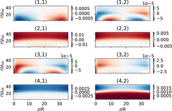
 ⟨NiDKpj⟩t,ϑ
 (PDK,JDK,PGK,JGK)=(6,3,6,5)
 p=1−4
 j=1,2
 p
 z=Lz/2
 p
 z=Lz/2

 NiGKpj
 ⟨NiGKpj⟩t,ϑ
 (PDK,JDK,PGK,JGK)=(6,3,6,5)
 p=1−4
 j=1,2
 p
 z=Lz/2
 p
 z=Lz/2
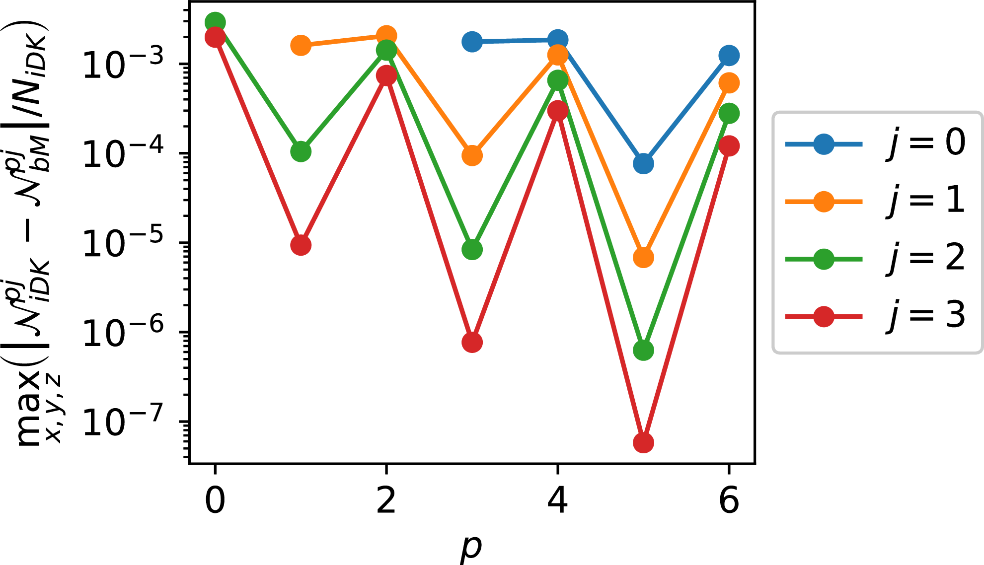
 (PDK,JDK,PGK,JGK)=(6,3,6,5)

 ϕDK
 z=Lz/2
 (PDK,JDK,PGK,JGK)
 PDK=PGK
 JGK=5
 (PDK,JDK)=(2,1)
 ϕDK

 (x,y)
 NDK
 TeDK
 J∥
 ϕDK
 Ω
 U∥
 (PDK,JDK,PGK,JGK)=(6,3,6,5)
 z=Lz/2
 r∼rs∼20ρs0

 (PDK,JDK)=(6,3)

 (z,y)
 NDK
 TeDK
 J∥
 ϕDK
 Ω
 U∥
 (PDK,JDK,PGK,JGK)=(6,3,6,5)
 x=0
 z
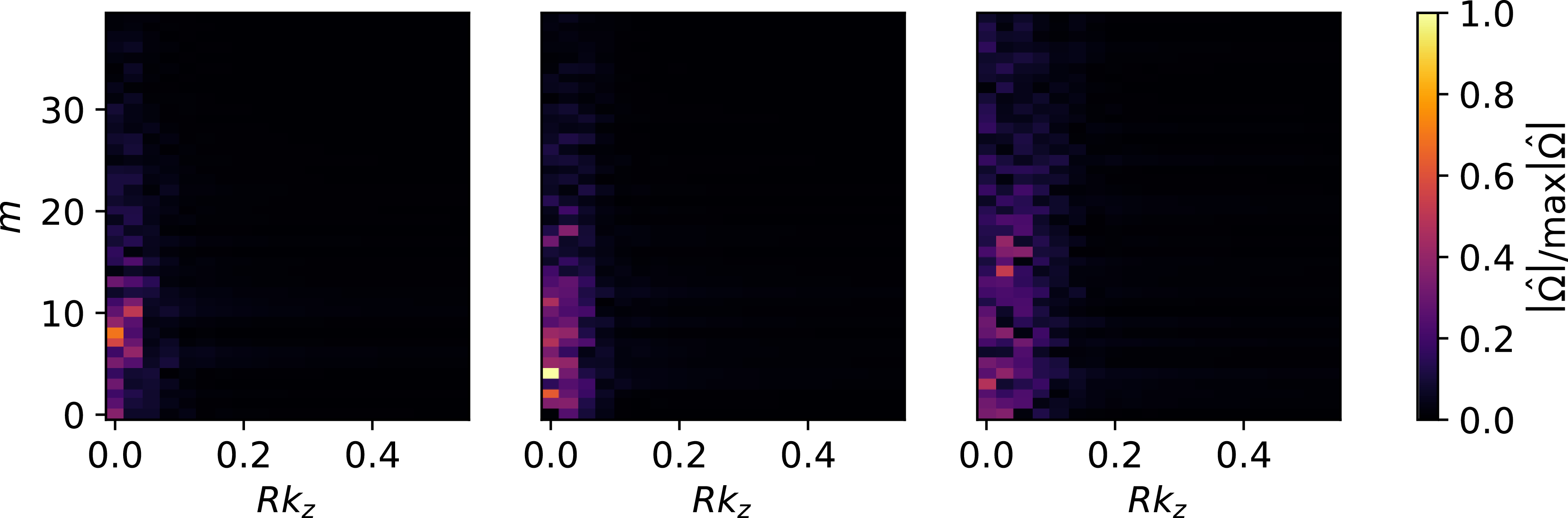
 Ω=∑m,kzΩ^ei(mϑ+kzz)
 r=x2+y2=20ρs0
 (PDK,JDK,PGK,JGK)=(6,3,6,5)
 (PDK,JDK)=(6,3)
 νi0
 1000
 AE
 AN
 10
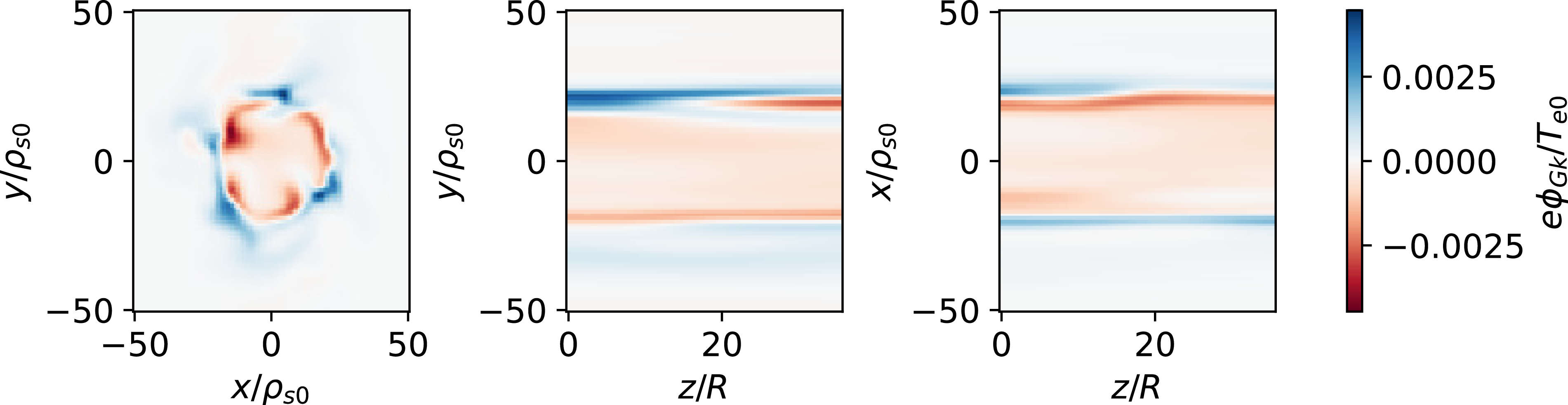
 ϕGK
 z=Lz/2
 x=0
 y=0
 (PDK,JDK,PGK,JGK)=(6,3,6,5)
 ϕGK
 z

 ϕGK
 (kx,ky,z)
 z=0
 kx=0
 ky=0
 (PDK,JDK,PGK,JGK)=(6,3,6,5)
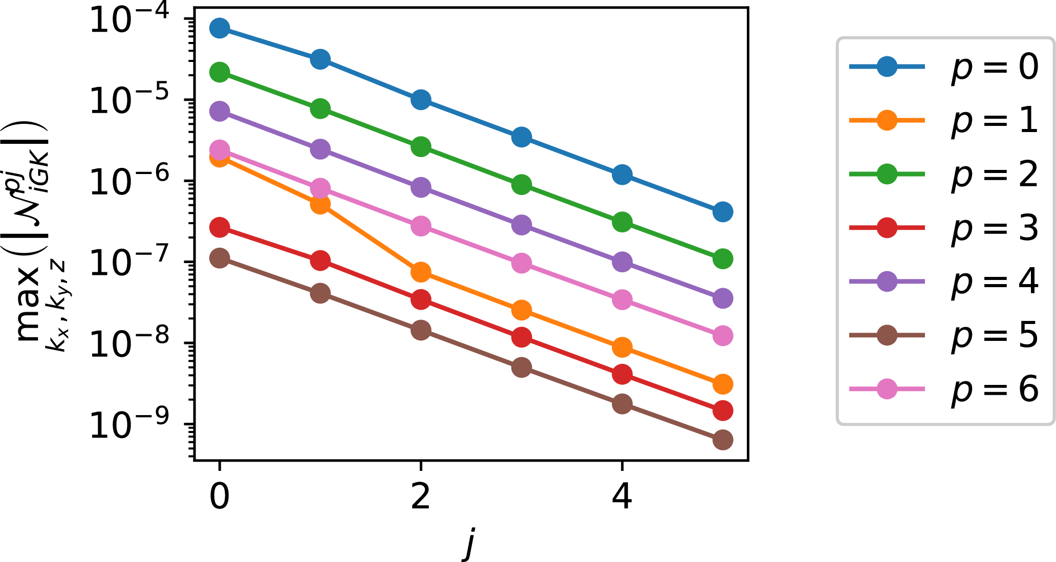
 maxkx,ky,z(|NiGKpj|)
 (PDK,JDK,PGK,JGK)=(6,3,6,5)
 p
 j
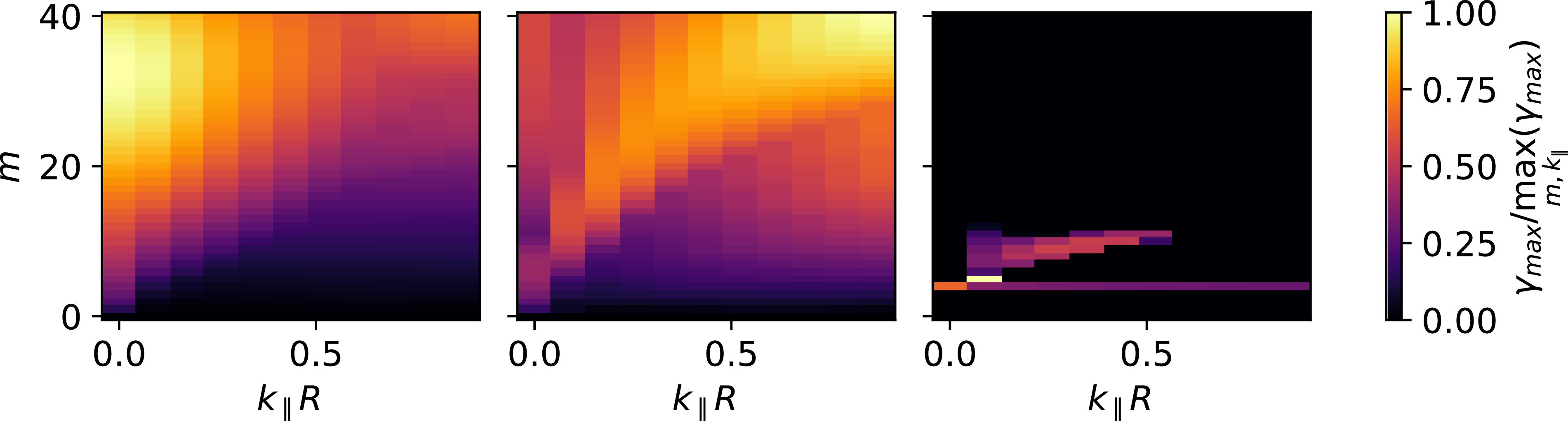
 (PDK,JDK,PGK,JGK)=(4,2,4,3)
 fGK=0
 f~DK=0
 rg=22ρs0
 νi0
 1000
 AE
 AN
 10
 maxm,k∥(γmax)=1.62cs0/R
 maxm,k∥(γmax)=0.91cs0/R
 maxm,k∥(γmax)=0.014cs0/R
 m=33
 k∥=0

 Open access

