The Valence Politics Model of Electoral Choice

Donald Stokes introduced the term valence in a path-breaking article published 50 years ago (Stokes Reference Stokes1963; see also Stokes Reference Stokes1992), which was designed as a critique of the then emerging literature on spatial models of party competition (Downs Reference Downs1957; Black Reference Black1958). Stokes argued that voters rely heavily on their evaluations of rival parties’ perceived capacities to deliver good policy performance in issue areas where there is broad consensus about what government should do. In the language of spatial models, valence issues are ones with very widely shared “ideal points.” A canonical example is the economy. Virtually everyone wants vigorous, sustainable economic growth coupled with low rates of unemployment and inflation. Similarly, almost everyone wants affordable, accessible and effective public services in areas such as education, health, transportation and environmental protection. Vast majorities also demand protection from threats to national and personal security posed by rogue regimes, terrorists and common criminals. Persistent public concern with these valence issues means that they typically dominate the political agenda in Britain and other mature democracies. Valence issues are important in emerging democracies as well (Ho et al. Reference Ho, Clarke, Chen and Weng2013). Although the ordering of specific valence issues on the political agenda varies over time, their persistent salience works to focus debate on “who can do the job” rather than on “what the job should be.” As a consequence, evaluations of which party and which leader are best able to deliver on consensually agreed-upon policy goals are key drivers of voting in most elections and strongly influence party support in inter-election periods.

The major alternative theoretical account of electoral choice—the one which Stokes criticized—is the spatial model of party competition. As its inception, the spatial model has been developed as a formal theory and it also has been subjected to extensive empirical testing (see, e.g., Merrill and Grofman Reference Merrill and Grofman1999; Adams, Merrill and Grofman Reference Adams, Merrill III and Grofman2005). The spatial model’s key assumption is that position or spatial issues are the dominant factors governing voting decisions. Ideal points are not widely shared; indeed, there is considerable disagreement among voters and political leaders over policy goals. See, e.g., the Conservatives differ from Labour on the desirability of cutting taxes as a goal of government policy. Similarly, although both Labour and the Conservatives supported the invasion of Iraq, the Liberal Democrats strongly opposed it, reflecting widespread public disagreement about British involvement in that conflict.

Spatial theory inherited the assumption that voters have exogenously determined issue preferences from neo-classical economic theory. In fact, experimental evidence shows that this assumption is a poor representation of reality (Sanders et al. Reference Sanders, Clarke, Stewart and Whiteley2008), but it nonetheless anchors the theory as individuals attempt to “maximize utility” by supporting a party closest to them in a policy space defined by a general issue-based “left-right” ideological orientation. For their part, parties are strategic actors who try to maximize electoral support in light of knowledge of voter distributions in the commonly shared issue/ideological space. Although spatial models have been imaginatively elaborated in various ways, they retain the core assumption that salient position issues drive the choices of utility-maximizing voters.

With the notable exception of the literature on “economic voting” (e.g., Lewis-Beck Reference Lewis-Beck1988; Duch and Stevenson Reference Duch and Stevenson2008), considerably less attention has been accorded to valence issues compared with spatial ones—despite abundant evidence of the central role that they play in general elections in Britain and elsewhere. Repeated empirical analyses in diverse political milieus demonstrate that valence issues dominate explanations of electoral choice, with spatial issues playing statistically significant but secondary roles (e.g., Clarke et al. Reference Clarke, Sanders, Stewart and Whiteley2004; Clarke et al. Reference Clarke, Sanders, Stewart and Whiteley2009; Clarke, Kornberg and Scotto Reference Clarke, Kornberg and Scotto2009; Clarke and Whitten Reference Clarke and Whitten2013; Ho et al. Reference Ho, Clarke, Chen and Weng2013; Whiteley et al. Reference Whiteley, Clarke, Sanders and Stewart2013). As indicated above, there are good theoretical reasons why this is the case. The costs of information processing are lower for valence compared with spatial issues, and the former are less subject to manipulation than are the latter. Valence-minded voters can rely heavily on readily available heuristics and easily acquired information about existing states of affairs rather than unfulfilled promises and untested policy programs offered by self-serving politicians (see Clarke et al. Reference Clarke, Sanders, Stewart and Whiteley2009, 30–52).

As developed in our studies, the valence model has three key variables that drive voting behavior and party support between elections: evaluations of party performance on valence issues, partisanship and leader images. Valence issues are at the core of the model. A major valence issue, the economy, often dominates electoral politics, although the quality of public services in areas such as health, education and crime prevention can be important too. A strong performance in delivering a prosperous economy, high-quality public services and public safety produces electoral rewards for incumbent parties, whereas a weak performance runs substantial electoral risks.

Leader images and partisan attachments act primarily as heuristic devices in this analysis. In contexts where voters have few incentives to invest time and effort in learning the details of politics and policy making and recognize their limitations in gathering and processing relevant information, they will use cognitive and affective shortcuts to make decisions. Psychologists and experimental economists have stressed the centrality of heuristics (e.g., Kahneman, Slovic and Tversky Reference Kahneman, Slovic and Tversky1982; Gilovich, Griffin and Kahneman Reference Gilovich, Griffin and Kahneman2002; Gigerenzer Reference Gigerenzer2008; Gigerenzer, Hertwig and Pashur Reference Gigerenzer, Hertwig and Pachur2011; Kahneman Reference Kahneman2011; Lupia 1994) and political scientists have recognized their importance for making choices in elections and referendums (Popkin Reference Popkin1991; Sniderman, Brody and Tetlock Reference Sniderman, Brody and Tetlock1991; Lupia and McCubbins Reference Lupia and McCubbins1998; Lupia, McCubbins and Popkin Reference Lupia, McCubbins and Popkin2000). Although heuristics traditionally have been seen as inferior to classical expected utility theory, which underpins the spatial model, research by Gigerenzer (Reference Gigerenzer2008) and Gigerenzer, Hertwig and Pashur (Reference Gigerenzer, Hertwig and Pachur2011) demonstrate that “fast and frugal” heuristics actually are superior to expected utility theory in many “real-world” decision-making situations. This is because the classical model is excessively costly, too slow and in many cases involves intractable calculations, which prevent effective choice. Thus, it does not surprise that straightforward and readily available heuristics involving answers to questions like: “What party do I identify with?,” “Has the economy been getting better or worse?” and “Do I like this particular leader?,” play key roles in explaining why people vote the way they do. If voting involved the kinds of knowledge and calculation required by all but the simplest spatial models then very few people would, or could, do it (see, e.g., Conlisk Reference Conlisk1996). We turn next to specific points raised by EC.

A “Neo-Nuffield” Critique

EC’s central argument is that partisanship is autonomous or exogenous in relation to the other variables that might influence voting and powerfully influences those variables. This is not a new idea as the “Michigan model” developed by the authors of The Voter Decides and The American Voter over half a century ago (Campbell, Gurin and Miller Reference Campbell, Gurin and Miller1954; Campbell et al. Reference Campbell, Converse, Miller and Stokes1960) forcefully asserted that partisanship is a directionally stable long-term force, which influences other important variables in voting models.Footnote ² EC cite recent literature suggesting that partisanship influences issue perceptions, evaluations of leaders and a variety of other variables. We find these claims entirely convincing, but none of them demonstrate that partisanship is directionally stable and exogenous to the other explanatory variables. In the classic “Michigan” analysis, partisanship is typically the product of socialization processes in the family and community, processes arising from experiences in childhood and early adulthood. Once formed it is thought to be directionally stable, except in rare periods of “realignment” caused by major economic and socio-political upheavals. For this reason, partisanship could be reliably characterized as a directionally “unmoved mover”—an autonomous anchor in the skein of forces affecting electoral choice.Footnote ³

When the Michigan model was first introduced into Britain by Butler and Stokes (Reference Butler and Stokes1969) in their seminal book Political Choice in Britain, the central claim was that partisanship in the United Kingdom was strongly rooted in social class. As a person’s class location changes very slowly if at all, the implication is that partisanship exerts a durable and powerful exogenous force on electoral choice. The core argument was summarized with rhetorical flourish by Peter Pulzer (Reference Pulzer1967) in his often-quoted phrase: “in British party politics, class is everything, all else is embellishment and detail.” The class environment in which people were socialized created and subsequently reinforced their partisan attachments which, in turn, did much to explain how they vote. Although there were some exceptions, working-class people largely identified with and voted Labour, whereas middle- and upper-class people identified with and voted Conservative. Minor parties such as the Liberals were not accommodated in this theoretical scheme because, circa the mid-20th century, they had a small and apparently declining vote share. The Liberals and other minor parties were seen as inconsequential curiosities—eccentric relics of Britain’s fading political past.

The problem with this analysis is that it is seriously inconsistent with data from successive British Election Study (BES) panel surveys, including data collected by Butler and Stokes themselves in the 1960s. These data reveal substantial directional instability in partisanship over time. The magnitude of this instability is too great to be explained by migration patterns or the natural turnover of the electorate in periods between adjacent general elections.Footnote ⁴

Data on levels of directional partisan instabilityFootnote ⁵ in several BES multi-wave panel surveys conducted between 1963 and 2006 illustrate the point. The dynamics are consistently impressive—between 29 percent and 38 percent of the respondents report changing their partisan attachments across multiple waves of interviewing (Clarke and McCutcheon Reference Clarke and McCutcheon2009: figure 1). Some people move between parties one or more times, whereas others traverse between partisanship and non-partisanship.Footnote ⁶ Overall, the percentage of BES panelists with stable partisan attachments is somewhat greater in the 1960s than later, but even in the Butler-Stokes era nearly 40 percent failed to exhibit stable partisan attachments. The Michigan model, with its emphasis on directionally stable partisanship, is clearly inconsistent with this evidence.

Reacting to reports of large-scale partisan instability in panel surveys, critics anxious to salvage the conventional Michigan wisdom argued that these analyses were misleading because they failed to take account of random measurement error in survey responses (e.g., Green, Palmquist and Schickler Reference Green, Palmquist and Schickler2002). However, as shown in our previous work (Clarke et al. Reference Clarke, Sanders, Stewart and Whiteley2004; Clarke and McCutcheon Reference Clarke and McCutcheon2009), Mixed Markov Latent Class (MMLC) models (van de Pol and Lengeheine Reference van de Pol and Langeheine1990; Hagenaars and McCutcheon Reference Hagenaars and McCutcheon2002), which take into account such measurement error, consistently reveal that generalized “mover-stayer” models outperform “all stayer” models in BES multi-wave panel surveys conducted since the 1960s).Footnote ⁷ “Mover” groups—those who change their partisan attachments in the MMLC analyses—are always substantial and quite similar in magnitude over time, ranging from a low of 29 percent between 1998 and 2001 and a high of 37 percent between 1992 and 1996 (Clarke and McCutcheon Reference Clarke and McCutcheon2009: figure 5). Over the entire 1963–2006 period, the average size of the mover group in seven four-wave panels is 32 percent. Partisanship in Britain clearly is not the “unmoved mover” of Michigan lore.

There is, of course, a rival theoretical account of partisanship introduced by Fiorina (Reference Fiorina1981); see also Franklin and Jackson (Reference Franklin and Jackson1983), Achen (Reference Achen1992), Franklin (Reference Franklin1992), and Clarke, Stewart and Whiteley (Reference Clarke, Stewart and Whiteley1998), which argues that it is a “running tally” of present and past party performance evaluations with prior evaluations being progressively discounted in favor of more recent ones. As valence issues typically dominate the political agenda, partisanship is largely a weighted sum of over-time judgments about how parties have handled, or would handle, these issues. If a party does badly in delivering on valence issues its brand will be tarnished and its partisan base will erode, whereas a good performance will have the opposite effect of reinforcing the brand and building support. This idea is much more consistent with the evidence on partisan instability than the Michigan model. In the valence politics model partisanship and party performance judgments influence each other over time, and they are part of a larger dynamic system of information processing, which voters use to make political choices. Key variables in the system are mutually endogenous and feed off each other over time. If the underlying theory suggests that interactive dynamics of this kind are what matter, then searching for a mysterious master explanatory variable which is strongly exogenous to all others is a futile exercise.

What does this mean for EC’s critique? There are several noteworthy points. The first is that, if they are correct and partisanship is indeed strongly exogenous to other variables in voting models, then it raises the question as to where do its dynamics come from? One cannot appeal to the Michigan model to solve this conundrum for reasons set out earlier. Partisanship is not only currently unstable at the individual level, but it has been unstable at least since Don Stokes first sampled the Nuffield claret. Similarly, EC themselves rule out the “running tally” model arguing that it is “untenable as perceptions of past performance are themselves shaped by pre-existing partisan affiliations” (p. 6), so that cannot provide a theoretical account. This means that the variable which is thought to anchor the analysis because it is a strongly exogenous determinant of the other variables has no plausible theoretical grounding. Partisanship has large-scale dynamics but where these come from is a mystery, since EC do not account for this “moving mover.”

A second point to make about EC’s critique is methodological. Causality tests should involve all the variables in the valence model with the measures we employ in our analyses: partisanship, evaluations of party performance on key valence issues, leader images and voting intentions, not just two of them which the theory suggests are likely to be strongly correlated in any case. EC do not measure relevant variables the way we do and they neglect to include all of them in their analyses. The implication of valence politics theory as set out above is that one needs to estimate a system, not just selected bivariate relationships. Like all Granger causality tests (Granger Reference Granger1969), the ones EC perform are model dependent (e.g., Enders Reference Enders2010, Chapter 5) and should not be conducted between two variables with a single lag, if they form part of a wider system of interacting relationships with possibly more complex, multiple-lagged dynamics.

A third point concerns EC’s dismissal of contemporaneous or cross-sectional individual-level regressions to estimate effects. In introductory research methods classes, political science graduate students are taught that statistical biases occur in the estimation of models where the left-hand- and right-hand-side variables influence other contemporaneously.Footnote ⁸ The use of lagged predictors and panel data may help to deal with this problem, but not if the actual lags resulting from the theoretical process are very different from the lags used to estimate models. Suppose, e.g., that there is an interactive relationship between voting and partisanship, with both variables having a very rapid impact on each other over time. This will produce biases in a contemporaneous regression where voting is a function of partisanship or partisanship is a function of voting. However, the correct estimates will not be recovered using a panel analysis if the panel waves are far apart, say a year or more, which is typical for BES and other panel surveys. Rather, the coefficients in analysis using such panel data will reflect (possibly many) successive interactions between the two variables over the period between the panel waves with no guarantee that they will capture the true effects.

It is important to note that the number of waves and the intervals between them in BES and other national inter-election panel surveys have been imposed by the practicalities of data collection and research-funding constraints. Lags between adjacent waves of these panel surveys do not necessarily accord with—indeed, may have nothing to do with—the dynamics of voter decision making. The problem will be compounded if there is heterogeneity in these decision-making processes. Some voters may switch their partisan attachments quite frequently depending on the performance of political leaders and the issues of the day, whereas others remain stable, not necessarily because they are strong partisans but because they do not pay much attention to politics. For these reasons, aggregate analyses of closely spaced time series observations in which individual idiosyncrasies are averaged out is likely to provide a more accurate picture of dynamics than do individual-level analyses.

Another important point is that reliable estimates can be obtained from contemporaneous regressions as long as the key predictors are weakly exogenous. If variable y is thought to be explained by variable x, then x is said to be weakly exogenous to y if current values of y do not explain x. Note that unbiased estimation does not require that past values of y do not explain x, which is the definition of strong exogeneity or Granger non-causality (Charezma and Deadman Reference Charezma and Deadman1997). All that is required is that there is no immediate (time t) feedback from y to x. In a dynamic setting of the type that characterizes voter decision making, this means that if variable x has a rapid impact on y, whereas y has a rather slow impact on x, then x can assumed to be weakly exogenous and inferences are valid. Moreover, weak exogeneity is not simply a matter of assumption, as it can be tested empirically if one is confident in the specification of the models that are hypothesized to include the weakly exogenous variables (Charezma and Deadman Reference Charezma and Deadman1997).Footnote ⁹ However, if these models are contested or problematic, attempts to demonstrate weak exogeneity will prove unconvincing.

Regarding weak exogeneity, EC’s structural equation model (EC, figure 2) does not include contemporaneous (time t) causal paths between the latent variables for party performance and party preference. Given that waves of the panel survey are fully one to two years apart, EC are inviting readers to accept the assumption that there is no influence of party performance on party preference or vice versa within one- to two-year time spans. Intuition and analyses of monthly time series data gathered during the New Labour and Thatcher eras suggest that this assumption is implausible (see, e.g., Clarke, Stewart and Whiteley Reference Clarke, Stewart and Whiteley1998; Clarke, Ho and Stewart Reference Clarke, Ho and Stewart2000). If time t effects exist, the model is misspecified, parameter estimates of t−1 effects are biased and, hence, results of Granger causality tests, i.e., the statistical significance of lagged effects (EC, p. 15), are suspect. Again, referring to data gathered one to two years earlier as t−1 may be quite misleading. In terms of the frequency with which voters update information, the variables EC label as t−1 might be t−4, or t−12, or t−52, or …? There is no reason for calling the lag t−1 other than to label the adjacent time point in a panel survey data set available for secondary analysis.

Another difficulty—if time t party performance is not weakly exogenous to time t party preference or vice versa—there will be simultaneity bias. The bias may be trivial, it may be large—who knows? Simply including time t relationships running both ways between party performance and party preference will not do. Inserting these linkages in EC’s model will yield a revised model that violates rank and order conditions for identification at the latent variable level (Bollen Reference Bollen1989; Bollen and Davis Reference Bollen and Davis2009). Instrumental variables will be required for valid inference.

There is yet another problem with EC’s model. They omit cross-lagged linkages between party performance and party preference for 2006–2008 waves of data. However, if they believe that cross-lagged effects obtain for the 2008–2009 and 2009–2010 waves, their omission of such effects for 2006–2008 is theoretically unwarranted. The more general point is that analysts cannot omit what may be important causal linkages and expect remaining coefficients in their models to be unaffected. If empirical warrant for these omissions cannot be supplied, skeptics will label them “incredible” (Sims Reference Sims1980).

The latter point raises additional methodological issues. As the earlier discussion indicates, if hypothesized dependent and independent variables affect each simultaneously, the result is biased parameter estimates. Economists faced the problem of estimating large-scale macro-economic models a generation ago (Fair Reference Fair2004). These “Cowles Commission” models were complex, involving large numbers of simultaneous equations with a great many parameters (Greene Reference Greene2003, 587). However, these models proved inadequate to the task of capturing economic dynamics and accurately forecasting quantities of interest, in part, because analysts had to make arbitrary and unrealistic assumptions about some parameters in order to identify others, so that effects could be empirically estimated.

At the start of the 1980s, the econometrician Christopher Sims (Reference Sims1980) voiced an influential critique of this traditional simultaneous-equation approach to modeling the macro-economy. After delineating the shortcomings of the Cowles Commission approach, Sims introduced his vector autoregressive (VAR) strategy as a way forward. The VAR approach starts with a set of theoretically interesting variables, but avoids making unrealistic assumptions about causal relationships among them (Enders Reference Enders2010; see also Juselius Reference Juselius2006). Rather, the focus is on capturing dynamic relationships among these variables in a series of autoregressive equations. Although promising, a limitation in early work on VAR modeling with mean non-stationary variables was that the models were only able to estimate short-term dynamics and did not incorporate theoretically interesting long-term relationships.Footnote ¹⁰ However, subsequent work on cointegrated relationships has remedied this problem (Engle and Granger Reference Engle and Granger1987; Johansen Reference Johansen1991; Johansen 1996; Juselius Reference Juselius2006). Cointegrated variables are in dynamic long-run equilibrium with each other and it is possible to estimate these relationships at the same time as short-term dynamics are assessed. In the next section, we investigate relationships among key variables in the valence model using a vector error correction model (VECM), which enables us to study the inter-relationships we have been discussing.

A VECM of Governing Party Support in the New Labour Era

As discussed above, the VAR approach is a sensible way of studying inter-relationships among key variables in the valence politics model, given their many possible dynamic inter-relationships. However, traditional BES panel data are inadequate for the purposes of VAR modeling. VAR requires abundant time series observations and, for reasons articulated above, it is desirable to have these data spaced as closely together in time as possible. Here, we employ a time series data set using monthly data gathered over virtually the entire New Labour Era from July 1997 to April 2010 (154 months).Footnote ¹¹ We analyze governing (Labour) party support, as measured by vote intentions over this lengthy period focusing on the effects of key explanatory variables in the valence politics model. These variables include standard measures of partisanship, approval of the job the prime minister is doing and judgments of Labour’s performance on the economy. This large New Labour time series data set provides a useful basis for assessing the valence politics model. If the valence politics model cannot account for the dynamics of governing party support over this extended period, which witnessed prolonged economic good times followed by a deep, protracted recession, then critics such as EC can rightly voice skepticism.

The dynamics of Labour vote intentions, Labour partisanship, prime ministerial approval and Labour performance judgments on the economy are displayed in Figure 1. As shown, all four series decline precipitously over time, with Labour vote intentions falling by 28 points—from 58 percent in July 1997 to 30 percent in April 2010. Partisanship, prime ministerial approval and Labour performance evaluations also decrease substantially, by 20 percent in the case of partisanship, and by 40 percent and 31 percent, respectively, in the cases of prime ministerial approval and judgments about Labour performance on the economy. The numbers for Labour partisanship illustrate the point that partisan attachments in Britain have sizable aggregate- as well as individual-level dynamics. Figure 1 shows that the dynamics of the four valence politics variables are closely inter-related—their average contemporaneous inter-correlation is fully +0.90 (ranging from +0.84 to +0.95).

Fig. 1

Dynamics of Labour vote intentions, prime ministerial approval, Labour performance on economy and Labour partisanship in the New Labour Era, July 1997–April 2010 Note: range of inter-item correlations (time t): r=+0.844 to +0.948. PM=prime ministerial.

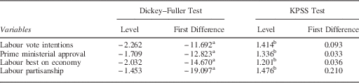
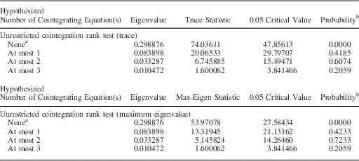
The powerful downward dynamics displayed in Figure 1 testify that the four valence politics variables are mean non-stationary, i.e., they all trend (downwards) over time. This conclusion is confirmed by Dickey–Fuller and KPSS unit root tests (Dickey and Fuller Reference Dickey and Fuller1979; Kwiatkowski et al. Reference Kwiatkowski, Phillips, Schmidt and Shin1992). As Table 1 indicates the four variables are non-stationary in their original level form, but become stationary when first differenced.Footnote ¹² Of course, evidence that variables are non-stationary does not necessarily mean that they are cointegrated—cointegration must be demonstrated empirically. To test for this, we employ the trace and maximum eigenvalue tests proposed by Johansen (Johansen Reference Johansen1991; Johansen 1996). Results of these tests displayed in Table 2 reveal that the four valence politics variables are indeed cointegrated and, moreover, there is one cointegrating vector. The existence of a single cointegrating vector for the four variables comports well with valence politics theory, implying that they all interact with each other in one dynamic long-term equilibrium relationship. During the New Labour Era, Labour vote intentions traveled in dynamic equilbrium with evaluations of the performance of Prime Ministers Tony Blair and Gordon Brown, assessments of Labour’s management of the economy and Labour partisan strength in the electorate.

Table 1

Unit Root Tests for Valence Politics Variables

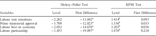
Note: The null hypothesis for the Dickey-Fuller test is that the series is non-stationary; the null hypothesis for the KPSS test is that it is stationary. Dickey–Fuller tests for Labour vote intentions, prime ministerial approval and Labour best on the economy are performed with no lags; tests for Labour party identification performed with one lag.

^a Rejects null hypothesis of non-stationarity, p=0.05, critical value=−2.880.

^b Fails to reject null hypothesis of stationarity, p=0.05, critical value=0.463.

Table 2

Johansen Tests for Cointegrating Relationships Among Labour Vote Intentions, Prime Ministerial Approval, Labour Best on Economy and Labour Party Identification, September 1997–April 2010

Note: Johansen tests performed with three lags for the four variables. Single cointegrating vector also indicated by tests performed with one or two lags. Trace test indicates 1 cointegrating equation(s) at the 0.05 level. Max-eigenvalue test indicates 1 cointegrating equation(s) at the 0.05 level.

^a Denotes rejection of the hypothesis at the 0.05 level.

^b MacKinnon-Haug-Michelis (1999) p-values.

Within the general VAR modeling framework the existence of a cointegrating relationship for these four variables mandates the specification of a VECM to capture their mutual inter-relationships (Juselius Reference Juselius2006). The general VECM is:

$$\Delta X_{t} =\mu {\plus}\Gamma _{1} \Delta X_{{t{\minus}1}} {\plus}\,\,\ldots\,\,\Gamma _{k} \Delta X_{{t{\minus}k}} {\plus}\alpha B'X_{{t{\minus}1}} {\plus}Z_{{t{\minus}p}} {\plus}{\varepsilon}_{t} ,$$

where, X _t is the vector of non-stationary variables with order of integration d; ∆ the differencing operator; Γ_1−k the matrix of parameters for short-run effects of variables, 1 to k lags; α the adjustment parameters for r cointegrating vectors; β′X _t−1=r×1 vector of stationary cointegrating relations; Z _t−p the vector of strongly exogenous variables operating at t−p lags; μ the constant; and ε _t the stochastic error term ~N(0, σ ²).

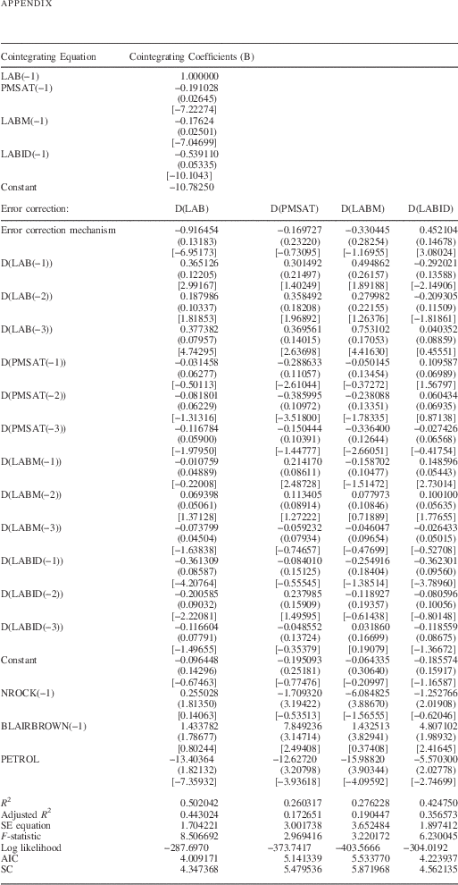
In the present analysis, the VECM system has four equations, one for each variable of interest, i.e., Labour vote intentions, prime ministerial approval, Labour performance on economy and Labour partisanship. In addition to the error correction mechanism implied by the cointegrating relationship among the four variables, diagnostic tests indicate that three lags of first-differenced versions of the variables can be included, each of these four equations to capture short-term effects. Three additional strongly exogenous dummy variables are added to take into account shocks to the system caused by the petrol crisis (September 2000), the replacement of Tony Blair by Gordon Brown as prime minister (June 2007) and the Northern Rock bank crisis (September 2007). Parameter estimates for the VECM (see Appendix) show that the error correction mechanism in the Labour vote intention equation is very strong. The adjustment parameter for the error correction mechanism is −0.92, indicating that slightly over 90 percent of a shock to the system, from whatever source, is eroded in the month following its occurrence. Valence politics considerations clearly dominate the system’s dynamics in the New Labour Era.

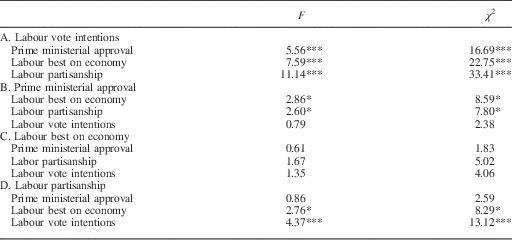
The existence of a very powerful long-run relationship among the four key valence variables implies that Granger causal processes (Granger Reference Granger1969) are at work. As Giles (Reference Giles2011) states: “[i]f two or more time series are cointegrated then there must be Granger causality between them—either one-way or in both directions.” There are nine possibilities when dealing with the four variables in the system, i.e., Labour vote intentions, Labour partisanship, prime ministerial approval and judgments about Labour’s performance on the economy. If valence politics theory is correct, over time these variables should have a variety of influences on each other.Footnote ¹³Table 3 documents that this is the case. Prime ministerial approval, judgments about Labour performance on the economy and Labour partisanship all Granger cause Labour vote intentions. In addition, Labour partisanship and Labour performance on the economy Granger cause prime ministerial approval, and Labour performance on the economy and Labour vote intentions Granger cause Labour partisanship. Only Labour performance on the economy appears to be autonomous vis-à-vis the other three variables.

Table 3

Granger Causality Tests for Labour Vote Intentions, Prime Ministerial Approval, Labour Best on Economy and Labour Partisanship

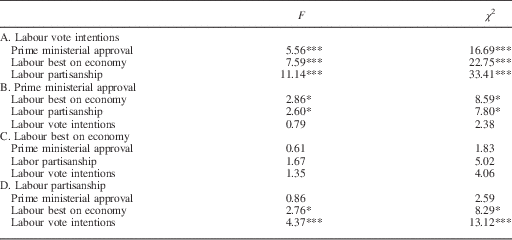
Note: block exogeneity tests using VAR in levels; three lags for each tested predictor and four lags for non-tested predictors.

VAR=vector autoregressive.

Rejects null hypothesis of Granger non-causality; *p<0.05; **p<0.01; ***p<0.001.

Another perspective on the flow of influence in the VECM system is provided by converting it to a moving average representation (MAR) and assessing the impact of shocks to one variable on the other variables. Using the conventional Cholesky decomposition for an impulse response analysis requires the analyst to order the variables according to a hypothesized flow of influence in the system, and so results are potentially sensitive to alternative orderings (see Enders Reference Enders2010, Chapter 5). In the present case, the flow of influence in the system is a major point at issue. Accordingly, we employ the generalized impulse response analysis methodology developed by Pesaran and Shin (Reference Pesaran and Shin1998). Results of this approach are invariant to variable orderings in the VAR or VECM.

The results for the valence politics VECM are displayed in the four panels in Figure 2. As the figure shows, one standard deviation shocks to any of the four variables in the system have a variety of immediate- and lagged effects on the other three variables. Of particular interest, the upper left-hand panel shows that Labour vote intentions respond quite strongly to shocks to Labour performance on the economy, Labour partisanship and prime ministerial approval. Ceteris paribus, after three months, Labour vote intentions would increase by from approximately 0.72 to 1.52 SD, as a result of shocks to other variables in the system, with the effects of judgments about Labour’s performance on the economy being the strongest and Labour partisanship the weakest.

Fig. 2

Generalized impulse response functions over six time periods for vector error correction (VEC) model of relationships among Labour vote intentions, prime ministerial approval, Labour best on the economy and Labour party identification, September 1997–April 2010 Note: PM=prime ministerial; Id=identification.

The cumulative effects of shocks to variables in the system are shown in Figure 3. As one would expect, given the powerful cointegrating relationship among vote intentions and the other three variables and evidence of Granger causal effects, all of these cumulative effects on Labour vote intentions should be very substantial. Although the Ceteris paribus assumptions underlying the scenario on Figure 3 are unlikely to obtain in practice, as negative shocks often quickly work to counteract positive ones, the potential power of valence politics considerations is clearly evident. The MAR analysis summarized in Figures 2 and 3 show a wide variety of strong responses across the VECM for the valence politics variables. This is exactly what one would expect if these variables constitute the strongly interactive, dynamic system, predicted by valence theory.

Fig. 3

Accumulated generalized impulse responses in Labour vote intentions over six time periods for vector error correction (VEC) model of relationships among Labour vote intentions, prime ministerial approval, Labour best on economy and Labour party identification, September 1997–April 2010 Note: PM=prime ministerial; Id=identification.

Conclusion: A Plea to Stop Hunting Snarks

In their critique, EC propose a model which they label “the valence politics model of electoral choice.” This model is a curious beast, one we do not recognize as the dependent variable is something called “Labour preference,” which does not appear either conceptually or operationally in our work, except as occasional stylistic relief for “vote choice” or “vote intentions.”Footnote ¹⁴ In addition, key explanatory variables in our valence politics model are missing (e.g., leader images, party best on most important issue) or measured in ways different from what we do (e.g., partisanship). Given these several modifications to the valence politics model, it does not surprise that EC’s model performs differently than the one used in our analyses. When we “round up the usual suspects,” use our standard conceptual and operational definitions of variables of interest, and employ appropriate methods for investigating EC’s claim that partisanship is strongly exogenous, the results strongly support our version of valence politics model. Partisanship is not strongly exogenous in this system; rather it interacts in various ways with other key valence politics variables including party performance judgments, prime ministerial approval and the vote itself.

Model specification, variable measurement and statistical methods are very important issues to be sure; however, in a sense they are ultimately secondary considerations. The fundamental problem with EC’s critique is their subtle, yet seductive, invitation to seek a magic variable that could account for the observed dynamics in voting, leader images and party performance judgments. EC believe that the variable is partisanship which, by their account, drives all the other variables under consideration. However, if EC are right, then partisanship must itself exhibit dynamic properties. After all, voting behavior, images of party leaders and evaluations of parties’ ability to deal with major issues such as the economy clearly manifest large-scale movements and one cannot explain variation with a constant. Of course, partisanship does move, both at the aggregate- and individual levels in Britain. As observed above, partisan flexibility is not novel; rather it has been a feature of British political psychology since at least the early 1960s, when Stokes first accepted Butler’s invitation to temporarily decamp chilly Ann Arbor and bring his theoretical ideas and survey methodology to welcoming Nuffield.

However, what moves partisanship? It is here that EC invite readers to begin the search. In an earlier time, Butler and Stokes and others at Nuffield had conjectured that social class was the magic variable. However, class clearly did not exhibit the behavior required to explain either the sizable dynamics observed in the BES panel surveys or the large-scale change witnessed in successive general elections. However, if social class is not the magic variable that moves all other movers, then what is?

As argued above, we believe accepting an invitation to search for a magic variable is ultimately a fruitless task. For well over half a century, EC and other students of voting behavior in Britain, the United States and elsewhere have employed data from periodic national election studies to try to find this fabled “snark.” Provocative and intriguingly counter-intuitive, EC’s critique illustrates the kind of analysis that perpetuates theoretical and methodological problems that beset the field of electoral studies. In particular, their critique nicely illustrates the limitations of traditional election study data-gathering methods. Reluctant or unable to break free from the survey research techniques pioneered in Ann Arbor nearly 70 years ago, many political scientists do not conduct the very high frequency, very large N, panel surveys that would provide needed leverage for studying the kinds of tightly inter-related dynamic systems of beliefs, attitudes and behavior that drive individual and collective electoral choice and other forms of citizen political action.Footnote ¹⁵ Whatever virtues traditional election surveys may have, they cannot do the methodological job demanded of them when asked to help answer important, longstanding theoretical questions such as those discussed above. Hugely expensive, low frequency, small N, face-to-face “convenience samples in time,” these surveys were leading-edge methodology, when the Beatles were playing the Cavern in Liverpool and Stokes was enjoying the conviviality of the Nuffield high table. That moment is now long past and conventional election surveys are not the “big Hadron colliders” needed to advance electoral inquiry in the 21st century.Footnote ¹⁶ Like their colleagues in the natural sciences, electoral researchers need to design and implement the data-gathering instruments required to answer central theoretical questions.

A final point about theory, we say again (more than three times!) there are no snarks—no magic hidden variables, the powerful effects of which will be revealed by just one more regression/logit/probit/SEM analysis of traditional survey data from just one more new election study. The variables in the valence politics model presented above do not explain everything about electoral choice, but they provide powerful theoretical and empirical insights into what is going on in the minds of voters. Supplemented by selected variables from spatial theory, the result is a parsimonious composite modelFootnote ¹⁷ that goes a long way toward providing a satisfactory explanation of voting in Britain and elsewhere. There is no need to rummage around one more time in the dark recesses of the famed “funnel of causality” to find that sly snark. It’s not there.Appendix