1. Introduction
The mathematical formulation of the Richardson–Kolmogorov cascade (Richardson Reference Richardson1922; Kolmogorov Reference Kolmogorov1941a
,Reference Kolmogorov
b
,Reference Kolmogorov
c
; Batchelor Reference Batchelor1953) is based on the evolution equation for the second-order structure function
 $\overline{{\it\delta}q^{2}}=\overline{({\it\delta}u_{i})^{2}}$
(with an implicit summation over the index
 $i$
) where the overbar denotes an average over realisations or, in practice in this paper, over time. In this structure function,
 ${\it\delta}u_{i}\equiv u_{i}-u_{i}^{\prime }$
where
 $u_{i}~(i=1,2,3)$
is a fluctuating velocity component at a location
 $\boldsymbol{x}=\boldsymbol{X}+\boldsymbol{r}/2$
in the turbulent flow and
 $u_{i}^{\prime }$
is the same fluctuating velocity component at a different location, namely
 $\boldsymbol{x}^{\prime }=\boldsymbol{X}-\boldsymbol{r}/2$
. This evolution equation is usually referred to as the Kármán–Howarth or Kármán–Howarth–Monin equation and it can be written down without assumptions of statistical homogeneity and isotropy (see Deissler Reference Deissler1961; Hill Reference Hill2002; Marati, Casciola & Piva Reference Marati, Casciola and Piva2004; Danaila et al.
Reference Danaila, Krawczynski, Thiesset and Renou2012; Valente & Vassilicos Reference Valente and Vassilicos2015), in which case
 $\overline{{\it\delta}q^{2}}$
is a function of both the centroid
 $\boldsymbol{X}$
and the separation vector
 $\boldsymbol{r}$
. The starting point is the Navier–Stokes equation for incompressible flow, where the velocity and pressure fields have been decomposed into mean (in upper case notation) and fluctuating (in lower case notation) fields, i.e.
 $$\begin{eqnarray}\frac{\partial (U_{i}+u_{i})}{\partial t}+(U_{k}+u_{k})\frac{\partial U_{i}+u_{i}}{\partial x_{k}}=-\frac{1}{{\it\rho}}\frac{\partial }{\partial x_{i}}(P+p)+{\it\nu}{\rm\nabla}^{2}(U_{k}+u_{k})\end{eqnarray}$$
(
 ${\it\rho}$
and
 ${\it\nu}$
are respectively the mass density and kinematic viscosity of the fluid). By incompressibility,
 $(\partial /\partial x_{i})U_{i}=(\partial /\partial x_{i})u_{i}=0$
. Using the Navier–Stokes and incompressibility equations at both locations
 $\boldsymbol{x}$
and
 $\boldsymbol{x}^{\prime }$
and operating a change of variables from (
 $\boldsymbol{x},\boldsymbol{x}^{\prime }$
) to (
 $\boldsymbol{X},\boldsymbol{r}$
) one derives the following Kármán–Howarth–Monin equation by standard mathematical manipulations (see Hill Reference Hill2002; Marati et al.
Reference Marati, Casciola and Piva2004; Danaila et al.
Reference Danaila, Krawczynski, Thiesset and Renou2012; Valente & Vassilicos Reference Valente and Vassilicos2015):
 $$\begin{eqnarray}\displaystyle & & \displaystyle \frac{\partial \overline{{\it\delta}q^{2}}}{\partial t}+\left(\frac{U_{k}+U_{k}^{\prime }}{2}\right)\frac{\partial \overline{{\it\delta}q^{2}}}{\partial X_{k}}+\frac{\partial \overline{{\it\delta}u_{k}{\it\delta}q^{2}}}{\partial r_{k}}+\frac{\partial {\it\delta}U_{k}\overline{{\it\delta}q^{2}}}{\partial r_{k}}\nonumber\\ \displaystyle & & \displaystyle \quad =4\mathscr{P}+4\mathscr{T}+4\mathscr{T}_{p}+4\mathscr{D}_{{\it\nu}}+4\mathscr{D}_{X,{\it\nu}}-4{\it\epsilon}^{\ast },\end{eqnarray}$$
where
 ${\it\delta}U_{k}\equiv U_{k}-U_{k}^{\prime }$
,
 ${\it\delta}p\equiv p-p^{\prime }$
and
-
(i)
 $4\mathscr{P}(\boldsymbol{X},\boldsymbol{r})\equiv -2\overline{u_{k}{\it\delta}u_{i}}\partial U_{i}/\partial x_{k}+2\overline{u_{k}^{\prime }{\it\delta}u_{i}}\partial U_{i}^{\prime }/\partial x_{k}^{\prime }$
represents the turbulent production term, which is kept in its expression as a function of
$\boldsymbol{x}=\boldsymbol{X}+\boldsymbol{r}/2$
and
$\boldsymbol{x}^{\prime }=\boldsymbol{X}-\boldsymbol{r}/2$
;
-
(ii)
$4\mathscr{T}(\boldsymbol{X},\boldsymbol{r})\equiv -\partial /\partial X_{k}(\overline{(u_{k}+u_{k}^{\prime }){\it\delta}q^{2}}/2)$
represents turbulent transport along
$\boldsymbol{X}$
of
${\it\delta}q^{2}\equiv ({\it\delta}u_{i})^{2}$
which is a function of
$\boldsymbol{X}$
and
$\boldsymbol{r}$
; -
(iii)
$4\mathscr{T}_{p}(\boldsymbol{X},\boldsymbol{r})\equiv -2/{\it\rho}\partial \overline{{\it\delta}u_{k}{\it\delta}p}/\partial X_{k}$
represents turbulent transport along
$\boldsymbol{X}$
of
${\it\delta}p(\boldsymbol{X},\boldsymbol{r})$
; -
(iv)
$4\mathscr{D}_{{\it\nu}}(\boldsymbol{X},\boldsymbol{r})\equiv 2{\it\nu}\partial ^{2}\overline{{\it\delta}q^{2}}/\partial r_{k}^{2}$
is the viscous diffusion in the space of separation vectors
$\boldsymbol{r}$
(note that
$\mathscr{D}_{{\it\nu}}(\boldsymbol{X},\boldsymbol{r})={\it\epsilon}(\boldsymbol{X})$
in the limit
$|\boldsymbol{r}|\equiv r\rightarrow 0$
); -
(v)
$4\mathscr{D}_{X,{\it\nu}}(\boldsymbol{X},\boldsymbol{r})\equiv {\it\nu}/2\partial ^{2}\overline{{\it\delta}q^{2}}/\partial X_{k}^{2}$
is the viscous diffusion in physical space (i.e. along
$\boldsymbol{X}$
); -
(vi)
$4{\it\epsilon}^{\ast }(\boldsymbol{X},\boldsymbol{r})\equiv 2{\it\nu}\overline{(\partial u_{i}/\partial x_{k})^{2}}+2{\it\nu}\overline{(\partial u_{i}^{\prime }/\partial x_{k}^{\prime })^{2}}$
is the sum of two times the turbulent kinetic energy dissipation evaluated at each location with
${\it\epsilon}^{\ast }=({\it\epsilon}+{\it\epsilon}^{\prime })/2$
.
















By assuming that at small enough separations
 $r\equiv |\boldsymbol{r}|$
the turbulence is locally statistically homogeneous in the frame moving with the mean flow, all the terms on the right-hand side of (1.2) vanish except
 $4\mathscr{D}_{{\it\nu}}$
and
 $4{\it\epsilon}^{\ast }$
. Furthermore, the viscous diffusion term
 $4\mathscr{D}_{{\it\nu}}$
can reasonably be neglected at high enough Reynolds numbers for a given
 $r$
that is larger than length scales where viscous diffusion is significant. With these simplifying assumptions, (1.2) becomes
 $$\begin{eqnarray}\frac{\partial \overline{{\it\delta}q^{2}}}{\partial t}+\left(\frac{U_{k}+U_{k}^{\prime }}{2}\right)\frac{\partial \overline{{\it\delta}q^{2}}}{\partial X_{k}}+\frac{\partial \overline{{\it\delta}u_{k}{\it\delta}q^{2}}}{\partial r_{k}}=-4{\it\epsilon}.\end{eqnarray}$$
The only remaining terms are
-
(i)
$4\mathscr{A}_{t}(\boldsymbol{X},\boldsymbol{r})\equiv \partial \overline{{\it\delta}q^{2}}/\partial t$
(which cancels when the flow is statistically stationary and the average can be taken over time); -
(ii)
$4\mathscr{A}(\boldsymbol{X},\boldsymbol{r})\equiv (U_{k}+U_{k}^{\prime })/2\partial \overline{{\it\delta}q^{2}}/\partial X_{k}$
, which is the advection of
$\overline{{\it\delta}q^{2}}(\boldsymbol{X},\boldsymbol{r})$
by the mean flow (and which equals
$U_{k}\partial \overline{{\it\delta}q^{2}}/\partial X_{k}$
when there is statistical homogeneity); -
(iii)
$4{\it\Pi}(\boldsymbol{X},\boldsymbol{r})\equiv \partial \overline{{\it\delta}u_{k}{\it\delta}q^{2}}/\partial r_{k}$
, which is the nonlinear energy transfer term; the divergence of the flux
$\overline{{\it\delta}u_{k}{\it\delta}q^{2}}$
transfers fluctuating energy from spherical shells centred at
$\boldsymbol{X}$
with radius
$r=|\boldsymbol{r}|$
either to spherical shells centred at the same
$\boldsymbol{X}$
but with different radius or within the same spherical shell but to a different orientation
$\boldsymbol{r}/r$
; -
(iv)
$4{\it\epsilon}^{\ast }(\boldsymbol{X},\boldsymbol{r})\equiv 4({\it\epsilon}+{\it\epsilon}^{\prime })/2$
, which equals
$4{\it\epsilon}$
when there is statistical homogeneity.









It should be noted that statistical homogeneity has also allowed us to discard
 $4{\it\Pi}_{U}(\boldsymbol{X},\boldsymbol{r})=\partial {\it\delta}U_{k}\overline{{\it\delta}q^{2}}/\partial r_{k}$
, which is the linear energy transfer by the mean flow and which has a similar interpretation to
 $4{\it\Pi}(\boldsymbol{X},\boldsymbol{r})$
but in relation to the flux
 $U_{k}\overline{{\it\delta}q^{2}}$
.
The critical equilibrium assumption made by Kolmogorov (Reference Kolmogorov1941a
,Reference Kolmogorov
b
,Reference Kolmogorov
c
) is that, at high enough Reynolds number, the time scales characterising the evolution of
 $\overline{{\it\delta}q^{2}}$
at small enough scales
 $r$
are much smaller than the time scale characterising homogeneous turbulence decay, thus implying
 $$\begin{eqnarray}\frac{\partial \overline{{\it\delta}q^{2}}}{\partial t}+\left(\frac{U_{k}+U_{k}^{\prime }}{2}\right)\frac{\partial \overline{{\it\delta}q^{2}}}{\partial X_{k}}\approx 0.\end{eqnarray}$$
Kolmogorov’s assumption leads directly to an equilibrium between nonlinear energy transfer and dissipation which is the crux of the Richardson–Kolmogorov cascade, namely
 $$\begin{eqnarray}\frac{\partial \overline{{\it\delta}u_{k}{\it\delta}q^{2}}}{\partial r_{k}}\approx -4{\it\epsilon}.\end{eqnarray}$$
Integrating both sides of this balance over a sphere of radius
 $|\boldsymbol{r}|=r$
as in Nie & Tanveer (Reference Nie and Tanveer1999) and making use of the Gauss divergence theorem we obtain
 $$\begin{eqnarray}\int \overline{{\it\delta}\boldsymbol{u}{\it\delta}q^{2}}\boldsymbol{\cdot }\frac{\boldsymbol{r}}{r}\,\text{d}{\it\Omega}\approx \int -4{\it\epsilon}\,\text{d}V=-\frac{16{\rm\pi}}{3}{\it\epsilon}r,\end{eqnarray}$$
where
 $\text{d}{\it\Omega}$
and
 $\text{d}V$
are differentials of a solid angle and a volume respectively. If the assumption of small-scale isotropy is made, i.e. that
 $\overline{{\it\delta}\boldsymbol{u}{\it\delta}q^{2}}\boldsymbol{\cdot }(\boldsymbol{r}/l)$
is independent of the orientation of the unit vector
 $\boldsymbol{r}/r$
, then this integral yields the expression
 $$\begin{eqnarray}\overline{{\it\delta}\boldsymbol{u}_{\Vert }{\it\delta}q^{2}}\approx -{\textstyle \frac{4}{3}}{\it\epsilon}r,\end{eqnarray}$$
where
 ${\it\delta}\boldsymbol{u}_{\Vert }\equiv {\it\delta}\boldsymbol{u}\boldsymbol{\cdot }\boldsymbol{r}/r$
. This expression and the equilibrium balance equation (1.5) are the central properties of the Richardson–Kolmogorov cascade and are valid over the so-called inertial range of scales
 $r$
which are neither too small for viscous effects to be significant nor too large to be comparable with the size of the largest turbulent eddies where Kolmogorov’s assumption (1.4) will certainly break down. The minus sign in (1.7) indicates that the energy cascades from large to small scales, and the independence of the equilibrium balance (1.5) on
 $\boldsymbol{r}$
(as long as
 $r$
is in the inertial range) implies a self-similar cascade, i.e. one where the divergence of the flux
 $\overline{{\it\delta}u_{k}{\it\delta}q^{2}}$
is independent of
 $\boldsymbol{r}$
and proportional to the dissipation rate
 ${\it\epsilon}$
. This last concept then sets the foundations for the dimensional analysis which leads to the celebrated
 $2/3$
and
 $-5/3$
respective scalings of the second-order structure function and the energy spectrum of small-scale turbulence (Kolmogorov Reference Kolmogorov1941a
,Reference Kolmogorov
b
,Reference Kolmogorov
c
; Batchelor Reference Batchelor1953).
In the present paper we explore these ideas in a non-homogeneous turbulence where (1.3) is not valid and one therefore needs to revert to the full non-homogeneous Kármán–Howarth–Monin equation (1.2). However, we explore these ideas in a highly inhomogeneous part of a turbulent flow where Kolmogorov’s
 $2/3$
power law has been reported to exist, namely in the production region of a turbulent flow generated by a fractal square grid obstructing a free stream (Laizet, Vassilicos & Cambon Reference Laizet, Vassilicos and Cambon2013; Gomes-Fernandes, Ganapathisubramani & Vassilicos Reference Gomes-Fernandes, Ganapathisubramani and Vassilicos2014). The production region is a region near the turbulence-generating grid where the turbulence does not decay with streamwise distance at all spanwise locations but in fact grows with streamwise distance, in particular along the centreline where it grows for the longest streamwise extent. The advantage of a fractal square grid over a regular one, for example, is that the fractal square grid magnifies the spatial extent of the production region and abates its activity there, thus making measurements possible or at the very least less difficult, see Mazellier & Vassilicos (Reference Mazellier and Vassilicos2010), Laizet & Vassilicos (Reference Laizet and Vassilicos2011, Reference Laizet and Vassilicos2012, Reference Laizet and Vassilicos2015) and Nagata et al. (Reference Nagata, Sakai, Suzuki, Suzuki, Terashima and Inaba2013) who have documented the inhomogeneous and anisotropic nature of the production region downstream of a fractal grid, and in particular Laizet & Vassilicos (Reference Laizet and Vassilicos2012, Reference Laizet and Vassilicos2015) who have made comparisons with regular grids.
In § 2 we describe our experimental facility and measurement locations and technique and in § 3 we present our first results concerning energy spectra and the third-order structure function
 $\overline{{\it\delta}\boldsymbol{u}_{\Vert }{\it\delta}q^{2}}$
. In § 4 we describe how we reduce from our measurements the different terms in (1.2), what assumptions we make and what terms we are unable to obtain. In §§ 5 and 6 we report on these terms and we conclude in § 7.
2. Experimental details
2.1. Experimental facility and grid geometry details
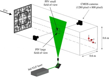
Experiments are carried out in a recirculating water tunnel whose schematic is shown in figure 1. The test section has a cross sectional area of
 $0.6~\text{m}\times 0.6~\text{m}$
and is 9 m long. Transparent perspex sheets are installed as a roof to prevent any gravitational waves from interfering with the flow. The free-stream turbulence intensity is 2.8 % for the streamwise fluctuating velocity
 $u$
and 4.4 % for the spanwise fluctuating velocity
 $v$
. For more details on the experimental facility see Gomes-Fernandes, Ganapathisubramani & Vassilicos (Reference Gomes-Fernandes, Ganapathisubramani and Vassilicos2012) and Gomes-Fernandes et al. (Reference Gomes-Fernandes, Ganapathisubramani and Vassilicos2014).
Schematic of the water tunnel and particle image velocimetry (PIV) set-up.

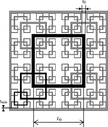
In the present work, the space-filling fractal square grid SFG17 is used. This fractal grid was introduced by Hurst & Vassilicos (Reference Hurst and Vassilicos2007) and then used for turbulence studies by Seoud & Vassilicos (Reference Seoud and Vassilicos2007), Mazellier & Vassilicos (Reference Mazellier and Vassilicos2010), Valente & Vassilicos (Reference Valente and Vassilicos2011), Gomes-Fernandes et al. (Reference Gomes-Fernandes, Ganapathisubramani and Vassilicos2012), Discetti et al. (Reference Discetti, Ziskin, Astarita, Adrian and Prestridge2013), Nagata et al. (Reference Nagata, Sakai, Suzuki, Suzuki, Terashima and Inaba2013), Gomes-Fernandes et al. (Reference Gomes-Fernandes, Ganapathisubramani and Vassilicos2014) and Valente & Vassilicos (Reference Valente and Vassilicos2014). There is therefore a wealth of data by now on the turbulence generated by this grid. Figure 2 shows a schematic of the SFG17. It has four ‘fractal iterations’ (
 $N$
), a thickness ratio (
 $t_{r}$
) of 17 (
 $t_{r}$
is the ratio between the thickness of the thickest bar
 $t_{0}$
and that of the thinnest bar
 $t_{min}$
) and a blockage ratio of 25 %. The length of the thickest bars is
 $L_{0}$
. The ratio between the lengths of two consecutive iterations,
 $R_{L}=L_{i+1}/L_{i}$
(
 $i$
from 0 to
 $N-1$
), is
 $1/2$
. Defined in a similar way, the ratio between the thickness of two consecutive iterations,
 $R_{t}=t_{i+1}/t_{i}$
, is
 $t_{r}^{1/(N-1)}$
. The grid thickness in the streamwise direction is 5 mm. Full geometrical details are found in table 1.
Schematic of the SFG17 after Gomes-Fernandes et al. (Reference Gomes-Fernandes, Ganapathisubramani and Vassilicos2012). The
 $N\,=\,4$
‘fractal iterations’ are highlighted in black, and further details on the geometrical parameters are found in table 1.

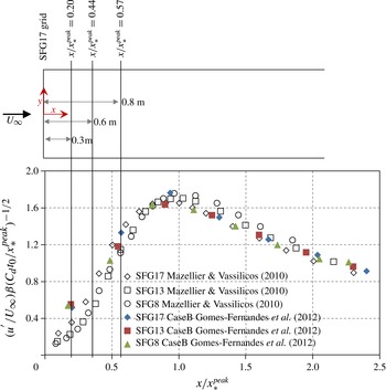
Streamwise evolution of the centreline turbulence intensity generated by space-filling square fractal grids after Gomes-Fernandes et al. (Reference Gomes-Fernandes, Ganapathisubramani and Vassilicos2012, p. 325), and a plan view of the measurement locations for the present study.

Space-filling fractal square grid SFG17 geometric details;
 $t_{min}=t_{3}$
,
 $L_{min}=L_{3}$
.

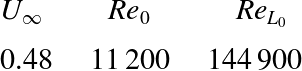
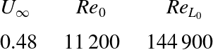
The inlet velocity
 $U_{\infty }$
was set to
 $0.48~\text{m}~\text{s}^{-1}$
, Case A of Gomes-Fernandes et al. (Reference Gomes-Fernandes, Ganapathisubramani and Vassilicos2012). Table 2 shows a summary of the inlet velocities and global Reynolds numbers for the present study. The global Reynolds number is denoted in this way given that it does not depend on space and time as it is fully determined by the inlet conditions.
Experimental conditions: free-stream velocities and global Reynolds numbers. Here,
 $\mathit{Re}_{0}$
and
 $\mathit{Re}_{L_{0}}$
are the Reynolds numbers based on the thickness
 $t_{0}$
and the length
 $L_{0}$
respectively (see figure 2):
 $\mathit{Re}_{0}=U_{\infty }t_{0}/{\it\nu}$
and
 $\mathit{Re}_{L_{0}}=U_{\infty }L_{0}/{\it\nu}$
.
2.2. Measurement locations
Before describing our measurement technique, we need to explain how we chose our measurement locations. Figure 3 shows the behaviour of the turbulence intensity of the streamwise velocity fluctuation (
 $u^{\prime }/U_{\infty }$
) generated by space-filling fractal square grids from two different experiments (Mazellier & Vassilicos Reference Mazellier and Vassilicos2010; Gomes-Fernandes et al.
Reference Gomes-Fernandes, Ganapathisubramani and Vassilicos2012). The streamwise distance
 $x$
is normalised by
 $x_{\ast }^{peak}\propto L_{0}^{2}/({\it\alpha}C_{d}t_{0})$
, where
 ${\it\alpha}$
is a parameter that takes into account the incoming free-stream turbulence and
 $C_{d}$
is the drag coefficient of the thickest bar if assumed to be of infinite length. This scale
 $x_{\ast }^{peak}$
is an estimator of the turbulence intensity peak location and an improvement on the wake interaction length scale introduced by Mazellier & Vassilicos (Reference Mazellier and Vassilicos2010). It should be noted that in the present case
 $x_{\ast }^{peak}=1.36~\text{m}$
, which allows us to have a considerable physical space to perform PIV in the production region, as opposed to what happens with usual regular grids, where
 $x_{\ast }^{peak}\approx 3M$
, with
 $M$
, the mesh size, being of the order of 0.025 m (see Jayesh & Warhaft Reference Warhaft1992). In addition, the fractal grid generates a lower level of turbulence intensity in this region when compared with regular ones, making it easier to capture the smallest scales of the flow while maintaining a good dynamic range in space. The turbulence intensity can be a priori estimated as being approximately
 $1.6{\it\beta}^{-1}(C_{d}t_{0}/x_{\ast }^{peak})^{1/2}$
at
 $x=x_{\ast }^{peak}$
(
 ${\it\beta}$
is another parameter that takes into account the incoming free-stream turbulence), see figure 3. More explanations for these scalings can be found in Gomes-Fernandes et al. (Reference Gomes-Fernandes, Ganapathisubramani and Vassilicos2012).
All our measurements are located in the production region, which lies between the grid and a streamwise distance
 $x=x_{\ast }^{peak}$
from the grid. Specifically, our measurement stations are at
 $x/x_{\ast }^{peak}=0.20$
, 0.44 and 0.57 along the centreline. An additional measurement is made very close to the fractal grid, downstream of the thickest bar at
 $x/x_{\ast }^{peak}=0.08$
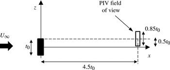
, with the PIV field of view centred as in figure 4 to measure the frequency of the Kármán vortex shedding.
Location of the measurements behind one of the largest bars, at
 $x/x_{\ast }^{peak}=0.08$
from the grid and centred at a
 $0.5t_{0}$
transverse (
 $z$
) distance from the bar’s centre.

2.3. Experimental technique
We use planar two-component PIV to measure the velocity field in the aforementioned stations. Figure 1 shows a schematic of the PIV system, which consists of a Nd:YLF laser (Litron LDY304 with
 $30~\text{mJ}/\text{pulse}$
at 1 kHz) with an output wavelength of 527 nm and a pair of CMOS cameras (Phantom v210). The cameras face the same interrogation area but with different magnifications, resulting in two different fields of view: small and large. Both fields of view are in the
 $xz$
plane and include the centreline (see figure 1).
The laser light sheet is obtained by bending the beam by 90° with a mirror, passing it through a spherical lens to converge the beam into a minimum thickness of approximately 1.2 mm (measured in Gomes-Fernandes et al. Reference Gomes-Fernandes, Ganapathisubramani and Vassilicos2014) and through a cylindrical lens to create the light sheet seen in figure 1.
For the large field of view (LFV), the cameras are operated at a resolution of
 $1280~\text{pixel}\times 800~\text{pixel}$
and are synchronised with the laser at a frequency of 500 Hz. They were fitted with a Nikon 60 mm lenses with an
 $f\#$
of 5.6. Five runs of 8216 vector fields were acquired using the LFV at
 $x/x_{\ast }^{peak}=0.20$
, 0.44 and 0.57. A summary of the resolution related to the LFV is shown in table 3, where the Kolmogorov scale
 ${\it\eta}=({\it\nu}^{3}/{\it\epsilon})^{1/4}$
, with
 ${\it\nu}$
being the water’s kinematic viscosity and
 ${\it\epsilon}$
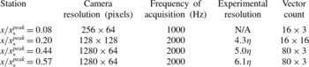
the turbulent kinetic energy dissipation. For the small field of view (SFV), the cameras operate at a resolution and frequency shown in table 4. Ten runs of 102 709 vector fields were acquired using this field of view at
 $x/x_{\ast }^{peak}=0.20$
, 0.44 and 0.57. The cameras were fitted with a Sigma 180 mm Macro lens with a
 $f\#$
of 8. For the station downstream of the thickest bar a Sigma 180 mm Macro lens is used with an
 $f\#$
of 5.6. The magnification was set to achieve a resolution close to
 $t_{0}/10$
to capture the secondary instabilities according to the DNS of Dong et al. (Reference Dong, Karniadakis, Ekmekci and Rockwell2006) at a similar Reynolds number compared with the present experiment (see table 2). Three runs of 513 600 vector fields were acquired at this station.
Experimental resolution computed with the LFV. The resolution is based on the Kolmogorov length scale at the centreline in the respective location.

Experimental resolution computed with the SFV. The resolution is based on the Kolmogorov length scale at the centreline in the respective location when applicable.

Distortion and other aberrations introduced by the lenses and water/glass interface are corrected using a calibration target with a fixed grid. A third-order polynomial function after Soloff, Adrian & Liu (Reference Soloff, Adrian and Liu1997) is fitted to map the vectors from image to object plane.
The flow is seeded with polyamide 12 powder with a nominal size of
 $7~{\rm\mu}\text{m}$
and a specific gravity of approximately 1.1. The response time (
 ${\it\tau}_{P}$
) of the seeding particles is estimated to be
 $0.24~{\rm\mu}\text{s}$
. The Stokes number
 $\mathit{St}={\it\tau}_{P}/{\it\tau}_{F}$
is estimated using the Kolmogorov time scale
 ${\it\tau}_{{\it\eta}}=\sqrt{{\it\nu}/{\it\epsilon}}$
as the characteristic time scale (
 ${\it\tau}_{F}$
). In our case
 $\mathit{St}=5\times 10^{-6}$
, which is substantially smaller than unity.
The images were acquired in single-frame mode. Frame 1 was correlated with frame 2 to get the first velocity field, frames 3 and 4 to get the second one, and so forth. The final interrogation window size was
 $32~\text{pixel}\times 32~\text{pixel}$
with 50 % overlap for the SFV and
 $16~\text{pixel}\times 16~\text{pixel}$
with 50 % overlap for the LFV. The total numbers of vectors for the large and small fields of view respectively are
 $3\times 80$
and
 $160\times 100$
in the
 $x\times y$
directions. The number of spurious vectors was less than 1 % for both fields of view. The time between frames allows an 8 pixel displacement on average.
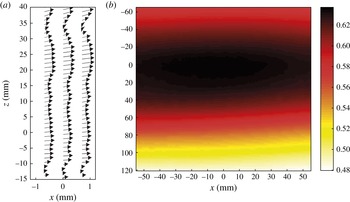
Figure 5 shows examples of the instantaneous fluctuating velocity field and the mean velocity field at
 $x/x_{\ast }^{peak}=0.44$
from the SFV and LFV respectively.
(a) Instantaneous fluctuating velocity field at
 $x/x_{\ast }^{peak}=0.44$
obtained from the SFV. Only half of the vector count is included in the
 $z$
direction. (b) Mean velocity field at
 $x/x_{\ast }^{peak}=0.44$
obtained from the LFV.

Using the SFV, the Taylor microscale
 ${\it\lambda}=\sqrt{\langle u^{2}\rangle /\langle (\partial u/\partial x)^{2}\rangle }$
(where
 $u\equiv u_{1}$
) is computed at
 $x/x_{\ast }^{peak}=0.44$
and 0.57, and it takes values of 7.2 mm and 10.3 mm respectively at the centrelines. The values of
 ${\it\lambda}$
do not change significantly across the
 $z$
direction, amounting to values between 6.5–7.3 mm and 9.2–11.2 mm for
 $x/x_{\ast }^{peak}=0.44$
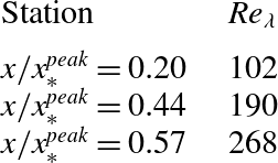
and 0.57 respectively. Table 5 shows the
 $\mathit{Re}_{{\it\lambda}}$
for the three stations measured in the production region.
Reynolds numbers
 $\mathit{Re}_{{\it\lambda}}=u^{\prime }{\it\lambda}/{\it\nu}$
, where
 $u^{\prime }$
is the r.m.s. of the streamwise velocity fluctuation,
 ${\it\lambda}=\sqrt{\langle u^{2}\rangle /\langle (\partial u/\partial x)^{2}\rangle }$
is the Taylor microscale and
 ${\it\nu}$
is the kinematic viscosity.

3. Energy spectra and third-order structure function
3.1. Energy spectra and data filtering
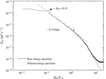
Figure 6 shows the one-dimensional longitudinal energy spectra
 $E_{11}$
in the frequency domain evaluated at
 $x/x_{\ast }^{peak}=0.44$
for
 $z=y=0$
, i.e. at the centreline, using raw and filtered data from the SFV. In the horizontal axis we show the frequency normalised by the lateral thickness of the largest bars,
 $t_{0}$
(see table 1), and the free-stream velocity,
 $U_{\infty }$
(see table 2). There is a one decade power law with an approximate
 $-5/3$
exponent at this location and even more clearly at
 $x/x_{\ast }^{peak}=0.57$
(see figure 8
a,b), even though Gomes-Fernandes et al. (Reference Gomes-Fernandes, Ganapathisubramani and Vassilicos2014) reported that at
 $x/x_{\ast }^{peak}=0.57$
on the centreline, vortex stretching only marginally dominates over vortex compression, whereas in the decay region (
 $x/x_{\ast }^{peak}=2.04$
) and in various reference cases reported in the literature (such as regular grid turbulence and atmospheric surface layer), vortex stretching dominates over vortex compression very significantly.
One-dimensional longitudinal energy spectra
 $E_{11}$
at the centreline position
 $x/x_{\ast }^{peak}=0.44$
from raw and filtered PIV data. The horizontal axis represents the frequencies normalised by the lateral thickness of the largest bars,
 $t_{0}$
, and the free-stream velocity,
 $U_{\infty }$
.

At
 $ft_{0}/U_{\infty }\gtrsim 10$
the spectra display a noise floor. In order to reduce the effect of noise in the velocity gradients, a filter is applied to the data. The filter consists of a Gaussian kernel applied to the temporal data with the full width of the experimental resolution (via Taylor’s hypothesis) at
 $1/e^{2}$
. The result is shown in figure 6, where the effect of noise is greatly reduced. The filter is also applied to the
 $w$
component of the measured fluctuating velocity and displays the same behaviour as the
 $u$
component.
The peak appearing approximately around
 $ft_{0}/U_{\infty }=0.13$
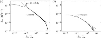
(see figure 6) is related to the initial conditions, more specifically to the Kármán vortex shedding of the largest bars. Figure 7(a) shows the one-dimensional longitudinal energy spectra downstream of the largest bar (see figure 4), centred in the
 $y$
direction at
 $x/x_{\ast }^{peak}=0.08$
, confirming that the peak at
 $\mathit{St}_{K}=0.13$
is related to the Kármán vortex shedding. It is also worth noting that the power-law exponent of the inertial range is close to 2, which is consistent with the vortex sheet structure of the flow at such a close distance to the grid. Regarding the second peak seen at
 $ft_{0}/U_{\infty }=1.3$
in figure 6, the same peak appears in the spectra at
 $x/x_{\ast }^{peak}=0.20$
when the grid is not in place (see figure 7
b), thus suggesting that its origin is not in the turbulence generated by the fractal grid.
(a) One-dimensional longitudinal energy spectra
 $E_{11}$
at the off-centreline position
 $x/x_{\ast }^{peak}=0.08$
shown in figure 4 downstream of one of the largest bars. (b) One-dimensional longitudinal energy spectra
 $E_{11}$
at
 $x/x_{\ast }^{peak}=0.20$
on the centreline without the grid in place. The horizontal axis represents the frequencies normalised by the lateral thickness of the largest bars,
 $t_{0}$
, and the free-stream velocity,
 $U_{\infty }$
.

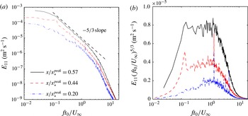
The spatial evolution of the one-dimensional spectra from station
 $x/x_{\ast }^{peak}=0.20$
, to
 $x/x_{\ast }^{peak}=0.44$
and eventually
 $x/x_{\ast }^{peak}=0.57$
is shown in figure 8(a,b) and corresponds to an evolution from
 $\mathit{Re}_{{\it\lambda}}=102$
, to
 $\mathit{Re}_{{\it\lambda}}=190$
and eventually
 $\mathit{Re}_{{\it\lambda}}=268$
(table 5). At
 $x/x_{\ast }^{peak}=0.20$
the Kármán vortex shedding signature is not present in this centreline spectrum, but it does appear at
 $x/x_{\ast }^{peak}=0.44$
. At
 $x/x_{\ast }^{peak}=0.44$
the spectrum has already a decade of scaling with exponent close to
 $-5/3$
(see the compensated spectra in figure 8
b). At
 $x/x_{\ast }^{peak}=0.57$
the existence of a decade of
 $-5/3$
scaling is very clear even though we are at the heart of the production region where the turbulence is highly inhomogeneous and the turbulence intensity is still rising with streamwise distance from the grid.
(a) Spatial evolution of the one-dimensional spectra at centreline positions
 $x/x_{\ast }^{peak}=0.20$
, 0.44 and 0.57 and (b) the same data compensated by
 $(\,ft_{0}/U_{\infty })^{5/3}$
in linear-logarithmic axes. The horizontal axis represents the frequencies normalised by the lateral thickness of the largest bars,
 $t_{0}$
, and the free-stream velocity,
 $U_{\infty }$
.

3.2. Third-order structure function and statistical convergence
The third-order structure function
 $\overline{{\it\delta}u_{\Vert }{\it\delta}q^{2}}$
can be calculated with
 $\boldsymbol{r}$
along the streamwise direction, i.e.
 $\boldsymbol{r}=(r_{1},0,0)$
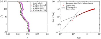
, by making use of the Taylor hypothesis in this direction. We established the validity of this hypothesis at
 $x/x_{\ast }^{peak}=0.44$
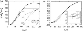
and 0.57, and we present details of this validation in appendix A. In figure 9 we plot this third-order structure function, which we have calculated by assuming that
 $\overline{{\it\delta}u{\it\delta}q^{2}}\approx \overline{{\it\delta}u^{3}}+2\overline{{\it\delta}u{\it\delta}w^{2}}$
(where
 $u\equiv u_{1}$
,
 $v\equiv u_{2}$
and
 $w\equiv u_{3}$
). In this figure,
 $\overline{{\it\delta}u_{\Vert }{\it\delta}q^{2}}=\overline{{\it\delta}u{\it\delta}q^{2}}$
is normalised by the Kolmogorov velocity scale
 $u_{k}=({\it\nu}{\it\epsilon})^{1/4}$
and is plotted as a function of the normalised streamwise separation scale
 $r_{1}/{\it\eta}$
. It is of course legitimate to plot
 $\overline{{\it\delta}u{\it\delta}q^{2}}$
as a function of
 $r_{1}$
in principle, but it must be stressed that this plot will be representative of
 $\overline{{\it\delta}u_{\Vert }{\it\delta}q^{2}}$
as a function of
 $r$
for any direction
 $\boldsymbol{r}/r$
only if the small scales are isotropic in the sense defined in the introduction when proceeding from (1.6) and (1.7).
Third-order structure function
 $\langle {\it\delta}u{\it\delta}q^{2}\rangle$
(where
 ${\it\delta}q^{2}={\it\delta}u^{2}+2{\it\delta}w^{2}$
) normalised by the Kolmogorov velocity
 $u_{k}$
versus the streamwise separation
 $r_{1}$
normalised by the Kolmogorov length
 ${\it\eta}$
at (a)
 $x/x_{\ast }^{peak}=0.44$
and (b)
 $x/x_{\ast }^{peak}=0.57$
. Error bars represent a 95 % confidence interval for the true value.

The inset in figure 9(a) shows the same data in a logarithmic scale to stress that the small scales do indeed follow a power law
 $\propto r^{3}$
, as would be expected by straightforward Taylor expansion if the resolution is adequate. In this inset we also include a straight line representing a power law of exponent 1 for comparison with the
 $r$
dependence in (1.7).
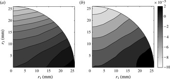
The most striking observation made when looking at figure 9 is that
 $\overline{{\it\delta}u{\it\delta}q^{2}}$
is positive throughout the range of separations
 $r_{1}$
at
 $x/x_{\ast }^{peak}=0.44$
and
 $x/x_{\ast }^{peak}=0.57$
(even though at
 $x/x_{\ast }^{peak}=0.57$
it is not possible to confirm this within a confidence interval for
 $r/{\it\eta}$
less than approximately 40, see the inset of figure 9
b). This would imply an inverse energy cascade, i.e. from small to large scales, if the small-scale turbulent fluctuations were isotropic in the sense that (1.6) could be used to imply (1.7). As they are not (see § 5), there remains the possibility that the interscale energy transfers are anisotropic, allowing for a forward cascade in one direction and an inverse one in the other.
It is therefore important to show that
 $\overline{{\it\delta}u{\it\delta}q^{2}}$
is positive within a confidence interval. We choose a 95 % confidence interval and use the expression
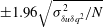 $\pm 1.96\sqrt{{\it\sigma}_{{\it\delta}u{\it\delta}q^{2}}^{2}/N}$
, where
 ${\it\sigma}_{{\it\delta}u{\it\delta}q^{2}}^{2}$
is the variance of
 ${\it\delta}u{\it\delta}q^{2}$
and
 $N$
is the number of independent samples. The number of independent samples is chosen on the basis of a bespoke integral length scale calculated for this purpose by integrating the correlation function of
 ${\it\delta}u{\it\delta}q^{2}(r_{1},r_{3})$
as in Valente & Vassilicos (Reference Valente and Vassilicos2015). The number of independent samples is then estimated by choosing points separated by at least two such bespoke integral length scales, resulting in the confidence intervals seen in figure 9. We conclude that
 $\langle {\it\delta}u{\it\delta}q^{2}\rangle$
is indeed positive within the chosen 95 % confidence interval and that statistical convergence, at least for the sign of
 $\langle {\it\delta}u{\it\delta}q^{2}\rangle$
, has therefore been achieved.
4. Data reduction
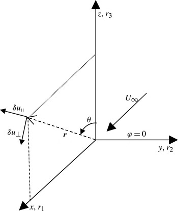
In the present planar PIV experiment the two-point separation vectors are in the PIV
 $xz$
plane. The streamwise component of the separation,
 $r_{1}$
, is evaluated along the
 $x$
direction, and the transverse component,
 $r_{3}$
, along the
 $z$
direction (see figure 10). In order to obtain the terms in (1.2) some assumptions are made because 2D planar PIV does not provide information about the third velocity component (in our case
 $v$
in the
 $y$
direction) and about how the second- and third-order structure functions behave in the
 $y$
direction. Therefore we assume
 $\overline{{\it\delta}v^{2}}=\overline{{\it\delta}w^{2}}$
, which implies
 $\overline{{\it\delta}q^{2}}(\boldsymbol{r})=\overline{{\it\delta}u^{2}}(\boldsymbol{r})+2\overline{{\it\delta}w^{2}}(\boldsymbol{r})$
, and that the interscale flux vector can be approximated as
 $\overline{{\it\delta}u_{i}{\it\delta}q^{2}}(\boldsymbol{r})\approx \overline{{\it\delta}u_{i}{\it\delta}u^{2}}(\boldsymbol{r})+2\overline{{\it\delta}u_{i}{\it\delta}w^{2}}(\boldsymbol{r})$
.
The coordinate system. The velocity difference components
 ${\it\delta}u_{\Vert }$
and
 ${\it\delta}u_{\bot }$
lie on the measurement PIV plane. The angle between the
 $r_{3}$
axis and
 $\boldsymbol{r}$
is denoted
 ${\it\theta}$
.

The various terms in (1.2) are estimated by calculating the following statistics, where the average is over time:
 $\overline{{\it\delta}u^{2}}$
,
 $\overline{{\it\delta}w^{2}}$
,
 $\overline{{\it\delta}u^{3}}$
,
 $\overline{{\it\delta}w^{3}}$
,
 $\overline{{\it\delta}u{\it\delta}w^{2}}$
,
 $\overline{{\it\delta}w{\it\delta}u^{2}}$
,
 $\overline{(w+w^{\prime }){\it\delta}u}$
,
 $\overline{(u+u^{\prime }){\it\delta}u^{2}}$
,
 $\overline{(w+w^{\prime }){\it\delta}u^{2}}$
,
 $\overline{(u+u^{\prime }){\it\delta}w^{2}}$
and
 $\overline{(w+w^{\prime }){\it\delta}w^{2}}$
at the two centroids
 $\boldsymbol{X}=(0.44x_{\ast }^{peak},0,0)$
and
 $\boldsymbol{X}=(0.57x_{\ast }^{peak},0,0)$
for many different separation vectors
 $(r_{1},r_{3})$
. Hence, (1.2) is evaluated at the two aforementioned centroids both along the centreline of the tunnel. In the
 $z$
direction,
 $r_{3}$
is limited by the SFV and attains a maximum value of 26 mm (see figure 5
a). In the
 $x$
direction,
 $r_{1}$
is obtained from Taylor’s hypothesis and is sampled to take similar values to our separations
 $r_{3}$
.
All statistics are then bilinearly interpolated into a spherical coordinate system where
 $r_{1}$
is aligned with
 $(r,{\rm\pi}/2,0)$
and
 $r_{3}$
with
 $(r,0,0)$
in the
 $(r,{\it\theta},{\it\phi}=0)$
plane (see figure 10). The spherical coordinate grid results from the intersections of 19 equally spaced circumferences with 19 equally spaced radial lines between
 ${\it\theta}=0$
and
 ${\it\theta}={\rm\pi}/2$
.
Our planar PIV can only access
 ${\it\delta}u$
and
 ${\it\delta}w$
. Therefore, we use DNS data of Laizet & Vassilicos (Reference Laizet and Vassilicos2015) to verify the assumption
 $\overline{{\it\delta}v^{2}}=\overline{{\it\delta}w^{2}}$
. The data we use are from their DNS1–5, which are numerical simulations of turbulence generated by a fractal grid very similar to ours, except that it has
 $N=3$
fractal iterations and a thickness ratio
 $t_{r}=8.4$
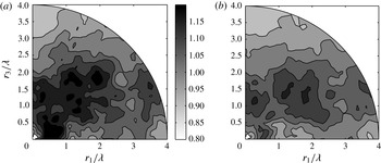
. Figure 11 shows the ratio
 $(\overline{{\it\delta}u^{2}}(\boldsymbol{r})+\overline{{\it\delta}v^{2}}(\boldsymbol{r})+\overline{{\it\delta}w^{2}}(\boldsymbol{r}))/(\overline{{\it\delta}u^{2}}(\boldsymbol{r})+2\overline{{\it\delta}w^{2}}(\boldsymbol{r}))$
for different
 $r_{1}$
and
 $r_{3}$
centred at
 $x/x^{peak}=0.44$
(
 $x^{peak}$
is the actual exact location of the turbulence intensity peak along the centreline). This position corresponds to one of the two ceontroids considered here. We use 960 time steps in total to calculate statistics. Figure 11(a) shows the results obtained using half of these time steps and figure 11(b) shows the results obtained with all of them. The ratio
 $(\overline{{\it\delta}u^{2}}(\boldsymbol{r})+\overline{{\it\delta}v^{2}}(\boldsymbol{r})+\overline{{\it\delta}w^{2}}(\boldsymbol{r}))/(\overline{{\it\delta}u^{2}}(\boldsymbol{r})+2\overline{{\it\delta}w^{2}}(\boldsymbol{r}))$
varies between 0.85 and 1.15 in figure 11(b), which supports our assumption for the calculation of
 $\overline{{\it\delta}q^{2}}(\boldsymbol{r})$
. It is also evident from these results that these DNS data are not sufficient to converge higher-order statistics and therefore do not allow us to test our second assumption that the interscale flux vector can be approximated as
 $\overline{{\it\delta}u_{i}{\it\delta}q^{2}}(\boldsymbol{r})\approx \overline{{\it\delta}u_{i}{\it\delta}u^{2}}(\boldsymbol{r})+2\overline{{\it\delta}u_{i}{\it\delta}w^{2}}(\boldsymbol{r})$
.
Isocontours of the ratio
 $(\overline{{\it\delta}u^{2}}(\boldsymbol{r})+\overline{{\it\delta}v^{2}}(\boldsymbol{r})+\overline{{\it\delta}w^{2}}(\boldsymbol{r}))/(\overline{{\it\delta}u^{2}}(\boldsymbol{r})+2\overline{{\it\delta}w^{2}}(\boldsymbol{r}))$
using (a) 480 time steps and (b) 960 time steps. Data of Laizet & Vassilicos (Reference Laizet and Vassilicos2015).

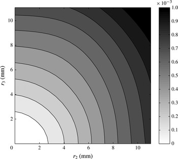
Map of
 $\overline{({\it\delta}\boldsymbol{u}\boldsymbol{\cdot }\hat{r}_{\vdash })^{2}}$
, in the
 $r_{2}r_{3}$
plane obtained at
 $x/x_{\ast }^{peak}=0.57$
, where
 $\hat{r}_{\vdash }$
is a unit vector normal to the directions marked
 ${\it\delta}u_{\Vert }$
and
 ${\it\delta}u_{\bot }$
in figure 10. We used the data presented in Gomes-Fernandes et al. (Reference Gomes-Fernandes, Ganapathisubramani and Vassilicos2014) and an additional two runs of data at the same location in order to converge the statistics.

All the terms in (1.2) are computed apart from the pressure transport. The derivatives with respect to
 $X_{1}$
and
 $X_{3}$
are computed using a first-order forward difference scheme from data at
 $x/x_{\ast }^{peak}=0.57$
and
 $x/x_{\ast }^{peak}=0.44$
. However, the derivatives with respect to
 $r_{1}$
and
 $r_{3}$
are computed using a second-order central difference scheme (except at the borders where
 $r_{1}=0$
or
 $r_{3}=0$
where we use a first-order forward difference scheme). Each term is estimated using approximations as in Valente & Vassilicos (Reference Valente and Vassilicos2015) which are detailed as follows.
-
(i)
$\mathscr{A}_{t}=0$
because of statistical stationarity and the nature of our averaging operation. -
(ii)
$4\mathscr{A}\approx (U+U^{\prime })/2\partial \overline{{\it\delta}q^{2}}/\partial X_{1}$
because
$V$
and
$W$
are less than 2 % of
$U$
and, therefore, are considered to be negligible. The gradient of the mean velocity in the
$x$
direction is found to be one order of magnitude smaller than in the
$z$
direction (see figure 5
b), hence the following approximation is used:
$(U+U^{\prime })/2\approx (U(X_{1},0,X_{3}+r_{3}/2)+U(X_{1},0,X_{3}-r_{3}/2))/2$
. We calculate
$4\mathscr{A}$
only at
$x/x_{peak}^{\ast }=0.44$
because we need the data at
$x/x_{peak}^{\ast }=0.57$
to estimate the derivative with respect to
$X_{1}$
. The mean flow data were taken from the LFV seen in figure 5(b). -
(iii)
$4{\it\Pi}\approx 1/r^{2}\partial /\partial r(r^{2}\overline{{\it\delta}u_{\Vert }{\it\delta}q^{2}})+1/(r\sin {\it\theta})\partial /\partial {\it\theta}(\sin {\it\theta}\overline{{\it\delta}u_{\bot }{\it\delta}q^{2}})$
, where
${\it\delta}u_{\Vert }$
and
${\it\delta}u_{\bot }$
are the longitudinal and transverse velocity differences shown in figure 10. The divergence of the energy flux is estimated in spherical coordinates where the contribution from the
$\partial /\partial {\it\phi}$
term is neglected because we assume the energy flux component in the direction (defined by the unit vector
$\hat{\boldsymbol{r}}_{\vdash }$
) normal to the directions marked
${\it\delta}u_{\Vert }$
and
${\it\delta}u_{\bot }$
in figure 10 to be approximately independent of the angle
${\it\phi}$
. We cannot test this assumption directly. However, we can use the data of Gomes-Fernandes et al. (Reference Gomes-Fernandes, Ganapathisubramani and Vassilicos2014) to plot
$\overline{({\it\delta}\boldsymbol{u}\boldsymbol{\cdot }\hat{r}_{\vdash })^{2}}$
at
$x/x_{\ast }^{peak}=0.57$
in the
$r_{2}r_{3}$
plane and see whether this quantity is approximately independent of
${\it\phi}$
(figure 12). Unfortunately the data of Gomes-Fernandes et al. (Reference Gomes-Fernandes, Ganapathisubramani and Vassilicos2014) are insufficient to converge third-order statistics such as the relevant component of the energy flux, but figure 12 does provide some indirect support for our assumption, albeit on another, yet related, quantity. The wind tunnel experiments on turbulence generated by the same fractal square grid reported by Nagata et al. (Reference Nagata, Sakai, Suzuki, Suzuki, Terashima and Inaba2013) also support this assumption. These authors found that the one-point kinetic energy and the skewness of the streamwise fluctuating velocity are approximately axisymmetric around the centreline in the production region (and specifically at streamwise distances from the grid very similar to ours in terms of fractions of
$x_{peak}^{\ast }$
) within a radius smaller than 5 % of the tunnel width. The maximum separation
$r~({\approx}26~\text{mm})$
considered in the present statistics is always smaller than 5 % of our channel width, and it is reasonable to assume that the two-point statistics involved in the definition of
$4{\it\Pi}$
should also be axisymmetric under such conditions. We calculate
$4{\it\Pi}$
at both
$x/x_{peak}^{\ast }=0.44$
and 0.57 where the field of view is wide enough in the
$r_{3}$
direction. -
(iv)
$4{\it\Pi}_{U}\approx \partial {\it\delta}U\overline{{\it\delta}q^{2}}/\partial r_{1}$
, where we effectively assume
$V=W=0$
as we are on the centreline or very near it. Due to centreline symmetry,
$U(X_{1},0,r_{3}/2)\approx U(X_{1},0,-r_{3}/2)$
and
${\it\delta}U$
is only non-zero for
$r_{3}\neq 0$
. Since
$U$
is a slowly varying function of
$x$
(or
$X_{1}$
) we approximate
${\it\delta}U$
with a Taylor expansion
${\it\delta}U\approx r_{1}\partial U/\partial x$
and we use a second-order central difference scheme to estimate it at
$x/x_{peak}^{\ast }=0.44$
with data from
$x/x_{\ast }^{peak}=0.20$
and 0.57. -
(v)
$4\mathscr{P}\approx 2\overline{{\it\delta}u^{2}}\partial U/\partial x+2\overline{(w+w^{\prime }){\it\delta}u}\partial U/\partial z$
, as
$V$
and
$W$
are again assumed equal to zero as well as
$\partial U/\partial y$
and
$\partial U^{\prime }/\partial y^{\prime }$
because of the mean flow symmetry in the
$xz$
plane. In addition, symmetry of the flow in relation to the centreline is invoked as
$\partial U/\partial z\approx -\partial U^{\prime }/\partial z^{\prime }$
as well as the approximation that
$\partial U/\partial x\approx \partial U^{\prime }/\partial x^{\prime }$
. The gradient
$\partial U/\partial z$
is taken from a second-degree polynomial function fitted to the data in figure 5(b) at
$x/{\it\eta}=0$
. -
(vi)
$4\mathscr{T}\approx -\partial /\partial X_{1}(\overline{(u+u^{\prime }){\it\delta}q^{2}}/2)-\partial /\partial X_{3}(\overline{(w+w^{\prime }){\it\delta}q^{2}})$
, where the derivative in
$X_{3}$
,
$\partial /\partial X_{3}(\overline{(w+w^{\prime }){\it\delta}q^{2}}/2)$
, is assumed to be equal to
$\partial /\partial X_{2}(\overline{(v+v^{\prime }){\it\delta}q^{2}}/2)$
given the 90° statistical flow symmetry about the centreline. The transverse derivative is estimated by taking another centroid along the
$z$
axis where
$z=13~\text{mm}$
(see figure 5
a). The results were checked and were found not to be significantly sensitive to the
$z$
coordinate chosen around this value. The term
$4\mathscr{T}$
was estimated at
$x/x_{peak}^{\ast }=0.44$
using data from
$x/x_{\ast }^{peak}=0.57$
. -
(vii) The pressure transport
$4\mathscr{T}_{p}$
cannot be estimated with the present data. -
(viii)
$4\mathscr{D}_{{\it\nu}}\approx 2{\it\nu}/r^{2}\partial /\partial r(r^{2}\partial \overline{{\it\delta}q^{2}}/\partial r)$
plus polar and azimuthal contributions which cancel out when averaged over spherical shells. Here, we only calculate the radial contribution to
$4\mathscr{D}_{{\it\nu}}$
at
$x/x_{peak}^{\ast }=0.44$
and 0.57. It should be noted that
$4\mathscr{D}_{{\it\nu}}$
tends to
${\it\epsilon}(\boldsymbol{X})$
when the scale separation tends to zero. It was also mathematically shown in Laizet et al. (Reference Laizet, Vassilicos and Cambon2013) and Valente & Vassilicos (Reference Valente and Vassilicos2015) that
$4\mathscr{D}_{{\it\nu}}$
is small compared with
${\it\epsilon}(\boldsymbol{X})$
when
$r$
is larger than the Taylor microscale. -
(ix)
$4\mathscr{D}_{X,{\it\nu}}\approx {\it\nu}/2\partial ^{2}/\partial X_{1}^{2}(\overline{{\it\delta}q^{2}})+{\it\nu}\partial ^{2}/\partial X_{3}^{2}(\overline{{\it\delta}q^{2}})$
, where use is again made of 90° symmetry about the centreline. The streamwise second-order derivative is only computed for
$r_{3}=0$
using data from stations
$x/x_{\ast }^{peak}=0.20$
, 0.44 and 0.57. Hence we estimate
$4\mathscr{D}_{X,{\it\nu}}$
only at
$x/x_{\ast }^{peak}=0.44$
. Valente & Vassilicos (Reference Valente and Vassilicos2015) reported that this term is negligibly small for the decay region of regular grids, and we confirm that the same holds in the production region of our fractal grid by calculating this term for several
$r_{1}$
separations (see § 6). The second-order derivative in the
$z$
direction (assumed to be equal to the one in the
$y$
direction, given the 90° symmetry) is estimated using the statistical symmetry with respect to the centreline in the
$zx$
plane, where it becomes
$2(\overline{{\it\delta}q^{2}}(X_{1},0,{\rm\Delta}z;\boldsymbol{r})-\overline{{\it\delta}q^{2}}(X_{1},0,0;\boldsymbol{r}))/{\rm\Delta}z^{2}$
(
${\rm\Delta}z=13~\text{mm}$
). -
(x)
$4{\it\epsilon}^{\ast }=4({\it\epsilon}+{\it\epsilon}^{\prime })/2$
, where we use the surrogate
$3{\it\nu}(\overline{s_{11}^{2}}+\overline{s_{22}^{2}})+12{\it\nu}\overline{s_{12}^{2}}$
with
$s_{ij}=(\partial u_{i}/\partial x_{j}+\partial u_{j}/\partial x_{i})/2$
(Tanaka & Eaton Reference Tanaka and Eaton2007) to estimate the energy dissipation at
$\boldsymbol{x}$
and
$\boldsymbol{x}^{\prime }$
. To estimate
${\it\epsilon}$
and
${\it\epsilon}^{\prime }$
from the SFV, which does not allow
$r_{1}$
values beyond the resolution scale, we use the observation that
${\it\epsilon}$
and
${\it\epsilon}^{\prime }$
are about equal along a
$z=\text{const.}$
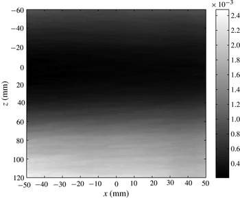
line. This observation is supported by figure 13, where we plot an
$xz$
map of
${\it\epsilon}$
calculated from the LFV at
$x/x_{peak}^{\ast }=0.44$
. This figure shows clearly that
${\it\epsilon}$
varies significantly along
$z$
but very little along
$x$
. Even though the spatial resolution in this figure is relatively low (close to
$8.4{\it\eta}$
on the centreline, see table 3), we do not expect the qualitative behaviour to change much with increased resolution. -
(xi)
$4\mathscr{B}=4\mathscr{A}+4{\it\Pi}+4{\it\Pi}_{U}-4\mathscr{P}-4\mathscr{T}-4\mathscr{D}_{{\it\nu}}-4\mathscr{D}_{X,{\it\nu}}+4{\it\epsilon}^{\ast }$
, where each one of these terms is calculated as described in the preceding points. Therefore,
$4\mathscr{B}$
is the remainder required to satisfy the Kármán–Howarth balance (1.2). This remainder may be expected to be dominated by the pressure transport
$4\mathscr{T}_{p}$
, which we are unable to measure, but it can also have contributions coming from the simplifying assumptions we made when estimating all the other terms.












































Turbulent energy dissipation
 ${\it\epsilon}~(\text{m}^{4}~\text{s}^{-3})$
map in the
 $xz$
plane at
 $x/x_{\ast }^{peak}=0.44$
.

5. Nonlinear energy transfer between scales
Having obtained positive values for
 $\overline{{\it\delta}u{\it\delta}q^{2}}$
(figure 9), we now plot isocontours of
 $\overline{{\it\delta}u_{\Vert }{\it\delta}q^{2}}$
which show how this quantity depends on
 $r_{1}$
and
 $r_{3}$
at
 $x/x_{\ast }^{peak}=0.44$
and 0.57. This map (figure 14) shows that
 $\overline{{\it\delta}u_{\Vert }{\it\delta}q^{2}}$
is not isotropic at the scales considered and is therefore different from
 $\overline{{\it\delta}u{\it\delta}q^{2}}$
. Hence, (1.7) does not follow from (1.6) at the locations where we measure in this turbulent flow and must not be expected to hold. In fact, figure 14 shows that
 $\overline{{\it\delta}u_{\Vert }{\it\delta}q^{2}}$
has different signs at different values of
 $(r_{1},r_{3})$
, which invalidates (1.7) at a stroke.
Isocontours of the parallel third-order structure function
 $\overline{{\it\delta}u_{\Vert }{\it\delta}q^{2}}~(\text{m}^{3}~\text{s}^{-3})$
at (a)
 $x/x_{\ast }^{peak}=0.44$
and (b)
 $x/x_{\ast }^{peak}=0.57$
.

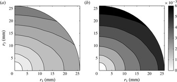
Figure 15 shows the isocontours of the second-order structure function
 $\overline{{\it\delta}q^{2}}(r_{1},r_{3})$
at
 $x/x_{\ast }^{peak}=0.44$
and 0.57. It may be interesting to note that
 $\overline{{\it\delta}q^{2}}(r_{1},r_{3})$
is much more isotropic than
 $\overline{{\it\delta}u_{\Vert }{\it\delta}q^{2}}$
. In fact, in terms of spherical coordinates (see figure 10), the variation of
 $\overline{{\it\delta}q^{2}}(r,{\it\theta},{\it\phi}=0)$
with angle
 ${\it\theta}$
shows that
 $\overline{{\it\delta}q^{2}}$
becomes more isotropic from
 $x/x_{\ast }^{peak}=0.44$
to 0.57 as the isocontours become more circular. It should be noted also that in the production region where the present measurements are taken, the turbulence intensity increases along the streamwise direction and so does the energy contained within a specific separation vector
 $(r_{1},r_{3})$
in figure 15.
Isocontours of the second-order structure function
 $\overline{{\it\delta}q^{2}}~(\text{m}^{2}~\text{s}^{-2})$
at (a)
 $x/x_{\ast }^{peak}=0.44$
and (b)
 $x/x_{\ast }^{peak}=0.57$
.

The possibility of a forward cascade in one direction and an inverse cascade in the other has already been mentioned in § 3.2, and the different signs of
 $\overline{{\it\delta}u_{\Vert }{\it\delta}q^{2}}$
for different separation vectors
 $(r_{1},r_{3})$
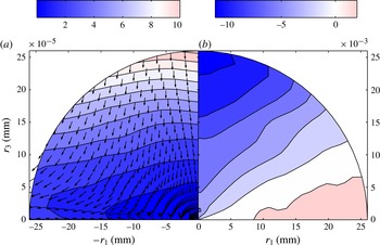
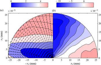
in figure 14 support such a view. Following Lamriben, Cortet & Moisy (Reference Lamriben, Cortet and Moisy2011) and Valente & Vassilicos (Reference Valente and Vassilicos2015), we plot the fluxes
 $\overline{{\it\delta}u_{i}{\it\delta}q^{2}}$
in figures 16(a) and 17(a) for
 $x/x_{\ast }^{peak}=0.44$
and 0.57 respectively. The directions of these flux vectors show an inverse cascade roughly aligned with an axis at a small angle from the streamwise (
 $r_{1}$
and velocity component
 $u$
) direction, and a forward cascade roughly aligned in the lateral (
 $r_{3}$
and velocity component
 $w$
) direction for
 $r_{1}$
is small. For separation vectors between these two extremes, the interscale energy flux is in an intermediate state where the cascade is both forward and inverse in different components of the flux vector, i.e. forward in the longitudinal and inverse in the streamwise projections of this vector. For separation vectors between the streamwise direction and the aforementioned axis at a slight angle to this direction, the cascade is purely inverse.
(a) Third-order structure function vectors
 $\overline{{\it\delta}u_{i}{\it\delta}q^{2}}$
and isocontours of their magnitude and (b) isocontours of the radial part of the divergence of
 $\overline{{\it\delta}u_{i}{\it\delta}q^{2}}$
at
 $x/x_{\ast }^{peak}=0.44$
.

Writing the nonlinear energy transfer term
 $4{\it\Pi}(\boldsymbol{X},\boldsymbol{r})=\partial \overline{{\it\delta}u_{i}{\it\delta}q^{2}}/\partial r_{i}$
in spherical coordinates as in § 4 and integrating over the solid angle one immediately obtains
 $$\begin{eqnarray}\int 4{\it\Pi}\,\text{d}{\it\Omega}=\int 4{\it\Pi}_{r}\,\text{d}{\it\Omega},\end{eqnarray}$$
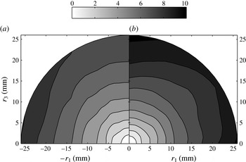
where
 ${\it\Pi}_{r}=1/r^{2}\partial /\partial r(r^{2}\overline{{\it\delta}u_{\Vert }{\it\delta}q^{2}})$
is the radial part of the divergence of
 $\overline{{\it\delta}u_{i}{\it\delta}q^{2}}$
. This relation between two integrals simply states that when averaged over all directions, the nonlinear interscale energy transfers are fully determined only by the radial part
 ${\it\Pi}_{r}$
of the interscale flux divergence. We therefore plot
 ${\it\Pi}_{r}$
in figures 16(b) and 17(b) but remain mindful of the limitations imposed by our measurement capabilities which mean that we can only plot isocontours of
 ${\it\Pi}_{r}$
in the
 ${\it\phi}=0$
plane (see figure 10). The white contour indicates the transition between negative and positive values for
 ${\it\Pi}_{r}$
in agreement with the behaviour of the flux vectors. This is another way to extract from the data the information that the cascade in the two production region locations considered here is both forward and inverse, the inverse part operating mostly in the streamwise direction whereas the forward part operates mostly in the lateral direction along
 $z$
.
(a) Third-order structure function vectors
 $\overline{{\it\delta}u_{i}{\it\delta}q^{2}}$
and isocontours of their magnitude and (b) isocontours of the radial part of the divergence of
 $\overline{{\it\delta}u_{i}{\it\delta}q^{2}}$
at
 $x/x_{\ast }^{peak}=0.57$
.

It may be worth pointing out that the energy spectra at the centreline positions
 $x/x_{\ast }^{peak}=0.44$
and
 $x/x_{\ast }^{peak}=0.57$
where we find this combination of forward and inverse cascades have power-law spectra with exponents close to
 $-5/3$
(see figure 8
a,b). In fact the inverse part of the cascade is around the streamwise direction. This is also the direction for which these
 $E_{11}(k_{1})$
energy spectra are calculated, the wavenumber
 $k_{1}$
corresponding to the frequency
 $f$
in figure 8 by Taylor’s hypothesis
 $k_{1}=fU_{1}$
(see appendix A for our validation of the Taylor hypothesis in the present context).
To evaluate whether the cascade is overall forward or inverse at a given separation
 $|\boldsymbol{r}|=r$
, we need to integrate
 ${\it\Pi}$
over the angles
 ${\it\theta}$
and
 ${\it\phi}$
(see figure 10). However, our data do not allow us to calculate the integrals in (5.1) because they are confined to the plane
 ${\it\phi}=0$
. Nevertheless, we can calculate
 $\int _{0}^{{\rm\pi}/2}{\it\Pi}\,\text{d}{\it\theta}$
and
 $\int _{0}^{{\rm\pi}/2}{\it\Pi}_{r}\,\text{d}{\it\theta}$
using the reduced form for
 ${\it\Pi}$
in § 4. We find these two integrals to be very close to each other at both centreline positions
 $x/x_{\ast }^{peak}=0.44$
and
 $x/x_{\ast }^{peak}=0.57$
. In fact, Laizet & Vassilicos (Reference Laizet and Vassilicos2011) and Nagata et al. (Reference Nagata, Sakai, Suzuki, Suzuki, Terashima and Inaba2013) have shown that in a transverse planar region around the centreline of size less than approximately
 $L_{0}/10$
at these positions (
 $L_{0}/10$
corresponds to approximately 30 mm here) the one-point turbulence statistics are approximately axisymmetric around the streamwise axis, i.e. independent of
 ${\it\phi}$
. Their result is consistent with our finding that
 $\int _{0}^{{\rm\pi}/2}{\it\Pi}\,\text{d}{\it\theta}\approx \int _{0}^{{\rm\pi}/2}{\it\Pi}_{r}\,\text{d}{\it\theta}$
, which is implied from (5.1) when
 ${\it\Pi}$
and
 ${\it\Pi}_{r}$
are independent of the angle
 ${\it\phi}$
.
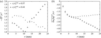
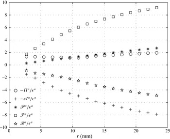
In figure 18(a) we plot
 $-{\it\Pi}^{a}\equiv -(2/{\rm\pi})\int _{0}^{{\rm\pi}/2}{\it\Pi}\,\text{d}{\it\theta}$
normalised by
 ${\it\epsilon}^{a}\equiv (2/{\rm\pi})\int _{0}^{{\rm\pi}/2}{\it\epsilon}^{\ast }\,\text{d}{\it\theta}$
as a function of
 $r=|\boldsymbol{r}|$
. The first observation is that, regardless of the inverse and forward cascade mix evident in the previous statistics, the sign of
 ${\it\Pi}^{a}$
is negative for all separations
 $r$
considered here. This indicates an overall forward cascade when integrated over the different directions. The second observation is that
 $-{\it\Pi}^{a}/{\it\epsilon}^{a}$
takes values between 1 and 2 at
 $x/x_{\ast }^{peak}=0.44$
and between 1.1 and 1.6 at
 $x/x_{\ast }^{peak}=0.57$
where the
 $-5/3$
spectrum is particularly well defined (see figure 8). It should be noted that when we normalise
 $-{\it\Pi}^{a}$
by
 ${\it\epsilon}$
(i.e.
 ${\it\epsilon}^{\ast }$
at
 $\boldsymbol{r}=\mathbf{0}$
), the plots in figure 18(a) do not change much and, in fact, for the case where
 $x/x_{\ast }^{peak}=0.57$
,
 $-{\it\Pi}^{a}/{\it\epsilon}$
varies between 1.2 and 1.5. There is therefore some tendency for
 $-{\it\Pi}^{a}$
to be close to a constant at
 $x/x_{\ast }^{peak}=0.57$
, though far from perfectly so. This suggests a cascade that is approximately self-similar in scales when directions have been integrated out.
(a) The circumferentially averaged nonlinear energy transfer term
 ${\it\Pi}^{a}$
normalised by the similarly averaged energy dissipation
 ${\it\epsilon}^{a}$
. (b) The circumferentially averaged parallel third-order structure function compensated by
 ${\it\epsilon}^{a}r$
, i.e.
 $\overline{{\it\delta}u_{\Vert }{\it\delta}q^{2}}^{a}/{\it\epsilon}r$
as a function of
 $r$
(mm), at
 $x/x_{\ast }^{peak}=0.44$
and
 $x/x_{\ast }^{peak}=0.57$
.

A functional form for the directionally averaged interscale flux
 $\overline{{\it\delta}u_{\Vert }{\it\delta}q^{2}}^{a}=(2/{\rm\pi})\int _{0}^{{\rm\pi}/2}\overline{{\it\delta}u_{\Vert }{\it\delta}q^{2}}\,\text{d}{\it\theta}$
can be derived from the observation that
 $-{\it\Pi}^{a}$
is not too far from a constant and using
 $r^{2}4{\it\Pi}^{a}=(2/{\rm\pi})\int _{0}^{{\rm\pi}/2}(\partial /\partial r)(r^{2}\overline{{\it\delta}u_{\Vert }{\it\delta}q^{2}})\,\text{d}{\it\theta}=(\partial /\partial r)(r^{2}\overline{{\it\delta}u_{\Vert }{\it\delta}q^{2}}^{a})$
. Integrating with respect to
 $r$
(starting from
 $r=0$
) while assuming that
 ${\it\Pi}^{a}$
is constant yields
 $$\begin{eqnarray}\overline{{\it\delta}u_{\Vert }{\it\delta}q^{2}}^{a}=4{\it\Pi}^{a}r/3.\end{eqnarray}$$
In figure 18(b) we plot
 $\overline{{\it\delta}u_{\Vert }{\it\delta}q^{2}}^{a}/({\it\epsilon}r)$
versus
 $r$
and see that, at
 $x/x_{\ast }^{peak}=0.57$
where the
 $-5/3$
is most clearly present (figure 8),
 $\overline{{\it\delta}u_{\Vert }{\it\delta}q^{2}}^{a}\approx -16{\it\epsilon}r/9$
(consistent with (5.2) and
 ${\it\Pi}^{a}\approx -4{\it\epsilon}/3$
from figure 18
a) but with a small drift away from this expression. Hence, even though (1.7) does not hold here, a relation similar to it does hold at
 $x/x_{\ast }^{peak}=0.57$
when averaging over separation vector orientations. (It should be noted also that figure 18
b remains roughly the same when plotting
 $\overline{{\it\delta}u_{\Vert }{\it\delta}q^{2}}^{a}/({\it\epsilon}^{a}r)$
rather than
 $\overline{{\it\delta}u_{\Vert }{\it\delta}q^{2}}^{a}/({\it\epsilon}r)$
.)
We now make a final set of observations which relate to (1.5) in the introduction. This equation is central to the Richardson–Kolmogorov cascade and is typically derived by assuming local homogeneity and local equilibrium (1.5). It implies, in particular, that the nonlinear energy transfer term (or divergence of the interscale energy flux)
 ${\it\Pi}$
is independent of the orientation of the separation vector
 $\boldsymbol{r}$
. We have seen that the radial part
 ${\it\Pi}_{r}$
of the divergence of the interscale energy flux is not independent of orientation (figures 16 and 17) but, as shown in figure 19,
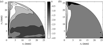
 ${\it\Pi}$
does nevertheless turn out to be fairly isotropic at
 $x/x_{\ast }^{peak}=0.57$
though not at
 $x/x_{\ast }^{peak}=0.44$
. It should be noted also that the values of
 ${\it\Pi}$
are negative at both locations
 $x/x_{\ast }^{peak}=0.44$
and 0.57 for all separations probed here and that they do not vary much with
 $\boldsymbol{r}$
at
 $x/x_{\ast }^{peak}=0.57$
. We are therefore presented with a situation at
 $x/x_{\ast }^{peak}=0.57$
where
 ${\it\Pi}$
is negative and approximately uniform in value across our separation vectors, a situation very similar to (1.5). Yet, as mentioned in the first paragraph of this section, (1.7) does not hold at our measurement stations.
The nonlinear energy transfer term normalised by the energy dissipation,
 ${\it\Pi}/{\it\epsilon}^{\ast }$
, at (a)
 $x/x_{\ast }^{peak}=0.44$
and (b)
 $x/x_{\ast }^{peak}=0.57$
.

The violation of (1.7) results from the combined forward and inverse cascades already mentioned. The negative values of
 ${\it\Pi}$
throughout our
 $\boldsymbol{r}$
plane result from nonlinear energy transfers from one orientation of
 $\boldsymbol{r}$
to another at constant
 $r=|\boldsymbol{r}|$
. This has to do with the topology of the interscale flux vector field in
 $\boldsymbol{r}$
space (see figures 16
a and 17
a). The seemingly attracting inverse cascade axis which lies at a small angle to the streamwise direction (see figures 16
a and 17
a) imposes a negative transfer in orientations (from
 ${\it\theta}={\rm\pi}/2$
to smaller) between this axis and the streamwise direction (where
 ${\it\Pi}_{r}>0$
) and a positive transfer in orientations (towards increasing angles
 ${\it\theta}$
) in the rest of the
 $\boldsymbol{r}$
plane (where
 ${\it\Pi}_{r}<0$
). As the circumferentially averaged transfer in orientations equals 0, i.e. as
 $\int _{0}^{{\rm\pi}/2}{\it\Pi}\,\text{d}{\it\theta}=\int _{0}^{{\rm\pi}/2}{\it\Pi}_{r}\,\text{d}{\it\theta}$
, and as the negative transfer in orientations (from
 ${\it\theta}={\rm\pi}/2$
to 0) is confined over a region in the
 $\boldsymbol{r}$
plane that is significantly smaller than the region where the transfer in orientations is positive (i.e. towards increasing angles
 ${\it\theta}$
), we can expect the negative values of
 ${\it\Pi}-{\it\Pi}_{r}$
(confined to the region where
 ${\it\Pi}_{r}>0$
) to be significantly larger in magnitude than the positive values of
 ${\it\Pi}-{\it\Pi}_{r}$
(in the rest of the
 $\boldsymbol{r}$
plane where
 ${\it\Pi}_{r}<0$
). These kinematic considerations explain why
 ${\it\Pi}$
can be negative throughout
 $\boldsymbol{r}$
, as indeed observed, but do not explain why it actually is negative at both
 $x/x_{\ast }^{peak}=0.44$
and 0.57 and approximately uniform in
 $\boldsymbol{r}$
at
 $x/x_{\ast }^{peak}=0.57$
.
We close this section with a summary of our findings so far.
-
(i) At our measurement stations in the production region around the centreline points
$x/x_{\ast }^{peak}=0.44$
(where
$\mathit{Re}_{{\it\lambda}}=190$
) and
$x/x_{\ast }^{peak}=0.57$
(where
$\mathit{Re}_{{\it\lambda}}\approx 270$
) the interscale energy transfers are characterised by a combination of an inverse cascade along an attracting axis at a small angle to the streamwise direction and a forward cascade in the transverse direction. For this reason there is no relation such as (1.7) valid at these production region points and there is no small-scale isotropy either. -
(ii) Nevertheless, there is a well-defined
$-5/3$
streamwise energy spectrum
$E_{11}(k_{1})$
, particularly at
$x/x_{\ast }^{peak}=0.57$
where
$\mathit{Re}_{{\it\lambda}}\approx 270$
. -
(iii) The directionally averaged cascade is forward, i.e. from large to small scales, and the
$r$
dependence of
$\overline{{\it\delta}u_{\Vert }{\it\delta}q^{2}}^{a}$
is not too far from
$\overline{{\it\delta}u_{\Vert }{\it\delta}q^{2}}^{a}=-16{\it\epsilon}r/9$
at
$x/x_{\ast }^{peak}=0.57$
. The coefficient
$16/9$
should not be given too much significance as it can be expected to be, at least residually, Reynolds-number dependent. -
(iv) Even without directional averages,
${\it\Pi}$
is negative at both
$x/x_{\ast }^{peak}=0.44$
and 0.57 and approximately uniform in
$\boldsymbol{r}$
at
$x/x_{\ast }^{peak}=0.57$
. This results from the combination of nonlinear transfers across separation scales and across separation orientations.





In the following section we show that the turbulence at these measurement stations is not homogeneous at the scales
 $r$
considered and that it is therefore not possible to reduce the inhomogeneous Kármán–Howarth (1.2) to the simpler form (1.3) which is typically used to derive the Richardson–Kolmogorov cascade and its consequences from Kolmogorov’s assumption of local equilibrium.
6. Energy transfer budget
6.1. Small and negligible terms
The energy transfer via the mean velocity gradients
 ${\it\Pi}_{U}$
, the viscous transport
 $\mathscr{D}_{X,{\it\nu}}^{\ast }$
and the viscous diffusion
 $\mathscr{D}_{{\it\nu}}^{\ast }$
are found to be small compared with the other terms in (1.2) that we can estimate and in particular small compared with
 ${\it\epsilon}^{\ast }$
.
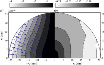
Figure 20(a) shows the flux vector
 $({\it\delta}U\overline{{\it\delta}q^{2}},0,0)~(\text{m}^{3}~\text{s}^{-3})$
(see the data reduction in § 4) and the isocontours of its magnitude
 $|{\it\delta}U\overline{{\it\delta}q^{2}}|$
, whereas figure 20(b) presents the divergence of this flux,
 ${\it\Pi}_{U}$
, which is normalised by
 ${\it\epsilon}^{\ast }$
. The divergence of
 ${\it\delta}U\overline{{\it\delta}q^{2}}$
takes maximum values at separations that have large
 $r_{1}$
and small
 $r_{3}$
values. These maximum values are of the order of
 $0.25{\it\epsilon}^{\ast }$
. For similar separations (
 $r_{1},r_{3}$
), the advection
 $\mathscr{A}$
takes on values close to
 $9{\it\epsilon}^{\ast }$
(see figure 22
a) and the turbulent transport
 $\mathscr{T}$
values close to
 $10{\it\epsilon}^{\ast }$
(see figure 22
b), which makes the divergence of
 ${\it\delta}U\overline{{\it\delta}q^{2}}$
negligible. In fact, as a cursory comparison of figures 20(b) and 22 rightly suggests,
 ${\it\Pi}_{U}$
is much smaller than both
 $\mathscr{A}$
and
 $\mathscr{T}$
at all
 $\boldsymbol{r}$
.
(a) The linear flux field
 $({\it\delta}U,0)\overline{{\it\delta}q^{2}}~(\text{m}^{3}~\text{s}^{-3})$
together with the isocontours of its magnitude
 $|{\it\delta}U\overline{{\it\delta}q^{2}}|~(\text{m}^{2}~\text{s}^{-2})$
. (b) Isocontours of
 ${\it\Pi}_{U}/{\it\epsilon}^{\ast }$
at
 $x/x_{\ast }^{peak}=0.44$
.

The viscous diffusion term,
 $\mathscr{D}_{X,{\it\nu}}$
, was estimated for
 $r_{3}=0$
and was found to be two orders of magnitude smaller than
 ${\it\epsilon}^{\ast }$
, irrespective of
 $r_{1}$
. It is therefore, as expected, not considered important for the Kármán–Howarth two-point energy budget.
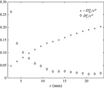
Figure 21 is a plot of the
 $r$
dependences of
 ${\it\Pi}_{U}^{a}=(2/{\rm\pi})\int _{0}^{{\rm\pi}/2}{\it\Pi}_{U}\,\text{d}{\it\theta}$
and
 $\mathscr{D}_{{\it\nu}}^{a}=(2/{\rm\pi})\int _{0}^{{\rm\pi}/2}\mathscr{D}_{{\it\nu}}\,\text{d}{\it\theta}$
normalised by
 ${\it\epsilon}^{a}=(2/{\rm\pi})\int _{0}^{{\rm\pi}/2}{\it\epsilon}^{\ast }\,\text{d}{\it\theta}$
. This figure shows that viscous diffusion tends to increase with decreasing
 $r$
, which agrees with the constraint that
 $\mathscr{D}_{{\it\nu}}$
tends to
 ${\it\epsilon}(\boldsymbol{X})$
as
 $r$
tends to 0. The maximum values of
 ${\it\Pi}_{U}^{a}+\mathscr{D}_{{\it\nu}}^{a}$
are below approximately 30 % of the energy dissipation, which is negligible when compared with the other terms estimated in § 6.2.
Circumferentially averaged energy transfer by the mean velocity gradients
 ${\it\Pi}_{U}^{a}$
and viscous diffusion
 $\mathscr{D}_{{\it\nu}}^{a}$
normalised by the circumferentially averaged energy dissipation
 ${\it\epsilon}^{a}$
at
 $x/x_{\ast }^{peak}=0.44$
.

(a) The advection term normalised by the energy dissipation,
 $\mathscr{A}/{\it\epsilon}^{\ast }$
, and (b) the turbulence transport normalised by the energy dissipation,
 $\mathscr{T}/{\it\epsilon}^{\ast }$
, at
 $x/x_{\ast }^{peak}=0.44$
.

6.2. Main terms
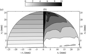
Figure 22 is a plot in
 $(r_{1},r_{3})$
space of the advection (
 $\mathscr{A}$
) and turbulent transport (
 $\mathscr{T}$
) terms normalised by the energy dissipation
 ${\it\epsilon}^{\ast }$
. Both terms are shown to be fairly isotropic in the sense that their contour lines resemble circles, at least up to the maximum radius considered here. In addition, given that their magnitudes are roughly similar particularly at the smaller scales, there seems to be a tendency for these two terms to cancel much (though not all) of each other in (1.2).
Figure 23 is also a plot in
 $(r_{1},r_{3})$
space but of the production (
 $\mathscr{P}$
) and the remainder
 $-\mathscr{B}$
of the Kármán–Howarth–Monin balance (1.2), both normalised by
 ${\it\epsilon}^{\ast }$
. Both of these terms are larger than the energy dissipation for transverse separations
 $r_{3}$
that are not too small. This is not surprising for the production term as, in the production region, the turbulence intensity and
 $\overline{{\it\delta}q^{2}}$
(see figure 15) increase with streamwise distance from the grid. Qualitatively, these terms behave differently compared with the advection and turbulent transport in figure 22. The main difference is that the contours appear stratified in figure 23 as opposed to circular in figure 22. The stratification of the production term in the
 $r_{3}$
direction (figure 23
a) is due to the mean velocity gradients being much larger in that direction than in the
 $r_{1}$
direction. This fact is patent in the mean velocity field, see figure 5(b).
(a) The production term normalised by the energy dissipation,
 $\mathscr{P}/{\it\epsilon}^{\ast }$
, and (b) the remainder of the Kármán–Howarth balance normalised by the energy dissipation,
 $-\mathscr{B}/{\it\epsilon}^{\ast }$
, at
 $x/x_{\ast }^{peak}=0.44$
.

Besides
 ${\it\Pi}$
and
 ${\it\epsilon}^{\ast }$
, the main terms in the Kármán–Howarth–Monin balance (1.2) at the location of the production region where we can estimate them (
 $x/x_{\ast }^{peak}=0.44$
) are
 $\mathscr{A}$
,
 $\mathscr{T}$
,
 $\mathscr{P}$
and
 $-\mathscr{B}$
. The approximate Kármán–Howarth–Monin balance that we are therefore faced with is
 $$\begin{eqnarray}{\it\Pi}\approx -{\it\epsilon}^{\ast }+\mathscr{P}+(\mathscr{T}-\mathscr{A})+\mathscr{B},\end{eqnarray}$$
where we might expect a significant part of
 $\mathscr{B}$
to be the pressure transport term
 $\mathscr{T}_{p}$
, see § 4. Laizet & Vassilicos (Reference Laizet and Vassilicos2012) reported that at a distance
 $x/x_{\ast }^{peak}=0.44$
from a turbulence-generating fractal grid similar to ours, the average pressure is still recovering. It is indeed reasonable to expect the pressure transport term
 $\mathscr{T}_{p}$
to be important in the production region.
In figure 24 we plot the terms in (6.1) at
 $x/x_{\ast }^{peak}=0.44$
but averaged over
 ${\it\theta}$
and normalised by
 ${\it\epsilon}^{a}=(2/{\rm\pi})\int _{0}^{{\rm\pi}/2}{\it\epsilon}^{\ast }\,\text{d}{\it\theta}$
. The production term
 $\mathscr{P}^{a}=(2/{\rm\pi})\int _{0}^{{\rm\pi}/2}\mathscr{P}\,\text{d}{\it\theta}$
is positive, meaning production of turbulence fluctuations by the mean flow, and is comparable to the nonlinear energy transfer
 $-{\it\Pi}^{a}=-(2/{\rm\pi})\int _{0}^{{\rm\pi}/2}{\it\Pi}\,\text{d}{\it\theta}$
. The terms of highest magnitude, however, are the advection
 $\mathscr{A}^{a}=(2/{\rm\pi})\int _{0}^{{\rm\pi}/2}\mathscr{A}\,\text{d}{\it\theta}$
and the turbulent transport
 $\mathscr{T}^{a}=(2/{\rm\pi})\int _{0}^{{\rm\pi}/2}\mathscr{T}\,\text{d}{\it\theta}$
, both positive, and the remainder
 $\mathscr{B}^{a}=(2/{\rm\pi})\int _{0}^{{\rm\pi}/2}\mathscr{B}\,\text{d}{\it\theta}$
which turns out to be negative. As already mentioned,
 ${\it\Pi}^{a}$
is negative, but also, perhaps remarkably, varies less with
 $r$
than all the other terms in (6.1). Combining expression (6.1) with (5.2) which follows from the near-constancy of
 ${\it\Pi}^{a}$
, we obtain
 $$\begin{eqnarray}\overline{{\it\delta}u_{\Vert }{\it\delta}q^{2}}^{a}\approx -{\textstyle \frac{4}{3}}r\left({\it\epsilon}^{a}-\mathscr{P}^{a}-(\mathscr{T}^{a}-\mathscr{A}^{a})-\mathscr{B}^{a}\right),\end{eqnarray}$$
which is similar to (1.7), in particular because
 ${\it\epsilon}^{a}-\mathscr{P}^{a}-(\mathscr{T}^{a}-\mathscr{A}^{a})-\mathscr{B}^{a}$
(which turns out to be approximately equal to
 $(4/3){\it\epsilon}^{a}$
here, see the paragraph under (5.2)) is only weakly dependent on
 $r$
, yet very different.
Circumferentially averaged nonlinear energy transfer (
 $-{\it\Pi}^{a}$
), advection (
 $-\mathscr{A}^{a}$
), production (
 $\mathscr{P}^{a}$
), turbulent transport (
 $\mathscr{T}^{a}$
) and remainder
 $\mathscr{B}^{a}$
normalised by the circumferentially averaged energy dissipation
 ${\it\epsilon}^{a}$
at
 $x/x_{\ast }^{peak}=0.44$
.

7. Conclusions
The focus of this work has been the two-point statistics of turbulence fluctuations in the most inhomogeneous and anisotropic region of grid-generated turbulence. This region is termed the production region and lies between the grid and the peak of turbulence intensity downstream of it. In order to magnify the space where PIV can be performed and to capture the smallest scales of the flow while maintaining a good dynamic range in space, we have used a well-documented turbulence-generating fractal square grid which is known to magnify the streamwise extent of the production region and abate its turbulence activity. We performed planar two-component PIV measurements of many terms of the non-homogeneous Kármán–Howarth–Monin equation in this region. We found the turbulence to be indeed significantly inhomogeneous and anisotropic even at scales smaller than the Taylor microscale around the centre of that region on the centreline. The two-point advection and transport terms are dominant and the production is significant also in the Kármán–Howarth–Monin balance. The importance of the two-point advection indicates that one cannot apply the local equilibrium hypothesis (1.4) of Kolmogorov. It is therefore impossible to apply usual Kolmogorov arguments based on the Kármán–Howarth–Monin equation and resulting dimensional considerations to deduce interscale flux and spectral properties.
We find that the interscale energy transfers are characterised by a combination of an inverse cascade along an attractive axis, which is at a small angle with the streamwise direction, and a forward cascade in the transverse direction. For this reason there is no relation such as (1.7), which requires a forward cascade for all separations, valid at our production region points, and there is no small-scale isotropy either. Even so, the energy spectrum of the streamwise fluctuating component exhibits a well-defined
 $-5/3$
power law over one decade.
The directionally averaged cascade is forward, i.e. from large to small scales, and the
 $r$
dependence of
 $\overline{{\it\delta}u_{\Vert }{\it\delta}q^{2}}^{a}$
is not too far from linear in
 $r$
at
 $x/x_{\ast }^{peak}=0.57$
. The directionally averaged nonlinear energy transfer term
 ${\it\Pi}^{a}$
is negative and varies less with
 $r$
than all the other terms in the approximate Kármán–Howarth–Monin balance (6.1).
Even without directional averages,
 ${\it\Pi}$
is negative at both
 $x/x_{\ast }^{peak}=0.44$
and 0.57 and approximately uniform in
 $\boldsymbol{r}$
at
 $x/x_{\ast }^{peak}=0.57$
. This results from the combination of nonlinear transfers across separation orientations as well as across scales.
It should be noted that power-law energy spectra with exponents close to
 $-5/3$
have also been reported in a cylinder wake within one cylinder diameter from the cylinder (Braza, Perrin & Hoarau Reference Braza, Perrin and Hoarau2006). It might be relevant to perform studies similar to ours in various very-near-field wakes and determine their interscale nonlinear cascade characteristics. In future works on near-field wakes and on the production region of grid-generated turbulence it will also be important to examine the assumptions that we were forced to make as a result of the 2D planar nature of our PIV. The first two main assumptions are stated at the end of the first paragraph of § 4 and the third main one is given in the same section and concerns our estimate of the divergence of the energy flux. The interpretations of the results in §§ 5 and 6 depend on these assumptions.
Acknowledgements
We gratefully acknowledge the financial support from EPSRC through grant no. EP/H030875/1.
Appendix A. Taylor’s hypothesis validation
The main results from the present paper assume that Taylor’s hypothesis is valid in the production region of the flow and are mainly focused at the location
 $x/x_{\ast }^{peak}=0.44$
. In order to assess the validity of this hypothesis at this station we present some indicators based on the SFV and the LFV.
The SFV is composed of
 $1280~\text{pixels}\times 64~\text{pixels}$
(see table 4) which translates into
 $80\times 3$
vectors, in the
 $z$
and
 $x$
directions respectively. The spatial derivatives (
 $\partial u/\partial x$
) are calculated using a second-order difference scheme with the first and third vectors in each row. The derivatives computed using Taylor’s hypothesis use the temporal information of the second vector and the following expression:
 $$\begin{eqnarray}\frac{\partial u^{d}(z)}{\partial x}=\frac{-1}{U(z)}\frac{\partial u(z)}{\partial t},\end{eqnarray}$$
where
 $U(z)$
is the mean velocity averaged through time information. Figure 25(a) shows the correlation coefficient between the aforementioned gradients along the
 $z$
direction in the centreline. In an attempt to improve the correlation, the convection velocity used in (A 1) (
 $U(z)$
) is computed using the local mean velocity (usual procedure when applying Taylor’s hypothesis) or using a local averaging window in the temporal data with different sizes, namely
 ${\it\lambda}/2$
(where
 ${\it\lambda}$
is the Taylor microscale),
 ${\it\lambda}$
,
 $L$
(
 $L$
is the integral length scale of
 $u$
in the
 $x$
direction) and 30
 $L$
. The use of local windows proved to capture better the derivative of strong events, but it is not as effective in capturing the weaker ones, resulting in a slight loss of the overall correlation. Nevertheless, the level of correlation is in line with what other authors have reported, such as Ganapathisubramani, Lakshminarasimhan & Clemens (Reference Ganapathisubramani, Lakshminarasimhan and Clemens2007) and Gomes-Fernandes et al. (Reference Gomes-Fernandes, Ganapathisubramani and Vassilicos2014), and Taylor’s hypothesis is applied using a global mean velocity as the convection velocity.
Validation of Taylor’s hypothesis at
 $x/x_{\ast }^{peak}=0.44$
: (a) correlation coefficient between
 $\partial u/\partial x$
and
 $\partial u^{d}/\partial x$
for several averaging window sizes and (b) second-order structure function calculated with spatial and temporal (by Taylor’s hypothesis) data.

Figure 25(b) shows the second-order structure function
 $\langle {\it\delta}u^{2}(r)\rangle$
at the centreline at
 $x/x_{\ast }^{peak}=0.44$
calculated using temporal data and Taylor’s hypothesis and spatial data. The spatial data are computed using the LFV which is
 $100~\text{mm}\times 180~\text{mm}$
and the statistics are converged with 5 runs of 8126 vector fields each. In the spatial data the centreline at
 $x/x_{\ast }^{peak}=0.44$
is kept as the centroid and
 $\langle {\it\delta}u^{2}(r)\rangle$
is computed between points equidistant from this point in the
 $x$
direction. The agreement between the two methods is good, which indicates that Taylor’s hypothesis is valid in this region.