Introduction
Simplicity, accuracy, and precision are the desired qualities of statistical estimators, and finding a balance of these properties has proven difficult with respect to measuring speciation and extinction rates. The recently proposed gap-filler (GF) equation (Alroy Reference Alroy2014) was intended to have these properties, but its precision is not very high. The purpose of this note is to introduce a heuristic improvement to the GF estimator that increases its precision and even its accuracy but is extremely simple. The GF equation's general properties are briefly restated below because readers may not be familiar with it.
To save space, no direct comparisons are made with older range-based equations such as those of Alroy (Reference Alroy1996) and Foote (Reference Foote1999, Reference Foote2000) and even older ones that were reviewed by Foote (Reference Foote1994). Such comparisons have already been made in detail (Alroy Reference Alroy2014), and the upshot is that these equations are often precise but have been argued to be biased by the Signor-Lipps, edge, Pull of the Recent effects, and by a taxonomic artifact related to the undersplitting of rare taxa. In other words, older equations suggest that extinction rates are elevated in intervals that precede mass extinctions but are not immediately before them; create gradual declines as the Recent is approached; and produce lower turnover rates for rare higher taxa, which is counterintuitive. The reason that older methods are biased in these ways is that they employ full age-ranges instead of examining patterns of sampling across limited temporal windows, which is the approach taken here and in related earlier studies (Alroy Reference Alroy2008, Reference Alroy2014).
Method
Moving-window methods (Alroy Reference Alroy2008, Reference Alroy2014) assume that there is a focal time interval (call it i 1) and that a cohort has been defined by only considering taxa sampled in the preceding one (i 0). Four categories of taxa have been discussed previously: those sampled in i 0 and i 1 (two-timers or t 2), those sampled in i 0, i 1, and i 2 (three-timers or t 3), those sampled in i 0 and i 2 but not in i 1 (part-timers or p), and those sampled in i 0 and i 3 but not in i 2 (gap-fillers or g). The three-timer (3T) and gap-filler (GF) equations use these counts and were respectively presented by Alroy (Reference Alroy2008) and Alroy (Reference Alroy2014). In this paper I put aside 3T because it has been shown to be much less precise than GF.
The GF equation for the instantaneous per interval extinction rate µ is the following log ratio:
 $${\mu }={\rm ln}\left[ {(t_{\it 2} {\plus}p)/(t_{\it 3} {\plus}p{\plus}g)} \right].$$
GF can be rearranged to yield an extinction proportion (i.e., the number of extinctions per taxon per interval) (Alroy Reference Alroy2014):
 $${\rm E}={\rm 1}{\minus}(t_{\it 3} {\plus}p{\plus}g)/(t_{\it 2} {\plus}p).$$
Another version is:
 $${\rm E}=(t_{\it 2} -t_{\it 3} -g)/(t_{\it 2} {\plus}p).$$
The new equation is best understood by reformulating equation (2) in yet another way. Let us first define two new categories: s 1=those taxa sampled in i 0 and i 1 but not later (first-interval taxa) and s 3=those sampled in i 0 and i 3 but not in i 1 or i 2 (third-interval taxa). The s 1 and s 3 patterns have both been illustrated previously (Alroy Reference Alroy2014: Fig. 2) but have not been the subject of any specific discussion.
Now assume that sampling is incomplete but uniform. When turnover is zero, one should expect s 1 to equal s 3. When turnover is very fast, s 3 should limit on zero. The difference s 1−s 3 should therefore be some function of the turnover rate. By careful inspection of Fig. 2 in Alroy (Reference Alroy2014), it will become apparent that s 1−s 3=t 2−t 3−g and therefore that:
 $${\rm E}=(s_{\it 1} -s_{\it 3} )/(t_{\it 2} {\plus}p).$$
The problem with this equation is that the four counts are often small, creating high amounts of random sampling error. I note in passing that there are two simple ways to decrease the variance by increasing the denominator. The first is to add in the very smallest count:
 $${\rm E}=(s_{\it 1} -s_{\it 3} )/(t_{\it 2} {\plus}p{\plus}s_{\it 3} ).$$
This metric performs well in simulations resembling those presented below and it could hardly be simpler. It does introduce an obvious downwards bias, but the amount of bias is small.
A second equation that can be shown by simulation to be similarly precise and more accurate is
 $${\rm E}=s_{\it 1} /(t_{\it 2} {\plus}p{\plus}s_{\it 3} )-s_{\it 3} /(t_{\it 2} {\plus}p{\plus}s_{\it 1} {\plus}s_{\it 2} ),$$
where s 2=the number of taxa sampled in i 0 and i 2 but not in i 1 or i 3 (one of two patterns producing the part-timer count p, just as s 1 is a subset of t 2 and s 3 is a subset of g).
Regardless of equation (6)'s merits, it is trumped in simulation by a very simple algorithmic approach. Consider the relations among the first-, second-, and third-interval taxa. Given that sampling is reasonably uniform albeit partial and that extinction is a one way street, the counts should have the order s 1≥s 2≥s 3. They often do not, either because the ordering is entirely reversed (s 1<s 2<s 3), s 2 is the minimum (s 2<s 1 and s 2<s 3), or s 2 is the maximum (s 2>s 1 and s 2>s 3). In such cases I propose substituting the second-lowest of the three counts for s 3 in equation (4). No further manipulation is necessary. In practice, this will mean doing nothing if s 3 is already in between s 1 and s 2; computing a zero rate if s 1 is in between the other two, which could happen if the GF rate is either negative or positive; and otherwise substituting s 2 for s 3, which can only happen if the GF rate is negative and which will edge the rate closer to zero.
I have been unable to find any other corrections that meet reasonable criteria (as detailed later) and substantially increase precision while generating only small amounts of bias. However, whether the improvement is worthwhile is really a practical matter. We will therefore move on to analyses of simulated and empirical data involving the new algorithm, which I call second-for-third substitution because the second-highest count is substituted for the third-interval taxon count.
Simulation Analyses
Figure 1A presents an example of a Monte Carlo simulation trial in which there are 50 time intervals; a fixed-size sampling pool of 100 taxa; a per-taxon, per-interval sampling probability p s of 0.3; and no turnover.
Two examples of 50-interval simulation trials. Parameters are described in the text. Thick lines=second-for-third proportions; thin lines=conventional gap-filler proportions (Alroy Reference Alroy2014). A, A simulation in which there is no actual turnover between intervals. B, A simulation in which there is 30% turnover.

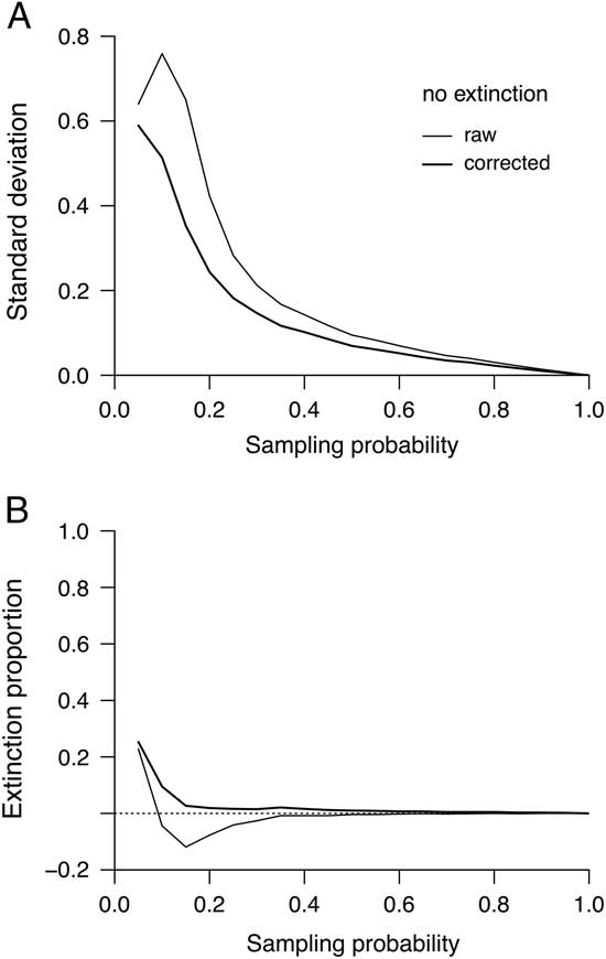
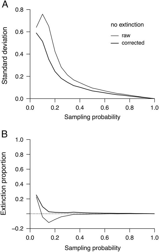
It is easy to see that the second-for-third correction primarily serves to ameliorate outlying negative values. This decrease in variance is also illustrated by trials in which there are 1000 intervals and the sampling probability is varied (Fig. 2A). Meanwhile, the corrected proportions are substantially biased only when sampling is very poor (Fig. 2B). In other words, even if sampling is as bad as p s=0.15 the algorithm generates no bias while very substantially increasing precision. By contrast, the raw GF proportions are just as upwards-biased when p s=0.05 but transiently downwards-biased at modest levels.
Results based on 1000-interval simulation trials in which the sampling probability is varied between 0.05 and 1 and there is no turnover. Thick and thin lines are as in Figure 1. A, Relationship between sampling probabilities and standard deviations of estimates across trials. B, Relationship between sampling probabilities and average estimated extinction proportions.
Similar results are seen (Figs. 1B, 3) when one imposes a probability of turnover at each interval boundary of 0.3 (this being here the chance that a taxon will be removed and immediately replaced with a new one). The difference in variance between the raw and corrected GF estimates is not as extreme but is still considerable (Fig. 3A). Meanwhile, there is now no large or consistent difference in accuracy (Fig. 3B).
Results based on 1000 interval simulation trials in which the sampling probability is varied between 0.05 and 1 and the per interval extinction proportion is always 0.3. Thick and thin lines are as in Fig. 1. A, Relationship between sampling probabilities and standard deviations of estimates across trials. B, Relationship between sampling probabilities and average estimated extinction proportions.

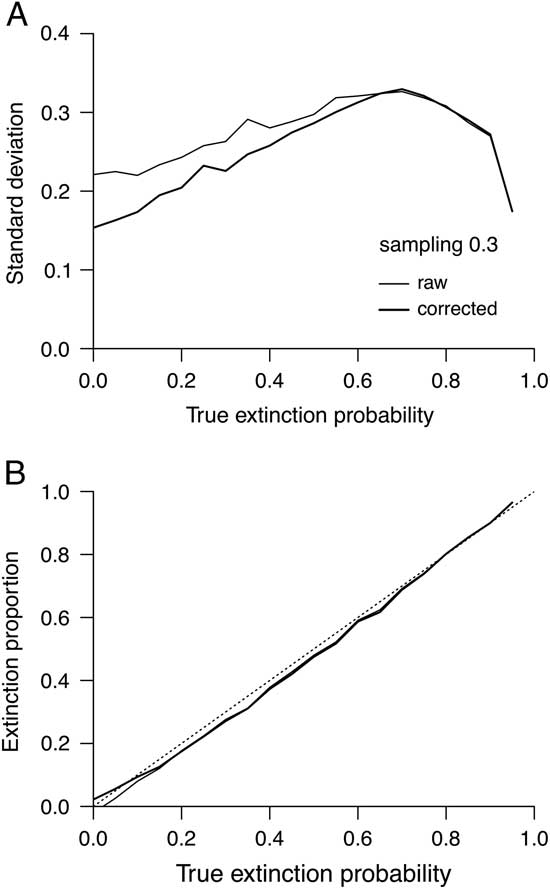
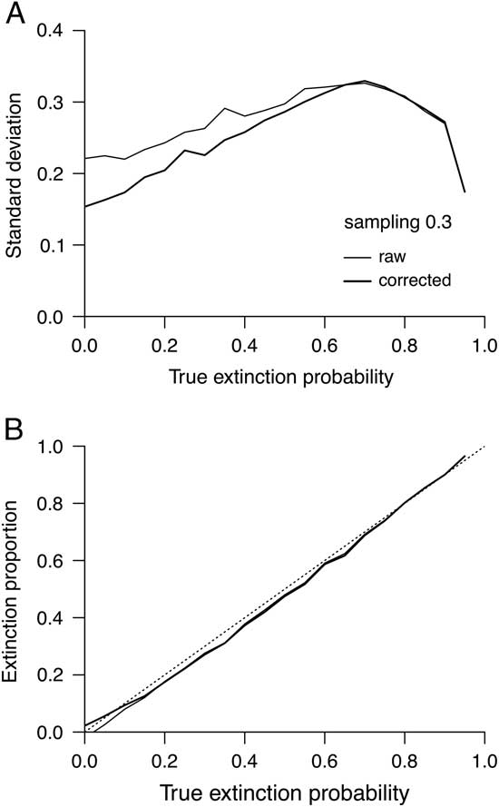
Finally, varying the turnover rate between 0 and 1 while holding p s to 0.3 demonstrates that the correction is helpful even at relatively good sampling levels of around p s=0.5 (Fig. 4A). It is also apparent that both equations are in most cases slightly downwards-biased (Fig. 4B). The reason is that trials have been excluded when t 2+p=0 because this sum is the denominator of equation (4). In all other cases, by definition the denominator is on average farther above zero than the true expected mean. The alternative of including such trials but assuming a proportion of 1 seems unreasonable given that it would mean the taxonomic group went entirely extinct over and over. The fact that the equations produce virtually the same expected values however fast turnover might be (Fig. 4B) while producing quite different amounts of variance (Fig. 4A) is actually more relevant.
Results based on 1000 interval simulation trials in which extinction proportions are varied but the sampling probability is always 0.3. Thick and thin lines are as in Figure 1. A, Relationship between assumed extinction proportions and standard deviations of estimates across trials. B, Relationship between assumed proportions and average estimated extinction proportions.
Analysis of Phanerozoic Marine Data
The problem of reducing error in rate estimates is of more than mere academic interest because the paleobiological literature is awash with studies of individual taxonomic groups whose fossil records are simply not that good. Small and variable sample sizes are seen even in data sets pertaining to major phyla and classes. However, obtaining reliable data for such groups is essential for such undertakings as defining evolutionary faunas (Sepkoski Reference Sepkoski1981), showing whether higher taxa replace each other deterministically (Gould and Calloway Reference Gould and Calloway1980), and looking for evidence of logistic dynamics (Miller and Sepkoski Reference Miller and Sepkoski1988).
The GF and second-for-third extinction rate curves are computed here for four of the very most major marine taxonomic groups (Anthozoa, Brachiopoda, Bivalvia, and Gastropoda) to show whether the choice of equations does matter. The data were downloaded using the Fossilworks portal to the Paleobiology Database on 23 October 2014 using standard vetting criteria and a time scale with ca. 10 Myr resolution that are described elsewhere (Alroy Reference Alroy2014). Contributors have been thanked previously. Raw counts were used instead of sampling-standardized counts to make the problem more challenging.
The four groups were selected because they are highly abundant and have good fossil records spanning the entire Ordovician to Quaternary interval. Thus, obtaining a long time series of precise rates should be easy. By contrast, groups such as ostracods, bryozoans, crinoids, and echinoids have erratically sampled records and others such as trilobites, graptolites, and conodonts went extinct too early to allow computing long time series. Cephalopods would also be worth examining, but are omitted here to save space.
In fact, the GF rates for the four groups are often negative even though they do capture obviously meaningful features such as peaks representing major mass extinctions (Fig. 5). Second-for-third substitution reduces the number of negative rates from five to four for Anthozoa, three to one for Brachiopoda, eight to five for Bivalvia, and 13 to six for Gastropoda. Of particular note, substitution ameliorates the pronounced outliers in all four data sets that correspond with the second Paleogene bin (equivalent to the Early Eocene). The effects are not helpful in every single case: for example, substitution creates two substantial wobbles in the Ordovician part of the Brachiopoda curve (Fig. 5B). Nonetheless, the general pattern is most fairly interpreted as a step in the right direction.
Genus level Phanerozoic extinction proportions for four major taxonomic groups. Thick and thin lines are as in Figure 1. A, Anthozoa. B, Brachiopoda. The truncated outlier in the Paleogene has a value of −0.714. C, Bivalvia. D, Gastropoda.

Putting aside subjective impressions, it would help to quantify the improvement in precision. One easy approach is to compute standard deviations of the proportions (instantaneous rates are not dealt with here because a few values would be infinite in cases where turnover is complete). The Anthozoa, Brachiopoda, Bivalvia, and Gastropoda standard deviations for the GF data are respectively 0.231, 0.289, 0.216, and 0.247. After substitution, the four statistics decline to 0.230, 0.256, 0.206, and 0.229. All of the pairs of standard deviations save the one for Anthozoa are significantly different at P<0.001 based on a bootstrap resampling analysis that involved randomly drawing the same number of rates from each time series with replacement and then computing the standard deviation. The procedure was iterated 1000 times and a paired Wilcoxon rank-sum test was performed to see if the resulting distributions differed.
Several interesting and important macroevolutionary patterns are visible in these curves. For example, the Anthozoa data suggest very high volatility that is consistent with the tendency of reefal organisms to suffer disproportionately during major mass extinctions (Kiessling and Simpson Reference Kiessling and Simpson2011). The Brachiopoda curve indicates persistently high background rates, a potential double pulse of extinction in the Late Permian, and an apparent shutdown in turnover in the latest Carboniferous and Early Permian that is highly peculiar. The Bivalvia curve depicts very low background rates punctuated by spikes that generally correspond to the major mass extinctions. And finally, the much more volatile Gastropoda curve agrees with it in suggesting that a fairly large extinction pulse might have characterized the Jurassic/Cretaceous boundary. All of these patterns are visible in the raw GF rates, but removing outliers and negative rates helps to cast them into clearer light.
In sum, the corrected GF equation produces figures that are still noisy—some negative rates are still present in all cases—but much more plausible. It stands to reason that similar noise reduction will be seen in other data sets, even in relatively large ones such as these.
Discussion
The new second-for-third algorithm is obviously heuristic. However, it meets a variety of sensible criteria for an estimator that corrects for sample size:
1. The procedure is so simple it can be computed by hand.
2. The GF equation's only clear-cut sources of information about the balance between extinction and sampling are the s 1 and s 3 counts (eq. 4). The correction involves the latter variable alone, so it avoids relying on counts such as t 2, p, and g that present mixed signals.
3. As mentioned, sampling error can cause s 1 to be less than s 3 even though there is no biological reason to ever see such a pattern. Suppose s 1 is zero and s 2<s 3. The rate will still be negative, but the correction will bring it closer to zero despite not generally creating a strong upwards bias in the estimator (as was shown previously). There is no a priori reason to employ a correction that might have the opposite effect.
4. Finally, the algorithm has good limit properties in the sense of only having an effect when sampling is poor, turnover rates are not high, and the species pool is modest. First, if sampling is perfect then s 2 and s 3 are zero and the counts therefore cannot be out of order, which means that no substitution is made. Second, if extinction is very rapid then the same thing is true because s 2 and s 3 both limit on zero. Third, if the number of taxa is very large then the ranking of s 1, s 2, and s 3 is very unlikely to be out of order, again making a correction unnecessary.
In sum, the worst-case scenario is that the algorithmically corrected version of GF might generate a small bias given very poor sampling (Figs. 2B, 3B). In many other circumstances it is likely to be highly accurate. We would expect no visible bias and substantially better accuracy given a realistic case in which a data set has fine stratigraphic resolution, which means that the extinction rate is well below 0.3, and in which p s is 0.1 to 0.5 (Figs. 2, 4). Furthermore, when sampling probabilities are clearly below 0.1 there are serious questions about whether turnover statistics should be computed in the first place.
Acknowledgments
I thank G. Hunt for a helpful review and A. Kocsis for raising my level of anxiety over the gap-filler equation's imprecision.