1 Introduction
Future aircraft turboengines will involve increased bypass ratios (BPR) to continue the trend of reducing fuel consumption,
 $\text{NO}_{x}$
and
 $\text{CO}_{2}$
emissions. Further noise reduction is also targeted with the new designs to ensure sustainable traffic growth with regards to increasing noise exposure. Ultra-high BPR (or UHBR) turboengines will have shorter nacelles to reduce both mass and drag. The acoustically treated area available in the inlet and exhaust portions of the UHBR nacelles will therefore be reduced, and the interstage region between the fan and the outlet guide vanes would then become more important for noise reduction. Yet, in the interstage region, the swirl induced by the fan is significant. Swirl can significantly modify the rotor wakes as they evolve toward the stator leading edges as predicted by Golubev & Atassi (Reference Golubev and Atassi2000a
) and observed experimentally by Podboy et al. (Reference Podboy, Krupar, Hughes and Woodward2002) for instance.
Furthermore, the types of disturbances that exist in the presence of swirl differ from those without swirl. They have been classified as upstream-going or downstream-going sonic modes, nearly convected modes and the non-modal continuous spectrum, also called the critical layer, and have been described in detail by Heaton & Peake (Reference Heaton and Peake2006). As a result, swirl will significantly modify the noise propagation as emphasised by Atassi et al. (Reference Atassi, Ali, Atassi and Vinogradov2004) and Cooper & Peake (Reference Cooper and Peake2005). Posson & Peake (Reference Posson and Peake2013a ) defined a new acoustic analogy and associated Green’s function in an annular duct with swirl which is a significant modification of the Green’s function without swirl, as illustrated by Posson & Peake (Reference Posson and Peake2013a ) and Mathews & Peake (Reference Mathews and Peake2017) both in hard wall and lined ducts. As a result, noise generated on rotor or stator blades and radiated in the interstage region is altered by the presence of swirl as highlighted by Golubev & Atassi (Reference Golubev and Atassi2000b ), Posson & Peake (Reference Posson and Peake2012), Posson & Peake (Reference Posson and Peake2013a ) and Masson et al. (Reference Masson, Posson, Sanjose, Moreau and Roger2016) for instance.
Another consequence of swirl is the modification of the liner response itself. When classical locally reacting liners are considered, a local impedance is usually defined to relate the acoustic pressure to the normal acoustic velocity at the liner surface. The impact of the flow on the liner impedance was first considered over fifty years ago. For instance Meyer, Mechel & Kurtze (Reference Meyer, Mechel and Kurtze1958) experimentally verified that the absorption of a liner was modified by a grazing flow. Ingard (Reference Ingard1959) proposed a boundary condition accounting for the continuity of the acoustic normal displacement at the liner surface, which considered the effect of mean flow parallel to the surface. Myers (Reference Myers1980) extended this result to any arbitrary mean flow along a curved wall. This Ingard–Myers impedance boundary condition has been extensively used for several decades. Yet, more recently, both experimentally and analytically, this Ingard–Myers boundary condition has been shown to have shortcomings. For instance, Renou & Aurégan (Reference Renou and Aurégan2010) could not retrieve consistent impedance values using the Ingard–Myers boundary condition from upstream- and downstream-propagating sound in experimental impedance eduction. Brambley (Reference Brambley2009) also suggested that the Ingard–Myers model was ill posed and had some inherent stability issues. Several extensions have been proposed since then that accounts for the presence of a boundary layer on top of the liner (Brambley Reference Brambley2011; Rienstra & Darau Reference Rienstra and Darau2011; Gabard Reference Gabard2013; Khamis & Brambley Reference Khamis and Brambley2016, Reference Khamis and Brambley2017). The effect of swirl was however not dealt with.
Particular emphasis in this study is put on the effect of swirl on the eigenmodes in an annular ducted flow with lined walls, accounting for the wall boundary layer at leading order. This could also be seen as an extension of the study by Posson & Peake (Reference Posson and Peake2013b ) to correct the use of the boundary condition to include swirl. Posson & Peake (Reference Posson and Peake2013a ) showed that nearly convected modes and the critical layer make negligible contributions to the pressure field in the hard wall case, although they will have to be considered in some specific cases where unstable hydrodynamic modes are predicted (Heaton & Peake Reference Heaton and Peake2006). As a result, they are not discussed here.
Finally, additional modes have been highlighted by Rienstra (Reference Rienstra2003) in a uniform flow besides the above three-dimensional acoustic duct modes. Indeed, at high frequencies and azimuthal order
 $m$
much smaller than the dimensionless frequency
 $\unicode[STIX]{x1D714}$
, he showed that up to four modes correspond to two-dimensional surface waves near the outer wall surface and that they are independent of the duct geometry. Their field decays exponentially away from the wall. Similarly, four modes correspond to surface waves at the inner wall. Brambley & Peake (Reference Brambley and Peake2006) generalised these results to arbitrary azimuthal mode order
 $m$
. The behaviour of the surface waves was also found to be dictated by a dimensionless parameter
 $\unicode[STIX]{x1D706}$
, termed the acoustic spinning parameter, that depends on
 $m$
,
 $\unicode[STIX]{x1D714}$
, the duct radius, the mean uniform axial velocity and the speed of sound. Brambley (Reference Brambley2013) then studied these surface waves in sheared boundary layers over liners. For a given frequency, up to six surface-wave modes were found at each wall, rather than the maximum of four per wall for uniform slipping flow. Their behaviour was not only dependent on the acoustic spinning parameter
 $\unicode[STIX]{x1D706}$
(using the centreline Mach number) but also on a dimensionless boundary-layer thickness and a boundary-layer shape factor. The importance of the boundary-layer thickness and profile was therefore demonstrated. Finally, different convective and absolute stability was also obtained in the sheared flow case. The present study will extend these results to the presence of swirl.
The governing equations are first presented in § 2. The correction to Myers’ boundary condition in the presence of a swirling flow is then derived to leading order in the boundary-layer thickness
 $\unicode[STIX]{x1D6FF}$
in § 3. Both the inner and outer solutions to the asymptotic problem are derived in §§ 3.3.1 and 3.3.2 respectively. They are then matched in § 3.3.3, which yields the boundary condition at both the inner duct wall and outer duct wall. In § 4 the new eigenvalue problem is formulated, and the effect of the new boundary condition is investigated on the eigenmodes. In § 5, the new set of eigenmodes are obtained and the influence of the new boundary condition on the acoustic propagation is studied. First, simpler cases are considered to validate the proper behaviour of the new boundary conditions. Then the actual turbofan model of the NASA Source Diagnostic Test (SDT) is considered to emphasise the impact of swirl in a realistic case. Finally, the surface waves in an annular duct with swirl are derived in § 6 and compared with the previous results of Brambley (Reference Brambley2013) in a simpler sheared flow.
2 Governing equations
The evolution of acoustic perturbations inside an inviscid compressible perfect gas is considered in an infinite annular duct with acoustic treatments both on the inner and the outer surfaces. The surface impedances of the inner and outer wall liners are
 $Z_{h}^{\ast }$
and
 $Z_{1}^{\ast }$
respectively. They are located at the radii
 $R_{h}^{\ast }$
and
 $R_{t}^{\ast }$
respectively, where the star
 $^{\ast }$
represents dimensioned coordinates. The mid-span radius is defined by
 $r_{m}^{\ast }=(R_{h}^{\ast }+R_{t}^{\ast })/2$
and
 $h=R_{h}^{\ast }/R_{t}^{\ast }$
is the hub-to-tip ratio. The duct section does not vary in the axial direction. Lengths, speeds and density are made dimensionless by
 $R_{t}^{\ast }$
, the dimensional speed of sound at mid-span
 $c_{0}^{\ast }(r_{m}^{\ast })$
and the mean density at mid-span
 $\unicode[STIX]{x1D70C}_{0}^{\ast }(r_{m}^{\ast })$
respectively, and other variables by the relevant combination of these values. The radial component of the mean flow is assumed to be zero and the axial and azimuthal components
 $U_{x}$
and
 $U_{\unicode[STIX]{x1D703}}$
may vary along the radius, leading to the following definition of the mean velocity field:
 $$\begin{eqnarray}\displaystyle & \displaystyle \boldsymbol{U}(r)=(0,U_{\unicode[STIX]{x1D703}}(r),U_{x}(r)). & \displaystyle\end{eqnarray}$$
The mean pressure
 $P_{0}$
satisfies the radial equilibrium
 $$\begin{eqnarray}\displaystyle & \displaystyle {\displaystyle \frac{\text{d}P_{0}}{\text{d}r}}=\unicode[STIX]{x1D70C}_{0}{\displaystyle \frac{U_{\unicode[STIX]{x1D703}}^{2}}{r}}. & \displaystyle\end{eqnarray}$$
The mean speed of sound
 $c_{0}$
and the mean density
 $\unicode[STIX]{x1D70C}_{0}$
may vary radially. Here a homentropic flow is considered, so that the sound speed and density are given by
 $$\begin{eqnarray}\displaystyle & \displaystyle c_{0}^{2}(r)=1+(\unicode[STIX]{x1D6FE}-1)\int _{r_{m}}^{r}{\displaystyle \frac{U_{\unicode[STIX]{x1D703}}^{2}(r^{\prime })}{r^{\prime }}}\,\text{d}r^{\prime }, & \displaystyle\end{eqnarray}$$
where
 $r_{m}=r_{m}^{\ast }/R_{t}^{\ast }$
, and
 $$\begin{eqnarray}\displaystyle & \displaystyle \unicode[STIX]{x1D70C}_{0}(r)=\left[c_{0}^{2}(r)\right]^{1/(\unicode[STIX]{x1D6FE}-1)}, & \displaystyle\end{eqnarray}$$
where
 $\unicode[STIX]{x1D6FE}$
is the ratio of specific heat capacities. Each flow variable (referred to with the subscript ‘
 $to$
’) is decomposed into a sum of a mean and a fluctuating part so that:
 $$\begin{eqnarray}\displaystyle \boldsymbol{U}_{to}=\boldsymbol{U}+\boldsymbol{u},\quad \unicode[STIX]{x1D70C}_{to}=\unicode[STIX]{x1D70C}_{0}+\unicode[STIX]{x1D70C},\quad P_{to}=P_{0}+p. & & \displaystyle\end{eqnarray}$$
Here,
 $\boldsymbol{u}=(u,v,w)$
, where
 $u$
,
 $v$
and
 $w$
are the radial, tangential and axial components of the fluctuating velocity respectively. The fluctuating pressure and density are given by
 $p$
and
 $\unicode[STIX]{x1D70C}$
respectively. The Euler equations linearised with respect to the mean flow defined in equations (2.1), (2.2), (2.3), (2.4) reduce to:
 $$\begin{eqnarray}\displaystyle & \displaystyle {\displaystyle \frac{1}{c_{0}^{2}}}{\displaystyle \frac{\text{D}_{0}p}{\text{D}t}}+u{\displaystyle \frac{\text{d}\unicode[STIX]{x1D70C}_{0}}{\text{d}r}}+\unicode[STIX]{x1D70C}_{0}\,\text{div}(\boldsymbol{u})=0, & \displaystyle\end{eqnarray}$$
 $$\begin{eqnarray}\displaystyle & \displaystyle \unicode[STIX]{x1D70C}_{0}\left[{\displaystyle \frac{\text{D}_{0}u}{\text{D}t}}-2{\displaystyle \frac{U_{\unicode[STIX]{x1D703}}v}{r}}\right]-{\displaystyle \frac{U_{\unicode[STIX]{x1D703}}^{2}}{rc_{0}^{2}}}p+{\displaystyle \frac{\unicode[STIX]{x2202}p}{\unicode[STIX]{x2202}r}}=0, & \displaystyle\end{eqnarray}$$
 $$\begin{eqnarray}\displaystyle & \displaystyle \unicode[STIX]{x1D70C}_{0}\left[{\displaystyle \frac{\text{D}_{0}v}{\text{D}t}}+{\displaystyle \frac{u}{r}}{\displaystyle \frac{\text{d}(rU_{\unicode[STIX]{x1D703}})}{\text{d}r}}\right]+{\displaystyle \frac{1}{r}}{\displaystyle \frac{\unicode[STIX]{x2202}p}{\unicode[STIX]{x2202}\unicode[STIX]{x1D703}}}=0, & \displaystyle\end{eqnarray}$$
 $$\begin{eqnarray}\displaystyle & \displaystyle \unicode[STIX]{x1D70C}_{0}\left[{\displaystyle \frac{\text{D}_{0}w}{\text{D}t}}+u{\displaystyle \frac{\text{d}U_{x}}{\text{d}r}}\right]+{\displaystyle \frac{\unicode[STIX]{x2202}p}{\unicode[STIX]{x2202}x}}=0, & \displaystyle\end{eqnarray}$$
 $\text{D}_{0}/\text{D}t$
is the convective operator with respect to the mean flow defined by
 $$\begin{eqnarray}\displaystyle & \displaystyle {\displaystyle \frac{\text{D}_{0}}{\text{D}t}}={\displaystyle \frac{\unicode[STIX]{x2202}}{\unicode[STIX]{x2202}t}}+U_{x}{\displaystyle \frac{\unicode[STIX]{x2202}}{\unicode[STIX]{x2202}x}}+{\displaystyle \frac{U_{\unicode[STIX]{x1D703}}}{r}}{\displaystyle \frac{\unicode[STIX]{x2202}}{\unicode[STIX]{x2202}\unicode[STIX]{x1D703}}}. & \displaystyle\end{eqnarray}$$
The pressure and velocity disturbances are Fourier transformed with respect to the time
 $t$
and the axial coordinate
 $x$
. Additionally, the azimuthal periodicity allows decomposing of the perturbation field as a Fourier series in the circumferential coordinate, allowing every acoustic variable to be written as:
 $$\begin{eqnarray}\displaystyle & \displaystyle \unicode[STIX]{x1D711}(r,\unicode[STIX]{x1D703},x,t)=\int _{\unicode[STIX]{x1D714}}\mathop{\sum }_{m\in \mathbb{Z}}\int _{k}\widehat{\unicode[STIX]{x1D711}}(r)\text{e}^{\text{i}(kx+m\unicode[STIX]{x1D703}-\unicode[STIX]{x1D714}t)}\,\text{d}k\,\text{d}\unicode[STIX]{x1D714}, & \displaystyle\end{eqnarray}$$
where
 $\widehat{\unicode[STIX]{x1D711}}$
is the Fourier transform of
 $\unicode[STIX]{x1D711}$
(
 $\unicode[STIX]{x1D711}$
standing for
 $p$
,
 $\unicode[STIX]{x1D70C}$
,
 $u$
,
 $v$
or
 $w$
),
 $\unicode[STIX]{x1D714}$
is the frequency,
 $k$
is the axial wavenumber and
 $m$
is the azimuthal mode order. Given
 $\unicode[STIX]{x1D6EC}=kU_{x}+mU_{\unicode[STIX]{x1D703}}/r-\unicode[STIX]{x1D714}$
, the linear governing equations in the spectral domain read:
 $$\begin{eqnarray}\displaystyle & \displaystyle \text{i}{\displaystyle \frac{\unicode[STIX]{x1D6EC}}{c_{0}^{2}}}\hat{p}=-{\displaystyle \frac{\text{d}\unicode[STIX]{x1D70C}_{0}}{\text{d}r}}\hat{u} -{\displaystyle \frac{\unicode[STIX]{x1D70C}_{0}}{r}}{\displaystyle \frac{\text{d}(r\hat{u} )}{\text{d}r}}-\text{i}{\displaystyle \frac{\unicode[STIX]{x1D70C}_{0}m}{r}}\hat{v}-\text{i}k\unicode[STIX]{x1D70C}_{0}{\hat{w}}, & \displaystyle\end{eqnarray}$$
 $$\begin{eqnarray}\displaystyle & \displaystyle \text{i}\unicode[STIX]{x1D70C}_{0}\unicode[STIX]{x1D6EC}\hat{u} =2{\displaystyle \frac{\unicode[STIX]{x1D70C}_{0}U_{\unicode[STIX]{x1D703}}}{r}}\hat{v}+{\displaystyle \frac{U_{\unicode[STIX]{x1D703}}^{2}}{rc_{0}^{2}}}\hat{p}-{\displaystyle \frac{\text{d}\hat{p}}{\text{d}r}}, & \displaystyle\end{eqnarray}$$
 $$\begin{eqnarray}\displaystyle & \displaystyle \text{i}\unicode[STIX]{x1D70C}_{0}\unicode[STIX]{x1D6EC}\hat{v}=-{\displaystyle \frac{\unicode[STIX]{x1D70C}_{0}}{r}}{\displaystyle \frac{\text{d}(rU_{\unicode[STIX]{x1D703}})}{\text{d}r}}\hat{u} -{\displaystyle \frac{\text{i}m}{r}}\hat{p}, & \displaystyle\end{eqnarray}$$
 $$\begin{eqnarray}\displaystyle & \displaystyle \text{i}\unicode[STIX]{x1D70C}_{0}\unicode[STIX]{x1D6EC}{\hat{w}}=-\unicode[STIX]{x1D70C}_{0}{\displaystyle \frac{\text{d}U_{x}}{\text{d}r}}\hat{u} -\text{i}k\hat{p}. & \displaystyle\end{eqnarray}$$
Using the radial equilibrium of the mean flow, these equations can be combined to yield a system of two coupled first-order differential equations on the pressure
 $\hat{p}$
and the radial fluctuating normal velocity
 $\hat{u}$
only. The first of these is given by
 $$\begin{eqnarray}\displaystyle & & \displaystyle \displaystyle {\displaystyle \frac{\text{d}\hat{u} }{\text{d}r}}+\left[{\displaystyle \frac{1}{r}}+{\displaystyle \frac{U_{\unicode[STIX]{x1D703}}^{2}(r)}{rc_{0}^{2}(r)}}-{\displaystyle \frac{k}{\unicode[STIX]{x1D6EC}(r)}}{\displaystyle \frac{\text{d}U_{x}(r)}{\text{d}r}}-{\displaystyle \frac{m}{\unicode[STIX]{x1D6EC}(r)r^{2}}}{\displaystyle \frac{\text{d}}{\text{d}r}}\left(rU_{\unicode[STIX]{x1D703}}(r)\right)\right]\hat{u} \nonumber\\ \displaystyle & & \displaystyle \quad +\,\text{i}{\displaystyle \frac{1}{\unicode[STIX]{x1D70C}_{0}(r)\unicode[STIX]{x1D6EC}(r)}}\left({\displaystyle \frac{\unicode[STIX]{x1D6EC}^{2}(r)}{c_{0}^{2}(r)}}-{\displaystyle \frac{m^{2}}{r^{2}}}-k^{2}\right)\hat{p}=0,\end{eqnarray}$$
which may be written equivalently:
 $$\begin{eqnarray}\displaystyle & \displaystyle {\displaystyle \frac{\text{d}}{\text{d}r}}\left({\displaystyle \frac{r\hat{u} }{\unicode[STIX]{x1D6EC}(r)}}\right)-{\displaystyle \frac{1}{\unicode[STIX]{x1D6EC}(r)}}\left({\displaystyle \frac{2mU_{\unicode[STIX]{x1D703}}(r)}{r\unicode[STIX]{x1D6EC}(r)}}-{\displaystyle \frac{U_{\unicode[STIX]{x1D703}}^{2}(r)}{c_{0}^{2}(r)}}\right)\hat{u} =-\text{i}{\displaystyle \frac{r}{\unicode[STIX]{x1D70C}_{0}(r)\unicode[STIX]{x1D6EC}^{2}(r)}}\left({\displaystyle \frac{\unicode[STIX]{x1D6EC}^{2}(r)}{c_{0}^{2}(r)}}-{\displaystyle \frac{m^{2}}{r^{2}}}-k^{2}\right)\hat{p}. & \displaystyle \nonumber\\ \displaystyle & & \displaystyle\end{eqnarray}$$
For the other equation, the radial-momentum linear equation (2.9b ) is rewritten:
 $$\begin{eqnarray}\displaystyle & \displaystyle {\displaystyle \frac{\text{d}\hat{p}}{\text{d}r}}+\left({\displaystyle \frac{2mU_{\unicode[STIX]{x1D703}}(r)}{\unicode[STIX]{x1D6EC}(r)r^{2}}}-{\displaystyle \frac{U_{\unicode[STIX]{x1D703}}^{2}(r)}{rc_{0}^{2}(r)}}\right)\hat{p}=-\text{i}{\displaystyle \frac{\unicode[STIX]{x1D70C}_{0}(r)}{\unicode[STIX]{x1D6EC}(r)}}\left(\unicode[STIX]{x1D6EC}^{2}(r)-{\displaystyle \frac{2U_{\unicode[STIX]{x1D703}}(r)}{r^{2}}}{\displaystyle \frac{\text{d}}{\text{d}r}}(rU_{\unicode[STIX]{x1D703}}(r))\right)\hat{u} . & \displaystyle\end{eqnarray}$$
Equations (2.10) and (2.12) are the equivalent of equations (A4) and (A7) in the appendices of Posson & Peake (Reference Posson and Peake2013a ) in the frequency domain. They are also the extension of Khamis & Brambley (Reference Khamis and Brambley2016, equation (2.10)) to a swirling flow. They will be used to establish the corrected Myers boundary condition.
3 Correction of Myers’ boundary condition in the presence of a swirling flow
Using the impedance definition as a boundary condition at the duct walls:
 $$\begin{eqnarray}\displaystyle \hat{p}(h)=-Z_{h}\hat{u} (h)\quad \text{and}\quad \hat{p}(1)=Z_{1}\hat{u} (1), & & \displaystyle\end{eqnarray}$$
would require properly accounting for the flow field near the wall to ensure a zero mean velocity on the wall. To avoid this complexity, it is convenient to consider a mean flow without boundary layers and to introduce instead an equivalent boundary condition that would mimic the real physical behaviour.
3.1 Classical Myers boundary condition
Assuming the continuity of the acoustic normal displacement through an infinitely thin boundary layer leads to the classical Ingard–Myers boundary condition (Ingard Reference Ingard1959; Myers Reference Myers1980). It reads with the present conventions:
 $$\begin{eqnarray}\displaystyle \hat{u} (h)={\displaystyle \frac{kU_{x}(h)+mU_{\unicode[STIX]{x1D703}}(h)/h-\unicode[STIX]{x1D714}}{\unicode[STIX]{x1D714}Z_{h}}}\hat{p}(h),\quad \text{and}\quad \hat{u} (1)=-{\displaystyle \frac{kU_{x}(1)+mU_{\unicode[STIX]{x1D703}}(1)-\unicode[STIX]{x1D714}}{\unicode[STIX]{x1D714}Z_{1}}}\hat{p}(1), & & \displaystyle \nonumber\\ \displaystyle & & \displaystyle\end{eqnarray}$$
at the hub and at the tip respectively. In the following, it will be shown that (3.2) is not the correct limit when the boundary-layer thickness tends to zero in the presence of swirl.
3.2 Assumptions
The aim of this section is to substitute the effect of a flow including a boundary layer with the boundary condition in (3.1) by an equivalent boundary condition in a flow where the boundary layer is not taken into account. In order to address such a problem, Eversman & Beckemeyer (Reference Eversman and Beckemeyer1972) proposed an approach based on an asymptotic matching between an inner solution in the boundary layer, and an outer solution outside the boundary layer which would exist if there was no boundary layer. This method has been reused by several authors such as Myers & Chuang (Reference Myers and Chuang1984), Brambley (Reference Brambley2011) and Khamis & Brambley (Reference Khamis and Brambley2016) for uniform axial flow. It is extended here to the case of a swirling flow. Considering a thin boundary layer at the wall (
 $r=1$
or
 $r=h$
) of typical width (in dimensional terms,
 $\unicode[STIX]{x1D6FF}^{\ast }$
should be smaller than any other length scale, including not only the mid-span radius
 $r_{m}^{\ast }$
but also axial and radial wavelengths. This will be noted where pertinent)
 $\unicode[STIX]{x1D6FF}$
,
 $\unicode[STIX]{x1D6FF}\ll 1$
, the distance to the wall
 $\unicode[STIX]{x1D6FF}y$
is introduced to develop the asymptotic expansion. As in Brambley (Reference Brambley2011), it is scaled by the boundary-layer thickness
 $\unicode[STIX]{x1D6FF}$
such that
 $r=1-\unicode[STIX]{x1D6FF}y$
at the outer wall and
 $r=h+\unicode[STIX]{x1D6FF}y$
at the inner wall. Let
 $U_{x}^{nbl}(r)$
and
 $U_{\unicode[STIX]{x1D703}}^{nbl}(r)$
be the outer mean flow velocity profiles without the boundary layer.
In the vicinity of walls, a Taylor expansion to first order applied on the outer mean flow velocity profiles reads:
 $$\begin{eqnarray}\displaystyle U_{x}^{nbl}(1-\unicode[STIX]{x1D6FF}y)=U_{x}^{nbl}(1)+O(\unicode[STIX]{x1D6FF}),\quad U_{\unicode[STIX]{x1D703}}^{nbl}(1-\unicode[STIX]{x1D6FF}y)=U_{\unicode[STIX]{x1D703}}^{nbl}(1)+O(\unicode[STIX]{x1D6FF}), & & \displaystyle\end{eqnarray}$$
 $$\begin{eqnarray}\displaystyle U_{x}^{nbl}(h+\unicode[STIX]{x1D6FF}y)=U_{x}^{nbl}(h)+O(\unicode[STIX]{x1D6FF}),\quad U_{\unicode[STIX]{x1D703}}^{nbl}(h+\unicode[STIX]{x1D6FF}y)=U_{\unicode[STIX]{x1D703}}^{nbl}(h)+O(\unicode[STIX]{x1D6FF}). & & \displaystyle\end{eqnarray}$$
Next, the outer mean flow is assumed constant up to leading order in the vicinity of the walls. For the sake of conciseness, the constants
 $M_{x,i}=U_{x}^{nbl}(i)$
and
 $M_{\unicode[STIX]{x1D703},i}=U_{\unicode[STIX]{x1D703}}^{nbl}(i)$
are introduced for
 $i=h,1$
. This assumption will be relaxed in § 3.5.
3.3 Derivation of the corrected boundary condition at the outer wall
The boundary condition is developed at the outer wall first.
3.3.1 Outer solution
The outer solution corresponds to the fluctuations propagating in the outer flow. The inner expansions of the outer solutions are obtained by writing a Taylor expansion of
 $\hat{u}$
and
 $\hat{p}$
in the vicinity of the outer wall. At leading order, it reads:
 $$\begin{eqnarray}\displaystyle & \displaystyle \hat{u} _{o}(1-\unicode[STIX]{x1D6FF}y)=\hat{u} _{o}(1)+O\left(\unicode[STIX]{x1D6FF}\right), & \displaystyle\end{eqnarray}$$
 $$\begin{eqnarray}\displaystyle & \displaystyle \hat{p}_{o}(1-\unicode[STIX]{x1D6FF}y)=\hat{p}_{o}(1)+O\left(\unicode[STIX]{x1D6FF}\right), & \displaystyle\end{eqnarray}$$
where the subscript
 $o$
stands for the outer solution. The eigenfunctions
 $\hat{p}_{o}$
and
 $\hat{u} _{o}$
represent the pressure and the radial velocity respectively if the boundary layer did not exist. Even if there is no analytic expression for them, they can be determined by a pseudo-spectral method for example, as done in § 4. They are assumed to be known, in particular
 $\hat{p}_{\infty }^{1}$
and
 $\hat{u} _{\infty }^{1}$
are introduced with
 $$\begin{eqnarray}\displaystyle & \displaystyle \hat{p}_{o}(1)=\hat{p}_{\infty }^{1},\quad \hat{u} _{o}(1)=\hat{u} _{\infty }^{1}. & \displaystyle\end{eqnarray}$$
In the following, the inner solution for
 $\hat{u}$
and
 $\hat{p}$
will be matched to (3.5) and (3.6).
3.3.2 Inner solution
To compute the inner solution, equations (2.11) and (2.12) are expanded by replacing
 $r$
by
 $1-\unicode[STIX]{x1D6FF}y$
. It is also possible to start the matching method from (2.9d
). To leading order, equation (2.12) becomes
 $$\begin{eqnarray}\displaystyle \hat{p}_{y}(y)={\displaystyle \frac{2\text{i}\unicode[STIX]{x1D70C}_{0}U_{\unicode[STIX]{x1D703}}U_{\unicode[STIX]{x1D703},y}}{kU_{x}+mU_{\unicode[STIX]{x1D703}}-\unicode[STIX]{x1D714}}}\hat{u} (y)+O(\unicode[STIX]{x1D6FF}), & & \displaystyle\end{eqnarray}$$
where the
 $y$
-dependence has been kept implicitly. The subscript
 $y$
represents the derivative with respect to
 $y$
and for every variable
 $\unicode[STIX]{x1D6F7}$
;
 $\unicode[STIX]{x1D6F7}(y)$
improperly stands for
 $\unicode[STIX]{x1D6F7}(r=1-\unicode[STIX]{x1D6FF}y)$
. Similarly, equation (2.11) is rewritten in terms of the inner variable
 $y$
 $$\begin{eqnarray}\displaystyle & \displaystyle \left({\displaystyle \frac{\hat{u} (y)}{kU_{x}+mU_{\unicode[STIX]{x1D703}}-\unicode[STIX]{x1D714}}}\right)_{y}=O\left(\unicode[STIX]{x1D6FF}\right). & \displaystyle\end{eqnarray}$$
The solution to these equations must be determined to be matched with the outer solution. The acoustic pressure and normal velocity are now considered as perturbation series, although only the leading-order term is required for our analysis:
 $$\begin{eqnarray}\displaystyle & \displaystyle \hat{p}(y)=\hat{p}_{0}(y)+O(\unicode[STIX]{x1D6FF}), & \displaystyle\end{eqnarray}$$
 $$\begin{eqnarray}\displaystyle & \displaystyle \hat{u} (y)=\hat{u} _{0}(y)+O(\unicode[STIX]{x1D6FF}). & \displaystyle\end{eqnarray}$$
The form of equation (3.9) allows determining of
 $\hat{u} _{0}$
. At zeroth order, it reduces to:
 $$\begin{eqnarray}\displaystyle & \displaystyle \left({\displaystyle \frac{\hat{u} _{0}(y)}{kU_{x}(y)+mU_{\unicode[STIX]{x1D703}}(y)-\unicode[STIX]{x1D714}}}\right)_{y}=0. & \displaystyle\end{eqnarray}$$
Then, by posing
 $\unicode[STIX]{x1D6EC}_{0}(y)=kU_{x}(y)+mU_{\unicode[STIX]{x1D703}}(y)-\unicode[STIX]{x1D714}$
,
 $$\begin{eqnarray}\displaystyle \hat{u} _{0}(y)=B_{0}\unicode[STIX]{x1D6EC}_{0}(y). & & \displaystyle\end{eqnarray}$$
Similarly, only leading-order terms in
 $\unicode[STIX]{x1D6FF}$
are kept in (3.8). This reads:
 $$\begin{eqnarray}\displaystyle & \displaystyle \hat{p}_{0,y}(y)={\displaystyle \frac{2\text{i}\unicode[STIX]{x1D70C}_{0}U_{\unicode[STIX]{x1D703}}(y)U_{\unicode[STIX]{x1D703},y}(y)}{\unicode[STIX]{x1D6EC}_{0}(y)}}\hat{u} _{0}(y), & \displaystyle\end{eqnarray}$$
and hence
 $$\begin{eqnarray}\displaystyle & \displaystyle \hat{p}_{0}(y)=A_{0}+\text{i}B_{0}\int _{0}^{y}\unicode[STIX]{x1D70C}_{0}(y^{\prime })\left(U_{\unicode[STIX]{x1D703}}^{2}(y^{\prime })\right)_{y^{\prime }}\,\text{d}y^{\prime }. & \displaystyle\end{eqnarray}$$
The integral term is bounded as
 $y\rightarrow \infty$
since
 $U_{\unicode[STIX]{x1D703}}(y)=M_{\unicode[STIX]{x1D703}}$
is assumed constant outside the boundary layer, and hence its derivative is zero. The constants
 $B_{0}$
and
 $A_{0}$
can be determined by matching the leading-order inner solutions with the outer ones.
3.3.3 Matching
Matching equation (3.13) with the outer solution (3.5) for large
 $y$
gives the value of the constant
 $B_{0}$
:
 $$\begin{eqnarray}\displaystyle B_{0}={\displaystyle \frac{\hat{u} _{\infty }^{1}}{\unicode[STIX]{x1D6EC}_{\infty }^{1}}}, & & \displaystyle\end{eqnarray}$$
where
 $\unicode[STIX]{x1D6EC}_{\infty }^{1}=kM_{x,1}+mM_{\unicode[STIX]{x1D703},1}-\unicode[STIX]{x1D714}$
has been defined for conciseness. Matching
 $\hat{p}_{0}$
defined in (3.15) with
 $\hat{p}_{o}$
in (3.6) for large
 $y$
gives:
 $$\begin{eqnarray}\displaystyle & \displaystyle A_{0}=\hat{p}_{\infty }^{1}-{\displaystyle \frac{\text{i}\hat{u} _{\infty }^{1}I_{0}}{\unicode[STIX]{x1D6EC}_{\infty }^{1}}}, & \displaystyle\end{eqnarray}$$
where
 $$\begin{eqnarray}\displaystyle & \displaystyle I_{0}=\int _{0}^{\infty }\unicode[STIX]{x1D70C}_{0}(y)\left(U_{\unicode[STIX]{x1D703}}^{2}(y)\right)_{y}\text{d}y=-\int _{r_{m}}^{1}\unicode[STIX]{x1D70C}_{0}(r){\displaystyle \frac{\text{d}}{\text{d}r}}\left(U_{\unicode[STIX]{x1D703}}^{2}(r)\right)\text{d}r. & \displaystyle\end{eqnarray}$$
3.3.4 Boundary condition
At
 $r=1$
(or
 $y=0$
), the surface impedance of the liner at the outer wall is defined by
 $Z_{1}=\hat{p}(1)/\hat{u} (1)$
. Furthermore, we note that
 $\unicode[STIX]{x1D6EC}_{0}(1)=-\unicode[STIX]{x1D714}$
since
 $U_{x}(1)=U_{\unicode[STIX]{x1D703}}(1)=0$
. As in Khamis & Brambley (Reference Khamis and Brambley2016), the boundary condition is expressed as an equivalent impedance relating
 $\hat{u} _{\infty }^{1}$
and
 $\hat{p}_{\infty }^{1}$
. At leading order, it reads:
 $$\begin{eqnarray}\displaystyle Z_{eff}^{\dagger }(1)={\displaystyle \frac{\hat{p}_{\infty }^{1}}{\hat{u} _{\infty }^{1}}}=-{\displaystyle \frac{\unicode[STIX]{x1D714}}{\unicode[STIX]{x1D6EC}_{\infty }^{1}}}Z_{1}^{\dagger }, & & \displaystyle\end{eqnarray}$$
 $$\begin{eqnarray}\displaystyle \text{with}~Z_{1}^{\dagger }=Z_{1}+{\displaystyle \frac{\text{i}}{\unicode[STIX]{x1D714}}}\int _{r_{m}}^{1}\unicode[STIX]{x1D70C}_{0}{\displaystyle \frac{\text{d}}{\text{d}r}}\left(U_{\unicode[STIX]{x1D703}}^{2}\right)\text{d}r, & & \displaystyle\end{eqnarray}$$
3.4 Extension to the inner wall
At the inner wall, the surface impedance is defined by
 $Z_{h}=-\hat{p}(h)/\hat{u} (h)$
. Applying the same method leads to the corrected Myers boundary condition at the inner wall:
 $$\begin{eqnarray}\displaystyle Z_{eff}^{\dagger }(h)=-{\displaystyle \frac{\hat{p}_{\infty }^{h}}{\hat{u} _{\infty }^{h}}}=-{\displaystyle \frac{\unicode[STIX]{x1D714}}{\unicode[STIX]{x1D6EC}_{\infty }^{h}}}Z_{h}^{\dagger }, & & \displaystyle\end{eqnarray}$$
 $$\begin{eqnarray}\displaystyle \text{with}~Z_{h}^{\dagger }=Z_{h}+{\displaystyle \frac{\text{i}}{h\unicode[STIX]{x1D714}}}\int _{h}^{r_{m}}\unicode[STIX]{x1D70C}_{0}{\displaystyle \frac{\text{d}}{\text{d}r}}\left(U_{\unicode[STIX]{x1D703}}^{2}\right)\text{d}r, & & \displaystyle\end{eqnarray}$$
 $\hat{p}_{\infty }^{h}=\hat{p}_{o}(h)$
,
 $\hat{u} _{\infty }^{h}=\hat{u} _{o}(h)$
and
 $\unicode[STIX]{x1D6EC}_{\infty }^{h}=kM_{x,h}+mM_{\unicode[STIX]{x1D703},h}/h-\unicode[STIX]{x1D714}$
.
3.5 Extension to a varying outer mean flow away from the walls
The corrected Myers boundary condition has been developed so far assuming constant axial and azimuthal velocities. This assumption allows application of the matching between the inner and the outer solutions for large
 $y$
(see § 3.3.3), since the outer solution has a well-defined limit when
 $y\rightarrow \infty$
. The method is extended here to velocity profiles which may vary through the duct section. In this case,
 $U_{x}$
and
 $U_{\unicode[STIX]{x1D703}}$
no longer have a limit when
 $y\rightarrow \infty$
and the matching must be handled differently. To do so, the parameters
 $\widehat{U_{x}}$
and
 $\widehat{U_{\unicode[STIX]{x1D703}}}$
are introduced such that
 $$\begin{eqnarray}\displaystyle \widehat{U_{x}}(y)={\displaystyle \frac{M_{x,i}U_{x}(y)}{U_{x}^{nbl}(y)}}=U_{x}(y)+O(\unicode[STIX]{x1D6FF}),\quad i=h,1, & & \displaystyle\end{eqnarray}$$
and
 $$\begin{eqnarray}\displaystyle \widehat{U_{\unicode[STIX]{x1D703}}}(y)={\displaystyle \frac{M_{\unicode[STIX]{x1D703},i}U_{\unicode[STIX]{x1D703}}(y)}{U_{\unicode[STIX]{x1D703}}^{nbl}(y)}}=U_{\unicode[STIX]{x1D703}}(y)+O(\unicode[STIX]{x1D6FF}),\quad i=h,1, & & \displaystyle\end{eqnarray}$$
where
 $M_{x,i}$
and
 $M_{\unicode[STIX]{x1D703},i}$
are defined in § 3.2, and where
 $U_{x}^{nbl}$
and
 $U_{\unicode[STIX]{x1D703}}^{nbl}$
now depend on
 $y$
. Then,
 $U_{\unicode[STIX]{x1D703}}$
can be simply replaced by
 $\widehat{U_{\unicode[STIX]{x1D703}}}$
in (3.8) and (3.9) since the equations are unchanged at leading order. Unlike
 $U_{x}$
and
 $U_{\unicode[STIX]{x1D703}}$
,
 $\widehat{U_{x}}$
and
 $\widehat{U_{\unicode[STIX]{x1D703}}}$
have a well-defined limit as
 $y\rightarrow \infty$
. In particular,
 $$\begin{eqnarray}\displaystyle \widehat{U_{\unicode[STIX]{x1D703}}}(y)=M_{\unicode[STIX]{x1D703},i},\quad \widehat{U_{x}}(y)=M_{x,i} & & \displaystyle\end{eqnarray}$$
outside the boundary layer and the integral
 $I_{0}$
remains bounded. Since
 $\widehat{U_{x}}(0)=U_{x}(0)$
and
 $\widehat{U_{\unicode[STIX]{x1D703}}}(0)=U_{\unicode[STIX]{x1D703}}(0)$
, the boundary condition becomes:
 $$\begin{eqnarray}\displaystyle Z_{eff}(h)=-{\displaystyle \frac{\hat{p}_{\infty }^{h}}{\hat{u} _{\infty }^{h}}}=-{\displaystyle \frac{\unicode[STIX]{x1D714}}{\unicode[STIX]{x1D6EC}_{\infty }^{h}}}\left(Z_{h}+{\displaystyle \frac{\text{i}}{h\unicode[STIX]{x1D714}}}\int _{h}^{r_{m}}\unicode[STIX]{x1D70C}_{0}{\displaystyle \frac{\text{d}}{\text{d}r}}\left(\widehat{U_{\unicode[STIX]{x1D703}}}^{2}\right)\text{d}r\right), & & \displaystyle\end{eqnarray}$$
and
 $$\begin{eqnarray}\displaystyle Z_{eff}(1)={\displaystyle \frac{\hat{p}_{\infty }^{1}}{\hat{u} _{\infty }^{1}}}=-{\displaystyle \frac{\unicode[STIX]{x1D714}}{\unicode[STIX]{x1D6EC}_{\infty }^{1}}}\left(Z_{1}+{\displaystyle \frac{\text{i}}{\unicode[STIX]{x1D714}}}\int _{r_{m}}^{1}\unicode[STIX]{x1D70C}_{0}{\displaystyle \frac{\text{d}}{\text{d}r}}\left(\widehat{U_{\unicode[STIX]{x1D703}}}^{2}\right)\text{d}r\right). & & \displaystyle\end{eqnarray}$$
This extension has been implemented in Mathews et al. (Reference Mathews, Masson, Moreau and Posson2018), and results can be found in figure 4 therein. In the next section we discuss an approximation to this boundary condition, which will be used in this paper instead.
3.6 Approximating the boundary condition
For thin boundary layers, the density hardly varies and the corrected boundary conditions could be approximated by:
 $$\begin{eqnarray}\displaystyle Z_{eff}^{\ddagger }(h)=-{\displaystyle \frac{\unicode[STIX]{x1D714}}{\unicode[STIX]{x1D6EC}_{\infty }^{h}}}Z_{h}^{\ddagger }, & & \displaystyle\end{eqnarray}$$
 $$\begin{eqnarray}\displaystyle \text{with}~Z_{h}^{\ddagger }=Z_{h}+{\displaystyle \frac{\text{i}}{h\unicode[STIX]{x1D714}}}\unicode[STIX]{x1D70C}_{0}^{nbl}(h)M_{\unicode[STIX]{x1D703},h}^{2}, & & \displaystyle\end{eqnarray}$$
 $$\begin{eqnarray}\displaystyle Z_{eff}^{\ddagger }(1)=-{\displaystyle \frac{\unicode[STIX]{x1D714}}{\unicode[STIX]{x1D6EC}_{\infty }^{1}}}Z_{1}^{\ddagger }, & & \displaystyle\end{eqnarray}$$
 $$\begin{eqnarray}\displaystyle \text{with}~Z_{1}^{\ddagger }=Z_{1}-{\displaystyle \frac{\text{i}}{\unicode[STIX]{x1D714}}}\unicode[STIX]{x1D70C}_{0}^{nbl}(1)M_{\unicode[STIX]{x1D703},1}^{2}, & & \displaystyle\end{eqnarray}$$
3.7 Physical interpretation of the corrected boundary condition
In equations (3.19) and (3.20), there is an extra integral term that does not appear in the classical Myers boundary condition, equation (3.2). This integral term scales with the square of the mean swirl, and scales inversely with the frequency
 $\unicode[STIX]{x1D714}$
. In a common mass–spring–damper impedance model,
 $Z(\unicode[STIX]{x1D714})=R_{Z}+\text{i}(K_{Z}/\unicode[STIX]{x1D714}-M_{Z}\unicode[STIX]{x1D714})$
, where
 $K_{Z}$
is the spring constant of the impedance boundary, and therefore, owing to the
 $1/\unicode[STIX]{x1D714}$
frequency dependence, the extra integral term may be seen as providing an extra spring-like term. The extra integral term is seen from (3.26b
) and (3.27b
) to change sign between the inner wall and the outer wall. Physically, therefore, it is suggested that this extra integral term is due to the mismatch in centrifugal force acting on the perturbation between one side and the other of the infinitely thin boundary layer over the wall, increasing the perceived springiness of the inner wall and decreasing the perceived springiness of the outer wall. Even at the high frequencies typical in aeroacoustics, it is common to retain the
 $K_{Z}$
term in the wall impedance, especially near the tuned resonance when
 $K_{Z}/\unicode[STIX]{x1D714}=M_{Z}\unicode[STIX]{x1D714}$
, and hence the extra integral term may prove to be important even at high frequencies, and especially near resonances of the impedance walls. When the mean swirl is zero, the additional term reduces to zero and equations (3.19) and (3.20) reduce to Myers’ boundary condition for an axial mean flow. In the case of hard walls (
 $Z=\infty$
), it can be observed that the Myers, the corrected Myers and the simple approximation all reduce to the same boundary condition:
 $$\begin{eqnarray}\displaystyle \hat{u} (h)=\hat{u} (1)=0. & & \displaystyle\end{eqnarray}$$
4 Eigenmode formulation
In the wavenumber–frequency domain, it is possible to combine the governing (2.9) to set-up an eigenmode problem such that
 $k$
is an eigenvalue and where the eigensolutions of the problem give the radial profile of the disturbance variables. It reads:
 $$\begin{eqnarray}\displaystyle & \displaystyle k\unicode[STIX]{x1D63D}\boldsymbol{X}=\unicode[STIX]{x1D63C}\boldsymbol{X}, & \displaystyle\end{eqnarray}$$
where
 $\boldsymbol{X}=(\hat{u} ,\text{i}\hat{v},\text{i}{\hat{w}},\hat{p})^{\text{T}}$
is the eigenvector of the disturbances, with the superscript T referring to the transpose. The matrices
 $\unicode[STIX]{x1D63C}$
and
 $\unicode[STIX]{x1D63D}$
are defined in appendix A and depend on the linearised governing equations and the boundary conditions. This eigenmode problem is discretised by means of a pseudo-spectral method applied on a Chebyshev collocation grid as suggested by Khorrami, Malik & Ash (Reference Khorrami, Malik and Ash1989) and performed by Posson & Peake (Reference Posson and Peake2013a
) and Mathews & Peake (Reference Mathews and Peake2017). The eigenmode problem is then solved numerically using an iterative solver, starting with an initial guess for the eigenvalues, although in most cases the eigenvalues found are robust to changes in these initial guesses.
Two sorting criteria are used to discard spurious eigenvalues: the first filter (continuity) detects the eigenvalues the position of which moves strongly in the complex
 $k$
-plane when the number of collocation points is modified while the second filter (resolvedness) discards the modes which are not properly resolved radially. These operations are done whether there is a boundary layer or not, which ensures the retained eigenvalues are correct up to the specified threshold. More details on the filtering process are available in Brambley & Peake (Reference Brambley and Peake2008).
At the lined walls, a boundary condition must be considered to close the problem. To the authors’ knowledge, all the in-duct transmission studies which consider both swirling flow and lined walls rely on Myers’ boundary condition at the interface (see Guan, Luo & Wang Reference Guan, Luo and Wang2008; Posson & Peake Reference Posson and Peake2013b ; Maldonado et al. Reference Maldonado, Astley, Coupland, Gabard and Sutliff2015). In this paper, Myers’ boundary condition (Myers Reference Myers1980) is compared with the leading-order corrected Myers boundary condition derived in § 3 and with the application of the surface impedance definition for flows including a boundary layer. In the following, the boundary conditions are rewritten to fit with the eigenmode formulation.
4.1 Classical Myers boundary condition
Since Myers’ boundary condition is
 $k$
-linear, it can be easily included in the eigenmode formulation (see 3.2). This is what has been done so far in the literature (see Guan et al.
Reference Guan, Luo and Wang2008; Posson & Peake Reference Posson and Peake2013b
; Maldonado et al.
Reference Maldonado, Astley, Coupland, Gabard and Sutliff2015; Gabard Reference Gabard2016).
4.2 Corrected Myers boundary condition
The corrected Myers boundary condition is also
 $k$
-linear. Using the impedances
 $Z_{h}^{\dagger }$
and
 $Z_{1}^{\dagger }$
introduced in (3.26b
) and (3.27b
) respectively, the corrected Myers boundary condition to leading order reads:
 $$\begin{eqnarray}\displaystyle & \displaystyle \hat{u} (h)={\displaystyle \frac{kU_{x}(h)+mU_{\unicode[STIX]{x1D703}}(h)/h-\unicode[STIX]{x1D714}}{\unicode[STIX]{x1D714}Z_{h}^{\dagger }}}\hat{p}(h)\quad \text{and}\quad \hat{u} (1)=-{\displaystyle \frac{kU_{x}(1)+mU_{\unicode[STIX]{x1D703}}(1)-\unicode[STIX]{x1D714}}{\unicode[STIX]{x1D714}Z_{1}^{\dagger }}}\hat{p}(1), & \displaystyle \nonumber\\ \displaystyle & & \displaystyle\end{eqnarray}$$
which is the same formulation as the classical Myers boundary condition, where only the impedances
 $Z$
have been replaced by
 $Z^{\dagger }$
.
4.3 Boundary-layer treatment
In order to challenge the original Myers and the corrected Myers boundary conditions, a boundary-layer profile can be included in the mean flow, such that the flow is zero at the interface. Given the outer flow (varying or not), the exponential envelope
 $L_{\unicode[STIX]{x1D6FC}}$
,
 $$\begin{eqnarray}\displaystyle & \displaystyle L_{\unicode[STIX]{x1D6FC}}(r)=1-\text{e}^{-\unicode[STIX]{x1D6FC}(r-h)}-\text{e}^{-\unicode[STIX]{x1D6FC}(1-r)}, & \displaystyle\end{eqnarray}$$
is introduced. A realistic profile with a boundary layer is defined by multiplying the outer flow by
 $L_{\unicode[STIX]{x1D6FC}}$
. The boundary-layer thickness is controlled by the parameter
 $\unicode[STIX]{x1D6FC}$
, with
 $\unicode[STIX]{x1D6FF}\propto 1/\unicode[STIX]{x1D6FC}$
. The displacement thickness is defined by:
 $$\begin{eqnarray}\displaystyle \unicode[STIX]{x1D700}_{h}=2\int _{h}^{r_{m}}\left(1-{\displaystyle \frac{U_{x}(r)}{U_{x}^{nbl}(r)}}\right)\text{d}r,\quad \unicode[STIX]{x1D700}_{1}=2\int _{r_{m}}^{1}\left(1-{\displaystyle \frac{U_{x}(r)}{U_{x}^{nbl}(r)}}\right), & & \displaystyle\end{eqnarray}$$
at the inner and outer wall respectively. Gabard (Reference Gabard2013) applied several boundary-layer profiles in the case of a non-swirling flow and showed that the shape of the boundary layer had a weak impact on the result. The same conclusion is expected for a swirling mean flow. However, the influence of the boundary-layer shape will not be addressed in the framework of the present study. For a mean flow which includes a boundary layer, the boundary condition reduces to equation (3.1).
5 Influence of the boundary condition on the acoustic propagation
In this section, the effect of using the corrected Myers boundary condition instead of the original Myers boundary condition on the eigenmodes is considered in both ideal and realistic cases. Both of these conditions are also compared to a resolved flow with a boundary layer that gets infinitely thin. The relevance of the approximated boundary condition introduced in § 3.6 is also assessed.
5.1 Validation of the approximation for thin boundary layers
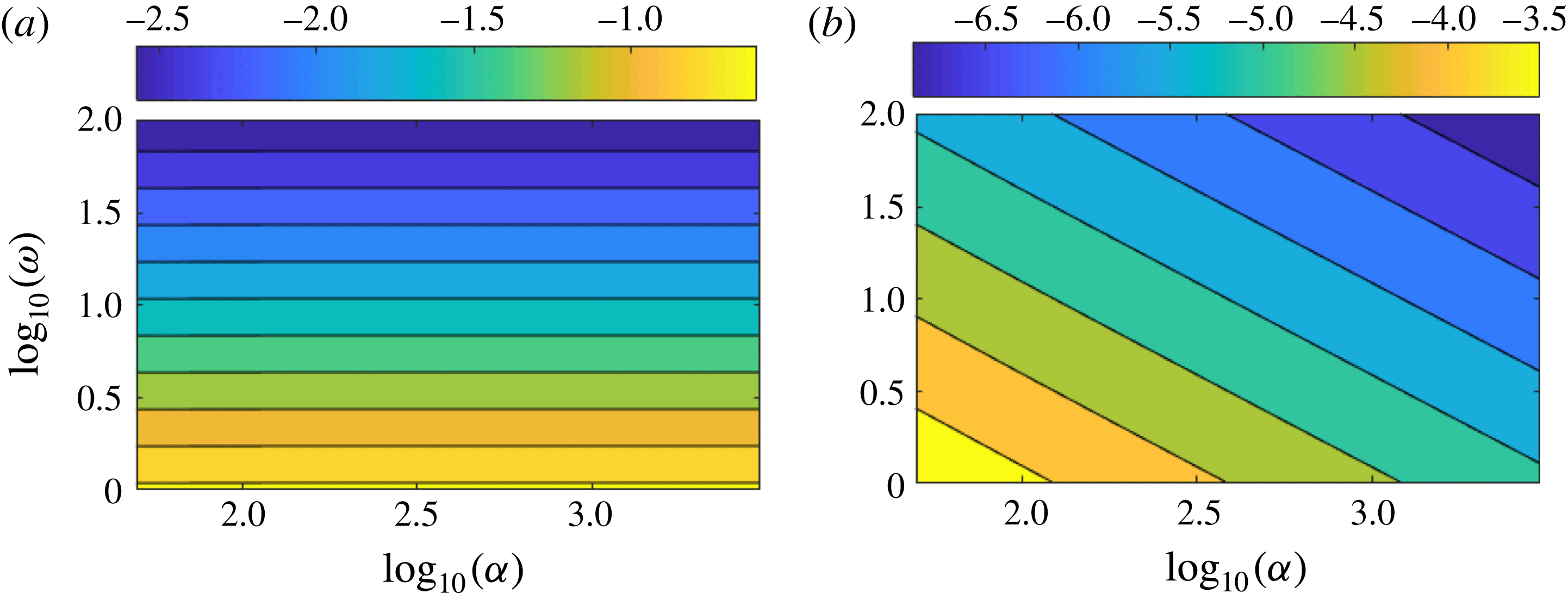
(a) Magnitude of the additional term in (3.19b
),
 $\text{log}_{10}(|Z_{1}^{\dagger }-Z_{1}|)$
. (b) Difference between the corrected boundary condition (3.19b
) and its thin boundary-layer approximation (3.27b
),
 $\text{log}_{10}(|Z_{1}^{\dagger }-Z_{1}^{\ddagger }|)$
. Both are calculated at the outer wall for
 $U_{\unicode[STIX]{x1D703}}^{nbl}=0.5$
.

The magnitude of the new term in equation (3.19b
) is presented in figure 1(a) in the
 $(\unicode[STIX]{x1D6FC},\unicode[STIX]{x1D714})$
-plane, where
 $\unicode[STIX]{x1D6FC}$
from (4.3) sets the boundary-layer thickness and
 $\unicode[STIX]{x1D714}$
is the frequency, for a typical case of
 $U_{\unicode[STIX]{x1D703}}^{nbl}=0.5$
. As expected, this term decreases with the frequency because of the
 $1/\unicode[STIX]{x1D714}$
term. However, it appears to be largely independent of the
 $\unicode[STIX]{x1D6FC}$
parameter. The additional term due to the correction is very weak almost everywhere in the
 $(\unicode[STIX]{x1D6FC},\unicode[STIX]{x1D714})$
-plane and may become significant only below
 $\unicode[STIX]{x1D714}=3$
(with
 $\text{log}_{10}(3)\approx 0.48$
), which is lower than the typical frequency range of turbofan applications. For this angular frequency
 $|Z_{1}^{\dagger }-Z_{1}|\approx 0.1$
, which must be compared with the amplitude of a typical liner impedance (
 $|Z_{1}|\approx 1$
). Close to the liner resonance defined by
 $\operatorname{Im}(Z_{1})=0$
, this additional term could become significant however.
In order to validate the thin boundary-layer approximated form of the corrected Myers boundary condition introduced in § 3.6,
 $Z_{1}^{\dagger }$
and
 $Z_{1}^{\ddagger }$
defined in (3.19b
) and (3.27b
) respectively are also compared in the
 $(\unicode[STIX]{x1D6FC},\unicode[STIX]{x1D714})$
-plane. The results are presented in figure 1(b), again for
 $U_{\unicode[STIX]{x1D703}}^{nbl}=0.5$
. As expected, the approximate solution
 $Z_{1}^{\ddagger }$
gets closer to the reference
 $Z_{1}^{\dagger }$
when the boundary-layer thickness tends to zero (e.g.
 $\unicode[STIX]{x1D6FC}\rightarrow \infty$
) and when the frequency increases. The difference between the two terms is at least 3 orders of magnitudes lower than the magnitude of the additional term for all the considered values of
 $(\unicode[STIX]{x1D6FC},\unicode[STIX]{x1D714})$
. Because of this, the simpler approximated form of the boundary condition ((3.26b
) and (3.19b
)) will be used for the numerical results that follow. This notably allows application of the boundary condition without knowing the details of the flow parameters inside the boundary layer. In both figures 1(a) and 1(b),
 $Z_{1}$
need not be specified even though it appears in the legend. Indeed, a glance at (3.19b
) and (3.27b
) will show that
 $\left|Z_{1}^{\dagger }-Z_{1}\right|$
and
 $\left|Z_{1}^{\dagger }-Z_{1}^{\ddagger }\right|$
do not depend on
 $Z_{1}$
. Besides, it is worth noting that these terms scale with
 $M_{\unicode[STIX]{x1D703},1}^{2}$
.
5.2 Validation of the corrected Myers boundary condition
First, it is proposed to assess the corrected boundary condition for a simple case. The canonical case chosen for the study is the constant swirl and constant axial flow such that
 $M_{x}=M_{\unicode[STIX]{x1D703}}=0.5$
. The duct section is characterised by the dimensionless inner radius
 $h=0.5$
. The dimensionless frequency is
 $\unicode[STIX]{x1D714}=4$
and the azimuthal mode order
 $m=-1$
is considered. The surface impedance at the inner and outer walls are defined by
 $Z_{1}=Z_{h}=1-\text{i}$
. For this case, the approximated boundary condition gives
 $Z_{h}^{\ddagger }=1-0.887\text{i}$
and
 $Z_{1}^{\ddagger }=1-1.067\text{i}$
.
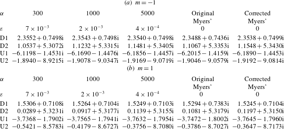
Effect of the boundary condition on the position of the most cut-on eigenmodes for the canonical case
 $M_{x}=M_{\unicode[STIX]{x1D703}}=0.5$
,
 $h=0.5$
,
 $\unicode[STIX]{x1D714}=4$
,
 $Z_{h}=Z_{1}=1-\text{i}$
, with
 $|m|=1$
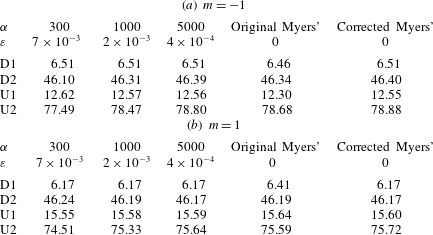
. U1: first upstream mode, U2: second upstream mode, D1: first downstream mode, D2: second downstream mode.

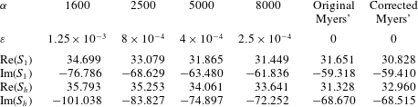
Eigenmodes obtained with the original Myers and the corrected Myers boundary conditions are compared with the ones obtained with a realistic boundary layer, for several boundary-layer thicknesses. As the boundary-layer thickness tends to zero, the eigenmodes become harder to calculate numerically when simulating the boundary layer. In table 1, the two most ‘cut-on’ upstream and downstream eigenmodes are considered.
The additional centrifugal term in the corrected Myers boundary condition has an effect on the eigenmodes, since they differ from the eigenmodes of the classical Myers boundary condition at the second decimal in this case. Furthermore, when the boundary-layer thickness tends to zero, the eigenmodes indeed converge towards the eigenmodes from the corrected Myers boundary condition.
For a given eigenmode, the corresponding attenuation rate in dB is given by
 $\pm 20\operatorname{Im}(k)/\text{log}(10)$
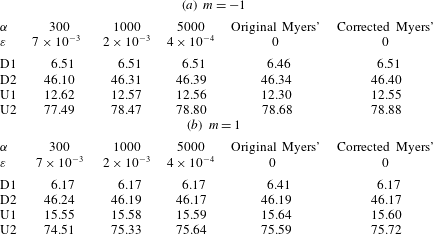
, the sign depending on the direction of propagation. The attenuation rates related to the eigenmodes of table 1 are presented in table 2. As for the eigenmodes, the attenuation rates converge towards the corrected Myers boundary condition when the boundary-layer thickness tends to zero.
These observations suggest that (3.26) and (3.27) are the correct limits for a vanishing boundary layer.
Attenuation rates in dB per radius for the different boundary conditions with the parameters as in table 1.
5.3 Centrifugal effect on the eigenmodes at lower frequency
Because of the
 $\unicode[STIX]{x1D714}^{-1}$
factor contained in the centrifugal term in (3.26) and (3.27), larger differences are expected between the original Myers boundary condition and the corrected Myers boundary condition in the low frequency range. To illustrate this, the above test case is considered again, but with a frequency ten times lower (
 $\unicode[STIX]{x1D714}=0.4$
), all the other parameters being unchanged. The eigenmodes obtained with both boundary conditions are plotted in figure 2. They are compared to the reference eigenmodes, which are also obtained by solving numerically the set of (2.9) according to the method described at the beginning of § 4. These reference eigenmodes are computed for a realistic flow profile defined by
 $U_{x}(r)=U_{\unicode[STIX]{x1D703}}(r)=0.5L_{2500}(r)$
, where
 $L_{2500}$
represents a thin boundary layer (displacement thickness
 $\unicode[STIX]{x1D700}=4\times 10^{-4}$
), together with the boundary conditions
 $Z_{eff}(h)=Z_{h}$
and
 $Z_{eff}(1)=Z_{1}$
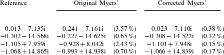
since the mean flow cancels at both walls. The values of some of the eigenmodes are given in table 3 for the three boundary conditions.
Eigenmode positions in the complex
 $k$
-plane at low frequency (
 $\unicode[STIX]{x1D714}=0.4$
). The case is defined by
 $M_{x}=M_{\unicode[STIX]{x1D703}}=0.5$
,
 $h=0.5$
,
 $m=-1$
,
 $Z_{h}=Z_{1}=1-\text{i}$
. A total of 300 points were used for the radial discretisation.

Effect of the boundary condition on the position of some eigenmodes for the low frequency case (
 $\unicode[STIX]{x1D714}=0.4$
).
 $M_{x}=M_{\unicode[STIX]{x1D703}}=0.5$
,
 $h=0.5$
,
 $m=-1$
,
 $Z_{h}=Z_{1}=1-\text{i}$
. The relative errors to the reference eigenvalues are shown in brackets.

As expected, the centrifugal effects in the boundary condition are much stronger than for the previous frequency of observation. Indeed, for this specific case,
 $Z_{h}^{\ddagger }=1+0.13\text{i}$
and
 $Z_{1}^{\ddagger }=1-1.67\text{i}$
. The original Myers boundary condition inaccurately predicts the eigenmodes while the new corrected boundary condition gives eigenmodes much closer to the reference.
5.4 Illustration of the correct behaviour for vanishing boundary layers
In this section, the exact value of
 $Z_{eff}^{1}=\hat{p}_{\infty }^{1}/\hat{u} _{\infty }^{1}$
, which would be obtained if there was no boundary layer, is compared with the effective impedance arising from the different boundary conditions. To isolate the boundary condition being investigated at
 $r=1$
, a slipping mean flow with no boundary layer is assumed at
 $r=h$
and two artificial boundary conditions are introduced there, given by
 $\hat{p}(h)=1-\text{i}$
and
 $\hat{u} (h)=-1$
. For any given values of
 $\unicode[STIX]{x1D714}$
,
 $m$
and
 $k$
, the governing (2.11) and (2.12) may be integrated to give
 $\hat{p}(r)$
and
 $\hat{u} (r)$
. Hence, the exact value of
 $\hat{p}_{\infty }^{1}$
and
 $\hat{v}_{\infty }^{1}$
(and hence
 $Z_{eff}^{1}=\hat{p}_{\infty }^{1}/\hat{u} _{\infty }^{1}$
) can be computed by taking no boundary layer near
 $r=1$
. By introducing an exponential boundary layer similar to
 $L_{\unicode[STIX]{x1D6FC}}$
at
 $r=1$
, the exact value of
 $Z_{BL}^{1}=\hat{p}_{\unicode[STIX]{x1D6FC}}(1)/\hat{u} _{\unicode[STIX]{x1D6FC}}(1)$
can be computed in the same way.
Thus, the accuracy of the boundary conditions can be assessed by comparing the exact value
 $Z_{eff}^{1}=\hat{p}_{\infty }^{1}/\hat{u} _{\infty }^{1}$
with the ones which would be obtained by inserting
 $Z_{BL}^{1}$
in the boundary conditions. The new boundary condition, the approximated boundary condition and the classical Myers boundary condition are written in terms of an effective impedance. They read
 $$\begin{eqnarray}\displaystyle & \displaystyle Z_{eff}^{\dagger ,1}=-{\displaystyle \frac{\unicode[STIX]{x1D714}}{\unicode[STIX]{x1D6EC}_{\infty }^{1}}}\left(Z_{BL}^{1}+{\displaystyle \frac{\text{i}}{\unicode[STIX]{x1D714}}}\int _{r_{m}}^{1}\unicode[STIX]{x1D70C}_{0}{\displaystyle \frac{\text{d}}{\text{d}r}}\left(U_{\unicode[STIX]{x1D703}}^{2}\right)\text{d}r\right), & \displaystyle\end{eqnarray}$$
 $$\begin{eqnarray}\displaystyle & \displaystyle Z_{eff}^{\ddagger ,1}=-{\displaystyle \frac{\unicode[STIX]{x1D714}}{\unicode[STIX]{x1D6EC}_{\infty }^{1}}}\left(Z_{BL}^{1}-{\displaystyle \frac{\text{i}}{\unicode[STIX]{x1D714}}}\unicode[STIX]{x1D70C}_{0}^{nbl}(1)M_{\unicode[STIX]{x1D703},1}^{2}\right), & \displaystyle\end{eqnarray}$$
 $$\begin{eqnarray}\displaystyle & \displaystyle Z_{eff}^{M,1}=-{\displaystyle \frac{\unicode[STIX]{x1D714}Z_{BL}^{1}}{\unicode[STIX]{x1D6EC}_{\infty }^{1}}}, & \displaystyle\end{eqnarray}$$
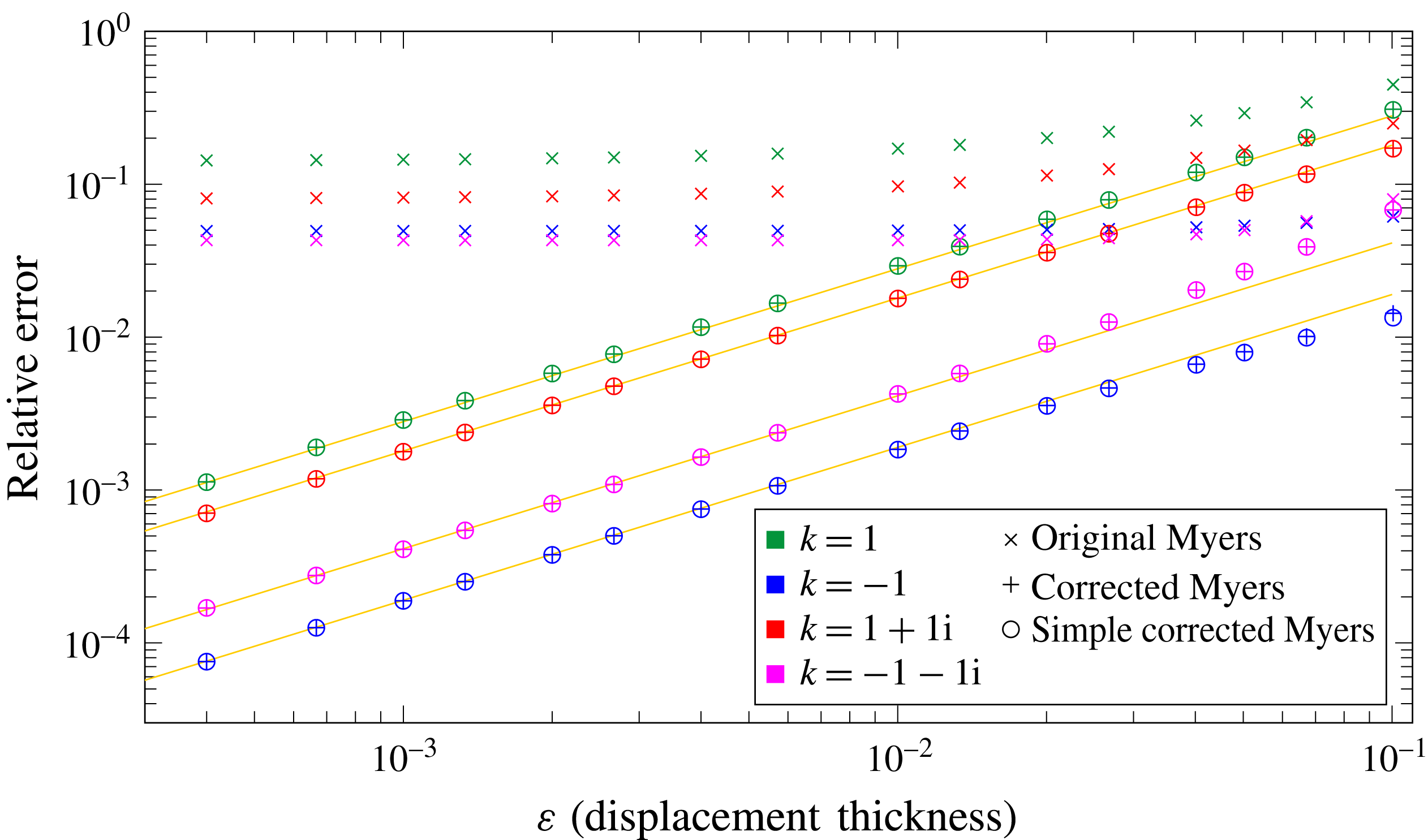
respectively. For these three boundary conditions, the equivalent impedance is compared with
 $Z_{eff}^{1}$
. In figure 3, the evolution of the errors
 $|Z_{eff}^{\dagger ,1}/Z_{eff}^{1}-1|$
,
 $|Z_{eff}^{\ddagger ,1}/Z_{eff}^{1}-1|$
and
 $|Z_{eff}^{M,1}/Z_{eff}^{1}-1|$
as a function of the boundary-layer thickness are shown for four values of
 $k$
:
 $1$
,
 $-1$
,
 $1+\text{i}$
and
 $-1-\text{i}$
. The parameters used for the study are
 $h=0.5$
,
 $\unicode[STIX]{x1D714}=5$
,
 $m=1$
and
 $M_{x}=M_{\unicode[STIX]{x1D703}}=0.5$
.
Plot of the relative error
 $|Z_{eff}^{\dagger ,1}/Z_{eff}^{1}-1|$
(plusses),
 $|Z_{eff}^{\ddagger ,1}/Z_{eff}^{1}-1|$
(circles) and
 $|Z_{eff}^{M,1}/Z_{eff}^{1}-1|$
(crosses) at the outer wall. The other parameters are
 $h=0.5$
,
 $\unicode[STIX]{x1D714}=5$
,
 $m=1$
and
 $M_{x}=M_{\unicode[STIX]{x1D703}}=0.5$
.

Since the corrected Myers boundary condition has been developed to leading order with error
 $O(\unicode[STIX]{x1D6FF})$
, it is expected that the error decreases linearly with the boundary-layer thickness. The linear relationship between the error and the boundary-layer thickness is drawn in yellow. The corrected Myers boundary condition as well as its simple approximation match very well the expected behaviour while the classical Myers condition is clearly wrong.
Applying the same procedure at the inner wall leads to the same conclusions. Comparisons have not been shown here for the sake of conciseness.
5.5 A realistic turbofan engine configuration: the SDT test case
Finally, the corrected Myers boundary condition is tested on a realistic fan configuration. The mean flow has been extracted from the core flow of a Reynolds-averaged Navier–Stokes (RANS) simulation performed on the NASA SDT test case (see Hughes et al.
Reference Hughes, Jeracki, Woodward and Miller2002; Woodward et al.
Reference Woodward, Hughes, Jeracki and Miller2002) so that the flow is representative of a bypass interstage with no boundary layer. After interpolating the mean flow on a set of rational functions, a boundary layer can be added by multiplying the mean flow by the exponential envelope defined in (4.3). The value of
 $\unicode[STIX]{x1D6FC}=200$
was chosen since it corresponds to a displacement thickness of
 $\unicode[STIX]{x1D700}=0.01$
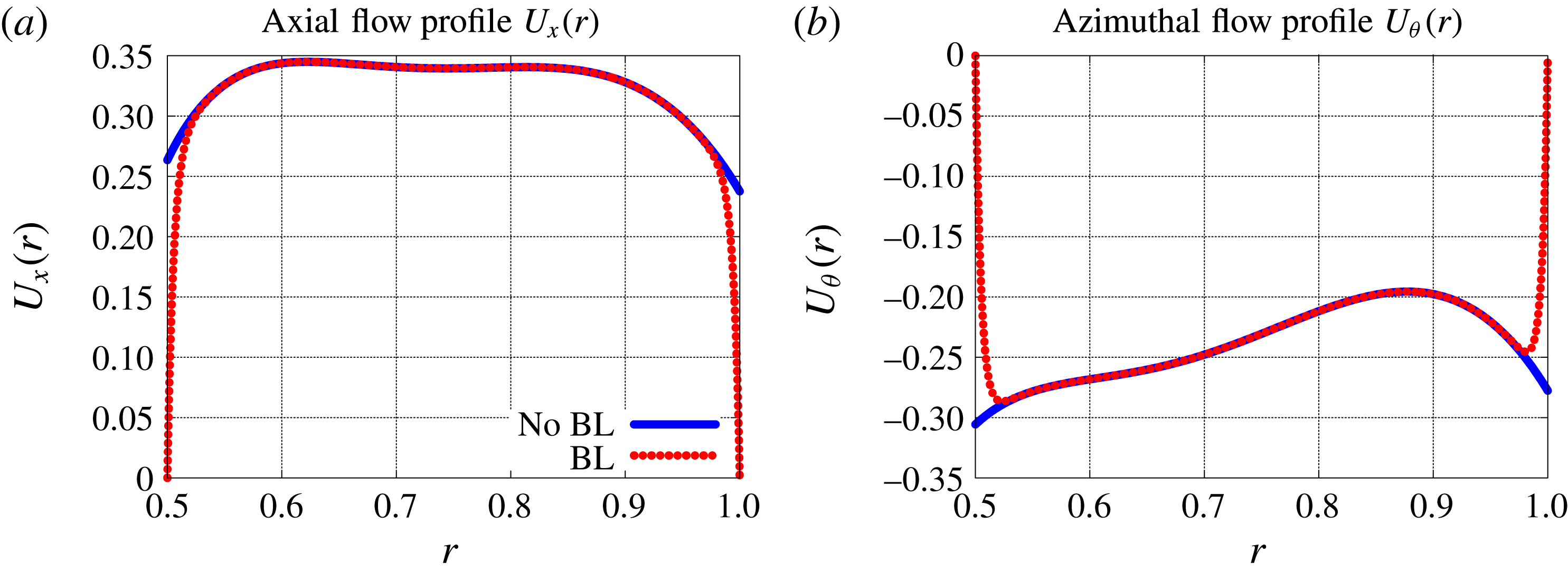
, which is representative of a boundary-layer thickness in the interstage. The mean flow profiles with and without the boundary layer are shown in figures 4(a) and 4(b).
Interpolated profiles from the SDT test case, with or without a boundary layer.

The hub-to-tip ratio of the SDT test case is
 $h=0.5$
. The frequency of the study is chosen so that it fits with the maximum of the rotor–stator interaction broadband noise spectra at approach condition. The value
 $f_{\text{max}}^{\star }=3000~\text{Hz}$
has been taken from Masson et al. (Reference Masson, Posson, Sanjose, Moreau and Roger2016), which corresponds to
 $\unicode[STIX]{x1D714}=15$
. Even though there is no acoustic treatment in the NASA SDT, the walls are assumed to be lined with typical acoustic treatments. The impedance is set to
 $Z_{h}=Z_{1}=2.55+1.5\text{i}$
. The imaginary part is above zero which corresponds to a resonance at a higher frequency. The effect of the boundary condition on the eigenmodes and the eigenfunctions will be assessed for
 $m=1$
and
 $m=15$
. Since the azimuthal flow is negative, these values correspond to contra-rotating modes according to the conventions of the paper.
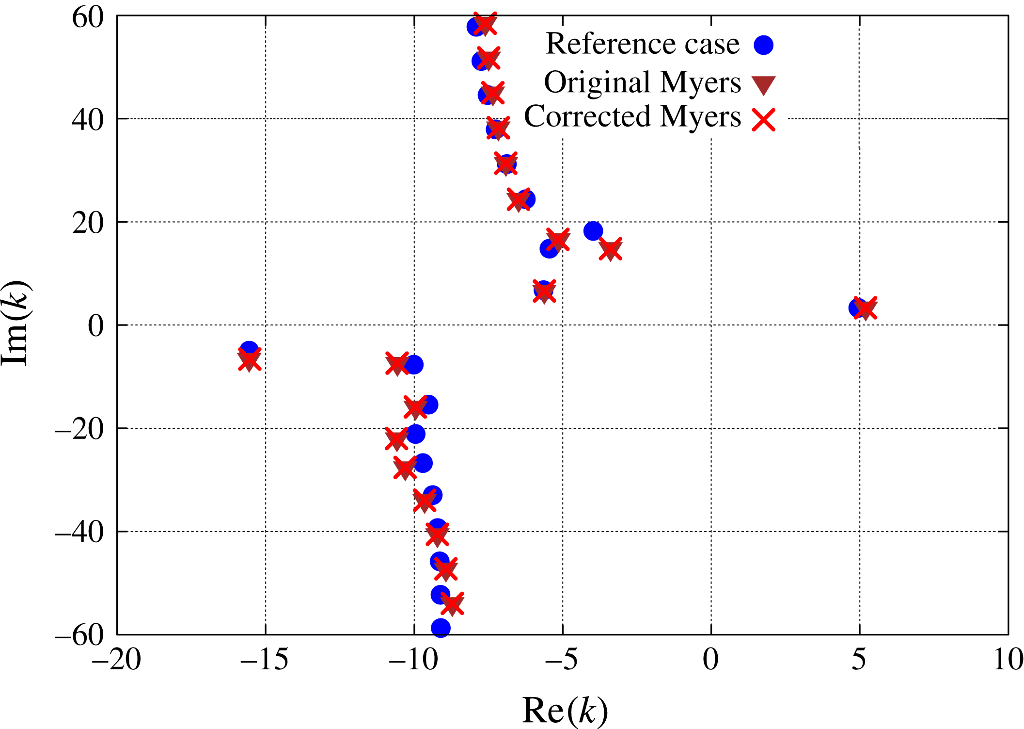
5.5.1 Position of the eigenmodes
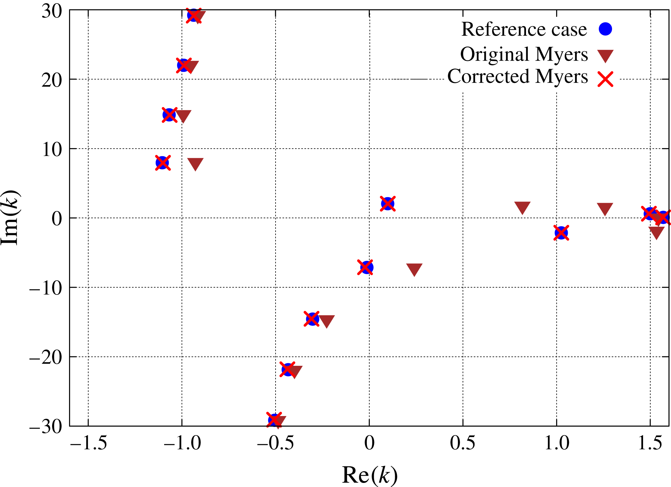
The azimuthal mode
 $m=1$
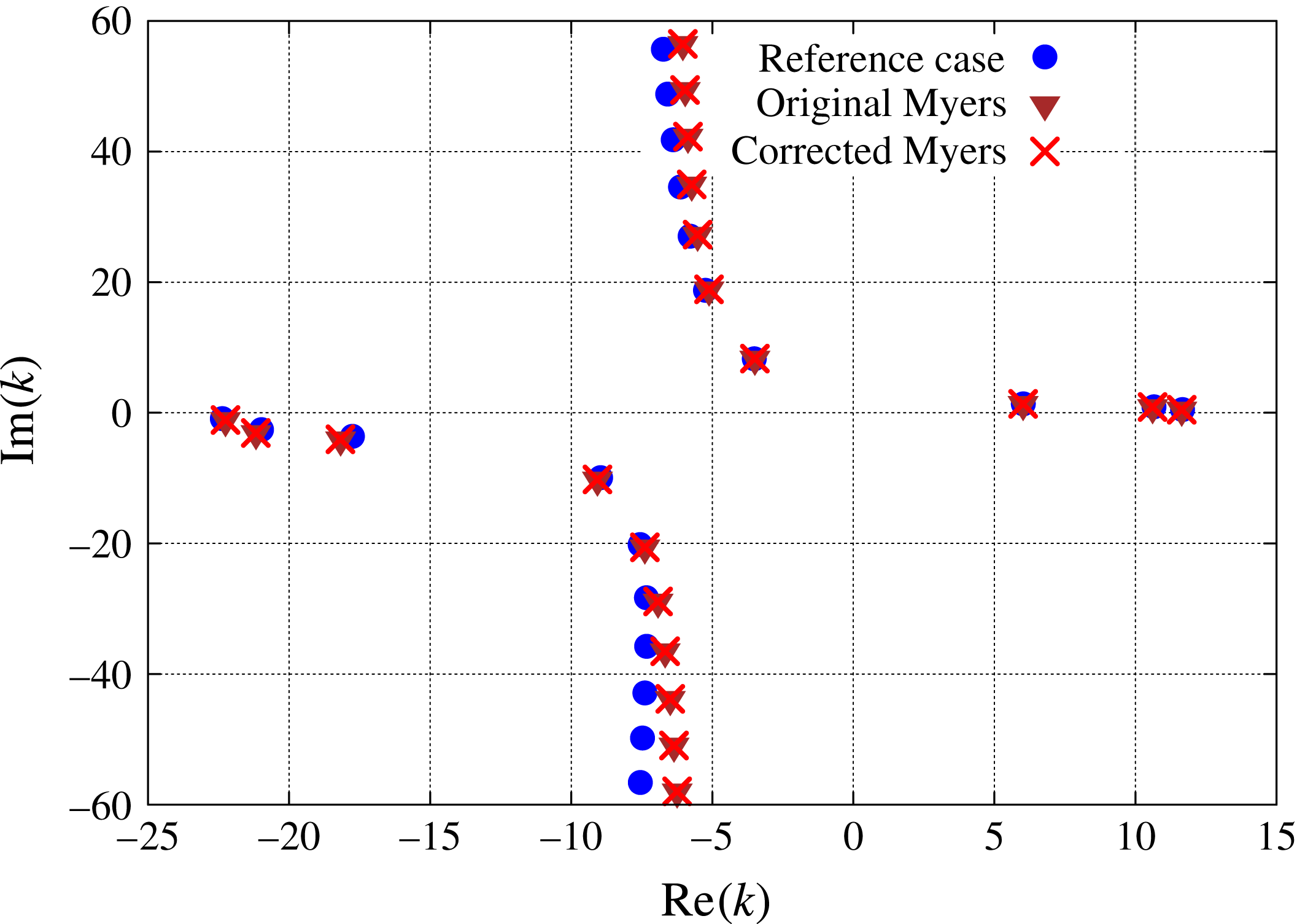
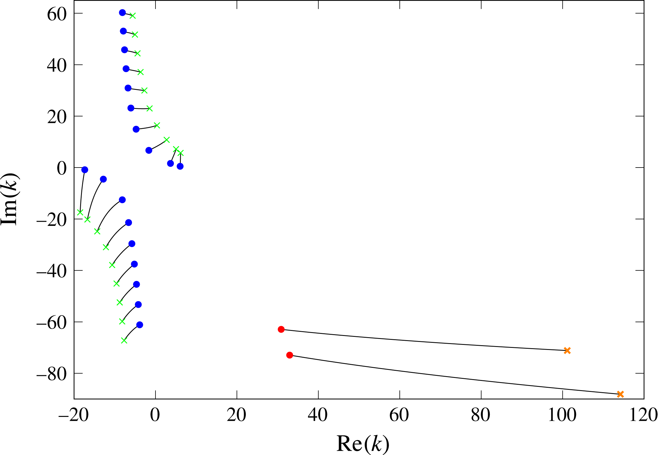
is considered first. The eigenmodes of (4.1) are plotted in figure 5 for the three boundary conditions. The original Myers boundary condition ((3.2), violet triangles) and the corrected Myers boundary condition ((3.27), red crosses) are compared with the reference ((3.1), blue circles) which is obtained by considering the flow with a boundary layer. For these three cases, the same boundary condition is applied both at the inner and outer walls. Since the frequency is quite high, results obtained from the original Myers boundary condition and from the corrected Myers boundary condition are very similar, the eigenmodes being almost indistinguishable. The ‘most’ cut-on modes, which are the most relevant when studying in-duct transmission, are pretty well predicted, especially in the downstream direction, while the accuracy decreases as the modes move away from the real axis.
Eigenmode positions in the complex
 $k$
-plane for a realistic test case based on the SDT mean flow. The case is defined by
 $\unicode[STIX]{x1D714}=15$
,
 $h=0.5$
,
 $m=1$
,
 $Z_{h}=Z_{1}=2.55+1.5\text{i}$
.

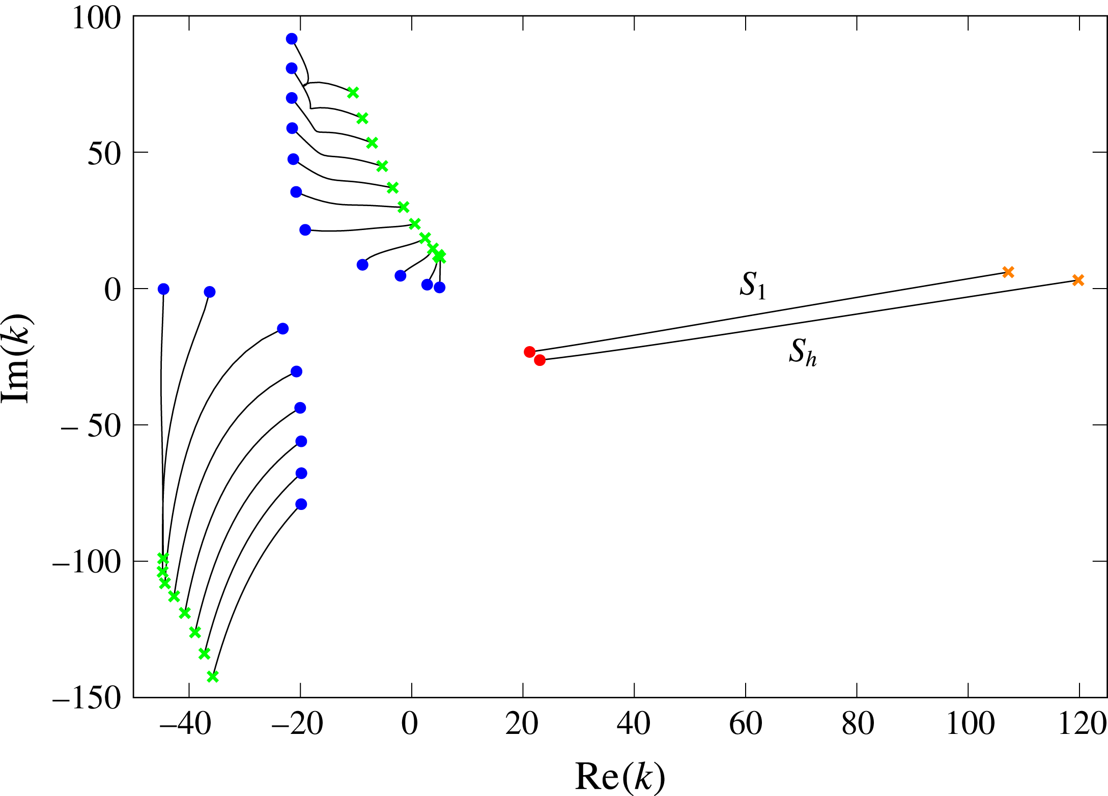
Eigenmode positions in the complex
 $k$
-plane for a realistic test case based on the SDT mean flow. The case is defined by
 $\unicode[STIX]{x1D714}=15$
,
 $h=0.5$
,
 $m=15$
,
 $Z_{h}=Z_{1}=2.55+1.5\text{i}$
.

The same methodology is then applied to the azimuthal mode order
 $m=15$
. The results are presented in figure 6. Once again, the original Myers boundary condition gives very similar results as the corrected one. However, significant error is observed with respect to the reference case, even for the eigenmodes located close to the real axis. This is expected to alter the prediction when acoustic transmission is considered. To improve the accuracy of the corrected Myers boundary condition with swirl, it is possible to extend the method presented in § 3 to the first order in
 $\unicode[STIX]{x1D6FF}$
, as done by Brambley (Reference Brambley2011) in the case of no swirl.
6 Surface waves in an annular duct with swirl
The modes corresponding to surface waves in swirling flows are now considered. These are a different class of modes from the acoustic modes that have so far been considered. Surface waves only occur in a lined duct and their mode shape is localised about the duct boundary. These surface-wave modes still satisfy (4.1), but they are often difficult to resolve numerically, meaning that a good initial guess is often needed, which comes from an analytical dispersion relation for the surface-wave modes.
Surface waves were first considered in detail by Rienstra (Reference Rienstra2003) for uniform axial flow in a lined duct with Myers’ boundary condition in the high frequency range, and small azimuthal number limit. This was then extended by Brambley & Peake (Reference Brambley and Peake2006) to arbitrary azimuthal wavenumber, but still for a uniform axial flow in a hollow duct. Our aim in this section is to extend the dispersion relation and results from Brambley & Peake (Reference Brambley and Peake2006) to swirling flow in an annular duct.
6.1 The surface-wave dispersion relation with swirl
The surface-wave dispersion relation is considered first at the outer wall. The surface waves located near the outer wall are characterised by an exponential decay away from the outer wall, so that the acoustic pressure and normal velocity
 $\hat{p}$
and
 $\hat{u}$
are of the form
 $$\begin{eqnarray}\displaystyle & \displaystyle \hat{p}(r)=\unicode[STIX]{x1D713}_{\hat{p}}(r)\text{e}^{-\unicode[STIX]{x1D707}_{1}(1-r)},\quad \hat{u} (r)=\unicode[STIX]{x1D713}_{\hat{u} }(r)\text{e}^{-\unicode[STIX]{x1D707}_{1}(1-r)} & \displaystyle\end{eqnarray}$$
respectively, where
 $\unicode[STIX]{x1D707}_{1}$
is the radial wavenumber near the outer wall and
 $\text{d}\unicode[STIX]{x1D713}_{\unicode[STIX]{x1D711}}/\text{d}r=O(1)$
for
 $\unicode[STIX]{x1D711}=\hat{p},\hat{u}$
. For surface waves to decay exponentially from the wall, it is required that
 $\text{Re}(\unicode[STIX]{x1D707}_{1})>0$
and
 $|\text{Re}(\unicode[STIX]{x1D707}_{1})|\gg 1$
. Note that, for the infinitely thin boundary-layer assumption
 $\unicode[STIX]{x1D6FF}\ll 1$
to still hold for such surface waves,
 $\unicode[STIX]{x1D6FF}\ll 1/|\unicode[STIX]{x1D707}_{1}|\ll 1$
is required. From these assumptions, the derivative of
 $\hat{p}$
and
 $\hat{u}$
can be evaluated near the outer wall
 $$\begin{eqnarray}\displaystyle {\displaystyle \frac{\text{d}\hat{p}}{\text{d}r}}(1)=\unicode[STIX]{x1D707}_{1}\hat{p}(1)+O(1),\quad {\displaystyle \frac{\text{d}\hat{u} }{\text{d}r}}(1)=\unicode[STIX]{x1D707}_{1}\hat{u} (1)+O(1). & & \displaystyle\end{eqnarray}$$
The boundary conditions at the inner wall impose conditions on
 $\unicode[STIX]{x1D713}_{\hat{p}}(h)$
and
 $\unicode[STIX]{x1D713}_{\hat{u} }(h)$
, but since both
 $\hat{p}$
and
 $\hat{u}$
are exponentially small away from
 $r=1$
this inner boundary condition does not affect the dominant behaviour near
 $r=1$
. This decoupling of the boundary conditions for the surface waves was also shown by Rienstra (Reference Rienstra2003, § 9) in the case of uniform flow in an annular duct, and can be verified explicitly from the high frequency approximation as in Heaton & Peake (Reference Heaton and Peake2005), Mathews & Peake (Reference Mathews and Peake2017) for arbitrary swirling flows.
Equations (2.10) and (2.12) can be rewritten at the outer wall for the specific case of surface waves propagating in a homentropic mean flow. To leading order the pressure and normal velocity satisfy
 $$\begin{eqnarray}\displaystyle \displaystyle & & \displaystyle \left({\displaystyle \frac{\unicode[STIX]{x1D6EC}^{2}(1)}{c_{0}^{2}(1)}}-m^{2}-k^{2}\right)\hat{p}+\left[-\unicode[STIX]{x1D707}_{1}\unicode[STIX]{x1D6EC}(1)-\unicode[STIX]{x1D6EC}(1)-{\displaystyle \frac{U_{\unicode[STIX]{x1D703}}^{2}(1)}{c_{0}^{2}(1)}}\unicode[STIX]{x1D6EC}(1)\right.\nonumber\\ \displaystyle & & \displaystyle \qquad \left.+\,k{\displaystyle \frac{\text{d}U_{x}}{\text{d}r}}(1)+m\left({\displaystyle \frac{\text{d}U_{\unicode[STIX]{x1D703}}}{\text{d}r}}(1)+U_{\unicode[STIX]{x1D703}}(1)\right)\right]\text{i}\unicode[STIX]{x1D70C}_{0}(1)\hat{u} =0,\end{eqnarray}$$
 $$\begin{eqnarray}\displaystyle & & \displaystyle \displaystyle \left(\unicode[STIX]{x1D707}_{1}\unicode[STIX]{x1D6EC}(1)+2mU_{\unicode[STIX]{x1D703}}(1)-{\displaystyle \frac{U_{\unicode[STIX]{x1D703}}^{2}(1)\unicode[STIX]{x1D6EC}(1)}{c_{0}^{2}(1)}}\right)\hat{p}\nonumber\\ \displaystyle & & \displaystyle \qquad +\,\left(\unicode[STIX]{x1D6EC}^{2}(1)-2U_{\unicode[STIX]{x1D703}}(1){\displaystyle \frac{\text{d}U_{\unicode[STIX]{x1D703}}}{\text{d}r}}(1)-2U_{\unicode[STIX]{x1D703}}^{2}(1)\right)\text{i}\unicode[STIX]{x1D70C}_{0}(1)\hat{u} =0.\end{eqnarray}$$
At the outer wall, the approximate corrected Myers boundary condition reads:
 $$\begin{eqnarray}\displaystyle & \displaystyle \text{i}\unicode[STIX]{x1D714}\unicode[STIX]{x1D70C}_{0}(1)Z_{1}^{\ddagger }\hat{u} (1)=-\text{i}\unicode[STIX]{x1D70C}_{0}(1)\unicode[STIX]{x1D6EC}(1)\hat{p}(1), & \displaystyle\end{eqnarray}$$
where
 $Z_{1}^{\ddagger }$
is defined in (3.27b
). This is substituted in (6.3) and (6.4), and after eliminating
 $\hat{p}$
the coupled velocity and pressure equations read
 $$\begin{eqnarray}\displaystyle & & \displaystyle \displaystyle {\displaystyle \frac{\unicode[STIX]{x1D6EC}^{2}(1)}{c_{0}^{2}(1)}}-m^{2}-k^{2}+\left[-\unicode[STIX]{x1D707}_{1}\unicode[STIX]{x1D6EC}(1)-\unicode[STIX]{x1D6EC}(1)-{\displaystyle \frac{U_{\unicode[STIX]{x1D703}}^{2}(1)}{c_{0}^{2}(1)}}\unicode[STIX]{x1D6EC}(1)\right.\nonumber\\ \displaystyle & & \displaystyle \quad \left.+\,k{\displaystyle \frac{\text{d}U_{x}}{\text{d}r}}(1)+m\left({\displaystyle \frac{\text{d}U_{\unicode[STIX]{x1D703}}}{\text{d}r}}(1)+U_{\unicode[STIX]{x1D703}}(1)\right)\right]\left(-\text{i}{\displaystyle \frac{\unicode[STIX]{x1D70C}_{0}(1)\unicode[STIX]{x1D6EC}(1)}{\unicode[STIX]{x1D714}Z_{1}^{\ddagger }}}\right)=0,\end{eqnarray}$$
and
 $$\begin{eqnarray}\displaystyle & & \displaystyle \unicode[STIX]{x1D707}_{1}\unicode[STIX]{x1D6EC}(1)+2mU_{\unicode[STIX]{x1D703}}(1)-{\displaystyle \frac{U_{\unicode[STIX]{x1D703}}^{2}(1)\unicode[STIX]{x1D6EC}(1)}{c_{0}^{2}(1)}}\nonumber\\ \displaystyle & & \displaystyle \quad +\,\left(\unicode[STIX]{x1D6EC}^{2}(1)-2U_{\unicode[STIX]{x1D703}}(1){\displaystyle \frac{\text{d}U_{\unicode[STIX]{x1D703}}}{\text{d}r}}(1)-2U_{\unicode[STIX]{x1D703}}^{2}(1)\right)\left(-\text{i}{\displaystyle \frac{\unicode[STIX]{x1D70C}_{0}(1)\unicode[STIX]{x1D6EC}(1)}{\unicode[STIX]{x1D714}Z_{1}^{\ddagger }}}\right)=0.\end{eqnarray}$$
Finally, the dispersion relation for the surface waves at the outer wall is obtained by eliminating
 $\unicode[STIX]{x1D707}_{1}$
in (6.6) and (6.7). It reads:
 $$\begin{eqnarray}\displaystyle & & \displaystyle \displaystyle \text{i}{\displaystyle \frac{\unicode[STIX]{x1D714}Z_{1}^{\ddagger }}{\unicode[STIX]{x1D70C}_{0}}}\left[\text{i}{\displaystyle \frac{\unicode[STIX]{x1D714}Z_{1}^{\ddagger }}{\unicode[STIX]{x1D70C}_{0}}}\left({\displaystyle \frac{\unicode[STIX]{x1D6EC}^{2}}{c_{0}^{2}}}-m^{2}-k^{2}\right)-\unicode[STIX]{x1D6EC}^{2}\left(1+{\displaystyle \frac{2U_{\unicode[STIX]{x1D703}}^{2}}{c_{0}^{2}}}\right)\right.\nonumber\\ \displaystyle & & \displaystyle \quad \left.+\,\unicode[STIX]{x1D6EC}\left(k{\displaystyle \frac{\text{d}U_{x}}{\text{d}r}}+3mU_{\unicode[STIX]{x1D703}}+m{\displaystyle \frac{\text{d}U_{\unicode[STIX]{x1D703}}}{\text{d}r}}\right)\vphantom{{\displaystyle \frac{\unicode[STIX]{x1D714}Z_{1}^{\ddagger }}{\unicode[STIX]{x1D70C}_{0}}}}\right]+\unicode[STIX]{x1D6EC}^{2}\left(\unicode[STIX]{x1D6EC}^{2}-2U_{\unicode[STIX]{x1D703}}{\displaystyle \frac{\text{d}U_{\unicode[STIX]{x1D703}}}{\text{d}r}}-2U_{\unicode[STIX]{x1D703}}^{2}\right)=0,\end{eqnarray}$$
where all the quantities are evaluated at
 $r=1$
.
Similarly, the dispersion relation for surface waves located near the inner wall can be derived. The acoustic variables are now proportional to
 $\exp \{-\unicode[STIX]{x1D707}_{h}(r-h)\}$
, where
 $\text{Re}(\unicode[STIX]{x1D707}_{h})>0$
and
 $|\text{Re}(\unicode[STIX]{x1D707}_{h})|\gg 1$
. Following the same approach as for the outer wall yields:
 $$\begin{eqnarray}\displaystyle & & \displaystyle \displaystyle -\text{i}{\displaystyle \frac{\unicode[STIX]{x1D714}Z_{h}^{\ddagger }}{\unicode[STIX]{x1D70C}_{0}}}\left[-\text{i}{\displaystyle \frac{\unicode[STIX]{x1D714}Z_{h}^{\ddagger }}{\unicode[STIX]{x1D70C}_{0}}}\left({\displaystyle \frac{\unicode[STIX]{x1D6EC}^{2}}{c_{0}^{2}}}-{\displaystyle \frac{m^{2}}{h^{2}}}-k^{2}\right)-\unicode[STIX]{x1D6EC}^{2}\left({\displaystyle \frac{1}{h}}+{\displaystyle \frac{2U_{\unicode[STIX]{x1D703}}^{2}}{hc_{0}^{2}}}\right)\right.\nonumber\\ \displaystyle & & \displaystyle \quad \left.+\,\unicode[STIX]{x1D6EC}\left(k{\displaystyle \frac{\text{d}U_{x}}{\text{d}r}}+{\displaystyle \frac{3mU_{\unicode[STIX]{x1D703}}}{h^{2}}}+{\displaystyle \frac{m}{h}}{\displaystyle \frac{\text{d}U_{\unicode[STIX]{x1D703}}}{\text{d}r}}\right)\vphantom{{\displaystyle \frac{\unicode[STIX]{x1D714}Z_{1}^{\ddagger }}{\unicode[STIX]{x1D70C}_{0}}}}\right]+\unicode[STIX]{x1D6EC}^{2}\left(\unicode[STIX]{x1D6EC}^{2}-{\displaystyle \frac{2U_{\unicode[STIX]{x1D703}}}{h}}{\displaystyle \frac{\text{d}U_{\unicode[STIX]{x1D703}}}{\text{d}r}}-{\displaystyle \frac{2U_{\unicode[STIX]{x1D703}}^{2}}{h^{2}}}\right)=0,\end{eqnarray}$$
where all the quantities are evaluated at
 $r=h$
. Equations (6.8) and (6.9) are polynomials in
 $k$
of degree four. Therefore there are at most four surface-wave modes at each wall, although some of the solutions may not satisfy
 $\text{Re}(\unicode[STIX]{x1D707}_{r_{0}})>0,r_{0}=\{h,1\}$
where
 $\unicode[STIX]{x1D707}_{1}$
is given by (6.7) for instance.
6.2 No-swirl case
If the swirl is set to zero, equations (6.8) and (6.9) reduce to
 $$\begin{eqnarray}\displaystyle & \displaystyle \pm \text{i}{\displaystyle \frac{\unicode[STIX]{x1D714}Z_{r_{0}}}{\unicode[STIX]{x1D70C}_{0}}}\left[\pm \text{i}{\displaystyle \frac{\unicode[STIX]{x1D714}Z_{r_{0}}}{\unicode[STIX]{x1D70C}_{0}}}\left({\displaystyle \frac{\unicode[STIX]{x1D6EC}^{2}}{c_{0}^{2}}}-{\displaystyle \frac{m^{2}}{r_{0}^{2}}}-k^{2}\right)-{\displaystyle \frac{\unicode[STIX]{x1D6EC}^{2}}{r_{0}}}+\unicode[STIX]{x1D6EC}k{\displaystyle \frac{\text{d}U_{x}}{\text{d}r}}\right]+\unicode[STIX]{x1D6EC}^{4}=0, & \displaystyle\end{eqnarray}$$
(where
 $\pm =+$
at the outer wall and
 $\pm =-$
at the inner wall), which can also be written in the form
 $$\begin{eqnarray}\displaystyle \unicode[STIX]{x1D707}_{r_{0}}=\text{i}{\displaystyle \frac{\unicode[STIX]{x1D70C}_{0}\unicode[STIX]{x1D6EC}^{2}}{\unicode[STIX]{x1D714}Z_{1}}},\quad \unicode[STIX]{x1D707}_{r_{0}}^{2}={\displaystyle \frac{m^{2}}{r_{0}^{2}}}+k^{2}-{\displaystyle \frac{\unicode[STIX]{x1D6EC}^{2}}{c_{0}^{2}}}\pm \unicode[STIX]{x1D707}_{r_{0}}\left({\displaystyle \frac{k}{\unicode[STIX]{x1D6EC}}}{\displaystyle \frac{\text{d}U_{x}}{\text{d}r}}-{\displaystyle \frac{1}{r_{0}}}\right). & & \displaystyle\end{eqnarray}$$
Equation (6.11) is equivalent at leading order in
 $1/\unicode[STIX]{x1D707}_{r_{0}}$
to the surface-wave dispersion relation of Brambley & Peake (Reference Brambley and Peake2006), as used by Brambley (Reference Brambley2013). Since both equation (6.11) and the surface-wave dispersion relation of Brambley & Peake (Reference Brambley and Peake2006) were derived only to leading order in
 $1/\unicode[STIX]{x1D707}_{r_{0}}$
by different methods, it is unsurprising that they differ at high orders of
 $1/\unicode[STIX]{x1D707}_{r_{0}}$
, and such differences are not significant. The difference between the two is due to the presence of the
 $1/r_{0}$
and
 $kU_{x}^{\prime }/\unicode[STIX]{x1D6EC}$
terms. These terms physically correspond to geometric effects of the curved cylindrical surface and mean flow shear effects at the wall respectively.
6.3 Results
Some results for the surface waves are now considered. The surface-wave modes predicted from the analytical dispersion relation are first compared with the exact numerical eigenmodes. The differences in surface-wave modes for the original Myers boundary condition and the corrected Myers boundary condition are then examined. Finally, the number of surface-wave modes predicted by the dispersion relations are studied for different impedances.
6.3.1 Comparison between asymptotic and numerical surface waves
The asymptotic surface-wave modes predicted from the dispersion relations in (6.8) and (6.9) are first compared with the exact numerical modes for an infinitely thin boundary layer. The following parameters are used:
 $M_{x}=0.5$
,
 $M_{\unicode[STIX]{x1D703}}=0.5$
,
 $h=0.5$
,
 $m=1$
and
 $\unicode[STIX]{x1D714}=10$
. An impedance specified by a mass–spring–damper,
 $Z(\unicode[STIX]{x1D714})=R_{Z}-\text{i}M_{Z}\unicode[STIX]{x1D714}+\text{i}K_{Z}/\unicode[STIX]{x1D714}$
is also taken, where
 $R_{Z}$
is the impedance damping,
 $M_{Z}$
the impedance mass and
 $K_{Z}$
the impedance spring. The parameters
 $R_{Z}=1.6$
,
 $K_{Z}=6$
and
 $M_{Z}=0.08$
are chosen from Table 1 in Brambley & Gabard (Reference Brambley and Gabard2016), giving
 $Z(10)=1.6-0.2\text{i}$
. Note that because of the different time convection used in Brambley & Gabard (Reference Brambley and Gabard2016), we need to change the sign of the reactance.
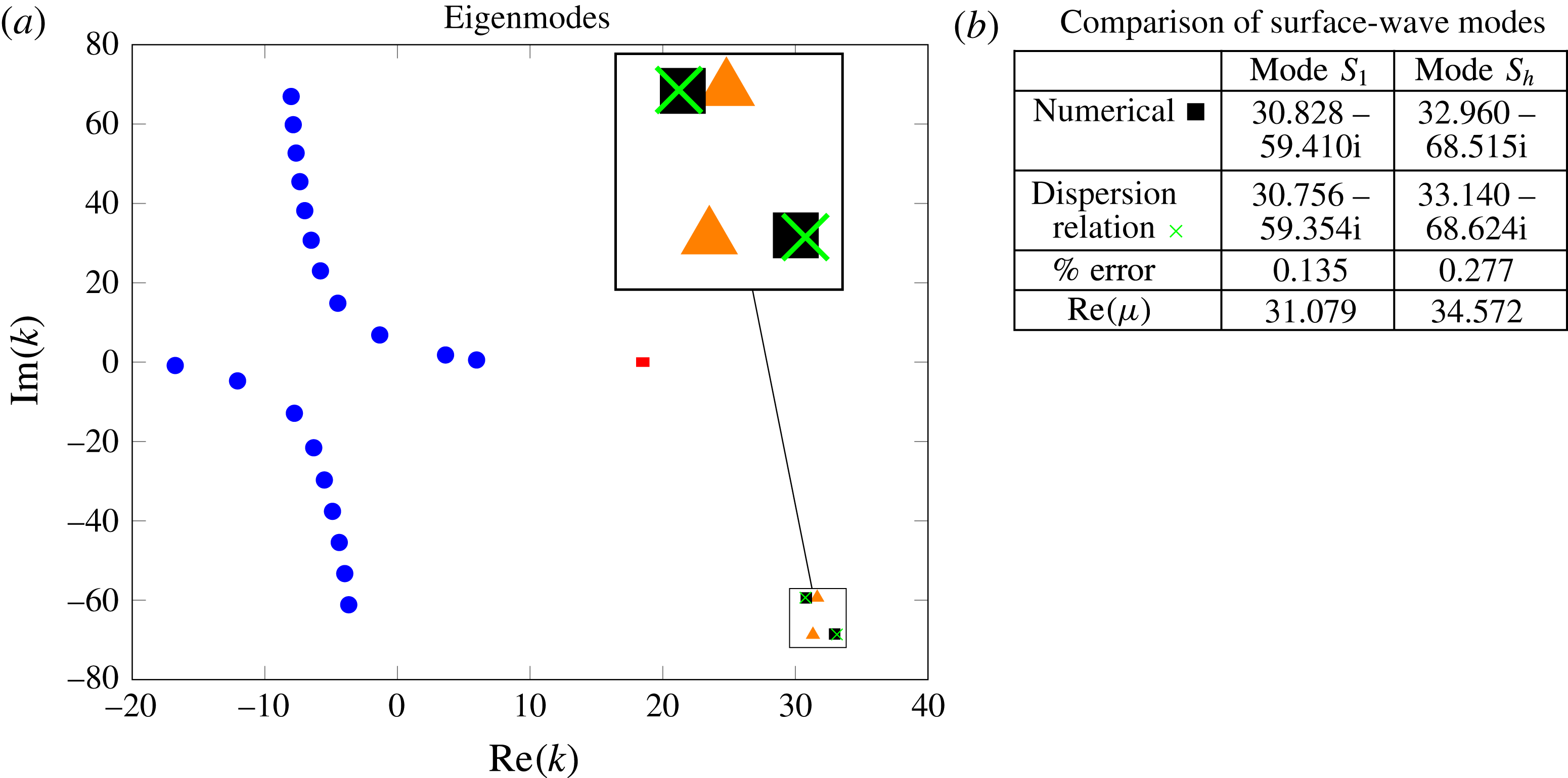
Plot of the numerical acoustic modes (blue circles), numerical surface-wave modes (black squares: corrected Myers’, orange triangles: original Myers’), the dispersion relation surface-wave modes (green crosses: corrected Myers’) and critical layer (red). The parameters are
 $M_{x}=0.5$
,
 $M_{\unicode[STIX]{x1D703}}=0.5$
,
 $h=0.5$
,
 $\unicode[STIX]{x1D714}=10$
,
 $m=1$
and
 $Z(\unicode[STIX]{x1D714})=1.6-0.08\text{i}\unicode[STIX]{x1D714}+6\text{i}/\unicode[STIX]{x1D714}$
.

The numerical modes (blue circles for acoustic modes, black squares for surface-wave modes) for the corrected Myers boundary condition are plotted in figure 7(a), together with the surface-wave modes predicted by the analytical dispersion relation (green crosses) using (6.8) and (6.9). Two solutions to the dispersion relation with
 $\text{Re}(\unicode[STIX]{x1D707})\gg 1$
are found, one at each duct wall. Two further solutions are found with
 $\text{Re}(\unicode[STIX]{x1D707})\approx 0.15$
for both, and the nearest numerical modes to these lie in the line of acoustic modes. Thus these solutions are not localised waves close to the surface, and should not be considered as surface-wave modes in nature. A comparison between the numerical modes and the dispersion relation solutions is shown in figure 7(b): the relative error of the modes from the dispersion relation compared with the numerical modes is very small stressing the accuracy of the asymptotic model. Moreover for the two surface-wave modes very large values of
 $\text{Re}(\unicode[STIX]{x1D707})$
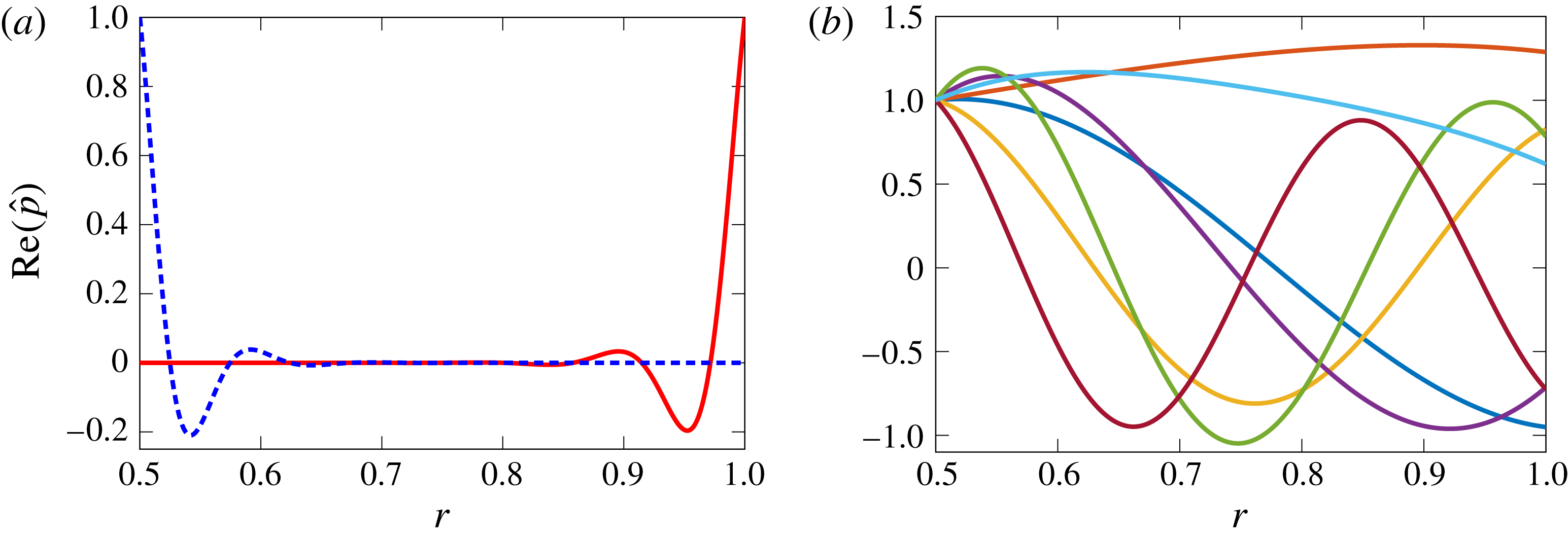
are obtained, showing rapid exponential decay. This is confirmed in figure 8(a) showing the eigenfunctions from the two surface waves in figure 7. The rapid exponential decay along with a small amount of oscillation can be clearly seen, as predicted by the asymptotic method due to the large values of
 $\text{Re}(\unicode[STIX]{x1D707})$
. The surface-wave eigenfunctions at the inner and outer wall also appear relatively symmetric, although they are not exactly. Comparing with the eigenfunctions for the seven most cut-on acoustic eigenmodes shown in figure 8(b) demonstrates that the eigenfunctions from the surface waves are very distinctive and localised around the duct walls.
Plot of real part of eigenfunctions (normalised so that
 $\hat{p}(r)=1$
at one duct wall) for the modes from figure 7. (a) Surface-wave modes:
 $k=30.828{-}59.410\text{i}$
(red),
 $k=32.960{-}68.515\text{i}$
(blue, dashed). (b) Seven most cut-on acoustic modes:
 $k=3.62+1.80\text{i}$
(blue),
 $k=5.97+0.54\text{i}$
(orange),
 $k=-1.34+6.85\text{i}$
(yellow),
 $k=-12.06-4.73\text{i}$
(purple),
 $k=-7.77-12.89\text{i}$
(green),
 $k=-4.50+14.85\text{i}$
(sky-blue),
 $k=-16.76-0.85\text{i}$
(brown).

In figure 7(a) a comparison between the surface-wave modes using the corrected Myers boundary condition (black squares) and the original Myers boundary condition (orange triangles) is also seen. Much more difference in the surface-wave modes is obtained for the two boundary conditions than was found for the acoustic modes. Indeed in figure 7(a) the acoustic modes from the two boundary conditions can hardly be distinguished, as already observed in figures 5 and 6. In fact the distance between the surface-wave modes for the different boundary conditions is
 $\unicode[STIX]{x0394}k=0.83$
for the upper left surface-wave mode (
 $S_{1}$
), and
 $\unicode[STIX]{x0394}k=1.64$
for the lower right surface-wave mode (
 $S_{h}$
) which corresponds to relative difference of 1.24 % and 2.16 % respectively. The distances between the acoustic modes for the two boundary conditions is of the order of
 $\unicode[STIX]{x0394}k=0.01$
.
If the surface waves were to be considered at much lower frequency, like in figure 2, then even more of a difference in the surface-wave modes would be seen for the two boundary conditions. For the corrected Myers boundary condition and the same parameters as figure 2, a surface-wave mode is numerically given by
 $k=5.7379-2.4009\text{i}$
, which is to the right of the critical layer (which has end points
 $k=1.8$
and
 $k=2.8$
). Note that this mode has
 $\text{Re}(\unicode[STIX]{x1D707})\approx 6.3$
, so while it decays exponentially, its variation is relatively slow. If the original Myers boundary condition is used, then the surface wave would be given by
 $k=3.9108-3.2616\text{i}$
, which is a significant distance away, with a relative error of approximately 32 % compared with using the correct boundary condition.
The numerical surface modes in figure 7 have been calculated for an infinitely thin boundary layer, and are now compared to the true surface modes for a fully resolved exponential boundary layer as the boundary-layer thickness tends to zero, as in § 5.1 for the acoustic modes. The difficulty here is that the dispersion relation given by (6.9) assumes the mean flow to vary more slowly than the surface-wave eigenfunction, which is no longer valid when resolving a thin boundary layer, and so we have no approximation for the surface modes with the boundary layer resolved. Therefore, we have started with a very thin boundary layer where the surfaces modes are known to be close to the numerical solutions in figure 7, and have gradually increased the boundary-layer thickness.
In table 4 two surface modes (one for each wall) are considered for different boundary layers thicknesses, as well as for an infinitely thin boundary layer with the corrected Myers and the original Myers boundary condition. For
 $\unicode[STIX]{x1D6FC}>8000$
(where
 $L_{\unicode[STIX]{x1D6FC}}$
is the exponential envelope) resolving the very thin boundary layer becomes difficult, while for
 $\unicode[STIX]{x1D6FC}<1600$
the surface modes start moving very fast and become hard to track. Even though such restrictions prevent any definite conclusions, the corrected Myers boundary condition appears to be more likely the limit case as the boundary-layer thickness tends to zero than the original Myers boundary condition.





6.3.2 Number of surface-wave modes
Next, how the number of surface-wave modes varies with the impedance is considered. In Brambley & Peake (Reference Brambley and Peake2006, figure 2), this was dealt with for a range of parameters for uniform axial flow and no swirl. A more realistic flow is taken here instead, and the SDT flow (without a boundary layer) from figure 4 is used. For reference the flow parameters at the duct walls are
 $U_{x}(h)=0.3188$
,
 $U_{\unicode[STIX]{x1D703}}(h)=-0.2869$
,
 $U_{x}(1)=0.2803$
and
 $U_{\unicode[STIX]{x1D703}}(1)=-0.2658$
. For this turbofan case, the variation of the number of surface-wave modes from the dispersion relation which satisfy
 $\text{Re}(\unicode[STIX]{x1D707})\gg 1$
with the impedance
 $Z$
is studied. This will serve as a proxy for the exact number of numerical surface-wave modes, which would be much more computationally expensive.
Because of the more complicated flow, several parameters are expected to control the behaviour of the number of surface-wave modes. A variety of different flows, frequencies and azimuthal numbers could be considered, but for simplicity just a single case (
 $m=1$
,
 $\unicode[STIX]{x1D714}=15$
and SDT flow) is considered to illustrate some of the possible behaviours. To be able to determine the number of surface-wave modes, the range over which
 $\text{Re}(\unicode[STIX]{x1D707})$
satisfies
 $\text{Re}(\unicode[STIX]{x1D707})\gg 1$
needs to be specified. In Brambley & Peake (Reference Brambley and Peake2006) the number of surface-wave modes with
 $\text{Re}(\unicode[STIX]{x1D707})>0$
was considered.
 $\text{Re}(\unicode[STIX]{x1D707})>5$
is used instead here for the classification of surface waves, as it is a more realistic guide as to whether a mode is acoustic or a surface wave.
Plot of the lines
 $\text{Re}(\unicode[STIX]{x1D707})=5$
mapped into the
 $Z$
plane. In each region there are a different number of surface-wave modes with
 $\text{Re}(\unicode[STIX]{x1D707})>5$
. The regions have been labelled with the number of surface-wave modes and coloured differently. The parameters are SDT flow,
 $m=1$
and
 $\unicode[STIX]{x1D714}=15$
.

In figure 9 the lines
 $\text{Re}(\unicode[STIX]{x1D707})=5$
mapped into the
 $Z$
plane are plotted. These lines correspond to where a surface wave has exactly
 $\text{Re}(\unicode[STIX]{x1D707})=5$
, and thus crossing one of these lines changes the number of surface-wave modes. These lines were generated numerically, since unlike the case of uniform flow in Brambley & Peake (Reference Brambley and Peake2006), an analytical expression for these lines cannot be obtained.
It is clear from figure 9 that there are no surface waves at either wall for an impedance with
 $\operatorname{Im}(Z)<-1$
, which corresponds to region zero in both images (in green). A total of exactly eight surface-wave modes can also be found, with four at each wall (region IV, shown in blue), by choosing an impedance of say
 $Z=1.5\text{i}$
. Any combination between zero and eight surface-wave modes in total at both walls can also be produced by carefully choosing the impedance and consequently moving to the other zones of the map (1 surface-wave mode per wall in the grey zone, 2 in the yellow zone and 3 in the red zone). The impedance chosen in § 5,
 $Z=2.55+1.5\text{i}$
, is marked with a red cross, and lies in region II (yellow) at both duct walls, corresponding to two surface waves at each wall. The surface waves at the outer wall can be numerically calculated as
 $k=380.08-417.45\text{i}$
and
 $k=-154.12+474.89\text{i}$
, while the inner wall surface waves are given by
 $k=317.05-375.60\text{i}$
and
 $k=-112.25+378.88\text{i}$
. Thus, it is clear why they do not appear in figure 5.
Finally, it should be noted that if the original Myers boundary condition were to be used instead of the corrected Myers boundary condition, this would have the effect of shifting figure 9 up or down. Figure 9(a) would be shifted down by
 $\unicode[STIX]{x1D70C}_{0}^{nbl}(1)M_{\unicode[STIX]{x1D703},1}^{2}/\unicode[STIX]{x1D714}$
to get the result for the original Myers boundary condition, and figure 9(b) would be shifted up by
 $\unicode[STIX]{x1D70C}_{0}^{nbl}(h)M_{\unicode[STIX]{x1D703},h}^{2}/(h\unicode[STIX]{x1D714})$
. Thus, it is clear that depending on the amount of shift (especially at low frequencies) the number of surface-wave modes would be different for the two boundary conditions. However, this is because an exact criterion for surface waves,
 $\text{Re}(\unicode[STIX]{x1D707})>5$
, has been introduced. In reality the same number of surface-wave modes exists, but some have changed their exponential decay and are closer to becoming acoustic modes.
The procedure for finding surface waves by tracking modes as
 $Z$
is varied, as described in Rienstra (Reference Rienstra2003, § 6) is still valid in swirling flow (at least for this case). For this procedure, an initial impedance is selected in the zero region (in green) in figure 9 where no surface waves at either wall are to be found, and where all the modes are consequently acoustic modes. It is relatively easy to calculate these modes numerically. The impedance can then be slowly varied to the true value being considered, which will probably involve crossing contours in figure 9. As these contours are approached, surface-wave modes will emerge from the line of acoustic modes, which can then be traced as the impedance further varies. Using this method, the need for initial guesses at the wavenumbers of possible surface waves could be avoided completely.
6.4 Stability of surface waves
Briggs–Bers contours as the frequency is increased from
 $\unicode[STIX]{x1D714}=10$
to
 $\unicode[STIX]{x1D714}=10+8\text{i}$
. The blue/red circles indicate the position at
 $\unicode[STIX]{x1D714}=10$
, green/orange crosses at
 $\unicode[STIX]{x1D714}=10+8\text{i}$
, and the black contour are the paths between. The other parameters are
 $M_{x}=0.5$
,
 $M_{\unicode[STIX]{x1D703}}=0.5$
,
 $h=0.5$
,
 $m=1$
and
 $Z(\unicode[STIX]{x1D714})=1.6-0.08\text{i}\unicode[STIX]{x1D714}+6\text{i}/\unicode[STIX]{x1D714}$
.

The stability of the surface waves is now considered. To begin with, the Briggs–Bers (Briggs Reference Briggs1964; Bers Reference Bers1983; Brambley Reference Brambley2009) contours are plotted for figure 7(a), which show the stability of the modes. These are traces of the eigenmodes as the imaginary part of frequency is increased from zero (in Brambley (Reference Brambley2009) it is decreased from zero due to the different sign of
 $\text{e}^{-\text{i}\unicode[STIX]{x1D714}t}$
). In figure 10 these traces are shown in black as the frequency is increased from
 $\unicode[STIX]{x1D714}=10$
to
 $\unicode[STIX]{x1D714}=10+8\text{i}$
, with the blue circles (acoustic modes) and red circles (surface-wave modes) showing the initial positions at
 $\unicode[STIX]{x1D714}=10$
, and green crosses (acoustic modes) and orange crosses (surface-wave modes) showing the position at
 $\unicode[STIX]{x1D714}=10+8\text{i}$
. The other parameters are the same as in figure 7(a).
The acoustic modes are seen not to move that much as the imaginary part of
 $\unicode[STIX]{x1D714}$
is varied. For each frequency exactly one surface wave per wall is found. These were obtained by using the dispersion relations given by (6.8) and (6.9) as starting guesses for calculating these surface-wave modes numerically. As the imaginary part of the frequency is increased, the surface-wave modes move to the right and down, and do not cross the real axis. Therefore these surface-wave modes are stable.
Briggs–Bers contours as the frequency is increased from
 $\unicode[STIX]{x1D714}=10$
to
 $\unicode[STIX]{x1D714}=10+20\text{i}$
. The blue/red circles indicate the position at
 $\unicode[STIX]{x1D714}=10$
, green/orange crosses at
 $\unicode[STIX]{x1D714}=10+20\text{i}$
, and the black contours are the paths between. The other parameters are
 $M_{x}=0.8$
,
 $M_{\unicode[STIX]{x1D703}}=0.5$
,
 $h=0.5$
,
 $m=1$
and
 $Z(\unicode[STIX]{x1D714})=1.6-0.08\text{i}\unicode[STIX]{x1D714}+6\text{i}/\unicode[STIX]{x1D714}$
.

For a more interesting case concerning unstable surface-wave modes, a flow with
 $U_{x}(r)=0.8$
is considered instead, with the other parameters unchanged. The Briggs–Bers contours are plotted in figure 11 for
 $\unicode[STIX]{x1D714}=10$
to
 $\unicode[STIX]{x1D714}=10+20\text{i}$
. The downstream acoustic modes are again seen not to move that much as the imaginary part of
 $\unicode[STIX]{x1D714}$
is varied, although the upstream acoustic modes move more than in the previous case. We also note that the two downstream acoustic modes with the largest imaginary part in figure 11 have more interesting behaviour than their counterparts, with the trajectory of one of them forming a loop.
Initially, there is one surface wave per wall, labelled
 $S_{1}$
and
 $S_{h}$
, and both have negative imaginary axial wavenumbers
 $k$
. They move considerably as the imaginary part of frequency is varied, with both crossing the real axis and moving into the upper half-plane. The surface mode
 $S_{1}$
crosses the real axis for
 $16<\operatorname{Im}(\unicode[STIX]{x1D714})<17$
, while the surface mode
 $S_{h}$
crosses shortly afterwards when
 $18<\operatorname{Im}(\unicode[STIX]{x1D714})<19$
. If the imaginary part of frequency was further increased then these surface-wave modes would continue to move upwards, with both crossing the line
 $\operatorname{Im}(k)=100$
at around
 $\operatorname{Im}(\unicode[STIX]{x1D714})\approx 58$
. Owing to their presence in the upper half-plane for sufficiently large
 $\operatorname{Im}(\unicode[STIX]{x1D714})$
, these surface waves are found to be convectively unstable.
Thus, each wall is found to support up to one convectively unstable surface wave for swirling flow. Furthermore, at each wall this unstable mode travels downstream. This is the same situation as in the non-swirling case. It is entirely possible and reasonable that we get a stable surface mode at one wall, and an unstable surface mode at the other wall. Whilst we cannot rule out the possibility that more than one surface mode per wall is unstable for some set of parameters, for all the realistic parameters we have calculated at most one instability per wall was present.
The stability of the SDT flow from figure 4 is finally considered but now with
 $\unicode[STIX]{x1D714}=10$
,
 $m=-5$
,
 $h=0.5$
and the mass–spring–damper impedance. Two surface modes are found that have negative axial wavenumber for
 $\unicode[STIX]{x1D714}=10$
, and as the imaginary part of frequency is increased they move further from the real line, with the negative imaginary part of the axial wavenumber increasing. The Briggs-Bers contours would look very similar to figure 10, and the SDT flow would be stable. If a frequency of
 $\unicode[STIX]{x1D714}=3$
was considered instead for the SDT flow with the other parameters unchanged then two surface modes would be found to cross the real axis as the imaginary part of frequency is increased and hence the flow is unstable.
6.4.1 Temporal stability of the surface waves
Finally, the temporal stability of the surface waves is considered. Khamis & Brambley (Reference Khamis and Brambley2016) considered the temporal stability of the unstable surface wave for uniform axial non-swirling flow using three different boundary conditions: the Myers, modified Myers and second-order boundary condition. It was shown that using the Myers boundary condition gives an unbounded temporal growth rate and makes the problem ill posed, while using the modified Myers or second-order boundary condition gives a bounded growth rate, with the second-order boundary condition more closely replicating the numerics.
The growth rate of the corrected Myers boundary condition in the presence of swirl is of interest here. The simple swirling flow from figure 11 is considered, and the frequency
 $\unicode[STIX]{x1D714}$
of the unstable surface wave is solved for as
 $k$
is varied with
 $k$
real. The unstable surface wave
 $S_{h}$
lies on the real line at
 $k=109.89$
,
 $\unicode[STIX]{x1D714}=10+18.42\text{i}$
, and the surface wave
 $S_{1}$
lies on the real line at
 $k=89.48$
,
 $\unicode[STIX]{x1D714}=10+16.75\text{i}$
. Instead of solving the system in (4.1) for the axial wavenumber
 $k$
with
 $\unicode[STIX]{x1D714}$
given, the inverse problem is considered with wavenumber
 $k$
given and the eigenmode
 $\unicode[STIX]{x1D714}$
to be found. The resulting
 $k$
versus growth rate,
 $\operatorname{Im}(\unicode[STIX]{x1D714})$
, is plotted in figure 12(a), along with a plot of
 $\operatorname{Im}(\unicode[STIX]{x1D714})$
against
 $\text{Re}(\unicode[STIX]{x1D714})$
in figure 12(b). These lines correspond to surface wave transitioning from spatially stable to spatially unstable, as their related axial wavenumber crosses the real axis in the complex
 $k$
-plane. As an example, the points where the surface-wave modes cross the real axis in figure 11 are marked with circles in figure 12, and correspond to surface waves becoming unstable for this specific set of parameters. Note also that as
 $k$
or
 $\text{Re}(\unicode[STIX]{x1D714})$
are decreased, the surface-wave modes get closer together as seen in figure 12(b).
Trajectory of the two surface-wave modes
 $S_{h}$
and
 $S_{1}$
from figure 11 as
 $k$
is varied along the real line. Plot of (a) growth rate
 $\operatorname{Im}(\unicode[STIX]{x1D714})$
versus
 $k$
and (b)
 $\text{Re}(\unicode[STIX]{x1D714})$
versus
 $\operatorname{Im}(\unicode[STIX]{x1D714})$
.

It appears that, for both surface waves, the growth rate
 $\operatorname{Im}(\unicode[STIX]{x1D714})$
is unbounded as both
 $k$
and
 $\text{Re}(\unicode[STIX]{x1D714})$
increase, suggesting that the corrected Myers boundary condition is ill posed in swirling flow, as in the axial flow case. Therefore, the present stability analysis is not strictly correct and a well-posed boundary condition should be considered instead. Such a model is developed in Mathews et al. (Reference Mathews, Masson, Moreau and Posson2018).
7 Conclusion and future work
In the present study, a generalisation of the Myers boundary condition has been developed in an annular duct with swirl, both for the inner wall and for the outer wall. It has been shown that the classical Myers boundary condition is not the correct limit when an infinitely thin boundary layer is considered at the walls in the presence of swirl. Indeed, centrifugal effects modify the boundary condition by introducing an extra spring-like term to the effective impedance. The new boundary condition has the correct linear error behaviour when the boundary-layer thickness tends to zero. While the spring-like correction term is inversely proportional to frequency, it nevertheless remains the same magnitude as any spring-like terms within the wall impedance which are typically not neglected even at high frequencies, and it is shown that neglecting this extra term can lead to significant error in the low frequency range. The corrected boundary condition has been tested with a flow profile representative of a realistic turbofan bypass. If a typical boundary-layer thickness is considered, results are still far from the reference numerical solution. To improve the prediction, the boundary condition should be further expanded to first order with respect to the boundary-layer thickness. This method is presented in Mathews et al. (Reference Mathews, Masson, Moreau and Posson2018).
A dispersion relation for the surface waves in swirling flow has been established which differs significantly from the dispersion relation in non-swirling flow. This new surface-wave dispersion relation may be used with the impedance given by the corrected Myers boundary condition to accurately predict surface waves in swirling flow. The dispersion relation is a polynomial of order four with respect to the axial wavenumber
 $k$
, meaning there are at most four surface waves per wall, as in the non-swirling case. If the swirl is set to zero, the surface-wave dispersion relation reduces to one asymptotically equivalent to that of Brambley & Peake (Reference Brambley and Peake2006).
The surface-wave dispersion relation has then been shown to accurately predict the location of the numerical surface waves for arbitrary swirling flow profiles. The choice of boundary condition has been found to have a quite significant effect on the surface waves. Depending on the impedance of the duct walls, there can be between zero and eight surface waves in total over the inner and outer walls, and it is possible to use the dispersion relation to identify regions where a certain number of surface waves are present. Finally, the stability of the surface waves has been considered, and we found up to one unstable surface-wave modes per wall, as in the non-swirling case. Additionally, at least one of these unstable surface waves is found to be temporally unstable with an unbounded growth rate, rendering the corrected Myers boundary condition ill posed, as is the Myers boundary condition in the non-swirling case.
Although this paper only considered a homentropic base flow, the inclusion of entropy gradients in the base flow is certainly possible and is an area to be investigated in the future. This would lead to a different dispersion relation for the surface waves, although a similar method could still be used. Another aspect to be considered in the future would be the corrected Myers boundary condition in a curved duct, which would be more challenging. Another area of future work would be to consider perturbations in the time domain or with arbitrary axial and circumferential variance (rather than Fourier), for which the method in this paper can be readily applied.
Acknowledgements
A preliminary version (unreviewed) of the present work (Masson et al. Reference Masson, Mathews, Sanjose, Moreau and Posson2017) was presented as AIAA paper 2017-3385 at the 23rd AIAA/CEAS Aeroacoustic Conference in Denver (CO), USA, 5 June–9 June. The authors would like to thank Professor M. Roger from École Centrale de Lyon as well as Dr D. Khamis and Professor N. Peake from the University of Cambridge for the interesting conversations about this topic and their precious advice. They are also grateful to T. Nodé-Langlois from Airbus for having provided the RANS data for the SDT test case. J.R.M. was funded by ENOVAL, grant number 604999. V.M. was funded by Airbus through the Industrial Chair in Aeroacoustics at Université de Sherbrooke. He performed the present work in the Laboratoire de Mécanique des Fluides et d’Acoustique of École Centrale de Lyon, within the framework of the Labex CeLyA of the Université de Lyon, within the programme ‘Investissements d’Avenir’ (ANR-10- LABX-0060/ANR-11-IDEX-0007) operated by the French National Research Agency (ANR).
Appendix A
In (4.1) the matrix
 $\unicode[STIX]{x1D63C}$
is given by
 $$\begin{eqnarray}\displaystyle & & \displaystyle \unicode[STIX]{x1D63C}=\left(\begin{array}{@{}cccc@{}}{\displaystyle \frac{\bar{\unicode[STIX]{x1D714}}}{U_{x}}} & -{\displaystyle \frac{2U_{\unicode[STIX]{x1D703}}}{rU_{x}}} & 0 & -{\displaystyle \frac{\text{i}U_{\unicode[STIX]{x1D703}}^{2}}{rc_{0}^{2}\unicode[STIX]{x1D70C}_{0}U_{x}}}+{\displaystyle \frac{\text{i}}{U_{x}\unicode[STIX]{x1D70C}_{0}}}{\displaystyle \frac{\text{d}}{\text{d}r}}\\[12.0pt] -\left({\displaystyle \frac{U_{\unicode[STIX]{x1D703}}}{rU_{x}}}+{\displaystyle \frac{U_{\unicode[STIX]{x1D703}}^{\prime }}{U_{x}}}\right) & {\displaystyle \frac{\bar{\unicode[STIX]{x1D714}}}{U_{x}}} & 0 & -{\displaystyle \frac{\text{i}m}{r\unicode[STIX]{x1D70C}_{0}U_{x}}}\\[12.0pt] -{\displaystyle \frac{1}{\unicode[STIX]{x1D6FD}^{2}}}\left({\displaystyle \frac{1}{r}}+{\displaystyle \frac{\unicode[STIX]{x1D70C}_{0}^{\prime }}{\unicode[STIX]{x1D70C}_{0}}}-{\displaystyle \frac{U_{x}U_{x}^{\prime }}{c_{0}^{2}}}\right)-{\displaystyle \frac{1}{\unicode[STIX]{x1D6FD}^{2}}}{\displaystyle \frac{\text{d}}{\text{d}r}} & -{\displaystyle \frac{m}{\unicode[STIX]{x1D6FD}^{2}r}} & -{\displaystyle \frac{\bar{\unicode[STIX]{x1D714}}U_{x}}{\unicode[STIX]{x1D6FD}^{2}c_{0}^{2}}} & {\displaystyle \frac{\text{i}\bar{\unicode[STIX]{x1D714}}}{\unicode[STIX]{x1D6FD}^{2}\unicode[STIX]{x1D70C}_{0}c_{0}^{2}}}\\[12.0pt] {\displaystyle \frac{\text{i}}{\unicode[STIX]{x1D6FD}^{2}}}\left(\unicode[STIX]{x1D70C}_{0}U_{x}^{\prime }-{\displaystyle \frac{U_{x}\unicode[STIX]{x1D70C}_{0}}{r}}-U_{x}\unicode[STIX]{x1D70C}_{0}^{\prime }\right)-{\displaystyle \frac{\text{i}\unicode[STIX]{x1D70C}_{0}U_{x}}{\unicode[STIX]{x1D6FD}^{2}}}{\displaystyle \frac{\text{d}}{\text{d}r}} & -{\displaystyle \frac{\text{i}m\unicode[STIX]{x1D70C}_{0}U_{x}}{r\unicode[STIX]{x1D6FD}^{2}}} & -{\displaystyle \frac{\text{i}\unicode[STIX]{x1D70C}_{0}\bar{\unicode[STIX]{x1D714}}}{\unicode[STIX]{x1D6FD}^{2}}} & -{\displaystyle \frac{\bar{\unicode[STIX]{x1D714}}U_{x}}{\unicode[STIX]{x1D6FD}^{2}c_{0}^{2}}}\end{array}\right),\nonumber\\ \displaystyle & & \displaystyle\end{eqnarray}$$
where
 $\bar{\unicode[STIX]{x1D714}}$
is the shifted frequency defined by
 $\bar{\unicode[STIX]{x1D714}}=\unicode[STIX]{x1D714}-mU_{\unicode[STIX]{x1D703}}/r$
,
 $\unicode[STIX]{x1D6FD}$
is the local compressibility factor defined by
 $$\begin{eqnarray}\displaystyle \unicode[STIX]{x1D6FD}(r)=\sqrt{1-{\displaystyle \frac{U_{x}^{2}(r)}{c_{0}^{2}(r)}}}, & & \displaystyle\end{eqnarray}$$
and where the superscript
 $^{\prime }$
denotes the derivative with respect to
 $r$
for conciseness. The matrix
 $\unicode[STIX]{x1D63D}$
is the identity matrix everywhere but on the first and the last lines where the boundary conditions are applied.