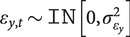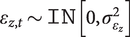


1. Introduction
One characteristic of both the Covid-19 data on confirmed cases and deaths and macroeconomic data over the pandemic is their inherent nonstationarity. The Covid-19 data exhibit continually changing trends, with explosive roots in some periods, and they are also subject to abrupt shifts. Every aspect of the distribution is changing over time, as can be seen in figure 1, which records total and new cases and deaths for the UK, with data from the start of the pandemic to 14 January 2021. Panels (e) and (f) highlight how the distributions are shifting over time. Added to the problem of nonstationary data is the compounding effect of the nonstationarity of the reporting process. There are reporting delays, changing definitions and data errors. For example, the expansion of infection and antibody testing, the sudden inclusion of care home cases for the UK, corrections for previous errors in reporting leading to negative numbers reported for cases for some days, omitting rows of data due to the use of out-dated Excel spreadsheets and lags in data releases, especially at the weekend, generating weekly changing ‘seasonality’. The nonstationarity of the data interacts with the nonstationarity of the reporting process and the changing seasonal pattern, which requires highly adaptive forecasting methods. Macroeconomic data are also subject to changing stochastic trends, abrupt distributional shifts, structural breaks and outliers, measurement errors, data revisions and seasonality, so it is natural to see if the same forecasting methods could be useful to both Covid-19 and macroeconomic data.
(Colour online) Panel (a): UK total confirmed cases. Panel (b): UK total deaths. Panel (c): UK confirmed cases with smoothed trend. Panel (d): UK new deaths with smoothed trend. Panel (e): densities for new cases averaged over 3-month intervals. Panel (f): densities for new deaths averaged over 3-month intervals

There is a two-way interaction between the pandemic and the economy. As confirmed cases and deaths grew exponentially, public health policy led to the first lockdown, resulting in a substantial fall in output, and following with a lag, a fall in cases and deaths, leading in turn to a relaxation of lockdown. Large extensions in testing detected more cases, as many individuals were asymptomatic, and cases began increasing rapidly again after educational institutions reopened, indeed far exceeding the initial levels. Although the NHS remained under considerable strain, Covid-19 death rates dropped sharply from improved procedures, probably leading some individuals to take greater risks, especially those whose livelihoods depended on working, and younger ages, further spreading the virus. This resulted in a second lockdown and further changes in economic policy. The new B117 variant led to a further explosion of cases and deaths, resulting in a third lockdown. Given the close interactions between public health policy and its impact on the economy, it should not come as a surprise that forecasting devices that are successful in one arena may also be valuable in the other.
Ideally, the health and economic systems would be jointly forecast, with forecasts of Covid-19 cases and deaths used to predict policy responses to the health crisis including lockdowns. This, in turn, predicts an economic response to the lockdown, namely rising unemployment, which would predict a policy response such as furlough policies. In practice, this joint system is too challenging to model to produce accurate forecasts at longer horizons. The economic and health responses operate at different frequencies. We produce 7-day ahead forecasts for Covid-19, which gives sufficient time to ensure ICU capacity, healthcare availability and so on, but we produce 1–3-month ahead forecasts for unemployment which are less timely as the data are only available with a substantial lag. Tying together the health and economic systems is difficult, but there are many commonalities in both the data and forecasting procedures that we discuss below.
There are two dominant approaches to forecasting that can be applied to health and economic data: structural models, including epidemiological models and, for example, dynamic stochastic general equilibrium models in economics, and time-series models, which could include autoregressive models, Theta (Assimakopoulos and Nikolopoulos, Reference Assimakopoulos and Nikolopoulos2000), Cardt (Castle et al., Reference Castle, Doornik and Hendry2021) and growth curves (Harvey and Kattuman, Reference Harvey and Kattuman2020). While structural and statistical models have different underlying assumptions and different ways of using past data, they can both be informative. Neither approach captures the true underlying data generating process (DGP) of the disease transmission mechanism, which depends on a myriad of factors including host, social, environmental and policy variables, resulting in a far too complex process to model. Instead, both rely on simplifying assumptions.
Epidemiological models, like structural models in economics, have a sound theoretical basis and many useful applications. Structural models are invaluable to understanding what is going on, but at the same time there is a history of simple data-based devices out-forecasting those structural models, not just in economics but in many different disciplines. One of the reasons for these forecast results is that there are shifts in the distribution of the data that lead to systematically poor forecasts. This is because models tend to have a built-in equilibrium to which they revert, but if the data have shifted (as seen in figure 1), the forecasts will try to return to the wrong equilibrium. From their taxonomy of all sources of forecast errors, Clements and Hendry (Reference Clements and Hendry1998) show that forecast failure, where outcomes systematically lie well outside interval forecasts, is primarily due to unanticipated shifts. As they are unanticipated, large forecast errors are relatively common. However, systematic forecast failure arises from not adjusting to the shift after it has occurred. In this paper, we contrast statistical forecasting methods that adapt rapidly, relying purely on the recent past data capturing how it has evolved and shifted to predict what will happen next, to more structural models based on epidemiology or economic theory.
Adaptive forecasting devices rapidly adjust to the latest information in the data, handling both stochastic trends and abrupt shifts. In Section 2, we present a statistical forecasting device (Cardt; see Castle et al., Reference Castle, Doornik and Hendry2021) that is highly adaptive and has been shown to work well in forecasting the 100,000 time series of varying frequency and sample length in the M4 competition (see Makridakis et al., Reference Makridakis, Spiliotis and Assimakopoulos2020). Section 3 applies that forecasting device to short-term forecasts of Covid-19 confirmed cases and deaths (see also Doornik et al., Reference Doornik, Castle and Hendry2020b, Reference Doornik, Castle and Hendry2020c), evaluating these forecasts against published forecasts from epidemiological models. Section 4 forecasts UK aggregate unemployment, comparing our statistical forecasts to those from a more structural congruent econometric model, before Section 5 concludes.
2. An adaptive statistical forecasting device
To forecast Covid-19 cases and deaths, we begin by decomposing the data into a trend, seasonal and irregular component, and then forecast the components separately before aggregating. The forecasts for the trend and irregular components are computed using a statistical device we have developed for short-term forecasting called the Calibrated Average of Rho (
 $ \rho $
), Delta (
 $ \delta $
) and THIMA, or Cardt for short (see Castle et al., Reference Castle, Doornik and Hendry2021). It is a modified version of the forecasting device used in our submission for the M4 competition (Makridakis et al., Reference Makridakis, Spiliotis and Assimakopoulos2020) described in Doornik et al. (Reference Doornik, Castle and Hendry2020a). The seasonal component is extrapolated from the most recent estimates of the seasonal pattern. For the unemployment forecasts, we apply Cardt directly to the unemployment rate data rather than undertaking an initial decomposition, as the data are less messy owing to the estimates being reported as 3-month averages. The decomposition is outlined in Section 2.1, and the Cardt forecast device is described in Section 2.2.
2.1. Decomposing Covid-19 data into a trend, seasonal and irregular component
Define
 $ {I}_t $
as the cumulative number of positive tests and
 $ {i}_t $
for the daily number of positive tests, where
 $ {i}_t=\Delta {I}_t $
, and equivalently, the cumulative number of deaths is
 $ {D}_t $
, and the daily count is
 $ {d}_t=\Delta {D}_t $
, where we let
 $ {Y}_t $
denote
 $ {I}_t $
or
 $ {D}_t $
. Our forecasting models are for the logarithm of
 $ {Y}_t $
, adding 1 to allow for a zero count at the beginning of the pandemic. The resulting decomposition into trend
 $ {\hat{\mu}}_t $
, seasonal
 $ {\hat{\gamma}}_t $
and remainder
 $ {\hat{\varepsilon}}_t $
is
 $$ \log \left({Y}_t+1\right)=\log {\hat{\mu}}_t+\log {\hat{\gamma}}_t+{\hat{\varepsilon}}_t, $$
which is transformed back using
 $ {\hat{u}}_t=\exp \left({\hat{\varepsilon}}_t\right) $
:
 $$ {Y}_t={\hat{\mu}}_t{\hat{\gamma}}_t{\hat{u}}_t-1=\left[{\hat{\mu}}_t-1\right]{\hat{\gamma}}_t{\hat{u}}_t+\left[{\hat{\gamma}}_t{\hat{u}}_t-1\right]\approx \left[{\hat{\mu}}_t-1\right]{\hat{\gamma}}_t{\hat{\mu}}_t={\hat{Y}}_t{\hat{\gamma}}_t{\hat{u}}_t. $$
Both
 $ {\hat{\gamma}}_t $
and
 $ {\hat{u}}_t $
have an expectation of one and are uncorrelated.
The decomposition is obtained by taking moving windows of the data and saturating these by segments of linear trends, denoted trend indicator saturation (TIS; Castle et al., Reference Castle, Doornik, Hendry and Pretis2019). The changing seasonality is modelled by including six indicator variables for 6 days of the week and both a weekly sine and cosine wave, and a half-weekly sine and cosine wave. Despite redundancy, these can all be included initially as selection is applied. Sparsity is obtained by selecting the broken trends and seasonal components that are significant at tight significance levels using the machine learning tree-search algorithm, Autometrics (Doornik, Reference Doornik, Castle and Shephard2009). An estimate of the unobserved flexible trend and unobserved changing seasonal pattern is obtained by taking the average of the fitted values for each observation across all windows that include that observation. The remainder is the difference between the actual observation and the estimated trend and seasonal component.
2.2. The Cardt forecasting device
The trend and remainder terms are forecast separately using Cardt, and recombined, adding in the seasonal component from the last observations at the seasonal frequency (e.g., the seasonal pattern from the last week of in-sample data for the daily Covid-19 data is extrapolated forwards) in a final forecast. Cardt is applied to the irregular component, as there may be some residual dynamics that are captured in the decomposition. The remainder is not a martingale-difference process.
To apply Cardt, three models are estimated including:
 $ \delta $
: Obtains estimates of the growth rate based on first differences, but is dampened by removing large values and allowing for seasonality.
 $ \rho $
: Estimates a simple autoregressive model with seasonality, forcing a unit root if the estimates are close to one and hence switching to a model in first differences with dampened mean.
THIMA: A trend-halved integrated moving average model, which consists of a dampened trend which is arbitrarily halved, together with an intercept correction estimated by a moving average model.
The arithmetic mean average of the three forecasts is computed. These forecasts are then calibrated by treating them as if they were observed, and a richer autoregressive model is estimated from the extended data series. The fitted values from this calibrated model give the final forecasts, undoing any transformations such as log and differencing. Higher orders of integration [e.g., I(2) and damped I(2)] can be allowed for when applying the methodology; Doornik et al. (Reference Doornik, Castle and Hendry2020b) provides further details.
The results from the M3 and M4 competition data, which include data of differing sample sizes, frequencies, category of data and degree of nonstationarity (both stochastic trends and abrupt shifts), suggest that the Cardt method forecasts well over short horizons. The method dampens trends and growth rates, which is important to avoid wild forecasts, averages across forecasts (which is a principle dating back to Bates and Granger, Reference Bates and Granger1969) and robustifies the forecasts to breaks in the data by ‘over-differencing’ (see Hendry, Reference Hendry2006). We next apply the forecasting method to Covid-19 cases and deaths in Section 3 and UK unemployment in Section 4.
3. Short-term forecasts of Covid-19 confirmed cases and deaths
We first published forecasts on 20 March 2020, forecasting 5 days ahead, and updating mostly every 2 days. The number of forecasts produced has since expanded to approximately 50 countries, 50 US states and over 300 Local Authority areas for England, forecasting 7 days ahead (see Doornik et al., Reference Doornik, Castle and Hendry2020b, Reference Doornik, Castle and Hendry2020c for details of how the forecasts are produced).Footnote 1 One important aspect of the algorithm is that it is automated, including downloading, sorting the data and forecasting. This enables a wide coverage and frequent updating of the forecasts.
Figure 2 shows an edited version of the forecasts for UK total cases and deaths for 14–20 January 2021, which were produced using data to 13 January 2020. The solid grey line records the actual data, obtained from the data repository for the 2019 Novel Coronavirus Visual Dashboard operated by the Johns Hopkins University Center for Systems Science and Engineering.Footnote
2 The dashed line records the trend decomposition
 $ \hat{\mu} $
. The red line is the forecast using the most recent data released. The grey lines are forecasts commencing from the last four data points, so commence with data conditioning only on actual outturns 4 days previously, 3 days previously and so on, but the forecasts are adjusted to match the last known observation. The average forecast is given in the black line. Big differences between the black and red lines enable us to monitor changes. For example, if policy is starting to be effective, we should see the red line based on most recent data deviate below the black line.
(Colour online) Forecasts for UK total confirmed cases [panel (a)] and total deaths [panel (b)] over 14 January to 20 January 2021
Source: www.doornik.com/COVID-19.

One important aspect of the forecasting method is its robustness to breaks. Figure 3 records the forecasts for total deaths in Italy early in the pandemic. In panel (a), the forecasts cover 6–12 March 2020, with the red line reporting the forecasts with 80 per cent uncertainty bands based on data available to 5 March 2020. The outturns are significantly higher after 2 days of forecasts, lying well outside the interval forecasts. The growth rate of cumulative deaths rose suddenly and quickly. An adaptive forecasting method needs to recover rapidly from these mistakes to avoid systematic failure. Moving 1 day forward in panel (b), the forecasts have updated and are now similar to the trajectory of the data, which was unknown at the time. The average forecast in black, using the last four observations as starting points, trails behind as expected given the shift, providing further evidence of when breaks occur in the data.
(Colour online) Forecasts for Italian total deaths over 6–12 March 2020 [panel (a)] and 7–13 March 2020 [panel (b)]
Source: www.doornik.com/COVID-19.

Prior to the second national lockdown for England, the policy approach had been to rank areas into tiers depending on the number of confirmed cases, with varying restrictions depending on the severity of cases within an area. This approach requires forecasts at a much finer resolution than the national level. Our statistical forecasting methods can be applied to highly disaggregated data such as data at the local authority level. The forecasts using the same methodology as that applied to the country level data are shown in figure 4, with the much darker shading in the right panel showing the huge increase in forecast cases in January 2021 relative to the previous summer.
(Colour online) Week ahead forecasts for confirmed cases per 100,000 by England Local Authority areas from 9 July 2020 (left panel) and 2 January 2021 (right panel)
Source: www.doornik.com/COVID-19.

3.1. Evaluation of statistical forecasts in comparison to epidemiological forecasts
We compare the evolution of the forecast performance of our statistical methods with those from the Los Alamos National Laboratory (LANL), which have been published twice a week since 5 April 2020, and forecasts from the Institute for Health Metrics and Evaluation (IHME), published since 25 March 2020 but not consistently.Footnote 3 The LANL forecasting model is not a full susceptible, infected and recovered epidemiological model, but is a modification of one in which they use a statistical model to capture the dynamics of the infection rate and then they map this to the reported data. They also produce uncertainty bands capturing model and measurement uncertainty.
Figure 5 records the forecast paths for the UK comparing our forecasts with those from LANL, with cases on the left panel and deaths on the right panel, up to November 2020. There are substantial revisions to both cases and deaths data. For confirmed cases, the UK data include results from both pillar 1 and pillar 2 testing. Pillar 1 testing includes those with a clinical need, and health and care workers, whereas pillar 2 testing is for the wider population. Up to 1 July, these data were collected separately meaning that people who had tested positive via both methods were counted twice. On 2 July, data for both pillars were combined, and around 30,000 duplicates were found and removed from the data, hence the revision to reported cases on 2 July. For the data on deaths, there was a large revision on 12 August. Deaths were redefined, so that a Covid-19-related death was recorded only if the individual had a positive test within the last 28 days. Previously, all deaths after a positive test were attributed to Covid-19. The data were then revised backwards. Time-series models have the advantage of adjusting to such data revisions rapidly, without the need for intercept adjustments as structural models would.
(Colour online) Forecast paths for UK, cases (left panel) and deaths (right panel), with our Cardt forecasts in red and LANL forecasts in blue
Source: www.doornik.com/COVID-19.

Table 1 evaluates the two forecast paths, reporting the mean absolute percentage error (MAPE) and root-mean-square percentage error (RMSPE), as well as the percentage of forecasts lying below the 10 per cent and above the 90 per cent quintiles, where
 $ F $
denotes our forecasts. Let
 $ {\hat{y}}_{j,T+h} $
denote a forecast at horizon
 $ h $
(where
 $ h $
spans
 $ 1-7 $
days ahead) from group
 $ j=1,\dots, J $
:
 $$ {\displaystyle \begin{array}{l}\hskip0.24em \mathrm{MAPE}=\frac{100}{J}\sum \limits_{j=1}^J\frac{\left|{y}_{j,T+h}-{\hat{y}}_{j,T+h}\right|}{y_{j,T+h}},\\ {}\mathrm{RMSPE}={\left[\frac{100}{J}\sum \limits_{j=1}^J{\left({y}_{j,T+h}-{\hat{y}}_{j,T+h}\right)}^2\right]}^{1/2},\end{array}} $$
where
 $ {y}_{j,T+h}>0 $
in our application. For confirmed cases, both Cardt and LANL forecasts are close, although Cardt does slightly better on RMSPE, but for deaths, Cardt tends to outperform those of LANL by a margin. The interval forecasts are much harder to accurately predict for both sets of forecasts. For the bottom quantile, our forecasts are significantly below 10 per cent but a bit closer for the top quantile, whereas the LANL forecasts are closer but with considerable variation.
Forecast accuracy for
 $ {I}_t $
and
 $ {D}_t $
for UK data spanning 30 April 2020 to 28 October 2020. There are 51 forecast errors at each horizon

Abbreviations: LANL, Los Alamos National Laboratory; MAPE, mean absolute percentage error; RMSPE, root-mean-square percentage error.
We next compare our forecasts to those from IHME, which use forecasting models that are a hybrid of disease transmission models and statistical models. Since the change in the definition of a Covid-19-related death, the IHME have been targeting a different measure of deaths to that reported by Johns Hopkins, but we evaluate the forecasts based on their definition of the outturns, which are reported the following week. Table 2 records equivalent statistics for a comparison between our forecasts
 $ F $
and the IHME forecasts, although over a smaller sample when the forecast dates coincide. The Cardt forecast errors are consistently smaller over 1–7 days ahead, but again the quantiles are hard to predict.
Forecast accuracy for
 $ {D}_t $
for UK data spanning 10 April 2020 to 2 August 2020. There are 18 forecast errors at each horizon

Abbreviations: IHME, Institute for Health Metrics and Evaluation; MAPE, mean absolute percentage error; RMSPE, root-mean-square percentage error.
Thus, our statistical forecasts for Covid-19 perform well and can rapidly update when there are changes in data definitions or shifts in the data. We next examine how the method performs when forecasting UK unemployment during the pandemic.
4. Forecasting UK unemployment over the Covid-19 pandemic
Statistical time-series models have been successfully used to forecast macroeconomic data including the unemployment rate. Structural models that capture the theoretical relationship between the unemployment rate and nominal wage inflation in a traditional Phillips (Reference Phillips1958) curve approach, or the relationship between unemployment and output following Okun’s (Reference Okun1962) Law, have not met with much success when forecasting. However, there is a vast literature that uses the time-series properties of the data to produce statistical forecasts, including univariate linear models (e.g., Autoregressive Integrated Moving Average or unobserved component models), multivariate linear models (e.g., Vector Autoregressive Moving Average models or Cointegrated Vector Autoregressive models), various threshold autoregressive models (including Self-Exciting Threshold Autoregressive models and Smooth transition models), Markov switching models and artificial neural networks. The empirical literature is inconclusive as to the ‘best’ forecasting models for unemployment, particularly when faced with structural breaks. For the US, nonlinear statistical models tend to outperform within contractions or expansions, but perform worse across business cycles (see, e.g., Montgomery et al., Reference Montgomery, Zarnowitz, Tsay and Tiao1998; Rothman, Reference Rothman1998; Koop and Potter, Reference Koop and Potter1999), whereas Proietti (Reference Proietti2003) finds that linear models characterised by higher persistence perform significantly better. For the UK, evidence of nonlinearities is found by Peel and Speight (Reference Peel and Speight2000), Milas and Rothman (Reference Milas and Rothman2008) and Johnes (Reference Johnes1999), and Gil-Alana (Reference Gil-Alana2001) finds evidence of long memory. Barnichon and Garda (Reference Barnichon and Garda2016) apply a flow approach to unemployment forecasting and find improvements, as does Smith (Reference Smith2011). Evidence of nonlinearity needs to be interpreted cautiously, because location shifts can generate apparent persistence which may be approximated by nonlinear and ‘regime-switching’ models, generating spurious nonlinearity due to unmodelled breaks.
Although economic theory models provide theoretical rigour, they rarely allow for sudden shifts seen in data. This is particularly relevant in the Covid-19 pandemic. Rapid increases in Covid-19 cases and deaths have led to changed economic and public health policies, including travel restrictions, social distancing measures, closures of entertainment, hospitality, nonessential shops and indoor premises and increased testing, along with property tax holidays, direct grants for firms in the most affected sectors, increased compensation for sick pay leave, temporary increases in Universal Credit, loan guarantees, deferred VAT and income tax payments, and support for the self-employed and furloughed employees. Such pervasive shifts in behaviour and policy require adaptive forecasting methods. We contrast an economic theory model that is data-based in its derivation to statistical extrapolative forecasting devices that are designed to adapt rapidly to shifts.
For more timely forecasts, we use data at the monthly frequency. Figure 6 [panel (a)] records the measured unemployment data (
 $ U $
) taken from the labour force survey, which is a 3-month survey of 85,000 individuals, using standard international labour organization (ILO) definitions (see table A.1 in the data appendix). The monthly data are reported as the mid-month of the 3-month average, so, for example, the last observation given in September 2020 is the average of the unemployment rates over August–October 2020 and this generates monthly lead and lag persistence. Panel (b) records the annual change in the unemployment rate (
 $ {\Delta}_{12}U $
) where the financial crisis peak is evident and the unemployment rate is picking up markedly since the pandemic was declared.
Panel (a): the monthly UK unemployment rate (ILO measure for all aged 16 and over, not seasonally adjusted). Panel (b): annual change in the monthly unemployment rate

4.1. A model of aggregate UK unemployment
We next derive a theoretically justified, data-based, econometric model for unemployment to compare its forecast performance to that of Cardt.
 $ {U}_t $
is the outcome of supply and demand for labour, aggregated across all prospective workers, with labour demand derived from demand for goods and services. This implies a highly complex DGP, so instead we use a profits proxy, denoted
 $ \pi $
, which assumes that unemployment falls when hiring labour is profitable, and increases if it is not profitable.
 $ \pi $
measures the gap between the real interest rate (reflecting the costs) and the real growth rate (reflecting the demand side), such that the unemployment rate rises when the real interest rate exceeds the real growth rate, and vice versa:
 $$ {\pi}_t=-\left[{R}_{l,t}-{\Delta}_{12}{p}_t-{\Delta}_{12}{y}_t\right], $$
where
 $ {R}_{l,t} $
is the long-term interest rate;
 $ {\Delta}_{12}{y}_t $
is the annual change in log Gross Value Added which measures GDP at the monthly frequency and
 $ {\Delta}_{12}{p}_t $
is the annual Consumer Price Index inflation rate, all recorded in figure 7 for the in-sample period up to 2019(12).Footnote
4
Panel (a): annual change in log GDP. Panel (b): annual CPI inflation rate. Panel (c): long-term (10 year) government bond yields. Panel (d): profits proxy measured by
 $ {\pi}_t=-\left[{R}_{l,t}-{\Delta}_{12}{p}_t-{\Delta}_{12}{y}_t\right] $
, for 1997(4)–2019(12)

Other regressors in the model are recorded in figure 8 and include annual nominal wage inflation (
 $ {\Delta}_{12}w $
) in panel (a) along with real wage inflation which was negative for almost 8 years after the financial crisis. Panel (b) records the log of average real weekly earnings and output per worker, with the resulting wage share given in panel (c), adjusted to give a zero mean by calculating the in-sample mean of the wage share, denoted
 $ \hat{\mu} $
. Panel (d) records the output gap (
 $ {y}^{gap} $
), measured using the deviation between the log of output and the fitted value from impulse indicator saturation (IIS; Hendry et al., Reference Hendry, Johansen and Santos2008) and TIS (Castle et al., Reference Castle, Doornik, Hendry and Pretis2019), estimated to the end of 2019. TIS attributes the fall in output over the financial crisis to mostly shifts in permanent or potential output, so the output gap over this period is fairly small.
(Colour online) Panel (a): nominal and real wage inflation. Panel (b): output per worker and real wages. Panel (c): the wage share, measured by
 $ w-p-y+l-\hat{\mu} $
. Panel (d): output gap, measured as deviation from fitted regression of IIS and TIS over sample to 2019(12) selected at
 $ \alpha =0.0001 $
, for 2000(1)–2019(12)

We specify an autoregressive distributed lag model which initially includes
 $ {\pi}_{t-i} $
,
 $ {\Delta}_{12}{w}_{t-i} $
,
 $ {y}_{t-i}^{gap} $
and
 $ {\left(w-p-y+l-\hat{\mu}\right)}_{t-i} $
for
 $ i=0,\dots, 13 $
, seasonal dummies, IIS and step indicator saturation (see Castle et al., Reference Castle, Doornik, Hendry and Pretis2015), and nonlinear transformations of regressors given by
 $ {\left({x}_j-{\overline{x}}_j\right)}^k-\overline{{\left({x}_j-{\overline{x}}_j\right)}^k} $
for
 $ k=2,3 $
, and
 $ {x}_j\in \left\{{\pi}_{t-i};{\Delta}_{12}{w}_{t-i};{y}_{t-i}^{gap};{\left(w-p-y+l-\hat{\mu}\right)}_{t-i}\right\} $
, where
 $ \overline{\cdot} $
indicates the sample mean. The nonlinear transformations are polynomial in form, as many nonlinear models, including regime-switching and smooth-transition regression models, which are popular in the unemployment literature, can be approximated by Taylor expansions, and so polynomials form a flexible approximating class, but must enter in deviations from means (by demeaning both prior to and after the polynomial transformation) to avoid high levels of collinearity (see Castle and Hendry, Reference Castle, Hendry, Wang, Garnier and Jackman2011). An encompassing test could be used against specific nonlinear models like threshold specifications as in Castle and Hendry (Reference Castle, Hendry, Haldrup, Meitz and Saikkonen2014).
This results in 621 candidates with 215 observations. We retain the primary economic regressors, constant and seasonals (81 parameters), and select the saturation estimators and nonlinearities at a significance level of
 $ \alpha =0.0001 $
using Autometrics (Doornik, Reference Doornik, Castle and Shephard2009). We then select over the regressors at
 $ \alpha =0.001 $
. The resulting selected model isFootnote
5
 $$ {\displaystyle \begin{array}{l}{\hat{U}}_t=\underset{(0.0005)}{0.0008}+\underset{(0.006)}{0.983}{U}_{t-1}-\underset{(0.007)}{0.028}{\pi}_t+\underset{(0.008)}{0.036}{\pi}_{t-2}-\underset{(0.007)}{0.022}{\Delta}_{12}{w}_{t-2}\\ {}\hskip2em +\underset{(0.004)}{0.025}{\left(w-p-y+l-\hat{\mu}\right)}_{t-2}+\mathrm{seasonals}\\ {}\hskip2em \hat{\sigma}=0.09\%;\hskip0.5em {\mathtt{F}}_{ar}\left(\mathrm{7,191}\right)=1.00;\hskip0.5em {\mathtt{F}}_{ar ch}\left(\mathrm{7,201}\right)=0.55;\hskip0.5em {\chi}^2(2)=0.87;\hskip0.5em \\ {}\hskip2em {\mathtt{F}}_{hetero}\left(\mathrm{21,193}\right)=1.12;\hskip0.5em {\mathtt{F}}_{reset}\left(\mathrm{2,196}\right)=1.18;\hskip0.5em T=2002(2)-2019(12)\end{array}} $$
with the solved long-run solution
 $$ \hat{d}=U-\underset{(0.016)}{0.049}-\underset{(0.27)}{0.46}\pi +\underset{(0.36)}{1.32}{\Delta}_{12}w-\underset{(0.47)}{1.49}\left(w-p-y+l-\hat{\mu}\right). $$
The selected model is well specified, passing all diagnostic tests, and fits the in-sample data well, recorded in figure 9 with scaled residuals, residual density and residual autocorrelation function. The model includes the lagged unemployment rate picking up inertia, the profits proxy which enters contemporaneously and lagged two periods, nominal wage inflation and the wage share, both lagged two periods. No impulse or step indicators are retained, so there are no outliers or shifts in the data that are not explained by regressors in the model. This is quite remarkable given the sample includes the Financial Crisis and Great Recession period, where the regressors in the model are able to explain the impact on unemployment well. We also do not retain any nonlinear terms, refuting some empirical studies that argue that the unemployment rate is best characterised by regime switching behaviour. The solved out long-run solution gives an equilibrium unemployment rate of about 5 per cent. This matches the mean unemployment rate over the last 160 years. The results are similar to the model of unemployment reported in Hendry (Reference Hendry2001), which is estimated on nonoverlapping data of a different frequency.
(Colour online) Panel (a): unemployment rate and model fit. Panel (b): scaled residuals. Panel (c): residual density. Panel (d): residual autocorrelation

The coefficient on the lagged unemployment rate suggests
 $ U $
is close to a unit root. With an infinite sample, the unemployment rate is bounded between 0 and 1 and therefore could not contain a stochastic trend, but we have a fairly small sample of monthly data which does suggest local nonstationarity. We therefore transform to a stationary representation using (3), recorded in figure 10 [panel (d)]. The resulting new general model for
 $ \Delta {U}_t $
includes 12 lags of the differenced regressors and is reselected at a significance level of
 $ \alpha =0.001 $
using Autometrics. The intercept and seasonals are not selected over. Nonlinear functions and impulse and step indicators are not included given their absence in (2). The final model is
 $$ {\displaystyle \begin{array}{l}{\hat{\Delta U}}_t=+\underset{(0.0002)}{0.0003}+\underset{(0.067)}{0.20}\Delta {U}_{t-1}-\underset{(0.009)}{0.024}\Delta {\pi}_t-\underset{(0.002)}{0.013}{\hat{d}}_{t-1}+\mathrm{seasonals};\\ {}\hskip3em \hat{\sigma}=0.09\%;\hskip0.5em {R}^2=0.65;\hskip0.5em {\mathtt{F}}_{ar}\left(\mathrm{7,193}\right)=1.54;\hskip0.5em {\mathtt{F}}_{ar ch}\left(\mathrm{7,201}\right)=1.06;\hskip0.5em \\ {}\hskip3em {\chi}^2(2)=0.85;\hskip0.5em {\mathtt{F}}_{hetero}\left(\mathrm{17,197}\right)=0.94;\hskip0.5em {\mathtt{F}}_{reset}\left(\mathrm{2,198}\right)=1.93.\hskip0.5em \end{array}} $$
(Colour online) Panel (a): annual change in the unemployment rate and model fit. Panel (b): scaled residuals. Panel (c): residual density. Panel (d):
 $ \hat{d} $
from (3)

The model fit, scaled residuals and residual density are recorded in figure 10, along with
 $ \hat{d} $
from the long-run solution reported in (3) in panel (d). The model is congruent in-sample, with short-run dynamics due to changes in the profits proxy and past changes in the unemployment rate, with a speed of adjustment back to equilibrium of 1.3 per cent per month.
4.2. Forecasting the UK unemployment rate over the pandemic
We commence forecasting in January 2020 before the pandemic took hold in the UK,Footnote
6 up to the last available unemployment rate observation for the 3-month average over August–October 2020, recorded as the rate for September, resulting in nine forecast observations. We produce conditional forecasts from 1- to 3-month ahead from the econometric model (2), conditioning on contemporaneous data (
 $ {\pi}_t $
), where the 1-month ahead forecasts will include a measure of the unemployment rate for that month in the data used to forecast, given the 3-month averaging, so are interpreted as partial nowcasts. The model parameters are fixed at their in-sample estimates, so there is no recursive updating through the forecast period.
Figure 11 [panel (a)] records the forecasts with 95 per cent error bands, which show the forecasts perform poorly over the first wave of the pandemic. The forecast commencing in February predicts a strong uptick in unemployment in March and April due to the decline in output reflecting a weakening demand side in the profits proxy. The model predicts unemployment to be rising significantly throughout March, April and May, when unemployment remained low. By June, the outturns are closer to the 1-step ahead forecasts made in May, although the forecasts then start to underpredict the rise in unemployment at the 2- and 3-month horizons. The last 1-step ahead forecast for September 2020 made in August 2020, marked by the solid black square, includes data on the unemployment rate in September. The accuracy of this forecast demonstrates the benefits of conditioning on current information, although the poor 1-step ahead forecasts earlier in the sample suggests that this is not always the case. The UK’s first nationwide lockdown extended from 23 March to 10 May, coinciding with the forecast failure from the econometric model.
(Colour online) Panel (a): conditional 1–3-month ahead forecasts from the econometric model. Panel (b): conditional 1–3-month ahead forecasts from the econometric model with a lockdown dummy. Panel (c): unconditional 1–3-month ahead forecasts using Cardt. Panel (d): equally weighted average of the econometric model forecasts and Cardt forecasts

4.2.1. Understanding the forecast failure
Figure 12 records the extended data series up to 2020(9), where the macroeconomic impact of the pandemic is huge. Panel (a) shows annual falls of 28 per cent in April and 26 per cent in May in gross value added. Such falls absolutely dominate the historical scale of growth rates, and are reflected in the profits proxy in panel (c), as well as the wage share [panel (e)] and the output gap [panel (f)].
(Colour online) Panel (a): annual change in log gross value added and annual CPI inflation rate. Panel (b): long-term (10-year) government bond yields. Panel (c): profits proxy measured by
 $ {\pi}_t=-\left[{R}_{l,t}-{\Delta}_{12}{p}_t-{\Delta}_{12}{y}_t\right] $
. Panel (d): nominal and real wage inflation. Panel (e): the wage share, measured by
 $ w-p-y+l-\hat{\mu} $
. Panel (f): the output gap computed by extrapolating the trend estimated to 2019(12) and calculating the deviation from actual output over 2020. Sample: 2019(1)–2020(9)

Extending the in-sample period to September 2020 and re-estimating (2) results in the coefficient on
 $ {\pi}_t $
falling to
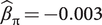 $ {\hat{\beta}}_{\pi }=-0.003 $
with
 $ \mid {\hat{t}}_{\pi}\mid =1.09 $
, so becomes insignificant. Table 3 records the correlation between
 $ {\Delta}_{12}U $
and
 $ \pi $
for the in-sample and forecast periods. The correlation is effectively zero over 2020. To disentangle this effect, we apply a subset of multiplicative indicator saturation (MIS; see Castle et al., Reference Castle, Hendry and Martinez2017) to identify parameter nonconstancy in the model. We include
 $ {\pi}_t\times {S}_{2020(j)} $
for
 $ j=1,\dots, 9 $
, where
 $ {S}_{2020(j)} $
is a step indicator that takes the value 1 for observations 2020(1)–2020(
 $ j $
) [2020(9) is the end of the sample], in model (2). All regressors in the model are fixed apart from the interaction terms, and we select at
 $ \alpha =0.001 $
using Autometrics.
 $ {\pi}_t\times {S}_{2020(3)} $
is retained leaving the full sample
 $ {\pi}_t $
coefficient close to that from (2) using data to 2019(12). The method successfully detects the induced shift in our estimated model following the policy intervention which began in March, and reveals that the apparent change in the coefficient of
 $ \pi $
is due to the shift in policy.
Correlation between
 $ \pi $
and
 $ {\Delta}_{12}U $

Forecast failure is often due to structural breaks in the data that are not captured by the economic model. Here, the model predicts a structural break in the data which does not materialise. This is because policy intervention changes the earlier constant relationships captured in the economic model by artificially holding down measured unemployment rates via the furlough scheme and other economic policies. We view these conditional forecasts from the economic model as scenario forecasts answering the question ‘what would the unemployment rate have been if the policy intervention had not occurred?’
4.2.2. Forecasting with a policy intervention dummy
MIS revealed a significant indicator in March which we use to capture the effect of the UK’s Covid-19 policies. Over the forecast period, the UK underwent its first national lockdown, with accompanying economic policies. Lockdown restrictions requiring nonessential businesses to close were imposed on 23 March 2020, and the UK announced a job retention scheme, aimed to support employers who could not maintain the current workforce, because their operations were affected by coronavirus. The scheme, also known as the furlough scheme, paid 80 per cent of workers’ salaries. The aim of the furlough policy was to mitigate the impact of lockdown on recorded unemployment, so will have a direct effect on our forecasting model. We take the econometric model (2), fixing the in-sample parameters, and add a ‘lockdown’ dummy given by
 $$ {\displaystyle \begin{array}{l}{D}_f=1\hskip0.72em \mathrm{for}\ \mathrm{March},\mathrm{April},\mathrm{May};\\ {}{D}_f=0\hskip0.82em \mathrm{otherwise}.\end{array}} $$
Alternative taperings could be considered, as the economic impact will be due to changing behaviour as well as government policy. However, behavioural changes are harder to measure, and so linking dummies to explicit policies holds appeal. This also means that the model can be tested over the second and third national UK lockdowns when the unemployment data become available.
Although lockdown was only introduced on 23 March, the evidence from MIS suggests that there is a sufficient shift in March to commence forecasting in April using data up to March. Estimates of the lockdown dummy are given in table 4. The dummy is poorly estimated on March data alone, so there is not enough information to improve the forecast for April. However, estimating the model up to April leads to a highly significant lockdown dummy which heavily adjusts the forecasts of unemployment. By May, there are stable estimates of the policy intervention dummy, dampening the forecasts from the model without policy intervention.
Parameter estimates for the lockdown dummy included in (2)

The forecasts for 1–3-month ahead are recorded in figure 11 [panel (b)]. The first three sets of forecasts are identical to those in panel (a). The next set of forecasts made in March show a small reduction in forecast error relative to the unadjusted model (an average forecast error over
 $ h=\mathrm{1,2,3} $
of 1 per cent compared to a forecast error of 1.26 per cent for the unadjusted model). With just one more observation to estimate the lockdown dummy, the improvement in forecast accuracy is substantial (averaging over the three forecast horizons, the forecasts made in April have an average forecast error of 0.18 per cent relative to 0.67 per cent for the unadjusted model). The forecasts are the same after the lockdown dummy ends, but during lockdown, the adjustment significantly improves the forecast performance of the econometric model.
To get a sense of the magnitude of the forecast differences, in the 3-month period from April to June 2020, there were 1.338-million people unemployed in the UK. In April, the econometric model predicted there would be 1.546-million people unemployed for the same period.Footnote 7 The same model including the lockdown dummy predicted 1.377-million unemployed, a difference of 169,000 people. Interpreting this difference as a scenario, whereby the level of unemployment would have been 169,000 higher had furlough and other related policies not been implemented, suggests that the economic response was fundamental to holding unemployment down in the first wave of the pandemic.
4.3. Unconditional econometric forecasts
The forecasting model (2) conditions on contemporaneous data,
 $ {\pi}_t $
, and hence a comparison with unconditional forecasts will be based on different information sets. To make the econometric model forecasts unconditional, we replace the known
 $ {\pi}_{T+h} $
, where
 $ T $
is the forecast origin and
 $ h $
is the forecast horizon, with forecasts of
 $ {\hat{\pi}}_{T+h\mid T} $
using Cardt to forecast the profits proxy. Castle et al. (Reference Castle, Doornik and Hendry2018) examine when contemporaneous regressors should be retained in forecasting models if they also need to be forecast, given that structural breaks occur in the conditioning variables. Despite conditioning on a subset of the information set available for the conditional econometric model forecasts, table 5 shows that the unconditional forecasts are more accurate over March and April when the pandemic took hold. The extrapolative Cardt forecasts of
 $ {\pi}_t $
were poor in March and April when profits fell dramatically.
 $ {\hat{\pi}}_t $
missed the fall initially, but these poor forecasts helped the econometric model to avoid predicting a large rise in the unemployment rate. The forecast error in the profits proxy is a measure of the economic policies implemented in March and April. However, moving forward to May and June, forecasts of the profits proxy miss the rebound, predicting very large negative values. This impacts on the econometric model forecasts, leading the unconditional forecasts to perform much worse. The comparison of conditional and unconditional forecasts show that more information does not always lead to improved forecast performance as structural breaks impact on the forecasts in different ways.
Absolute forecast errors (
 $ \times 100 $
) for unemployment forecasts over 2020. Unconditional econometric are unconditional forecasts from the econometric model using Cardt to forecast the contemporaneous profits proxy
 $ {\pi}_t $
. Average is the equally weighted average of the conditional econometric and Cardt forecasts. Bold indicates smallest absolute forecast errors

Abbreviations: MAPE, mean absolute percentage error; MPE, mean percentage error.
4.4. Forecasting the unemployment rate using Cardt
The econometric model forecasts can be used as a counterfactual to measure what effect the pandemic would have had on unemployment if the economic policies that accompanied the first lockdown had not been implemented. We can think of the econometric model as describing ‘business as usual’ as the model specification and estimation is fixed prior to the pandemic, thus reflecting the predicted unemployment rate had no mitigation policies, including furlough, been implemented. To contrast, we use the extrapolative statistical forecasting device, Cardt, to forecast unemployment. This device does not account for any specific economic and policy measures implemented over the forecast horizon but relies on extrapolating recent trends in the data. The method worked well for the Covid-19 data, so it is of interest whether it also produces reasonable forecasts for the unemployment rate. The forecasts are recorded in figure 11 [panel (c)]. The statistical forecasts are much closer to the outturns until June when the unemployment rate starts to rise, but the extrapolative forecasts do not. In April, Cardt predicted 1.321-million unemployment in the three months from April to June 2020, which is a difference of 225,000 people compared to the ‘business as usual’ econometric model.
Cardt also provides a useful benchmark against published forecasts. The Bank of England (BoE) unemployment rate forecasts from the Monetary Policy Report in January 2020Footnote 8 predict an unemployment rate of 3.8 per cent for 2020Q1, very close to our Cardt forecasts. In the May Monetary Policy Report,Footnote 9 the BoE offer a scenario with the unemployment rate rising to almost 10 per cent before falling back in 2021, and by August,Footnote 10 they predict a rate of 7.5 per cent in 2020Q4. Cardt predicts an unemployment rate of 4.7 per cent for 2020Q4 based on data available to August 2020, substantially lower than the forecast produced by the BoE, and a difference of 960,000 people (assuming a constant economically active population at September 2020 levels). Being data-based, Cardt forecasts are influenced by the furlough having reduced measured unemployment.
4.5. Forecast comparisons
Table 5 records the absolute forecast errors for the conditional econometric model with contemporaneous
 $ {\pi}_t $
, the unconditional econometric model with forecast
 $ {\hat{\pi}}_t $
, the conditional model with the lockdown policy dummy and the statistical forecasts. The row ‘Average’ reports the equally weighted forecasts from the conditional econometric model and Cardt, with the forecasts recorded in figure 11 [panel (d)]. MAPE denotes the mean absolute percentage error for a given horizon across all months in the forecast period, and MPE denotes the mean percentage error.
The statistical model produces some of the most accurate forecasts up to and including May for all horizons, with substantial reductions in forecast errors relative to the conditional econometric model throughout the lockdown period. The econometric model forecasts are poor in April and May when policies such as furlough played a significant role, and could be seen as the counterfactual unemployment rate had such a policy not been introduced. Accounting for the policy takes some time, but it can improve the econometric model forecasts, as seen for the two months when the policy dummy can be accurately estimated. For 3-month ahead, the lockdown policy dummy has no effect throughout April and May because of the 3-month lead time, but it does improve the forecasts for June and July. The average is never the best forecast (except for the 3-month ahead forecast in July), but both minimizes the risk of very large forecast errors and has the smallest MPE. The unconditional econometric forecasts are the best more than 40 per cent of the time, but also occasionally the worst.
Ericsson (Reference Ericsson1992) proposes a forecast encompassing test that assesses the ability of one set of forecasts to explain the errors of another forecasting device allowing for the forecasts to be cointegrated. This builds on the encompassing principle developed by Mizon and Richard (Reference Mizon and Richard1986) and the test of forecast encompassing by Chong and Hendry (Reference Chong and Hendry1986; see also Hendry, Reference Hendry1988). Let
 $ {\hat{y}}_{t\mid t-j} $
and
 $ {\tilde{y}}_{t\mid t-j} $
denote two sets of forecasts from the models in table 5, with
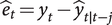 $ {\hat{e}}_t={y}_t-{\hat{y}}_{t\mid t-j} $
and
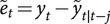 $ {\tilde{e}}_t={y}_t-{\tilde{y}}_{t\mid t-j} $
as the forecast errors, where
 $ j=\mathrm{1,2,3} $
, and
 $ t=2020(1)-2020(9) $
. The forecast encompassing tests for both directions are given by
 $$ {\displaystyle \begin{array}{l}{\hat{e}}_t={\lambda}_0+{\lambda}_1\left({\tilde{y}}_{t\mid t-j}-{\hat{y}}_{t\mid t-j}\right)+{\eta}_{1,t},\\ {}{\tilde{e}}_t={\delta}_0+{\delta}_1\left({\hat{y}}_{t\mid t-j}-{\tilde{y}}_{t\mid t-j}\right)+{\eta}_{2,t}.\end{array}} $$
If
 $ {\mathrm{H}}_0:{\lambda}_1=0 $
is rejected, the difference between
 $ {\tilde{y}}_{t\mid t-j} $
and
 $ {\hat{y}}_{t\mid t-j} $
helps to explain the forecast errors from model
 $ \hat{\cdot} $
, and hence
 $ {\tilde{y}}_{t\mid t-j} $
provides information above and beyond what is available from the
 $ {\hat{y}}_{t\mid t-j} $
forecast. Likewise, if
 $ {\mathrm{H}}_0:{\delta}_1=0 $
is rejected, we conclude that
 $ {\hat{y}}_{t\mid t-j} $
forecast encompasses
 $ {\tilde{y}}_{t\mid t-j} $
.
The encompassing test is normally distributed as
 $ T,H\to \infty $
, but our sample size is very small. Hendry (Reference Hendry1986) provides power functions of the Chong and Hendry (Reference Chong and Hendry1986) encompassing test for
 $ H=5,\dots, 14 $
, for the case when both forecasting models are misspecified and finds a fair degree of power. Gaussianity of the disturbances in (5) is required for small sample analysis using the t-distribution, but that assumption does not hold for our forecasts. As a check, we conduct a simulation study to evaluate the power of the encompassing test, reported in table 6.Footnote
11 For the forecast encompassing case where a second forecasting model provides no additional information over and above the forecasts from the first model, the power to detect forecast encompassing declines substantially for small samples. When neither model forecast encompasses the other as both forecasts yield additional information, the power is still quite high even in very small samples, and does not fall by much under non-normal errors. These results are close to the power estimates in table 3 of Hendry (Reference Hendry1986). Therefore, we proceed with the empirical encompassing tests, but note that the power may be low given the small sample.
Probability of rejection of the null hypothesis for the Ericsson (Reference Ericsson1992) encompassing test

Table 7 records the results from the forecast encompassing tests. For each row, forecasts from model M1 are denoted
 $ {\hat{y}}_{t\mid t-j} $
in (5) and forecasts from model M2 are denoted
 $ {\tilde{y}}_{t\mid t-j} $
. In the first row, there is evidence that the unconditional model forecasts provide information above that contained in the conditional model forecasts. This is striking as the unconditional forecasts use a reduced information set with forecasts of the profits proxy. There is no strong evidence that the conditional model forecasts encompass the unconditional model forecasts, so they do not capture additional information relative to the unconditional forecasts. The following three rows test various specifications of the econometric model against the statistical forecasts. There is statistically significant evidence that Cardt forecast encompasses the econometric model at all forecast horizons. Hence, there is a clear benefit to using statistical forecasts during periods subject to structural breaks.
Forecast encompassing tests statistics for 2020 unemployment rate forecasts. Coefficient estimates from (5) are reported with estimated standard errors in parentheses and estimated t(
 $ df $
)-statistics in square brackets.
 $ df=7 $
for 1 month,
 $ df=6 $
for 2 months and
 $ df=5 $
for 3 months.
 $ {}^{\ast } $
,
 $ {}^{\ast \ast } $
and
 $ {}^{\ast \ast \ast } $
denote significance at 10 per cent, 5 per cent and 1 per cent, respectively

As a benchmark comparison, we consider the same forecasts over 2019, recorded in figure 13 with table 8 reporting the forecast errors and table 9 reporting the forecast encompassing test statistics. All forecasts are more accurate given the stable environment, but the conditional econometric model forecasts produce the smallest forecast errors on average. The unconditional forecast errors are close to those of the conditional forecast errors, so the costs of forecasting contemporaneous regressors using Cardt are small, and negative in some cases where the unconditional forecasts deliver the smallest forecast errors of all models considered. At the 2- and 3-month horizons, there is evidence that both the conditional and unconditional forecasts encompass each other, so both yield additional information. This implies the Cardt forecasts of the profits proxy do contribute additional information. The forecast errors from Cardt are mostly larger than those for the econometric model, although table 9 shows that they also forecast encompass the econometric model. There is additional information in both the econometric model forecasts and the statistical forecasts, with significant forecast encompassing tests in both directions. As all forecast errors are in the same direction, averaging does not help.
(Colour online) Panel (a): conditional 1–3-month ahead forecasts from the econometric model over 2019. Panel (b): unconditional 1–3-month ahead forecasts using Cardt over 2019

Absolute forecast errors (
 $ \times 100 $
) for unemployment forecasts over 2019. Unconditional are unconditional forecasts from the econometric model using Cardt to forecast the contemporaneous profits proxy
 $ {\pi}_t $
. Average is the equally weighted average of the conditional econometric and Cardt forecasts. Bold indicates smallest forecast errors

Abbreviations: MAPE, mean absolute percentage error; MPE, mean percentage error.
Forecast encompassing tests statistics for 2019 unemployment rate forecasts. Coefficient estimates from (5) are reported with estimated standard errors in parentheses and estimated t(
 $ df $
)-statistics in square brackets.
 $ df=10 $
for 1 month,
 $ df=9 $
for 2 months and
 $ df=8 $
for 3 months.
 $ {}^{\ast } $
,
 $ {}^{\ast \ast } $
and
 $ {}^{\ast \ast \ast } $
denote significance at 10 per cent, 5 per cent and 1 per cent, respectively

The switch in rankings from 2019 to 2020, and the shift to unidirectional forecast encompassing for Cardt, highlights the value of different forecasting methodologies at different points in the forecast period due to the impact of structural breaks and policy interventions. The substantial and significant forecast improvements using Cardt over the lockdown period mean that over the forecast sample, this statistical forecasting method performs best overall, but in quiescent periods, a model embodying our theoretical understanding of the economy yields advantages. If the most appropriate forecasting model is not known, pooling using an equally weighted average can reduce large forecast errors if the forecasting models are differentially biased.
5. Conclusions
Forecasting has come under the spotlight during the Covid-19 pandemic, with a huge number of publicly available forecasts for cases and deaths. The economic impact of the pandemic also needs to be forecast, facing large variations in policy and economic responses across the world. In a simplified characterisation of forecasting methodology, we categorise forecasts into two broad classes; those based on epidemiological or structural theory-based models, and those based on statistical extrapolations. In this paper, we argue that the very nature of the pandemic means that wide-sense nonstationarity, particularly in the form of structural breaks, is present in the data. As such, forecasting models must be adaptive to these shocks. Structural models tend to have inbuilt equilibria and are therefore not rapidly adaptive, whereas statistical forecasting models can be designed to adapt rapidly to shocks by ensuring there are no equilibria in the forecasting model. We demonstrate the forecast performance of such a model in the context of both Covid-19 data and corresponding unemployment data. We also show how the statistical forecasts can be used to produce unconditional forecasts from conditional models, embedding forecasts of contemporaneous regressors in the forecasting model.
There are drawbacks of the Cardt methodology in that it cannot be used to assess policy implications or undertake scenario analysis. However, the unemployment forecasting example shows that comparing econometric model forecasts with extrapolative forecasts can be highly informative as to the effects of current policy, thereby providing a measure of the effect of policy on the outcome. Such large forecast errors for the econometric model relative to those of Cardt show the success of the UK furlough scheme in maintaining employment during lockdown, but forecasts for the summer months suggest that the policy delayed rather than mitigated the rise in unemployment. The pandemic has highlighted the need for both forms of forecast, with a portmanteau approach to forecasting more relevant in the pandemic era.
Acknowledgements
Financial support from the Robertson Foundation (award 9907422), the Institute for New Economic Thinking (grant 20029822), and the ERC (grant 694262, DisCont) is gratefully acknowledged. All calculations and graphs use OxMetrics (Doornik, Reference Doornik2018) and PcGive (Doornik and Hendry, Reference Doornik and Hendry2018). We thank participants of the NIESR workshop on the impact of Covid-19 Pandemic on Macroeconomic Forecasting, 20 November 2020, and the 40th International Symposium of Forecasting, 26 October 2020, and an anonymous referee for helpful comments.
Data appendix
Lower cases represent logs,
 $ \Delta {x}_t $
represents the monthly change in
 $ {x}_t $
and
 $ {\Delta}_{12}{x}_t $
represents the annual change in
 $ {x}_t $
. ∗https://www.ons.gov.uk/employmentandlabourmarket/peopleinwork/earningsandworkinghours/datasets/averageweeklyearningsearn01

Abbreviation: ILO, International Labour Organization; NSA, not seasonally adjusted.