


Individuals vary in how much they care about specific policy issues (e.g.,Hill, Reference Hill2022a; Cavaillé et al., Reference Cavaillé, Chen and Van der Straeten2025).Footnote 1 When they passionately support or oppose a particular policy, they can signal the intensity of their preferences through costly actions such as letter-writing campaigns, hiring lobbyists, making campaign contributions or public comments, and participating in mass protests. Both elected and appointed officeholders can and do adjust their choices in response to these forms of costly signals of preference intensity (e.g.,Fording, Reference Fording2001; Madestam et al., Reference Madestam, Shoag, Veuger and Yanagizawa-Drott2013; Kalla and Broockman, Reference Kalla and Broockman2016; Acemoglu et al., Reference Daron, Hassan and Tahoun2018).
Existing empirical studies of policy representation, however, often neglect preference intensity in their analysis. Canonical American politics scholarship on policy responsiveness and congruence uses dichotomous survey measures (e.g., favor or oppose, agree or disagree, approve or disapprove) to gauge public opinion on state policies and examines whether the majority opinion matches actual policy implementation status (e.g., Matsusaka, Reference Matsusaka2010; Lax and Phillips, Reference Lax and Phillips2012; Caughey and Warshaw, Reference Caughey and Warshaw2022). These studies estimate positive correlations between opinion and policy—indicating favorable responsiveness—but document a lack of congruence in the American states. Yet focusing exclusively on preference directionality without paying attention to preference intensity may miss out on important political dynamics and may help explain why scholars have documented relatively low levels of congruence. In reality, politicians can respond to “intense minorities” rather than a “less-intense majority” (Hill, Reference Hill2022b), something binary directional measures cannot capture. To better understand policy representation in the United States, it is important to take preference intensity into account.
Scholars have typically been unable to incorporate measures of preference intensity into their analyses of state policy responsiveness to public opinion due to the challenges of estimating variation in preference intensity in the mass public. Preference intensity is difficult to measure from survey reports because of respondents’ incentives to misreport the intensity of their beliefs (Krosnick et al., Reference Krosnick, Boninger, Chuang, Berent and Carnot1993; Miller and Peterson, Reference Miller and Peterson2004; Lenz, Reference Lenz2012).Footnote 2 Political scientists typically resort to Likert items, but an underlying problem is that respondents often exaggerate their views by self-reporting strong—yet often insincere—preferences (Cavaillé et al., Reference Cavaillé, Chen and Van der Straeten2019; Hanretty et al., Reference Chris, Lauderdale and Vivyan2020).
Given the importance of measuring preference intensity and the lack of quality survey instruments to measure it, scholars have developed Quadratic Voting for Survey Research (QVSR) (Casella, Reference Casella2005; Quarfoot et al., Reference Quarfoot, von Kohorn, Slavin, Sutherland, Goldstein and Konar2017; Cavaillé et al., Reference Cavaillé, Chen and Van der Straeten2019; Casella and Sanchez, Reference Casella and Sanchez2022). Drawing on insights from social choice theory (Goeree and Zhang, Reference Goeree and Zhang2017; Patty and Penn, Reference Patty and Penn2017; Lalley and Weyl, Reference Lalley and Weyl2018), this innovative method allows researchers to measure individual-level preference intensity by asking survey participants to use an endowment of virtual credits to buy votes for a predefined set of alternatives (e.g., policy proposals).Footnote 3 The number of votes individuals cast in favor of or against a particular alternative thus reveals their preference for that alternative, relative to other alternatives. Scholars have presented evidence that this approach measures preference intensity toward policy alternatives more accurately than conventional Likert items (Quarfoot et al., Reference Quarfoot, von Kohorn, Slavin, Sutherland, Goldstein and Konar2017; Cavaillé et al., Reference Cavaillé, Chen and Van der Straeten2019, Reference Cavaillé, Chen and Van der Straeten2025) and have applied it to study important policy questions such as mass preferences for public transit, bilingual education, teachers’ tenure, and immigration enforcement standards (Casella and Sanchez, Reference Casella and Sanchez2022; Holland, Reference Holland2023) as well as to test new theories about voter behavior (Kamphorst, Reference Kamphorst2024).
In this article, we leverage the recent advances in survey methodology and devise an original national survey ( $N=7,084$) to measure Americans’ preference intensity toward a diverse set of 10 state policies that have direct correspondence to state laws. The rich data allow us to operationalize policy preferences—not only directionality but also intensity—in multiple reasonable ways by using the Likert scale, the “most important policy” item, and QVSR. Because QVSR is still nascent in the social sciences, we also embed a novel experiment that allows us to evaluate its validity as a measurement approach, and our preregistered analysis substantiates its validity. After validation, we extract state-level preference intensity of each policy and analyze how strongly it predicts actual policy implementation in each American state.
We find that using measures that account for the intensity of policy support relative to the intensity of the opposition—including both traditional Likert and new QVSR measures—does not meaningfully improve the overall level of congruence between public opinion and public policy in the American states. Across 10 state policies ranging from affirmative action and school vouchers to the death penalty and gun laws, policies that prevail under state-wide quadratic voting are implemented in US states only around half the time—not meaningfully different from random chances. We thus contribute new evidence that the lack of policy representation in the American states remains—even if preference intensity is systematically integrated into the empirical analysis.
1. Policy representation in the American states: existing evidence
Whether policymaking reflects political preferences of the mass public is a central question in both American politics (e.g., Bartels, Reference Bartels2008; Bafumi and Herron, Reference Joseph and Herron2010; Canes-Wrone, Reference Canes-Wrone2015) and comparative politics (e.g., Giger and Klüver, Reference Giger and Klüver2016; Rasmussen and Reher, Reference Rasmussen and Reher2019; Lupu and Warner, Reference Lupu and Warner2022). This question is important because it concerns the health and functioning of democracy. Indeed, some political theorists consider policy representation an essential element of democracy (Pitkin, Reference Pitkin1967; Dahl, Reference Dahl1971).
In American politics, an early, influential treatment of the topic examines the mapping between voter ideology and aggregate policy outcomes. In their pioneering work, Erikson et al. (Reference Erikson, Wright and McIver1993) combine 12 years of national survey data and show that self-reported voter ideology strongly correlates with aggregate state policy. States with a higher proportion of self-reported conservative (or liberal) voters have a higher proportion of conservative (or liberal) policies in place. Drawing on similar methods, Erikson et al. (Reference Erikson, MacKuen and Stimson2002) reach the same conclusion at the national level. However, as Lax and Phillips (Reference Lax and Phillips2012, 148) note, “by focusing on the ideology-policy correlation, [this line of work] does not assess how responsive states are to voter preferences on specific policies. Nor does it tell us how effective state political systems are at translating opinion majorities into public policy.” The former critique taps into responsiveness, and the latter captures congruence—both of which are important facets of policy representation (Canes-Wrone, Reference Canes-Wrone2015). Another important limitation of this early literature is that self-reported ideology may not be an appropriate indicator of substantive policy preferences, as recent research shows (Jefferson, Reference Jefferson2024; Yeung and Quek, Reference Yeung and Quek2025; cf. Kollman and Jackson, Reference Ken and Jackson2026). Accurately characterizing state-level policy preferences requires more fine-grained measures.
A subsequent literature takes a more targeted approach to measure policy preferences. It draws on specific question items from existing national surveys that ask for respondents’ opinion on state policies. These studies focus on policy representation in salient sociocultural policy issues at the time, including abortion, the death penalty, and gay rights (Gerber, Reference Gerber1999; Lax and Phillips, Reference Lax and Phillips2009a). Because the surveys they rely on to measure policy preferences are typically “yes/no” or “favor/oppose” questions, this literature does not account for preference intensity in the empirical analysis. Using such dichotomous measures of policy preferences that capture preference directionality absent intensity, these studies find that American state policies were responsive to public opinion in the specific policies they examine Gerber (Reference Gerber1999), yet there is “a surprising amount of noncongruence” (Lax and Phillips, Reference Lax and Phillips2009a, 367).
Diversifying the set of state policies analyzed, subsequent work builds on this literature and finds that while American state policies are responsive to public opinion, they are congruent with majority will only roughly half the time. Using national surveys disaggregated to the state level to examine whether majority public opinion in a state is congruent with the state’s implemented policy on 10 high-profile issues, Matsusaka (Reference Matsusaka2010, 143) finds that majority public opinion and state policy are congruent in 59% of the cases and that the level of congruence is almost identical at 60% when accounting for preference intensity by limiting the sample to respondents with “strong” preferences.Footnote 4 Examining a broader set of policy issues and using multilevel regression with poststratification to estimate state-level policy attitudes (as opposed to direct measurement through disaggregating surveys to the state level), Lax and Phillips (Reference Lax and Phillips2012) find that 48% of the state-policy pairs in their analysis are congruent with majority public opinion. Both of these studies find similarly low levels of congruence despite using different methodological approaches and analyzing distinct sets of policy issues.
Instead of looking at congruence at a single point in time, Caughey and Warshaw (Reference Caughey and Warshaw2022) take a dynamic view of the relationship between public opinion and policymaking in the states. They find that over longer periods of time, there is more evidence of state policies and public opinion converging than in a single cross-section. When an issue first enters the agenda, “policy matches majority opinion only 40 percent of the time; three decades later, policy congruence averages 70 percent” (Caughey and Warshaw, Reference Caughey and Warshaw2022, 5). Their finding of low levels of baseline congruence illustrates that congruence is often quite low in the American states.
This important body of empirical work on policy representation has inspired a productive literature that examines the causes of poor representation in the United States, such as elite misperception (e.g., Broockman and Skovron, Reference Broockman and Skovron2018), economic inequality (e.g., Gilens, Reference Gilens2012), and political sophistication (e.g., Rogers, Reference Rogers2023). A major limitation of this body of scholarship, however, is its continued reliance on survey items that do not account for preference intensity. Thus, it remains unclear whether and how these empirical findings—relatively high responsiveness but low congruence—will change if we integrate the role of preference intensity into the empirical assessments. Hill’s (Reference Hill2022a, Reference Hill2022b) intensity theory clarifies why additionally taking preference intensity into account will generate new and important insights into the quality of US democracy in terms of policy representation. Formalizing the logic with game-theoretic models, he shows that a lack of policy congruence with majority will does not necessarily imply a lack of policy representation. When majorities in society hold generally weak preferences for policies in one direction whereas minorities hold relatively strong preferences in the opposite direction, policy outcomes congruent with the latter—which create “frustrated majorities” (Hill, Reference Hill2022b) or “democratic deficits” (Lax and Phillips, Reference Lax and Phillips2012)—can be indicative of high political accountability. To communicate their intensity to politicians, intense minorities are often willing to take costly political actions to signal their policy preferences (Hill, Reference Hill2022b, Chapters 9 and 10). Office-seeking politicians, aware of such costly signals and responsive to public opinion, may in turn adopt policies in favor of more-intense minorities—instead of less-intense majorities.
Hence, while existing scholarship has demonstrated the lack of congruence of US state policies with majority will, intensity theory implies that such non-majoritarian outcomes may not reflect a lack of policy representation in American politics (Hill, Reference Hill2022b). What would look like low congruence from one perspective (i.e., policy passed despite majority opposition) might be evidence of high congruence from another (i.e., policy passed because the minority in favor cared more than the majority against). Thus, measuring congruence in ways that overlook preference intensity—as well as the role of preference intensity in representative democracy—will return more pessimistic conclusions than warranted regarding policy representation in the United States. Theoretically, it is possible that state policies map well onto citizen preferences at the state level if we factor in the role of preference intensity in shaping politicians’ choices.
Importantly, this possibility can be empirically evaluated if we have reliable measures of preference intensity. Yet because existing opinion surveys cannot reliably elicit preference intensity of state policies, the literature remains unclear about whether and how estimated policy representation in the United States changes if we explicitly integrate preference intensity into the empirical analysis.Footnote 5 We take on this empirical challenge by developing and implementing an original national survey to measure public opinion that incorporates preference intensity in multiple ways, followed by mapping state-level policy preferences onto actual policy outcomes in the United States to reassess its policy representation.
2. Data and methods
We fielded a large-scale survey on a sample of 7,084 American adults via Lucid in September and October 2022. Our sample, albeit not nationally representative, closely mirrors several key demographics in the United States, including age, sex, and state of residence (Supplementary Appendix A). To address data quality concerns (Ternovski and Orr, Reference Ternovski and Orr2022), we show in Supplementary Appendix I that respondents spent nontrivial time on our quadratic voting task and that policy attitudes reflected in our survey reasonably mirror those reflected in existing representative surveys. We further show that self-reported policy preferences by Democrats and Republicans diverge in expected ways in Supplementary Appendix I, suggesting that our preference intensity measures capture meaningful variations in respondents’ policy preferences rather than random noise.
2.1 Survey design
We began the survey with a mix of standard demographic questions and attention checks. We then randomized the sequence by which respondents expressed their policy preferences through the Likert module or the QVSR module. In Supplementary Appendix E, we show that there is no order effect on our QVSR measures of policy preferences. In both modules, we randomized the choice set by using complete randomization to present 5 of 10 policies to each respondent:
1. A law requiring abortions to be performed by licensed physicians
2. Affirmative action admissions programs at colleges and law schools that give racial preferences to minority applicants
3. Allowing students to receive vouchers to pay tuition and attend private schools
4. A law requiring voters to show an official photo identification on Election Day to cast a vote
5. Term limits on state legislatures
6. A law protecting gays and lesbians from prejudice and discrimination in housing
7. Issuing driver’s licenses to unauthorized immigrants
8. A law requiring criminal background checks for all handgun sales
9. Death penalty for a person convicted of murder
10. Legalization of marijuana for nonmedical use
After respondents completed both modules, we asked them which of the five policies they saw was most important to them. We explicitly stated that their choice could be a policy that they felt most important to favor or oppose. They could only pick one policy proposal.
We note the variety of these policies. First, they are diverse in terms of issue areas—ranging from abortion to education, from gay rights to gun rights, and from election law to marijuana law. Such issue diversity allows us to examine policy representation holistically and avoid drawing conclusions about responsiveness and congruence based on single issues, consistent with existing contributions such as Caughey and Warshaw (Reference Caughey and Warshaw2022) and Lax and Phillips (Reference Lax and Phillips2012). Second, the policies we included are diverse in terms of policy salience. Policy debates over voter ID and firearm regulations are much more prevalent than those over term limits for state legislators, for example, in contemporary US politics. There is also strong evidence of variations in policy salience in our data based on our “most important policy” measure (Table 1). Such diversity in salience is important because past research has identified salience as a determinant of policy responsiveness (Lax and Phillips, Reference Lax and Phillips2009a).
Policy salience as indicated by self-reported most important policy

Table 1 Long description
Percentages report how often each of 10 policies was selected as the single most important policy, with 95% confidence intervals shown for each estimate. Gun law stands out as the top choice at 41.04% (about 39.41% to 42.69%). A second tier includes photo ID for voting at 24.54% (23.12% to 26.00%), nonmedical marijuana at 22.42% (21.06% to 23.84%), MD-only abortion at 20.22% (18.92% to 21.59%), and term limits at 19.33% (18.05% to 20.68%). Gay housing law is 18.01% (16.77% to 19.32%) and school vouchers 16.35% (15.15% to 17.62%). Lower-salience items include the death penalty at 14.75% (13.60% to 15.97%), immigrant rights at 12.25% (11.20% to 13.39%), and affirmative action at 11.21% (10.19% to 12.31%). An exploratory chi-squared test indicates the proportions are not equal across policies, so differences in salience are unlikely to be due to random variation alone.
Notes: 95% confidence intervals are shown in brackets. The last row reports the result from an exploratory chi-squared test on the equality of proportions of percentage of “most important” responses across the 10 policies.
To maximize comparability between results from the Likert, QVSR, and “most important policy” modules, we assigned the same policy bundle to each respondent across all modules. For the Likert module, we asked respondents to express their views on the five policies that we randomly assigned to them. Their options took a standard 5-point Likert scale, ranging from “strongly oppose” to “strongly favor.” For the QVSR module, because we asked our respondents to vote on five policies, we allocated a budget of 25 virtual voting credits to them in the spirit of quadratic voting (Lalley and Weyl, Reference Lalley and Weyl2018). We provided respondents with detailed but easy-to-understand instructions to explain how they could use the 25 virtual voting credits to vote. Figure 1 shows our survey interface, programmed on Qualtrics, for the QVSR module.
Quadratic voting platform.

Figure 1 Long description
The table has two columns: Number of Votes Cast on a Policy Proposal and Cost in Credits. Row 1: 0 votes, 0 credits. Row 2: 1 vote, 1 credit. Row 3: 2 votes, 4 credits. Row 4: 3 votes, 9 credits. Row 5: 4 votes, 16 credits. Row 6: 5 votes, 25 credits. Below the table, instructions explain how to use 25 voting credits to favor or oppose policy proposals. Examples illustrate spending credits to favor or oppose policies, with a reminder that total credits spent cannot exceed 25. Voting options, in this particular example, include affirmative action programs, death penalty for convicted persons, law requiring criminal background checks for handgun sales, law requiring a license to buy a gun and issuing driver′s licenses to undocumented immigrants. Each policy has boxes for opposing or favoring, with a total box at the bottom.
Based on the QVSR and Likert measures, we document the distributions of policy preferences in Figure 2.
Distributions of policy preferences, QVSR versus Likert measures.

Figure 2 Long description
Twenty histograms comparing policy preferences for ten policies using votes and Likert scales. Each policy has two histograms: one for votes and one for Likert responses. The horizontal axis for votes ranges from negative 6 to 6 and for Likert scales from 1 to 5. The vertical axis for both is the number of respondents, ranging from 0 to 2000. A dashed vertical line represents the neutral point or mean. Policy 1: MD-Only Abortion shows a vote distribution centered around 0 with a peak at approximately 1500 respondents. The Likert scale peaks at 5 with around 1800 respondents, indicating strong support. Policy 2: Affirmative Action has a similar vote distribution with a peak near 0. The Likert scale also peaks at 5, showing strong support. Policy 3: School Voucher displays a vote distribution centered near 0, with the Likert scale peaking at 5, indicating support. Policy 4: Photo ID for Voting shows a vote distribution with a peak near 0 and a Likert peak at 5, suggesting strong support. Policy 5: Term Limit has a vote distribution centered around 0, with the Likert scale peaking at 5, indicating support. Policy 6: Gay Housing Law shows a vote distribution centered near 0, with the Likert scale peaking at 5, indicating support. Policy 7: Immigrant Rights displays a vote distribution centered around 0, with the Likert scale peaking at 5, indicating support. Policy 8: Gun Law shows a vote distribution with a peak near 0 and a Likert peak at 5, suggesting strong support. Policy 9: Death Penalty has a vote distribution centered around 0, with the Likert scale peaking at 5, indicating support. Policy 10: Marijuana shows a vote distribution with a peak near 0 and a Likert peak at 5, suggesting strong support. Overall, the histograms reveal that most policies have a central vote distribution with Likert responses skewed towards strong support, as indicated by peaks at 5. The dashed line consistently marks the neutral or mean point across all graphs.
2.2. Measuring preference intensity: a quadratic voting approach
One major methodological innovation of this article is the use of QVSR to provide new measures of preference intensity for state policy issues. Quadratic voting is a method of incorporating preference intensity into collective decision-making (Lalley and Weyl, Reference Lalley and Weyl2018).Footnote 6 Standard one person one vote approaches do not accommodate heterogeneity in the intensity of preferences across individuals, but there are contexts in which a minority has intense preferences in favor of a policy and a majority has weak preferences against a policy, and vice versa (Hill, Reference Hill2022b). Quadratic voting is one method for accounting for such heterogeneity by permitting the costly expression of preference intensity.Footnote 7 It allows individuals to cast more than one vote on a policy issue but the marginal cost of each vote is increasing. In its canonical form, the cost in credits is given by the square of the number of votes cast. Thus, casting one vote for or against a policy costs one credit, two votes cost four credits, three votes cost nine credits, etc. In a collective decision-making context over a binary policy, the policy will be implemented if it receives more than half of votes cast.
In a survey research setting, quadratic voting can be used to measure respondents’ preference intensity. Respondents are endowed with a fixed (and equal across respondents) budget of credits that they can use to express support for or opposition to a particular policy issue. If a respondent has intense preferences on policy issue A but weak preferences on policy issue B, then they can allocate more credits toward policy issue A.
QVSR requires respondents to trade off the relative importance of distinct policy issues. Unlike in an unconstrained survey where a respondent can choose the most extreme options on all policy issues, in QVSR, an individual cannot express maximally strong preferences on all policy issues because this would exceed the credit endowment. As Cavaillé et al. (Reference Cavaillé, Chen and Van der Straeten2019) demonstrate, the optimal number of credits used on a particular policy area will depend on the relative importance of that policy issue compared to all of the other policy issues included in the survey. This naturally raises questions about how estimates of preference intensity would vary depending upon the issues that are included in the bundle of policy questions. A respondent who is asked to express their opinions on five issues that they have intense preferences over will allocate their voting credits more uniformly than an otherwise identical respondent who is asked to express their opinion on one issue that they have intense preferences over and four trivial issues.
To address this methodological concern, we take an experimental approach. Because we randomly assigned the policy bundles in our survey, we can experimentally test whether preference intensity, as measured by QVSR, is sensitive to the selection of the choice set. We evaluate the sensitivity of QVSR measures of preference intensity by following our preanalysis plan (https://osf.io/z23xu). We report the results in—and we refer interested readers to—Supplementary Appendix B, where we use preregistered analytical procedures to experimentally demonstrate the robustness of QVSR, a novel methodological contribution to the survey research literature.
2.3. Estimating state-level policy preferences
Given the stability of QVSR we demonstrated in Supplementary Appendix B, we extract state-level preference intensity of each policy from our rich survey data. Following the literature on state politics, we use multilevel modeling and poststratification (MRP) to estimate policy preferences at the state level (e.g.,Lax and Phillips, Reference Lax and Phillips2012; Caughey and Warshaw, Reference Caughey and Warshaw2022). Because we have around 3,500 individual survey responses for each policy, our sample is sufficiently large to apply MRP.Footnote 8 Although we do not have a nationally representative sample, MRP allows us to correct for differences between our sample and national benchmarks for a set of key variables, including age, sex, race, education, and region of residence. While reliable estimates of state-level public opinion are difficult to obtain for small states under a conventional disaggregation approach, MRP overcomes this challenge by leveraging demographic and geographic correlations in other states to compensate for small within-state samples. Because we have information about respondents’ state of residence and the characteristics of all states (e.g., region, population), poststratification allows us to account for between-state differences when estimating state-level public opinion. Therefore, while our state-level estimates of preference intensity are admittedly imperfect (as they come from an opt-in Internet sample), they are generally accurate given the strengths of MRP (Wang et al., Reference Wang, Rothschild, Goel and Gelman2015; Downes et al., Reference Marnie, Gurrin, English, Pirkis, Currier, Spittal and Carlin2018; Kennedy and Gelman, Reference Kennedy and Gelman2021).Footnote 9
Building on previous scholarship (e.g., Gelman and Hill, Reference Gelman and Hill2007; Lax and Phillips, Reference Lax and Phillips2009b), we estimate the following response model:
 \begin{equation}
\text{Number of Votes for Policy }k_{i} = \beta^0 + \alpha_{s[i]}^{state} + \alpha_{a[i]}^{age} + \alpha_{e[i]}^{edu} + \alpha_{g[i],r[i]}^{gender,race} + \varepsilon_{i},
\end{equation}
where individual-level random effects are modeled by  $\alpha_{a}^{age} \sim N\left(0,\sigma^{age}\right)$ for
 $a=1,\dots,6$,
 $\alpha_{e}^{edu} \sim N\left(0,\sigma^{edu}\right)$ for
 $e=1,\dots,5$, and
 $\alpha_{g,r}^{gender,race} \sim N\left(0,\sigma^{gender,race}\right)$ for
 $g=1,2$ and
 $r=1,\dots,4$.Footnote 10 Here, the outcome variable is the number of votes respondent
 $i$ casts in favor of Policy
 $k$ (
 $k \in \{1, \dots, 10\}$) in QVSR. It ranges from
 $-$5 to 5, with negative numbers indicating votes against the policy and positive numbers indicating votes in favor. This measure captures both preference directionality and preference intensity, outperforms other conventional measures of public opinion in predicting actual political behavior (Cavaillé et al., Reference Cavaillé, Chen and Van der Straeten2025), and, as our experiment showed, is generally insensitive to different policy bundles covered in our survey (Supplementary Appendix B).
State-level random effects, on the other hand, are modeled by
 \begin{equation}
\alpha_{s}^{state} \sim N\big(\gamma^{0}+\gamma^{south}\cdot south_{s}+\gamma^{northeast}\cdot northeast_{s}+\gamma^{west}\cdot west_{s}+\gamma^{repvote}\cdot repvote_{s},\sigma^{state}\big),
\end{equation}
where  $repvote_{s}$ is Donald Trump’s vote share in the 2020 presidential election in each state (
 $s=1,\dots,50$). While
 $i$ indicates an individual respondent,
 $s$,
 $a$,
 $e$,
 $g$, and
 $r$ index state, age category, education category, gender, and race category, respectively.
After using multilevel regression to model individual survey responses as a function of demographic and geographic typology, we poststratify by using the 2022 American Community Survey 5-Year data to weight the percentages of each demographic-geographic type with respect to actual state populations.Footnote 11 Because we have 50 states and 240 demographic types in each state, we obtain 12,000 combinations of demographic and state values, ranging from “White,” “Male,” “Age 18–29,” “No high school degree” in Alabama to “Hispanic,” “Female,” “Age 70+,” “Postgraduate degree” in Wyoming. Each combination  $c$ then corresponds to population frequency
 $N_c$ based on Census data. We then weight the prediction in each combination,
 $\theta_c$ (i.e., the predicted policy support given the relevant predictors and their estimated coefficients based on equation 1), by
 $N_c$. The average number of votes for each policy in each state is thus
 \begin{equation}
\text{Number of Votes for Policy }k^{\text{MRP}}_{s} = \frac{\sum_{c\in s}N_{c}\theta_{c}}{\sum_{c\in s}N_{c}}.
\end{equation}
If  $\text{Number of Votes for Policy }k^{\text{MRP}}_{s} \gt 0$, then the policy receives relative support in the state after accounting for preference intensity. We follow the same procedure to estimate state-level policy preferences based on other measures of individual policy attitudes:
• QVSR
 $^{-}$: a 3-point scale such that 1 indicates the respondent casts at least one vote in favor of the policy,
$-$1 the respondent casts at least one vote against the policy, and 0 the respondent does not cast any votes on the policy.
• Likert: a standard 5-point scale ranging from
$-$2 (strongly oppose) to 2 (strongly favor), with 0 indicating “neither favor nor oppose.” Compared to QVSR, this measure captures preference intensity with more noise and less precision, as recent research indicates (Quarfoot et al., Reference Quarfoot, von Kohorn, Slavin, Sutherland, Goldstein and Konar2017; Cavaillé et al., Reference Cavaillé, Chen and Van der Straeten2025).• Likert+: a 3-point scale such that 1 indicates the respondent favors the policy and rates the policy as most important to her,
$-$1 the respondent opposes the policy and rates the policy as most important, and 0 the respondent is neutral or does not rate the policy as the most important one. This measure leverages the “most important policy” question also available in our survey to operationalize preference intensity.• Likert
$^{-}$: a 3-point scale with 1 indicating “strongly favor” or “somewhat favor,”
$-$1 “strongly oppose” or “somewhat oppose,” and 0 “neither favor nor oppose.” This measure captures only preference directionality but not preference intensity, mirroring how canonical contributions in the policy representation literature estimate responsiveness and congruence in US states.Footnote 12


Figures S11–S15 in Supplementary Appendix F show our state-level estimates of policy preferences using each of the five alternative measures. We also report the correlations between the different measures of individual policy preferences in Table 2. In general, while all correlations are predictably positive, there are meaningful differences between QVSR-based measures and Likert-based measures. It follows that our analysis will be more comprehensive and robust if the estimates, based on different operationalizations of policy preferences, corroborate with each other and converge on the same conclusion.
Correlations between different measures of individual policy preferences

Table 2 Long description
Pairwise Pearson correlations compare four measures of individual policy preferences: QVSR, QVSR minus, Likert, Likert plus, and Likert minus. The highest correlation is between Likert and Likert minus at about 0.95, indicating very similar rankings across those two measures. QVSR and QVSR minus are also strongly related at about 0.88. QVSR has moderate correlations with Likert measures, around 0.52 with Likert, about 0.40 with Likert plus, and about 0.50 with Likert minus. QVSR minus correlates about 0.53 with Likert and Likert minus, but is weaker with Likert plus at about 0.30. Likert plus is moderately related to Likert at about 0.47 and to Likert minus at about 0.43. Standard errors are small throughout, suggesting these correlation estimates are precise, but correlations describe association rather than causation.
Notes: Entries are Pearson’s correlation coefficients. Standard errors are reported in parentheses.
Before proceeding to our analysis of policy representation, we hope to be transparent about the empirical assumptions underlying our QVSR-based measures.Footnote 13 One potential concern about the validity of QVSR as a measure of preference intensity is strategic voting: if the respondent has very strong preferences about issue A but thinks there is already a one-sided majority on that issue, the respondent might allocate votes to a closely contested issue B where the respondent’s votes might be pivotal. Drawing on related validation studies (Quarfoot et al., Reference Quarfoot, von Kohorn, Slavin, Sutherland, Goldstein and Konar2017; Cavaillé et al., Reference Cavaillé, Chen and Van der Straeten2025), our application assumes negligible strategic voting. A second assumption is that there is interpersonal comparability of intensity, in aggregate, between respondents voting in favor of the policy and respondents voting against it. This assumption appears reasonable as we have little theoretical reason to believe that the same number of votes would systematically mean different things to people favoring the policy versus people opposed to the policy. This assumption applies to Likert-based measures too (e.g., respondents who “strongly favor” and “strongly oppose” the policy have comparable levels of preference intensity).
3. Policy representation in the American states: a reassessment
In this section, we draw on our rich survey data and innovative measures to empirically examine the extent to which state-level preference intensity predicts actual policy outcomes in the United States. If preference intensity matters substantively but existing studies—which typically rely on simplistic, dichotomous measures that fall short of capturing intensity—have missed out on such dynamics methodologically, then we should observe reasonable levels of policy congruence based on at least some of our new measures that incorporate preference intensity into the estimation of state-level policy preferences. As the existing literature shows, policy congruence—defined as the alignment of the position that a majority of citizens support and the implemented public policy of the relevant political jurisdiction (Canes-Wrone, Reference Canes-Wrone2015, 149)—is generally low, with state policies matching majority opinion only around half the time (Matsusaka, Reference Matsusaka2010; Lax and Phillips, Reference Lax and Phillips2012), unless the policy has been on the agenda for decades (Caughey and Warshaw, Reference Caughey and Warshaw2022).
3.1. Main analysis
We begin by using the QVSR measure to investigate whether and how public opinion that accounts for preference intensity predicts actual policy outcomes at the state level. To do so, we compile a unique dataset that merges our estimates of policy preferences with the actual implementation statuses of the 10 policies in each state (as of the date we administered our national survey to the American public, i.e., September 26, 2022). Such mapping is possible because the 10 policies presented in our survey have direct correspondence to actual state laws in the United States (Supplementary Appendix F). Indeed, when we designed our survey, not only did we prioritize the variety of issue areas, but we also looked up specific state laws to ensure that (1) our question wording is directly comparable to actual state policies and (2) the implementation status of each policy has meaningful variations between states.
Table 3 shows the relationship between actual state policy outcomes and state-level public opinion, which captures preference intensity in multiple reasonable ways. For each policy and public opinion measure, we predict a state’s adoption of the policy by using our estimates of state-level policy preferences. Based on these data points ( $n = 50$ for each policy and public opinion measure, given that there are 50 states), we fit a logit regression for each of 10 policies:
 $\mathrm{Pr}\ (\text{Policy Adoption}_s = 1) = \text{logit}^{-1}(\alpha + \beta \text{State Opinion}_s)$, where
 $\text{State Opinion}_s$ is the average level of support for the given policy in state
 $s$, operationalized by using different QVSR-based and Likert-based measures of preferences. The slope of the regression,
 $\beta$, thus measures policy responsiveness: the more positive the slope, the higher the responsiveness (Lax and Phillips, Reference Lax and Phillips2012; Canes-Wrone, Reference Canes-Wrone2015). Here, we follow Canes-Wrone (Reference Canes-Wrone2015, 149) in conceptualizing responsiveness as “requir[ing] that if mass opinion moves in a particular direction, government officials become more likely to enact the policy advocated by that opinion.”
Responsiveness and congruence across different measures of public opinion

Table 3 Long description
State-level responsiveness estimates (with standard errors) and congruence rates are reported for 10 policies using five opinion measures: QVSR, QVSR minus, Likert, Likert plus, and Likert minus. In the combined analysis across all policies, responsiveness is positive for every measure, ranging from 4.41 (QVSR) to 11.35 (Likert plus), and congruence is similar across measures at about 44.2 to 46.6 percent. Several policies show strong positive responsiveness across most measures, including immigrant rights (about 36 to 159, highest under Likert plus), gay housing law (about 9 to 48), death penalty (about 14 to 35), and photo ID for voting (about 6 to 19). Some policies show negative responsiveness under many measures, such as school vouchers (about minus 2 to minus 20) and affirmative action (about minus 2 to minus 24), and nonmedical marijuana is mixed, with negative values for QVSR and Likert plus but positive for Likert and Likert minus. Congruence is constant across measures within each policy row, ranging from 0.24 to 0.64, with higher values for MD-only abortion, gay housing law, and immigrant rights (0.64) and the lowest for affirmative action (0.24 to 0.40 depending on measure). Differences across measures can be large for responsiveness within the same policy, and the reported uncertainty suggests caution when comparing individual coefficients.
Notes: We follow the representation literature in American politics by using the following equation to estimate responsiveness:  $\mathrm{Pr}\ (\text{Policy Adoption}_s = 1) = \text{logit}^{-1}(\alpha + \beta \text{State Opinion}_s)$, where
 $\text{State Opinion}_s$ is the average level of support for the given policy in state
 $s$, operationalized by using different QVSR-based and Likert-based measures of preferences. If
 $\hat{\beta} \gt 0$, then there is “a positive correlation between opinion and policy” (Lax and Phillips, Reference Lax and Phillips2012, 148), which indicates responsiveness. Standard errors are reported in parentheses. For congruence, we estimate the proportion of policies whose majority opinion in the state matches the policy outcome in the same state. We operationalize majority opinion by identifying whether the MRP estimate of the corresponding measure, be it QVSR-based or Likert-based, is greater or smaller than zero. If it is greater than zero and the state is adopting the policy, or if it is smaller than zero and the state is not adopting the policy, then “policy actually matches majority opinion” (Lax and Phillips, Reference Lax and Phillips2012, 148). To calculate aggregate responsiveness as reported in the last row, we pool all 10 policies and 50 states while adding policy fixed effects in the logit regression. Aggregate congruence as reported in the last row is simply the arithmetic mean of the congruence estimates of the 10 policies.
Consistent with the existing literature, we find that policy implementation is generally responsive to public opinion in the American states. State opinion, as measured by QVSR, is positively and statistically significantly correlated with policy adoption in 5 of 10 policies we examine (i.e., photo id for voting, gay housing law, immigrant rights, gun law, death penalty) (column 1 of Table 3). In only one policy (i.e., nonmedical marijuana), the relationship is reversed with statistical significance (column 1 of Table 3). Although QVSR has unique desirable measurement properties, the estimates of responsiveness are similar when we operationalize state-level policy opinion by using QVSR–, Likert, Likert+, and Likert– (columns 2–5 of Table 3). The only exception is the gun law: QVSR and Likert+, which effectively capture preference intensity, yield positive and statistically significant responsiveness; however, Likert–, which neglects the role of preference intensity (mirroring existing work that relies on binary measures of preferences), returns negative and statistically insignificant responsiveness. The bottom line is that the aggregate estimates of responsiveness are positive and statistically significant across all measures of public opinion we obtained (see the final row of Table 3’s columns 1–5).
What about policy congruence? Although we have reason to believe that preference intensity matters in the policymaking process (e.g., Rabinowitz and Macdonald, Reference Rabinowitz and Macdonald1989; Krosnick, Reference Krosnick1990; Baharad and Nitzan, Reference Baharad and Nitzan2002; Hill, Reference Hill2022a, Reference Hill2022b), existing research provides little evidence of whether and how preference intensity shapes policy congruence in the United States—partly due to a lack of reliable measures of preference intensity in the first place. Using our survey data, we operationalize state-level majority opinion in favor of (or against) the policy as one that received a mean number of votes greater than (or less than) zero. Thus, in our empirical framework, there is congruence between public opinion and policy adoption when the policy is adopted and the average QVSR vote for the state is positive, or when the policy is not adopted and the average QVSR vote for the state is negative.
Our analysis suggests that preference intensity, despite its theoretical importance, does not play an important role in determining the level of congruence (see especially column 6 of Table 3). In our survey, policies that receive relative support in the state upon accounting for preference intensity are often not implemented, whereas policies that receive majority opposition in QVSR are often implemented. Take affirmative action for example. While there are 10 states with mean QVSR votes greater than zero and 40 states with mean QVSR votes being negative, seven of the former set of states have the affirmative action policy in place and only five of the latter set of states do not adopt the policy, resulting in a congruence level of 24% (12/50). Across the 10 policies we examine, congruence ranges from 24% (affirmative action) to 64% (abortion, gay housing law, and immigrant rights) with a mean of 45%. If we compare these estimates with the hypothetical situation in which policymaking is completely random—such that states choose the policy preferred by the majority opinion only half the time (i.e., congruence = 50%)—policy congruence is very low across the 10 policies we investigate.
Table 3 summarizes our estimates based on the QVSR measure and compares them with the estimates derived from other measures. Overall, we do not find compelling evidence that responsiveness and congruence substantively change when our estimates of state-level public opinion integrate preference intensity in different reasonable ways. This finding is both surprising and illuminating given recent research demonstrating that “conclusions regarding the relationship between policy opinions and self-interest can differ across measurement strategies” (Cavaillé et al., Reference Cavaillé, Chen and Van der Straeten2025, 337), which would lead us to expect less coherent estimates of policy congruence across measures. Taken together, our results show that—even after incorporating multiple reasonable measures of preference intensity into measures of public opinion—there are relatively low levels of representation in policymaking outcomes on these issues. Congruence is consistently low regardless of the public opinion measure, be it QVSR, QVSR–, Likert, Likert+, or Likert–.
3.2. Additional analysis
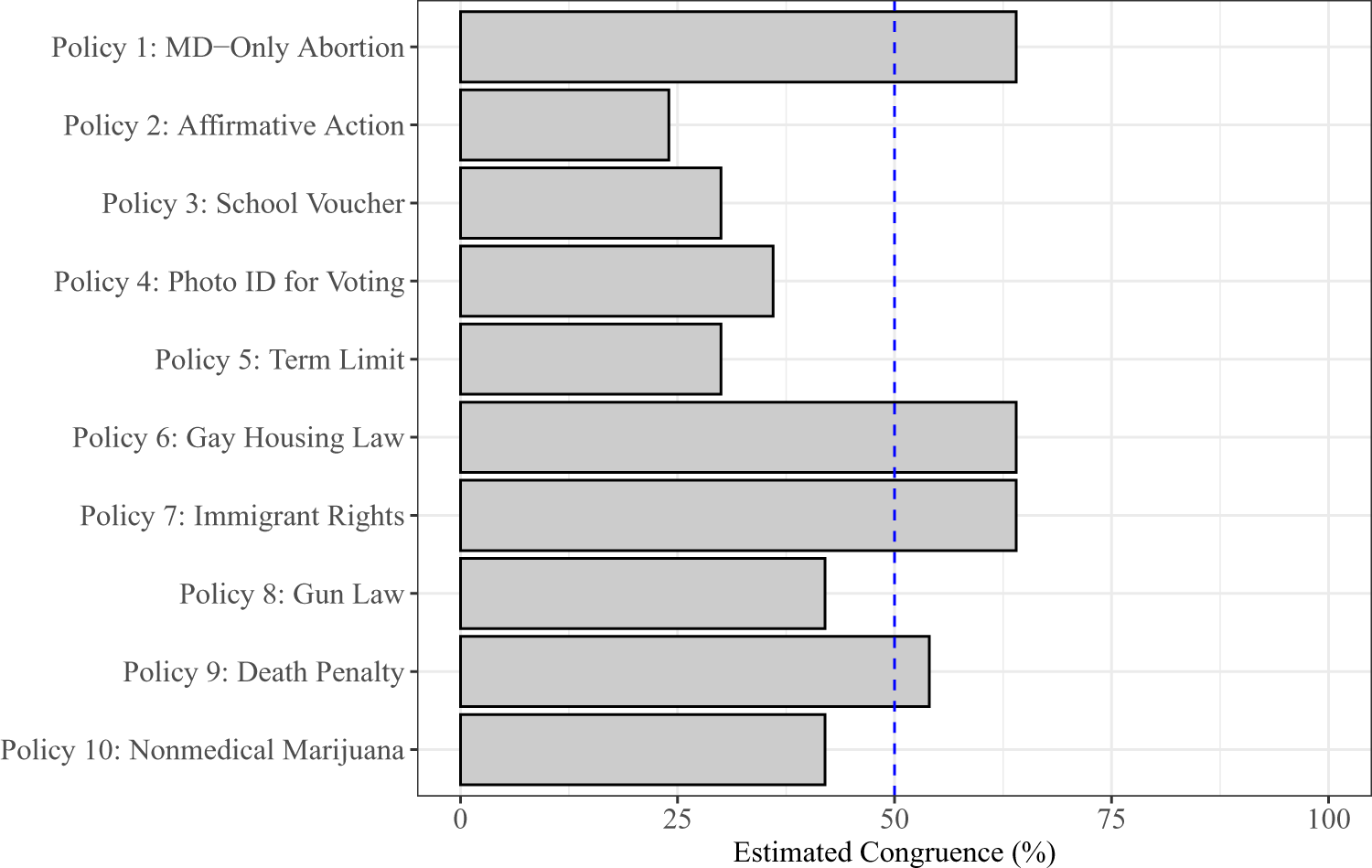
To test robustness, we take a different approach to account for preference intensity in our estimation of congruence.Footnote 14 This alternative approach determines the majority opinion among only respondents with intense preferences, identified based on the number of votes they cast on a particular policy. Specifically, we assume respondents who cast zero or one vote on a given policy as holding non-intense preferences toward that policy, and thus remove them from the analysis and use MRP to estimate the proportion of citizens who favored or opposed the policy in each of 50 states. Here, our use of MRP to estimate majority opinion resonates with Lax and Phillips (Reference Lax and Phillips2012); the difference is simply that while they use binary survey questions (e.g., “favor” or “oppose”) to gauge majority opinion, we use QVSR to measure majority support while discounting non-intense public opinion. Mapping these estimated state-level majority opinions (which account for preference intensity) onto actual policies across the American states, we continue to find low levels of congruence (Figure 3).
Estimated congruence across 10 policies, based on a measure that excludes non-intense individuals before calculating majority opinion.

Figure 3 Long description
Horizontal bar graph with 10 horizontal bars labeled on the left: Policy 1: MD dash Only Abortion; Policy 2: Affirmative Action; Policy 3: School Voucher; Policy 4: Photo ID for Voting; Policy 5: Term Limit; Policy 6: Gay Housing Law; Policy 7: Immigrant Rights; Policy 8: Gun Law; Policy 9: Death Penalty; Policy 10: Nonmedical Marijuana. Horizontal axis label: Estimated Congruence left parenthesis percent right parenthesis. Tick labels shown: 0, 25, 50, 75, 100. Vertical dashed reference line at 50. Bar endpoints on the horizontal scale: Policy 1 about 63 percent; Policy 2 about 24 percent; Policy 3 about 30 percent; Policy 4 about 36 percent; Policy 5 about 30 percent; Policy 6 about 63 percent; Policy 7 about 63 percent; Policy 8 about 42 percent; Policy 9 about 54 percent; Policy 10 about 42 percent.
To investigate further, rather than consider preference directionality and intensity jointly, we zero in on the independent role of preference intensity in shaping policy outcomes. We focus on all the state-policy observations for which there is narrow relative support for or opposition to a policy and test whether preference intensity per se predicts whether or not a given policy is implemented in a state. If preference intensity among the mass public plays an important role in influencing policymaking in the American states, we should observe that where the policies are closely contested in public opinion and get limited majority support from state residents, preference intensity strongly predicts policy adoption. This analysis is useful because it addresses the question of whether preference intensity matters in marginal cases where the policy receives narrow relative support or opposition in the state.
Our analysis takes three steps. First, we use QVSR– to identify policies that receive narrow relative support or opposition upon accounting for preference intensity in each state. For a given policy, we extract the MRP estimates based on QVSR– and operationalize policies backed by narrow relative support or confronted with narrow relative opposition in the state as those with MRP estimates ranging from  $-$0.1 to 0.1. For robustness, we also expand our operationalization of narrow relative support or opposition and consider alternative bandwidths (i.e.,
 $-$0.15 to 0.15,
 $-$0.2 to 0.2, and
 $-$0.25 to 0.25). Second, we estimate
 $|\text{Number of Votes for Policy } k_i|$, our measure of preference intensity that is largely insensitive to alternative policy bundles in our validation experiment, at the state level also by using MRP. Third, for each state-policy observation, we regress the policy adoption status, measured by whether or not the state policy is congruent with the preferences of a majority of the state’s survey respondents, on
 $|\text{Number of Votes for Policy } k_i|$ at the state level.
We report these results in columns 1–4 of Table 4, which show that state-level preference intensity does not have a significant positive correlation with policy adoption status across different bandwidths of public support. The relationship is statistically insignificant in all four specifications, and the point estimate is negative in two of the four specifications. We then address a limitation of this research design by including QVSR– as an additional covariate to capture the size of the majority in favor of a particular policy in a given state. Adding this covariate to the regression allows the probability of implementing a policy to vary linearly with the size of the majority in favor of the policy. In these specifications reported in columns 5–8 of Table 4, we again find that there is no significant relationship between preference intensity and the probability a state has the policy that a majority of its citizens prefer. The point estimates for the coefficient on  $|\text{Number of Votes for Policy } k_i|$ are all statistically insignificant, and in three of the four specifications the point estimates are in fact negative. By looking into state policies supported by narrow majorities and leveraging a novel measure of preference intensity, we provide additional empirical evidence that paints a less optimistic picture of policy representation in the United States. Recent but prominent speculations that preference intensity matters in US policymaking are therefore less consistent with our data at hand.
Preference intensity and policy congruence in marginal cases

Table 4 Long description
Eight OLS regression models estimate how state policy congruence relates to preference intensity (number of votes in the state, absolute) and, in models 5 to 8, mean QVSR in the state (absolute). The vote-count coefficient changes direction across specifications, ranging from about minus 0.80 (model 2) to plus 0.47 (model 4), with standard errors that are larger than the estimates in every model. Mean QVSR is negative in models 5 and 6 (about minus 2.73 and minus 1.58) but turns positive in models 7 and 8 (about 0.44 and 2.42), again with standard errors that are sizable relative to the coefficients. Intercepts vary from about minus 0.14 to 1.12 across models. Bandwidths widen from plus or minus 0.10 to plus or minus 0.25 across models 1 to 4 and 5 to 8, and the number of observations increases with wider bandwidths from 45 to 184. Overall, the pattern suggests no stable association between these predictors and policy congruence in these marginal-case samples, and the uncertainty is high.
Notes: OLS is the estimator. Number of votes in the states (absolute) is our novel measure of preference intensity as validated by our experiment (see Supplementary Appendix B). For logit estimates, see Table S17 in Supplementary Appendix J. Standard errors are reported in parentheses.
4. Conclusion
Individuals care about different issues to varying degrees. While preference intensity is central to theories of political behavior and policymaking, empirically assessing its importance has been difficult due to the scarcity of reliable measures of individuals’ preference intensity. In this article, we implemented an original national survey to measure preference intensity toward 10 very different policies that have direct correspondence to state laws and applied new estimates of public opinion to study policy representation in the American states. By mapping state-level preference intensity onto policy implementation status, we showed that while policy outcomes were generally responsive to public opinion (consistent with much of the existing literature), the overall level of policy congruence was quite low.
Given the existing literature that shows the lack of congruence in terms of preference directionality (e.g., Matsusaka, Reference Matsusaka2010; Lax and Phillips, Reference Lax and Phillips2012), our results provide fresh evidence that the lack of policy representation in the United States cannot be explained away by the existing scholarship’s failure to integrate preference intensity into the empirical analysis. This conclusion held across multiple measures of public opinion that reasonably accounted for preference intensity, including the standard Likert and “most important policy” items as well as the quadratic voting method. By explicitly incorporating the role of preference intensity and estimating policy congruence with new measures and new data that cover a wide range of policy issues, our analysis suggested that state policy outcomes in the United States are only weakly predicted by preference directionality and intensity of the state majorities. Therefore, we make a timely and important contribution to the literature on policy representation in American politics through a new empirical perspective.
Our careful attention to measurement also makes a methodological contribution to survey research. To validate the robustness of QVSR, we embedded an original experiment in our survey and used preregistered analytical procedures to demonstrate that QVSR measures of preference intensity, on average, were relatively insensitive to the particular choice sets that we offered—which spanned multiple typical issue areas such as abortion, education, and gay rights. While there were differences in the respondents’ assessment of the importance of the 10 policy issues in our study and while there were some small differences in the number of votes cast on a policy issue given the composition of the policy bundle, these differences did not dramatically affect the estimates of respondents’ preference intensity on average. These findings alleviate a significant but untested concern about QVSR regarding its sensitivity and contribute to the emerging literature that validates the use of QVSR in measuring preference intensity (Quarfoot et al., Reference Quarfoot, von Kohorn, Slavin, Sutherland, Goldstein and Konar2017; Cavaillé et al., Reference Cavaillé, Chen and Van der Straeten2019, Reference Cavaillé, Chen and Van der Straeten2025; Casella and Sanchez, Reference Casella and Sanchez2022). For applied researchers who seek to use measures of preference intensity for the same issue across multiple studies that may adopt distinct bundles of policy issues, these findings are reassuring and illustrate that these QVSR-derived measures of policy preferences can be comparable even when the policy bundles differ across studies.
4.1. Limitations and directions for future research
We recognize that our study was conducted on an opt-in Internet sample, which likely differs in unobservable characteristics from the US adult population. Although our sample demographics closely mirrored US adult population (Supplementary Appendix A), future research would benefit from replicating our analysis—for example, by using other survey platforms and modes—to further evaluate the sensitivity of the findings to other survey sampling approaches. To overcome the potential limitations of a non-representative sample, our observational analysis employed MRP to measure state-level policy preferences in order to correct for potential sampling bias within the US adult population and to generate valid state-level estimates (Wang et al., Reference Wang, Rothschild, Goel and Gelman2015; Downes et al., Reference Marnie, Gurrin, English, Pirkis, Currier, Spittal and Carlin2018; Kennedy and Gelman, Reference Kennedy and Gelman2021). One caveat, however, is that although our survey instrument appeared to successfully capture meaningful variations in preference intensity (see, e.g., Supplementary Appendix I.2), there was a lack of variations in state-level policy preferences in aggregate—even for Likert-based measures—among the 10 very specific policies we examined (see Supplementary Appendix F). Given these limitations, we acknowledge that our MRP analysis provides a proof of concept that invites future scholarship to further test the relationship between preference intensity and policy congruence with more representative samples and a wider set of policies. Because QVSR is nascent in the social sciences and its application remains scarce in substantive political science research (cf. Holland, Reference Holland2023; Kamphorst, Reference Kamphorst2024), there are potentially unknown assumptions and features of QVSR that await further validation by future scholarship, including what else QVSR-based measures might capture in addition to, or independent of, preference intensity (see Supplementary Appendix E for auxiliary analyses of QVSR’s additional properties). If resources—in terms of both sample size and survey length—permit, researchers may find it useful to advance understandings of policy representation by using not only QVSR but also conjoint experiments to measure preference intensity in mass publics (e.g.,Hanretty et al., Reference Chris, Lauderdale and Vivyan2020; Sides et al., Reference Sides, Tausanovitch and Vavreck2022).Footnote 15
In this study, we took advantage of the latest advances in survey methodology to investigate policy representation in the United States through a new empirical lens and yielded illuminating insights. Our study opens up exciting avenues for scholars to make—and empirically test—other important methodological and substantive inquiries. On the methodological side, examining the performance of alternative methods of preference elicitation, such as using a linear cost function as opposed to a quadratic cost function, may be a promising area of inquiry. Particularly, one potential explanation for the relative stability of the preference intensity measures is our use of the quadratic cost function as opposed to a linear cost function: by design, the marginal cost of casting an additional vote is increasing in the number of votes cast for the quadratic specification; this feature thus has the effect of tamping down elicited preference intensity relative to a linear cost function. On the substantive side, explaining variation in preference intensity across individuals and how preference intensity shapes the political process would be important, which future research can start to unpack by using our multidimensional measurement approach. Our analysis of responsiveness and congruence, based on data extracted from a one-time snapshot, was inherently static and devoid of contextual richness. But if the status quo for a given policy in a given state appears robust with little likelihood of reform, it is possible that individuals will not prioritize the issue when responding to the survey, even if they care about it intrinsically.Footnote 16 Given existing knowledge on how public opinion can evolve in dynamic political settings (e.g.,Chong and Druckman, Reference Dennis and Druckman2010; Yeung, Reference Yeung2025), future research would benefit immensely from studying policy representation not only by using data over time Caughey and Warshaw (Reference Caughey and Warshaw2022) but also by taking the role of measurement seriously.
Acknowledgements
We thank Nathalie Giger and two anonymous reviewers at PSRM for their rigorous feedback, which helped improve our paper significantly. All errors are our own.
Author contributions
Both authors developed the project’s conceptual framework, designed the survey instrument, and collected the data. E.S.F.Y. analyzed the data and wrote and revised the paper with support from Z.P.
Data availability statement
Replication data and code can be found in Harvard Dataverse: https://dataverse.harvard.edu/dataverse/PSRM.
Declaration of interests
None.
Ethics and consents
Before we fielded our survey, we obtained IRB approval from Emory University (IRB ID: STUDY00004573). All respondents were given detailed information about their rights as a survey participant and were required to give their consent before they began the survey. We confirm compliance with APSA’s Principles and Guidance for Human Subjects Research.
Funding statement
We acknowledge the Department of Political Science at Emory University for funding support.
Supplementary material
The supplementary material for this article can be found at https://doi.org/10.1017/psrm.2026.10122. To obtain replication material for this article, https://url.uk.m.mimecastprotect.com/s/sDv6CL866TPMzJ22IBfMfyIagT?domain=doi.org.




 Open access

