





Impact Statement
This work demonstrates how differentiable PDE solvers can be coupled with trainable components to improve physical closures while preserving the structure of the governing equations. The proposed strategy enables existing simulation tools to be integrated into gradient-based learning pipelines without redesigning the numerical framework, while ensuring that physical constraints remain embedded throughout training. Applied to the compressible Reynolds-averaged Navier–Stokes equations, the approach shows that data-driven corrections can be optimized consistently within complex simulation environments. More broadly, the methodology opens new perspectives for hybrid scientific computing approaches combining physical models and data-driven Machine Learning for a broad class of PDE-constrained problems.
1. Introduction
Partial differential equations (PDEs) are at the heart of mathematical modeling in physics and engineering. They describe how physical quantities such as temperature, pressure, and velocity in fluids evolve in space and time, encapsulating conservation laws such as those of mass, momentum, and energy. The complexity of these equations often renders analytical solutions intractable, especially in realistic geometries or in the presence of nonlinearities. As a result, numerical methods have become indispensable tools for solving PDEs, giving rise to a wide range of simulation frameworks across scientific disciplines.
From an engineering perspective, the development of Computational Fluid Dynamics (CFD) codes is crucial for predicting the forces needed to size and manufacture components, especially in high-performance applications such as turbines in jet engines. This process relies on advanced computational and experimental techniques to optimize performance.
The design of aerodynamic profiles is an iterative process, starting with data acquisition, followed by simulations and prototype testing to refine the design. Modern methods integrate optimization algorithms, more recently Machine Learning (ML) (Wu et al., Reference Wu, Xiao and Paterson2018; Ströfer and Xiao, Reference Ströfer and Xiao2021), to balance aerodynamics, thermodynamics, and structural mechanics, improving the overall design.
In recent years, ML has gained increasing attention as a powerful tool in applied mathematics, particularly for problems traditionally addressed through numerical analysis. Recent works have investigated the integration of ML directly into the numerical discretization of Finite Volume (FV) solvers. Data-driven learned discretizations for hyperbolic conservation laws have been proposed to replace classical gradient or flux reconstructions with Neural Networks (NNs) trained on high-resolution data, achieving improved accuracy on coarse meshes and in the presence of shocks (Romémont et al., Reference Romémont, Renac, Nunez and Chinesta2026). These approaches effectively modify the internal structure of the CFD solver itself and are typically implemented (including the PDE solver) in dedicated ML-based frameworks. More generally, structure-preserving neural architectures such as volume-preserving transformers have been introduced to ensure stability and long-term consistency in learned dynamical systems (Brantner et al., Reference Brantner, Kraus, Li and de Romemont2025).
ML’s flexibility in approximating complex functions has led to the development of surrogate models (Kutz, Reference Kutz2017; Casenave et al., Reference Casenave, Roynard, Staber, Piat, Bucci, Akkari, Kabalan, Nguyen, Saverio, Perez, Kalaydjian, Fouché, Gonon, Najjar, Menier, Nastorg, Catalani and Rey2025; Catalani et al., Reference Catalani, Fesquet, Bertrand, Tost, Bauerheim and Morlier2026) that can either completely replace or be integrated into and used to accelerate classical solvers, especially when repeated evaluations are required, such as in (shape) optimization or uncertainty quantification. Beyond surrogate modeling, ML techniques have also been used to correct or augment existing numerical models by learning discrepancies between model predictions and high-fidelity data. In the context of PDEs, NNs have been employed both to represent solutions directly, as in Physics-Informed Neural Networks (PINNs) (Raissi et al., Reference Raissi, Perdikaris and Karniadakis2019), and to infer hidden physical quantities or closure terms, offering new paradigms for solving inverse problems or discovering governing laws from data (Ströfer and Xiao, Reference Ströfer and Xiao2021). These approaches open new perspectives for hybrid modeling strategies that combine domain knowledge with data-driven learning.
CFD mainly focuses on solving the Navier–Stokes (NS) equations to study the behavior and interactions of fluids. Specifically, for turbulent flows, the Reynolds-averaged Navier–Stokes (RANS) equations introduce turbulence models to close the system, each model representing a compromise between fidelity and computational feasibility. The choice and accuracy of these turbulence models critically influence the reliability of CFD simulations, especially in the design and optimization of high-performance components.
The accurate simulation of turbulent flows remains one of the major challenges in CFD. Traditional RANS models provide a cost-efficient approach by introducing closure relations for the Reynolds stresses, yet their performance strongly depends on empirical assumptions and model calibration. Classical turbulence closures, such as the
$ k $
 –
$ \varepsilon $
 ,
$ k $
 –
$ \omega $
 , and Spalart–Allmaras (SA) models (Pederson, Reference Pederson2025), while robust and computationally efficient, are known to fail in the prediction of separated or highly anisotropic flows.
The closure modeling problem is a generic feature of nonlinear multiscale PDE systems, arising whenever a reduced or averaged description is sought. A closely related viewpoint emerges in data assimilation, where the full state of a nonlinear multiscale system is reconstructed from partial observations by solving an inverse problem, typically through the introduction of correction or control terms. In variational approaches, these corrections are adjusted to enforce consistency between the model and the data (Talagrand, Reference Talagrand1997). From this perspective, data assimilation can be interpreted as an implicit closure strategy, in which the inferred corrections encode the effects of unresolved scales or model errors; once learned or parameterized as functions of the resolved state, they can be recast as explicit closure models, thereby bridging inverse problems and reduced-order modeling. Duraisamy et al. (Reference Duraisamy, Iaccarino and Xiao2019) provided a comprehensive overview of data assimilation (field-inversion) and ML-augmented RANS modeling, highlighting the opportunities and difficulties in integrating data-driven corrections within physics-based solvers. Furthermore, a more recent view made by Girimaji (Reference Girimaji2024) emphasized that, despite the promising results, ML-driven turbulence modeling must still tackle issues of generalization, interpretability, and physical consistency.
In the literature, various ML-based approaches have been proposed to enhance RANS closures (Zhao et al., Reference Zhao, Akolekar, Weatheritt, Michelassi and Sandberg2020; Zhu et al., Reference Zhu, Zhang and Tu2021). For instance, Sanhueza et al. (Reference Sanhueza, Smit, Peeters and Pecnik2023) employed NNs to model the effects of variable fluid properties on turbulence transport, while Chen and Deng (Reference Chen and Deng2024) trained data-driven closures for the
$ k $
 –
$ \omega $
 SST model, learning discrepancies between RANS and high-fidelity data to improve mean-field predictions. Aly (Reference Aly2024) introduced a Deep Learning (DL) model to predict the eddy viscosity field, training directly on the eddy viscosity, yet still achieving improved accuracy in bluff-body simulations, opening the way for turbulent viscosity prediction using NNs. Surrogate modeling has also been applied to turbulence closure; for instance, Schlichter et al. (Reference Schlichter, Reck, Pieringer and Indinger2024) benchmarked surrogate models for RANS closures based on the
$ k $
 –
$ \omega $
 SST model.
Despite the progress, most of these methods treat the ML model as an external correction or surrogate, rather than embedding it within an end-to-end differentiable simulation pipeline, as done in Ströfer and Xiao (Reference Ströfer and Xiao2021). In addition, most ML-RANS studies rely on incompressible solvers. This preference arises because, in the incompressible regime, the Reynolds stress tensor admits an exact decomposition following Pope (Reference Pope1975), as commonly exploited in recent works (Ströfer and Xiao, Reference Ströfer and Xiao2021; Zhang et al., Reference Zhang, Xiao, Jee and He2023). Furthermore, the incompressible NS equations admit a continuous adjoint formulation, which substantially simplifies the derivation and computation of adjoint-based gradients.
A complementary line of research has explored the use of Graph Neural Networks (GNNs) as data-driven correction models defined directly on unstructured computational meshes. Recent works by Quattromini et al. have proposed physics-constrained GNN architectures for mean-flow reconstruction and data assimilation in CFD (Quattromini et al., Reference Quattromini, Bucci, Cherubini and Semeraro2025a, Reference Quattromini, Bucci, Cherubini and Semeraro2025b). In these methods, the GNN is trained to predict the forcing or closure term that brings a baseline RANS or mean-flow solution into agreement with high-fidelity or experimental data. The graph-based formulation naturally accommodates arbitrary mesh connectivity and allows the use of solver-derived sensitivities during training.
Industrial CFD codes are typically developed over time spans of 10–20 years within High-Performance Computing (HPC) environments, often consisting of Python interfaces wrapped around legacy Fortran or C++ kernels to ensure high performance on large clusters. It is, therefore, desirable to design a pipeline that enables seamless integration of such CFD solvers with modern ML frameworks like PyTorch, as similarly done by Atkinson et al. (Reference Atkinson, Elafrou, Kasoar, Wallwork, Meltzer, Clifford, Orchard and Edsall2025).
In the context considered in this work, the PDE solver—specifically a CFD solver—must be treated as a standard PyTorch module, supporting both forward and backward differentiation. At the same time, we aim to preserve the mature, highly optimized numerical algorithms already available in industrial CFD codes—for example, Newton-based nonlinear relaxation schemes and preconditioned GMRes methods (Saad and Schultz, Reference Saad and Schultz1986) for large-scale linear systems. This motivates handling the CFD solver as an implicit layer within PyTorch, with full support for automatic differentiation in both directions.
Furthermore, we aim to introduce ML operators, such as NNs, in an end-to-end structure inside the CFD-PyTorch module. Therefore, once the parameters, or the NN, have been trained, we would still like to rely on the dedicated algorithms embedded in the CFD code to solve the resulting hybrid PDE–ML system efficiently. This requires incorporating the contributions of the trainable model component directly into the Jacobian used for implicit time integration or steady-state solution. The present paper introduces a pipeline that fulfills these objectives.
Unlike PINN approaches, where the solution of the PDE is directly represented by a NN and learned through the minimization of the governing-equation residuals, the present framework relies on an existing differentiable PDE solver to compute the discrete physical state. The proposed methodology, therefore, preserves the original numerical discretization and solution strategy of the selected solver. Depending on the considered formulation, the governing equations may either be enforced weakly through residual minimization, similarly to PINN strategies, or solved directly in strong form through an implicit-layer formulation. In both cases, gradients are propagated through the numerical solver itself using implicit differentiation. This enables the integration of ML models into established simulation frameworks without replacing the underlying numerical methodology.
The originality of the present work lies not in the use of differentiable programming itself, but in the construction of a practical end-to-end framework coupling classical PDE solvers, implicit differentiation techniques, and trainable closure models within large-scale CFD applications.
Here, we demonstrate the approach by coupling PyTorch with the compressible CFD solver BROADCAST (Poulain et al., Reference Poulain, Content, Sipp, Rigas and Garnier2023), which typifies industrial CFD codes built around a Python interface wrapping Fortran kernels. Algorithmic differentiation (AD) is performed using the software Tapenade (Hascoët, Reference Hascoët2004), enabling efficient evaluation of vector–Jacobian products at a reasonable computational cost (Maugars et al., Reference Maugars, Bourasseau, Content, Michel, Berthoul, Ramirez, Raud and Hascoët2022). This capability is essential for the practical implementation of adjoint-based optimization.
NNs are adopted as ML models due to the universal approximation theorem, which guarantees their ability to approximate a broad class of nonlinear functions. In addition, NNs can be efficiently trained using gradient-based optimization methods. Their capability to handle heterogeneous datasets, together with their flexibility and generality, makes them a robust and widely applicable strategy for processing and predicting data arising from numerical simulations. This approach bridges the gap between physics-based solvers and data-driven learning, extending ML-RANS methodologies toward fully integrated optimization pipelines for aerodynamic design.
This pipeline is applied to the improvement of turbulence models for the RANS equations. In this setting, we introduce an end-to-end differentiable framework that couples the BROADCAST compressible RANS solver with PyTorch, enabling the optimization of NN weights directly within the solver. This approach allows turbulence quantities, such as the eddy viscosity, to be optimized through algorithmic differentiation, thereby providing a fully consistent and automated route for data-driven closure modeling.
The pipeline is first tested on the 2D NASA Wall-Mounted Hump separated flow (Jespersen et al., Reference Jespersen, Pulliam and Childs2016; Pederson, Reference Pederson2021) to optimize a control parameter in the production term of the transport equation of the turbulent variable of the SA model (Cato et al., Reference Cato, Volpiani, Mons, Marquet and Sipp2023; Fanizza et al., Reference Fanizza, Volpiani, Renac, Martin and Sipp2025). Subsequently, to further explore the capabilities of the framework, it is applied to the VKI LS-59 turbine blade case (Hercus and Cinnella, Reference Hercus and Cinnella2011) with transonic flow to perform an optimization directly on the eddy viscosity and finally on a dataset generated starting from the benchmark case. This comprehensive approach aims to enhance the predictive accuracy of turbulence models, thereby contributing to more efficient and reliable aerodynamic simulations.
The structure of this paper is as follows. First, the general formulation of the tackled PDEs is introduced, together with a discussion of their abstract representation and closure requirements (§ 2). Next, the proposed optimization framework is described, outlining the possible objective functions and distinguishing between cases where the full-state variable is available and cases where it is unknown and must be computed (§ 2.2). The specific problem under investigation is then presented as a benchmark to demonstrate the capabilities of the developed framework, followed by a detailed presentation of the CFD equations in use and closure models (§ 3.1). Subsequently, the technical implementation is discussed, with particular emphasis on the PyTorch-based routines and the design of custom differentiable modules (§ 3.4). The application cases are presented by first describing the considered geometries and then the adopted optimization strategies (§ 4). The generation of the training dataset is described, with particular emphasis on the variations in geometry and flow conditions (§ 4.4.1). Each case is followed by a detailed presentation and analysis of the results obtained with the different approaches. Finally, conclusions are drawn and perspectives for future developments are outlined.
2. Enhancing partial differential equations resolution using machine learning
We start by considering a baseline model consisting of a system of nonlinear PDEs defined over a spatial domain
$ \Omega $
 , written in compact form as
$ \mathcal{R}\left(\boldsymbol{\omega} \right)=0 $
 , where
$ \boldsymbol{\omega} $
 denotes the state variables of interest. Discretization on a mesh using Finite Difference (FD), Finite Element (FE), or FV methods leads to a system
$ \boldsymbol{R}\left(\boldsymbol{w}\right)=0 $
 , where
$ \boldsymbol{w} $
 represents the discretized state. Although the methodology is general, the implementations considered in this work rely on structured meshes, mainly to exploit the sparsity structure of the numerical operators, as discussed in Section 3.4. For instance, with a FV method with
$ m $
 variables on a structured mesh of size
$ {n}_i\times {n}_j $
 , the total number of degrees of freedom of the state
$ N=m\times {n}_i{n}_j $
 . To enhance the model accuracy, a discrete additive correction term
$ \boldsymbol{f}\left(\boldsymbol{w}\right)={\boldsymbol{f}}_{\boldsymbol{\vartheta}}\left(\boldsymbol{w}\right) $
 , parameterized by coefficients
$ \boldsymbol{\vartheta} $
 , is introduced. These parameters are determined by minimizing an objective functional
$ \mathcal{J}\left(\boldsymbol{w}\right) $
 , defined, for instance, from sparse experimental observations or high-fidelity reference data.
Then, the hybrid discrete model can be written as follows:

where
$ \boldsymbol{w}\in {\unicode{x211D}}^N $
 ,
$ \boldsymbol{R}\left(\boldsymbol{w}\right):{\unicode{x211D}}^N\to {\unicode{x211D}}^N $
 , and
$ {\boldsymbol{f}}_{\boldsymbol{\vartheta}}\left(\boldsymbol{w}\right):{\unicode{x211D}}^N\to {\unicode{x211D}}^N $
 . Although the target solution is steady, an implicit pseudo-time integration scheme is considered to iteratively converge toward the steady solution. Here, the implicit time discretization scheme of the hybrid model is assumed to be:

On the other hand, the correction
$ {\boldsymbol{f}}_{\boldsymbol{\vartheta}}\left(\boldsymbol{w}\right) $
 may represent either a local or a nonlocal closure. In the local case, it can be written as
$ {\boldsymbol{f}}_{\boldsymbol{\vartheta}}\left(\boldsymbol{w}\right)=\boldsymbol{f}\left(\boldsymbol{w},{\boldsymbol{\alpha}}_{\boldsymbol{\vartheta}}\circ \boldsymbol{\phi} \left(\boldsymbol{w}\right)\right) $
 , where
$ \boldsymbol{\phi} \left(\boldsymbol{w}\right) $
 denotes a set of local features and
$ {\boldsymbol{\alpha}}_{\boldsymbol{\vartheta}} $
 is a parametric mapping that returns a local correction field
$ \boldsymbol{\alpha} $
 . In the nonlocal case, the correction takes the form
$ {\boldsymbol{f}}_{\boldsymbol{\vartheta}}\left(\boldsymbol{w}\right)=\boldsymbol{f}\left(\boldsymbol{w},{\boldsymbol{\alpha}}_{\boldsymbol{\vartheta}}\left(\boldsymbol{w}\right)\right) $
 , where
$ {\boldsymbol{\alpha}}_{\boldsymbol{\vartheta}} $
 depends on the global or neighborhood state and can therefore capture nonlocal interactions between cells. In practice,
$ {\boldsymbol{\alpha}}_{\boldsymbol{\vartheta}} $
 may be instantiated, for instance, as a MultiLayer Perceptron (MLP) in the local setting or as a GNN in the nonlocal one, although the present formulation remains independent of the specific choice of parametrization.
In this section, we address two algorithmic problems that combine a PDE solver and trainable parameters. First (§ 2.1), for given parameters
$ \boldsymbol{\vartheta} $
 , we seek the state
$ \boldsymbol{w} $
 that solves (2.1), or:

This requires adapting the solution strategies of the PDE solver underlying
$ \boldsymbol{R} $
 so that the correction term
$ {\boldsymbol{f}}_{\boldsymbol{\vartheta}}\left(\boldsymbol{w}\right) $
 is properly taken into account.
Second (§ 2.2), for a given cost functional
$ \mathcal{J}\left(\boldsymbol{w},\boldsymbol{\vartheta} \right) $
 , we seek parameters
$ \boldsymbol{\vartheta} $
 such that

The objective is to optimize the weights
$ \boldsymbol{\vartheta} $
 (e.g., within PyTorch), and the key question becomes: what functionalities must the PDE code
$ \boldsymbol{R}\left(\boldsymbol{w}\right) $
 provide to enable transparent and smooth forward and backward propagations through the PDE solver?
2.1. Solving for the state for fixed parameters
For context, it is important to stress that in DL, models are typically constructed as compositions of elementary explicit functions, called layers, where each layer produces its output from its input through a closed-form evaluation. In contrast, the solution of PDEs often relies on the numerical solution of implicit nonlinear systems, where the state is defined as the solution of a residual equation rather than by an explicit formula. This fundamental difference motivates the introduction of implicit operators within differentiable learning frameworks, as done in Bai et al. (Reference Bai, Kolter and Koltun2019). Having defined the concepts of explicit and implicit layers, given a fixed set of parameters, the hybrid problem (2.1) can be solved either by a residual minimization technique (an explicit operation) or a Newton-like relaxation method (an implicit system).
2.1.1. Residual minimization with an explicit layer
The first strategy to solve problem (2.1) avoids forming the Jacobian explicitly by recasting the state solve as a residual minimization problem. In this formulation, the state is obtained by minimizing the norm of the residual, typically through an iterative method that requires only the evaluation of the residual itself and back-propagation through the PDE solver
$ {\left({\partial}_{\boldsymbol{w}}\boldsymbol{R}\right)}^{\top } $
 and through the closure term
$ {\left({\partial}_{\boldsymbol{w}}{\boldsymbol{f}}_{\boldsymbol{\vartheta}}\right)}^{\top } $
 . Then, the functional to be minimized is fixed as follows:

and the differential of
$ \mathcal{J}\left(\boldsymbol{w}\right) $
 can be computed as follows:

where
$ \parallel \cdot {\parallel}_Q^2={\left\langle \cdot, \cdot \right\rangle}_Q $
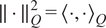 and
$ {\left\langle {\boldsymbol{w}}_1,{\boldsymbol{w}}_2\right\rangle}_Q={\boldsymbol{w}}_1^{\top }{\boldsymbol{Qw}}_2 $
 are the discrete inner product and
$ \boldsymbol{Q}\in {\unicode{x211D}}^{N\times N} $
 is a symmetric positive-definite matrix defining this discrete inner product in the state space. In practice,
$ \boldsymbol{Q} $
 involves the continuous
$ {L}^2 $
 inner product and accounts for the mesh discretization and for the relative scaling of the different state variables. For instance, in a FV discretization,
$ \boldsymbol{Q} $
 can be chosen as a diagonal matrix containing the cell volumes repeated for each state variable. This definition ensures that the residual norm corresponds to a physically meaningful weighted
$ {L}^2 $
 norm over the computational domain.
The forward and backward operators can be sketched as follows:


where all boxes, handled by a combination of the PDE solver and the automatic differentiation framework (e.g., PyTorch), are explicit since only explicit evaluation operations are involved.
Such an approach is conceptually related to PINNs (Raissi et al., Reference Raissi, Perdikaris and Karniadakis2019), in the sense that the solution is obtained through the minimization of the governing-equation residuals. In addition, it reduces the memory footprint (there is no matrix to invert) and simplifies the implementation, making it attractive when the Jacobian is difficult or expensive to compute. However, it may converge more slowly than Newton-type schemes, and its efficiency depends on the choice of minimization algorithm and the conditioning of the residual landscape.
2.1.2. Relaxation method with an implicit layer
As an alternative, problem (2.1) may be solved iteratively by the following relaxation method:

The pseudo time-step
$ \Delta t $
 is small at the beginning of the iterations to accommodate for the initial condition, and then it increases to reach
$ \Delta t\to \infty $
 , where we recover the quadratic convergence properties of the Newton method (Polyak, Reference Polyak2007). The pseudo time-step
$ \Delta t $
 can be derived from an adaptive stability criterion that evolves with the residual norm, see, for example, Crivellini and Bassi (Reference Crivellini and Bassi2011) in the case of advection dominated systems with the local
$ CFL=c\Delta t/\Delta x $
 condition (
$ \Delta x $
 is the local mesh size and
$ c $
 is the speed of the fastest waves). Note that using a Newton strategy requires the full Jacobian
$ {\partial}_{\boldsymbol{w}}\boldsymbol{R}+{\partial}_{\boldsymbol{w}}{\boldsymbol{f}}_{\boldsymbol{\vartheta}} $
 to be invertible at the targeted fixed point, which excludes being in the vicinity of saddle-node, pitchfork, or transcritical bifurcation thresholds.
This method requires assembling and inverting the sparse Jacobian by exploiting the stencil-based independence of the numerical scheme. The sparsity pattern of the Jacobian is inferred from the discretization stencil, allowing the use of directional test vectors to probe multiple independent degrees of freedom simultaneously. As a consequence, several Jacobian entries are computed at once using the same test vector, and the corresponding matrix-vector products are performed in parallel, resulting in an efficient sparse assembly procedure.
The Jacobian can be decomposed into two contributions: the part associated with the PDE solver,
$ {\partial}_{\boldsymbol{w}}\boldsymbol{R} $
 , and the component arising from the linearization of the ML model,
$ {\partial}_{\boldsymbol{w}}{\boldsymbol{f}}_{\boldsymbol{\vartheta}} $
 . When
$ {\boldsymbol{f}}_{\boldsymbol{\vartheta}} $
 is represented by, or contains, a NN, it is essential that the spatial support (or receptive field) of its linear operations does not exceed the stencil width of the underlying numerical scheme. Otherwise, additional couplings would be introduced beyond the assumed sparsity pattern, leading to an incorrect Jacobian structure. This aspect is further discussed in Appendix D. To relax the constraints on the NN architecture, matrix-free methods could be considered. However, their convergence is typically more challenging without ad hoc preconditioning. This aspect could be explored in future works.
Both methods, explicit and implicit, are compatible with the differentiable framework used in this work, and the choice between them depends on the trade-off between computational cost, implementation complexity, and convergence properties.
2.2. Optimization framework
We aim at optimizing the parameters
$ \boldsymbol{\vartheta} $
 of a correction term
$ {\boldsymbol{f}}_{\boldsymbol{\vartheta}}\left(\boldsymbol{w}\right) $
 . Similar to how we previously introduced
$ \boldsymbol{Q} $
 , we introduce a symmetric positive-definite matrix
$ \boldsymbol{M} $
 defining the natural inner product in the parameter space:

Two classical situations arise:
-
1. In the case of data assimilation, we assume

meaning that the correction
$ {\boldsymbol{f}}_{\boldsymbol{\vartheta}} $
 is a function of a volumetric source term
$ \boldsymbol{\alpha} $
 defined on the computational mesh and handled by the discretization of a continuous operator. In such a case,
$ \boldsymbol{\vartheta} =\boldsymbol{\alpha} $
 and the scalar product
$ \boldsymbol{M} $
 may be chosen to discretize the continuous
$ {L}^2 $
 inner product, consistently with the inner product used for the state variables.
-
2. In the case of closure, we assume that

meaning that the correction
$ {\boldsymbol{f}}_{\boldsymbol{\vartheta}}\left(\boldsymbol{w}\right) $
 is a function of the above-introduced parameter
$ \boldsymbol{\alpha} $
 , which now depends on the state
$ \boldsymbol{w} $
 via a parametric model with parameters
$ \boldsymbol{\vartheta} $
 ,
$ {\boldsymbol{\alpha}}_{\boldsymbol{\vartheta}}\left(\boldsymbol{w}\right) $
 . In this case, the natural choice for the scalar product is
$ \boldsymbol{M}=\boldsymbol{I} $
 , since these parameters are not associated with a spatial discretization. Note that:


in which all derivatives are handled by the PDE solver, except for
$ {\partial}_{\boldsymbol{\vartheta}}\boldsymbol{\alpha} \left(\boldsymbol{w}\right) $
 , which is treated by the automatic differentiation framework (e.g., PyTorch), as it corresponds to the differentiation of the ML model.
2.2.1. Full-state
$ \boldsymbol{w}={\boldsymbol{w}}_m $
 and explicit layer

In this section, the full-state variable
$ \boldsymbol{w} $
 is assumed to be known at the training stage,
$ \boldsymbol{w}={\boldsymbol{w}}_m $
 . For example, this would be the case if a high-fidelity solver were used to obtain the training data. The optimization problem (2.4) may then be simplified and replaced by minimizing a cost-functional based on the residue:

The gradient of the cost-functional can then be obtained straightforwardly:

When using an optimizer based on the
$ {L}^2 $
 norm, it is essential that the gradient supplied to it lives in a Euclidean space. This inconsistency may result in suboptimal convergence, unstable optimization steps, or biased updates of the parameters. Hence, if
$ \boldsymbol{M}\ne I $
 , we need to introduce the variable
$ \tilde{\boldsymbol{\vartheta}}=\boldsymbol{N}\boldsymbol{\vartheta } $
 , where
$ \boldsymbol{M}={\boldsymbol{N}}^{\top}\boldsymbol{N} $
 (Cholesky decomposition of a symmetric positive definite matrix), so that

where the subscript
$ {}_2 $
 refers to the Euclidean norm. The correct gradient to be supplied to the Euclidean optimizer may then be obtained through:

In the present case, if
$ \boldsymbol{\vartheta} $
 represents the weights of a neural operator, the forward and backward operators can be sketched as follows:


where the boxes are handled by a combination of the PDE solver and the automatic differentiation framework. All layers are explicit in the present case since simple (explicit) evaluation operations are involved in all boxes.
2.2.2. Partial-state and implicit layer
In the case where the full-state variable
$ \boldsymbol{w} $
 is not known but only partial-state information collected in a cost functional
$ \mathcal{J}\left(\boldsymbol{w}\right) $
 is available, we can directly tackle the optimization problem in (2.4) by considering the Lagrangian:

The Karush–Kuhn–Tucker (KKT) optimality conditions are obtained by setting the derivatives with respect to the direct state
$ \boldsymbol{w} $
 and the adjoint state
$ \boldsymbol{\lambda} \in {\unicode{x211D}}^N $
 of the Lagrangian to zero:


then, having computed the solution
$ \boldsymbol{w} $
 of (2.22), we can use it to compute the Lagrange multiplier from (2.23). Finally, by substituting
$ \boldsymbol{\lambda} $
 in (2.24), it is possible to solve for the optimal value of
$ \boldsymbol{\vartheta} $
 with a gradient descent strategy, where the gradients are computed as follows:

where
$ \boldsymbol{M} $
 is again the natural inner product depending on the nature of the optimized parameters
$ \boldsymbol{\vartheta} $
 .
In the present case, the forward and backward operators of the considered implicit layer can be sketched as follows:


The boxes are handled by the PDE solver and the automatic differentiation framework, the underlined ones containing implicit operations (involving complex operations such as a Newton solver or a large-scale matrix inverse), the others being completely explicit. We insist on the fact that the underlined box in the backward operator is implicit: the operator
$ {\left({\partial}_{\boldsymbol{w}}\boldsymbol{R}+{\partial}_{\boldsymbol{w}}{\boldsymbol{f}}_{\boldsymbol{\vartheta}}\right)}^{-\top } $
 should not be interpreted as the application of the explicit inverse of the adjoint matrix (which is generally dense and cannot be stored). Instead, it corresponds to solving the linear system involving the adjoint matrix:

which can be done with either direct methods (e.g., with sparse LU methods Amestoy et al., Reference Amestoy, Buttari, L’Excellent and Mary2019; Amestoy et al., Reference Amestoy, Duff, Koster and L’Excellent2001) or iterative strategies (Fanizza et al., Reference Fanizza, Volpiani, Renac, Martin and Sipp2025). The adjoint system inherits the same sparsity pattern as the Jacobian arising from the linearization of the baseline PDE operator, and its eigenvalues and condition number remain unchanged with respect to the original system. Hence, from a mathematical point of view, the complexity in solving the adjoint system should be equivalent to solving the direct one.
In the case where
$ \boldsymbol{\vartheta} $
 designates a volumetric source term in the PDE solver, one needs, as in the previous section, to move to a Euclidean space by introducing the variable
$ \tilde{\boldsymbol{\vartheta}} $
 (see § C).
2.3. The end-to-end differentiable learning pipeline
Thanks to its flexibility, native support for automatic differentiation, and strong integration with scientific computing libraries, PyTorch (Paszke et al., Reference Paszke, Gross, Chintala, Chanan, Yang, DeVito, Lin, Desmaison, Antiga and Lerer2017) was selected as the core framework for implementing the computational routines developed in this work. The overall pipeline is organized around a modular structure composed of three fundamental components responsible for (i) enforcing boundary conditions, (ii) evaluating the discrete residual of the governing equations, and (iii) applying external or model-derived forcing terms. This layered design provides a clean interface between high-level Python code and low-level numerical kernels while ensuring that each stage of the computation remains physically consistent and computationally efficient.
A central requirement of this architecture is full differentiability. To achieve this, each component is implemented by overriding the forward and backward operations, through PyTorch’s torch.autograd.Function interface (It is also possible to define the Jacobian-vector product (jvp) inside a torch.autograd.Function, although it is not needed for optimization purposes; it may, however, be useful to construct the Jacobian for a Newton method.). This mechanism allows complex, optimized numerical routines to be embedded inside a differentiable computational graph while remaining fully compatible with PyTorch’s automatic differentiation engine.
The computational flow proceeds by sequentially applying the boundary-condition layer to the input state, evaluating the discrete residual of the governing equations, and finally incorporating the forcing contribution. By composing these custom layers into a standard PyTorch nn.Module, the framework automatically manages gradient propagation and the definition of the backward pass, enabling seamless integration with optimization algorithms and ML architectures.
To solve the nonlinear system associated with the discretized equations, the full computation is embedded within an outer layer implementing a Fixed-Point (FP) or Newton-type iteration strategy. This external layer overrides PyTorch’s default backward behavior by solving an associated adjoint system to compute exact gradients with respect to the trainable parameters. This ensures consistent gradient flow across iterative solves and enables end-to-end learning constrained by general nonlinear governing equations.
While the present work focuses on turbulence modeling within the RANS framework, as detailed in the following section, the abstract structure introduced in (2.1) is in fact representative of a much broader class of physical problems. In reactive flows, for instance, the correction term
$ \boldsymbol{f}\left(\boldsymbol{w}\right) $
 may account for source terms arising from chemical reactions. In porous media, it can represent Darcy-type drag effects, while in radiation or multiphase transport, it may encode closure relations for interfacial fluxes or effective material properties. Comparable formulations also emerge in solid mechanics, particularly in the constitutive modeling of complex materials. More generally, this work addresses the modeling of multiscale systems, where similar challenges arise across a wide range of physical contexts. In kinetic theory, such difficulties appear through moment hierarchies derived from the Boltzmann equation (Chapman and Cowling, Reference Chapman and Cowling1990). They are also central to many-body statistical physics via the BBGKY hierarchy (Huang, Reference Huang2008) and to solid mechanics through homogenization techniques and the derivation of effective constitutive laws (Torquato, Reference Torquato2002). From this perspective, the methodology proposed here can be viewed as a general strategy for incorporating modeling closures into PDE-based systems in a systematic and flexible manner. By leveraging differentiable solvers together with adjoint-based optimization, it enables a consistent and scalable coupling between physics-based models and trainable components. As such, it provides a natural framework for integrating ML into scientific computing workflows governed by PDEs, with potential applications well beyond turbulence modeling.
3. Data assimilation and closure with compressible RANS equations
In this section, we present the PDE problem under investigation and illustrate how the proposed pipeline can be applied to it. First (§3.1), we present the compressible RANS equations, before we introduce a data assimilation and closure problem with two possible tunable parameters: the eddy viscosity
$ {\mu}_t $
 (§3.2) and the production term
$ \beta $
 of the turbulent variable equation (§3.3).
3.1. Compressible RANS equations with Boussinesq hypothesis
The steady compressible RANS equations can be written as follows:

where the density
$ \rho $
 , pressure
$ p $
 , viscous stress tensor
$ \boldsymbol{\tau} $
 , and heat flux
$ \boldsymbol{q} $
 are Reynolds-averaged quantities, while the velocity vector
$ \boldsymbol{U}=\left[U,V\right] $
 and the total energy
$ E $
 are Favre-averaged quantities, defined through density-weighted averaging (Wilcox, Reference Wilcox2006). Finally,
$ {\boldsymbol{\tau}}^R $
 and
$ {\boldsymbol{q}}_t $
 denote the Reynolds stress tensor and the turbulent heat flux, respectively.
To close the system, models relating
$ {\boldsymbol{\tau}}^R $
 and
$ {\boldsymbol{q}}_t $
 to the state variables are required. Most commonly used approaches rely on the Boussinesq eddy viscosity assumption (Boussinesq, Reference Boussinesq1877), which states that the Reynolds stress tensor
$ {\boldsymbol{\tau}}^R $
 is proportional to the deviatoric part of the mean strain-rate tensor
$ \boldsymbol{S} $
 , with proportionality coefficient given by the eddy viscosity
$ {\mu}_t $
 . This yields:

where
$ {\mathit{\Pr}}_t $
 is the (constant) turbulent Prandtl number and
$ T $
 is the Reynolds-averaged temperature. As discussed in Wilcox (Reference Wilcox2006), a constant turbulent Prandtl number,
$ {\mathit{\Pr}}_t=0.9 $
 , is used in the present simulations and is considered an acceptable baseline choice for the adiabatic configurations investigated here. Then, by incorporating (3.2) in (3.1), the system reads:

After discretizing these equations, we consider two possible choices for the corrected model, characterized by different state variables
$ \boldsymbol{w} $
 , governing equations
$ \boldsymbol{R}\left(\boldsymbol{w}\right) $
 , and correction terms
$ {\boldsymbol{f}}_{\boldsymbol{\vartheta}}\left(\boldsymbol{w}\right) $
 .
3.2. Data assimilation and closure with μt
The first approach consists of defining the baseline model with the state vector
$ \boldsymbol{w}=\left[\rho, \rho U,\rho V,\rho E\right] $
 and the discrete version of
$ \left(\ast \right) $
 in (3.3) for
$ \boldsymbol{R}\left(\boldsymbol{w}\right) $
 . The correction term
$ \boldsymbol{f}\left(\boldsymbol{w},\boldsymbol{\alpha} \right) $
 in (2.11) then represents the left-over part of the equation, the discretization of term
$ \left(\ast \ast \right) $
 , with
$ \boldsymbol{\alpha} ={\mu}_t $
 . The corrected model finally reads:

In the data assimilation setting,
$ {\mu}_t $
 is treated as a spatially varying tunable parameter,
$ {\mu}_t\left(\boldsymbol{x}\right) $
 . In contrast, the closure problem (2.12) consists of identifying a functional relationship between the eddy viscosity and the state,
$ {\mu}_{t,\boldsymbol{\vartheta}}\left(\boldsymbol{w}\right) $
 . In Section 4.4, this function will be parametrized using a NN with trainable parameters.
3.3. Data assimilation and closure with β
An alternative approach consists of incorporating a turbulence model directly into
$ \boldsymbol{R} $
 . Here, we consider the SA model, in which the eddy viscosity
$ {\mu}_t $
 depends analytically on an additional variable
$ \tilde{\nu} $
 (i.e.,
$ {\mu}_t\left(\tilde{\nu}\right) $
 ) governed by (Spalart and Allmaras, Reference Spalart and Allmaras1992):

Here,
$ P\left(\boldsymbol{w}\right) $
 ,
$ D\left(\boldsymbol{w}\right) $
 , and
$ C\left(\boldsymbol{w}\right) $
 denote the production, destruction, and cross-diffusion terms, respectively (Rumsey, Reference Rumsey2020). In this framework, the state vector is augmented as
$ \boldsymbol{w}=\left[\rho, \rho U,\rho V,\rho E,\rho \tilde{\nu}\right] $
 , and the baseline operator
$ \boldsymbol{R} $
 now includes the full
$ \left(\ast \right)+\left(\ast \ast \right) $
 equation (3.3) and the turbulence variable equation (3.5), together with the analytic relation
$ {\mu}_t\left(\tilde{\nu}\right) $
 .
The correction term
$ {\boldsymbol{f}}_{\boldsymbol{\vartheta}}\left(\boldsymbol{w}\right) $
 is introduced as an additional source term acting on the turbulence equation of the form
$ \beta P\left(\boldsymbol{w}\right) $
 (Cato et al., Reference Cato, Volpiani, Mons, Marquet and Sipp2023; Fanizza et al., Reference Fanizza, Volpiani, Renac, Martin and Sipp2025), where
$ \beta $
 is a scalar parameter and
$ P\left(\boldsymbol{w}\right) $
 is the production term appearing on the right-hand side of (3.5). The corrected model reads:

In the data assimilation framework (2.11),
$ \beta $
 is treated as a spatially varying parameter,
$ \beta \left(\boldsymbol{x}\right) $
 . The associated closure problem (2.12) then consists of identifying a functional relation
$ {\beta}_{\boldsymbol{\vartheta}}\left(\boldsymbol{w}\right) $
 .
3.4. The end-to-end pipeline applied to BROADCAST
The BROADCAST solver (Poulain et al., Reference Poulain, Content, Sipp, Rigas and Garnier2023) was chosen as core CFD solver because of the possibility of automatically differentiating (Hascoët, Reference Hascoët2007) its Fortran (F90) routines thanks to the software Tapenade (Hascoët, Reference Hascoët2004). Every routine can be linearized to obtain the Jacobian-vector product (JVP) and the vector-Jacobian product (VJP). The JVP and VJP are used to construct the sparse representations of the Jacobian and of its transpose, making use of the independent stencil defined by the order of the solver. The solution of the linear systems can then be obtained by a sparse LU inverse.
The BROADCAST solver is a cell-centered FV solver. Boundary conditions are handled via ghost cells. The full-state vector, therefore, consists of components associated with the physical cells
$ {\boldsymbol{w}}_i $
 and components associated with the ghost cells
$ {\boldsymbol{w}}_o $
 . The boundary conditions are enforced by filling the ghost cells (
$ {\boldsymbol{w}}_o=\boldsymbol{B}\left({\boldsymbol{w}}_i\right) $
 ) prior to application of the model
$ {\boldsymbol{R}}_i\left({\boldsymbol{w}}_i,{\boldsymbol{w}}_o\right) $
 and the correction
$ {\boldsymbol{f}}_{\boldsymbol{\vartheta}}\left({\boldsymbol{w}}_i,{\boldsymbol{w}}_o\right) $
 . The discrete equations, which are equivalent to Eq. (2.2), may be written as follows:

where

In this equation,
$ \boldsymbol{V} $
 is a diagonal matrix representing the volume of each cell.
The current implementation of the BROADCAST solver employs a FV formulation with the high-order Flux-Extrapolated MUSCL (FE-MUSCL) reconstruction described in Cinnella and Content (Reference Cinnella and Content2016). Moreover, it relies on structured meshes, either single- or multi-block. This choice is primarily driven by the formulation of the numerical schemes and their implementation in the code, where the connectivity between control volumes is implicitly defined through the
$ \left(i,j\right) $
 indexing. Such a structure enables efficient stencil operations, predictable sparsity patterns in the Jacobian matrix, and optimized memory access patterns, which results in good computational performance and facilitates the implementation of high-order discretization schemes.
It should be noted, however, that the methods used in this work, applied here to structured meshes using the BROADCAST solver, could also be implemented for unstructured ones. To do so, one would need to provide the JVP and the sparsity pattern of the Jacobian. The strategy remains general and could be applied in the future to different unstructured solvers. The use of structured meshes, therefore, represents an implementation choice that favors computational efficiency, regular stencil operations, and accurate boundary-layer resolution, at the cost of reduced geometric flexibility and more complex mesh generation for highly intricate geometries.
Finally, within the BROADCAST solver, the governing equations are adimensionalized using freestream quantities as reference scales, that is,
$ {\rho}_{\infty } $
 ,
$ {U}_{\infty } $
 , and either the static temperature
$ {T}_s $
 or the freestream temperature
$ {T}_{\infty } $
 .
The computational flow follows the sketch introduced in Section 2.3. The pipeline is structured around a main module delivering
$ \boldsymbol{R}\left(\boldsymbol{w}\right) $
 , RANS, composed of three internal layers: BC, NS, and FORCE, which respectively handle the imposition of boundary conditions (
$ {\boldsymbol{w}}_o=\boldsymbol{B}\left({\boldsymbol{w}}_i\right) $
 ), the evaluation of the baseline model (applying
$ \boldsymbol{R}\left({\boldsymbol{w}}_i,{\boldsymbol{w}}_o\right) $
 ), and the evaluation of the correction term (adding
$ {\boldsymbol{f}}_{\boldsymbol{\vartheta}}\left({\boldsymbol{w}}_i,{\boldsymbol{w}}_o\right) $
 ). Each layer serves as an interface to underlying Fortran routines from the BROADCAST solver (Poulain et al., Reference Poulain, Content, Sipp, Rigas and Garnier2023), ensuring that the operations performed at each stage remain physically faithful and computationally efficient.
The custom layers (BC, NS, and FORCE) can be composed into a PyTorch nn.Module: RANS, which automatically handles the chaining of gradients and the definition of the backward pass, enabling seamless integration with optimization algorithms and NN architectures.
Figure 1 provides a sketch of the RANS module, which combines the BC, NS, and FORCE operators.
Diagram representing the explicit RANS layer.

To solve the nonlinear system arising from the RANS equations with turbulent closure, the entire computation is wrapped in an outer layer that implements a FP iteration strategy based on Newton’s method.
Figure 2 depicts the details of the two implicit layers appearing in the forward (2.26) and backward (2.27) operators, highlighting the hierarchical structure of the implicit solver.
Diagram representing the operations inside of the implicit layer (underlined boxes) appearing in (2.26) and (2.27).

Figure 2. Long description
The diagram is titled Implicit Layer (torch dot autograd dot Function) and is split into two columns.
Left Panel: FORWARD
1. Input: theta.
2. Initialization: Initialize w sub 0.
3. Iteration Loop (k = 0, 1, …, K) inside a light-gray dashed box:
- R sub k left-arrow RANS(w sub k, theta).
- A left-arrow J V P sub w (RANS) (Forward mode Tapenade).
- Delta w sub k left-arrow minus A super minus 1 R sub k (with sparse L U method).
- Update w sub k+1 left-arrow w sub k plus Delta w sub k.
- Decision: ||RANS(w sub k+1)|| < tol?
- If No: A feedback loop labeled w sub k returns to the start of the iteration.
- If Yes: Output w.
Right Panel: BACKWARD
1. Input: delta w at the bottom.
2. Operations inside a light-gray dashed box (bottom to top):
- A super T left-arrow V J P sub w (RANS) (Reverse mode Tapenade).
- lambda left-arrow minus A super minus T delta w (with sparse L U method).
- B left-arrow V J P sub theta (FORCE) (Reverse mode Tapenade).
- delta theta left-arrow M super minus 1 B lambda.
3. Output: delta theta at the top.
Appendix A provides a detailed overview of the PyTorch implementation developed in this work, along with the strategy used to interface the Fortran routines with the Python execution flow. The connection with the Deep Equilibrium Models (DEQ) framework (Bai et al., Reference Bai, Kolter and Koltun2019) is also discussed. The overall workflow is illustrated through several pseudocode listings.
We emphasize that the development of the implicit layer was the most critical part of this work, as defining a robust and efficient implicit solver involves several aspects that must be carefully considered. Throughout this process, multiple strategies were explored to achieve correct gradient incorporation within the routine. Ultimately, the adopted approach required a complete redefinition of the backpropagation mechanism, allowing for a more accurate and reliable computation of gradients, as detailed in Section 2.2.2 and Appendix C.
In the case of the turbulent closure problem with the eddy viscosity
$ {\mu}_t\left(\boldsymbol{w}\right) $
 , a Convolutional Neural Network (CNN) (LeCun and Bengio, Reference LeCun and Bengio1998) was implemented to represent this relation. Its architecture combines convolutions with varying kernel sizes, with the output excluding ghost cells. This design captures multi-scale features while preserving output consistency and ensuring geometric invariance. The kernel sizes of the convolutions have been chosen so that the sparsity pattern of the correction term
$ \boldsymbol{f}\left(\boldsymbol{w},{\mu}_{t,\boldsymbol{\vartheta}}\left(\boldsymbol{w}\right)\right) $
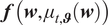 appearing in (2.12) matches the one of
$ \boldsymbol{R}\left(\boldsymbol{w}\right) $
 . This aspect and the proposed CNN are further discussed in Appendix D.
4. Results
The routines are first (§ 4.1) validated on the NASA 2D Wall-Mounted Hump for data assimilation of the
$ \beta $
 parameter (using both explicit and implicit strategies). We then consider a more ambitious configuration and progressively move toward the development of an algebraic turbulence model based on a CNN:
-
• First (§ 4.2), we verify that the BROADCAST code, combined with the baseline SA model, yields consistent results for the standard VKI LS-59 turbine blade cascade.
-
• Then (§ 4.3), we demonstrate that, given the SA solution for the VKI LS-59 case, $ {\boldsymbol{w}}^{SA}=\left[\rho, \rho \boldsymbol{U},\rho E\right] $
, we are able to satisfactorily reconstruct the SA eddy viscosity field
$ {\mu}_t^{SA} $
using the explicit residual minimization strategy by tuning
$ \boldsymbol{\alpha} ={\mu}_t $
. -
• In § 4.4, we first introduce a custom dataset of flow fields obtained with the SA model by varying both flow and geometric parameters. We then construct a CNN-based algebraic turbulence model $ {\mu}_{t,\boldsymbol{\vartheta}}\left(\boldsymbol{w}\right) $
that reproduces the SA eddy viscosity
$ {\mu}_t^{SA} $
over this dataset. To this end, the CNN weights
$ \boldsymbol{\vartheta} $
are optimized using the explicit strategy by minimizing the residual of a corrected model on the custom dataset.



Building an algebraic turbulence model capable of reproducing the results of a one-equation SA model is an extremely challenging task, even when using a CNN-based formulation (here with a limited kernel width). It is worth recalling that classical algebraic turbulence models, such as the model by Baldwin and Lomax (Reference Baldwin and Lomax1978), are generally well suited for attached turbulent boundary layers, but perform poorly in separated flows and in wake regions behind profiles, where the turbulent viscosity is significantly mispredicted. In such models, nonlocality is only partially accounted for through the distance to the closest wall; however, this does not capture streamwise nonlocal effects, which are particularly important in wake regions. This limitation notably motivated the introduction of transport-equation-based models, in which streamwise nonlocality is represented through the advection of turbulence variables. In the present approach, the CNN-based algebraic eddy viscosity model can be regarded as strongly local, since the distance to the closest wall is not included and the kernel width of the CNN is limited to that of the spatial scheme, that is, a few grid cells in each spatial direction (see § D for more details). As a result, the CNN learns local features based on the resolved state
$ \boldsymbol{w}=\left[\rho, \rho \boldsymbol{U},\rho E\right] $
 (and its derivatives) to predict the eddy viscosity
$ {\mu}_t $
 .
In the future, learning a CNN-based
$ \beta $
 turbulence production correction term from high-fidelity Large Eddy Simulations (LES) data appears to be a promising direction, as it naturally captures streamwise nonlocality while identifying local features. Increasing the kernel width provides additional flexibility but may violate the stencil locality of the numerical scheme, introducing extra couplings and modifying the sparsity structure of the associated operators.
4.1. 2D NASA Wall-Mounted Hump separated flow
The first case selected for the application of the framework is NASA’s 2D Wall-Mounted Hump (WH) (no plenum), shown in Figure 3. This case is characterized by a separation of the flow from the body with subsequent reattachment and boundary-layer recovery.
Outline of the geometry of the 2D NASA Wall-Mounted Hump with the corresponding boundary conditions.

It is a well-established benchmark configuration developed at NASA Langley Research Center for the validation of turbulence models in separated flows. It is widely used within the CFD community because it combines a relatively simple two-dimensional geometry with complex physical phenomena, including adverse pressure gradients, boundary-layer separation, recirculation, and reattachment. The case was designed to provide high-quality reference data, such as LES, against which RANS and hybrid turbulence models can be systematically assessed.
The geometry, as depicted in Figure 3, consists of a two-dimensional channel-like domain in which a smooth hump is mounted on the lower wall. Upstream of the hump, the lower wall is flat, allowing a turbulent boundary layer to develop under nearly equilibrium conditions. As the flow approaches and passes over the hump crest, it experiences a strong adverse pressure gradient that leads to boundary-layer separation downstream of the crest. This separation produces a recirculation bubble whose size and reattachment location are highly sensitive to turbulence modeling assumptions. Further downstream, the flow reattaches and gradually recovers toward a redeveloping turbulent boundary layer.
The canonical operating conditions correspond to a low-speed subsonic flow with a freestream Mach number of approximately
$ M\approx 0.1 $
 and a Reynolds number on the order of
$ \mathit{\operatorname{Re}}\approx 9.36\times {10}^5 $
 , typically based on a reference length associated with the hump geometry. Under these conditions, compressibility effects remain weak. At the inlet, a turbulent boundary layer consistent with the experimental measurements must be prescribed. The lower wall, including the hump, is treated as a no-slip boundary. The outlet is generally modeled as a pressure outlet with a specified static pressure to ensure the correct overall mass flow.
The primary validation quantities for this case include the surface pressure coefficient
$ {C}_p $
 , the skin-friction coefficient
$ {C}_f $
 , and mean velocity profiles at selected streamwise stations. The skin-friction distribution is especially important because it clearly identifies the separation and reattachment points.
A distinctive feature of the distributed two-dimensional grids is the nonflat upper boundary, which exhibits a mild contour rather than being straight. Although the hump is physically located only on the lower wall, the shaped upper wall is intentionally introduced to account for wind-tunnel confinement and blockage effects present in the original experiments. In the experimental setup, the test section had finite height and side plates, which influenced the global pressure distribution within the tunnel. A purely two-dimensional simulation with a flat and distant upper boundary would not reproduce these confinement effects accurately, leading to discrepancies in the pressure gradient imposed on the boundary layer over the hump. Since the separation process is driven by the adverse pressure gradient, even small differences in the global pressure field can significantly alter the predicted separation and reattachment behavior. To avoid performing a fully three-dimensional simulation of the entire wind tunnel, the two-dimensional benchmark geometry incorporates a carefully contoured upper wall that effectively mimics the experimental blockage. In this sense, the upper-wall shape acts as a surrogate for three-dimensional tunnel effects, allowing a two-dimensional computation to reproduce more faithfully the pressure distribution and separated-flow characteristics observed in the experiments.
More information on the case and the physical parameters imposed to run the RANS simulation can be found in Jespersen et al. (Reference Jespersen, Pulliam and Childs2016) and Pederson (Reference Pederson2021). Note that this case is part of the ERCOFTAC Database (Classic Collection). It is listed as Case C.83: Wall-mounted two-dimensional hump with oscillatory zero-mass-flux jet or suction through a slot.
4.1.1. Data assimilation with
$ \beta $
: partial-state measurements and implicit layer

In this section, we use the corrected model presented in (3.6) and the implicit optimization framework described in equations (2.26)–(2.27). The forward implicit solution in the underlined box is obtained by iteratively solving (2.9) with a direct-LU method. The backward implicit solution of the adjoint system uses this same inversion technique. For the definition of the cost functional to optimize, we use as a reference solution the LES simulation run by Uzun and Malik (Reference Uzun and Malik2018). Here, we consider partial-state measurements based solely on the streamwise and wall-normal velocity to define

and the data assimilation process aims at reconstructing the full state
$ \boldsymbol{w}=\left[\rho, \rho \boldsymbol{U},\rho E,\rho \tilde{\nu}\right] $
 , that is, in particular, the density, the temperature, and the turbulence variable which are considered unknown.
In this benchmark test, the routine was initialized with
$ \beta $
 set to zero throughout the domain. The BROADCAST solver is launched on a mesh of
$ {n}_i\times {n}_j=408\times 108 $
 cells in the
$ x $
 and
$ y $
 directions, respectively (
$ n={n}_i{n}_j $
 ).
The optimization algorithm uses the Limited-memory Broyden–Fletcher–Goldfarb–Shanno (L-BFGS) optimizer (Tankaria et al., Reference Tankaria, Sugimoto and Yamashita2022). The stopping criterion is reached when the variation in the normalized loss function satisfies a specified tolerance threshold (
$ {10}^{-6} $
 ). Figure 4 shows the behavior of the normalized objective function.
Data assimilation with
$ \beta $
 on Wall-Mounted Hump case handled with implicit layer: behavior of the normalized cost-function
$ \mathcal{J}/{\mathcal{J}}_0 $
 for 50 optimizer iterations using the L-BFGS PyTorch optimizer. The procedure is halted once the variation in the loss function satisfies a specified tolerance threshold. Specifically, the norm of the loss function starts at
$ 3.245\times {10}^{-4} $
 , and at the end of the computation, the reached value is
$ 6.611\times {10}^{-5} $
 .

We denote by
$ \beta \left(\boldsymbol{x}\right)={\beta}^{opt}\left(\boldsymbol{x}\right) $
 the value of the optimized spatial parameter after the final iteration. It is then possible to study the error fields for the
$ U $
 and
$ V $
 components of the velocity. Figures 5 and 6 show the local errors on the discretized mesh for the baseline and the optimized models, respectively. It is important to note that not all of the domain is shown in the figures since the LES reference values were available only in the depicted region.
Data assimilation with
$ \beta $
 on Wall-Mounted Hump case handled with implicit layer: representation of the error fields for the velocities computed with the SA turbulence model (the baseline) with respect to the LES solutions, normalized by the reference freestream velocity
$ {U}_{\infty } $
 . It is not possible to show the whole computational domain depicted in Figure 3 since the LES solution is available only in the central region of the computational mesh. As the region of primary interest is the recirculation zone downstream of the hump, the figure shows the error profiles with a zoom on this area.

Figure 5. Long description
Two side-by-side contour plots labeled a and b. Both plots use x as the horizontal axis ranging from -2 to 1.5 and y as the vertical axis ranging from 0 to 0.8.
Panel a displays the error field for U velocity. The main plot shows a light blue field with a white hump at x equals 0. A black outline box zooms into the recirculation zone downstream of the hump, displayed as an inset in the top left. This inset shows a gradient of error values, with dark red indicating high positive error near the bottom surface at x equals 1, and light blue indicating negative error in the upper flow. A vertical color bar on the right ranges from -0.154 at the bottom (dark blue) to 0.240 at the top (dark red).
Panel b displays the error field for V velocity. The main plot is predominantly light yellow. The inset in the top left zooms into the same recirculation zone, showing a concentrated pocket of dark blue (negative error) immediately behind the hump and a pocket of orange (positive error) further downstream. A vertical color bar on the right ranges from -0.063 at the bottom (dark blue) to 0.057 at the top (dark red).
Data assimilation with
$ \beta $
 on Wall-Mounted Hump case handled with implicit layer: representation of the error fields for the velocities at the final iteration with respect to the LES solutions, normalized by the reference freestream velocity
$ {U}_{\infty } $
 . It is not possible to show the whole computational domain depicted in Figure 3 since the LES solution is available only in the central region of the computational mesh. The same scales as Figure 5 were kept to highlight the decrease in errors. We can see that the
$ \beta $
 parameter is not sufficiently flexible to accurately reproduce the high-fidelity data in the recirculation region. Franceschini et al. (Reference Franceschini, Sipp and Marquet2020) showed that this may be understood by the rigidity of the chosen control parameter
$ \beta $
 . As the region of primary interest is the recirculation zone downstream of the hump, the figure shows the error profiles with a zoom on this area.

Figure 6. Long description
A two-panel visualization of error fields normalized by U sub infinity. Both panels use x as the horizontal axis ranging from -2 to 1.5 and y as the vertical axis ranging from 0 to 0.85.
Panel a, on the left, displays the error field for U. The main plot shows a light blue field with a white hump shape. A black outline box zooms into the recirculation region downstream of the hump, shown in the lower right. The color scale on the right ranges from -0.154 in dark blue to 0.240 in dark red. Significant error concentrations are visible as yellow and orange streaks near the hump surface and in the wake.
Panel b, on the right, displays the error field for V. The main plot is predominantly light yellow. Like panel a, a black outline box zooms into the recirculation zone at the bottom right. The color scale ranges from -0.063 in dark blue to 0.057 in dark red. The error patterns are more localized around the separation point and the immediate lee side of the hump compared to the U component.
In both panels, the L E S solution is only available in the central region, leaving the outer edges of the mesh blank.
Moreover, the optimization behavior can be assessed by analyzing the final distribution of
$ {\beta}^{opt}\left(\boldsymbol{x}\right) $
 and its impact on the eddy viscosity. In particular, we can compare the eddy viscosity obtained for the baseline model
$ \beta \left(\boldsymbol{x}\right)=0 $
 with that resulting from
$ {\beta}^{opt}\left(\boldsymbol{x}\right) $
 . Figure 7 shows three quantities: the initial eddy viscosity computed with the SA turbulence model, the corresponding eddy viscosity
$ {\mu}_t $
 obtained using
$ {\beta}^{opt} $
 , and the optimized correction field
$ {\beta}^{opt}\left(\boldsymbol{x}\right) $
 .
Data assimilation with
$ \beta $
 on Wall-Mounted Hump case handled with implicit layer.

Figure 7. Long description
A multi-panel figure with three vertically stacked contour plots. Each plot shares an x-axis from negative 6 to 4 and a y-axis from 0 to 0.8. A white semi-circular hump is located on the bottom wall at x equals 0.5.
Panel a shows eddy viscosity mu sub t super S A. The flow is mostly dark blue, indicating low viscosity. A plume of light blue to red emerges behind the hump, peaking at a value of 0.001270. The plume expands horizontally toward the right.
Panel b shows corrected eddy viscosity mu sub t super o p t. The distribution is similar to panel a but with a higher peak intensity of 0.002225 immediately downstream of the hump, shown in deep red.
Panel c shows the optimal correction field beta super o p t. The background is a uniform light blue. A concentrated region of high values, reaching 1.355, is localized specifically at the separation point on the lee side of the hump. The color bar on the right ranges from negative 0.566 to 1.355.
In all panels, the region upstream of the hump remains at the baseline value, while the significant data changes occur in the wake region to the right of the hump.
We can see that the turbulent viscosity computed with the optimized value of
$ \beta $
 has been increased in the recirculation bubble. These results demonstrate the potential of the approach and help identify areas for further refinement and optimization. One can also compare different models in terms of the
$ {C}_f $
 skin-friction coefficient and the
$ {C}_p $
 pressure coefficient. Figure 8 shows that the obtained results are closer to the LES values than those of the baseline SA turbulence model, thereby confirming that the optimization has yielded more accurate predictions.
Data assimilation with
$ \beta $
 on Wall-Mounted Hump case handled with implicit layer: comparison between wall-quantities computed from LES data Uzun and Malik, (Reference Uzun and Malik2018), RANS using the baseline SA model, and the corrected RANS model using the optimized
$ \beta $
 .

Figure 8. Long description
The image contains two panels labeled a and b. Both share a horizontal x-axis ranging from negative 0.50 to 1.50.
Panel a, labeled C sub p, shows the pressure coefficient on the vertical axis from negative 0.8 to 0.4.
- The L E S data (red squares) and D A-beta (black dashed line) are nearly identical, showing a sharp peak at x equals 0, a deep trough at x equals 0.6, and a recovery toward 0.
- The R A N S-S A model (cyan dashed line) deviates significantly during the recovery phase after x equals 0.75, underestimating the pressure coefficient compared to the other two.
Panel b, labeled C sub f, shows the skin friction coefficient on the vertical axis from negative 0.002 to 0.008.
- The L E S data shows a dip at x equals 0, a plateau between 0.25 and 0.6, and a sharp drop to negative values at x equals 0.7 before recovering.
- The R A N S-S A model overestimates the plateau significantly, reaching 0.007.
- The D A-beta model follows the L E S trend much more closely than the baseline R A N S, though it slightly underestimates the plateau height and shows a deeper trough at x equals 0.9 before recovery.
It is important to note that, for this study, at every iteration performed by the optimizer, a FP problem must be solved using a Newton method, after which another linear system must be inverted to compute the adjoint solution, as detailed in Section 2.2.2. Each iteration using the BROADCAST solver takes approximately one minute, depending on the hardware used, and benefits from multiprocessing to construct the sparse Jacobian matrices.
4.1.2. Data assimilation with
$ \beta $
: full-state measurements and explicit layer

In order to fully validate the developed framework, the explicit residual minimization strategy is applied to this same case. As mentioned above, such a strategy requires full-state information
$ {\boldsymbol{w}}_m $
 . We still consider the corrected model presented in (3.6), but we now apply the explicit optimization framework described in equations (2.19)–(2.20). The full-state
$ {\boldsymbol{w}}_m $
 is taken as the one obtained in the last section for the optimized value of
$ \beta $
 . The optimization algorithm is initialized with
$ \beta =0 $
 in the whole domain. Results are obtained using the Stochastic Gradient Descent (SGD) PyTorch optimizer, a tolerance threshold of
$ {10}^{-6} $
 being fixed for the variation in the normalized loss function.
This strategy is considerably faster than the implicit one, since instead of performing several Newton iterations, only a single evaluation of a Fortran function is needed. Figure 9 shows the behavior of the normalized objective function.
Data assimilation with
$ \beta $
 on Wall-Mounted Hump case handled with explicit layer: behavior of the normalized cost-function
$ \mathcal{J}/{\mathcal{J}}_0 $
 consisting here in the residual of the corrected RANS system for 2000 optimizer iterations using the SGD PyTorch optimizer. In this case, the proposed optimization procedure consistently reduces this residual by several orders of magnitude, reflecting a drastically improved consistency between the data and the corrected model.

The final values of
$ \beta $
 are shown in Figure 10.
Data assimilation with
$ \beta $
 on Wall-Mounted Hump case handled with explicit layer:
$ {\beta}^{opt} $
 obtained by minimizing the residual of RANS equations. It is possible to see that it is practically exact with respect to the results shown in Figure 7.

Figure 10. Long description
A 2 D contour plot displays data assimilation results on a wall-mounted hump. The horizontal x-axis ranges from negative 6 to positive 3, and the vertical y-axis ranges from 0 to 0.8. A white semi-circular hump is positioned on the bottom boundary between x equals 0 and x equals 1.
* The majority of the field is a uniform light blue, corresponding to a value near 0.010 on the color scale.
* A thin, light-colored layer extends along the bottom wall from x equals negative 5 toward the hump.
* Immediately downstream of the hump, centered near x equals 1 and y equals 0.1, is a concentrated elliptical region of high values. This region transitions from light blue to yellow, orange, and a dark red core, indicating values reaching up to 1.355.
* A vertical color bar on the right provides the scale for the beta super opt values, ranging from negative 0.566 at the bottom in dark blue to 1.355 at the top in dark red, with increments of approximately 0.19.
While the previous approach required solving many linear systems, this one only requires repeated calls to explicit functions of the CFD Fortran code compiled for Python. Therefore, the optimization using this strategy is much faster, performing thousands of iterations within minutes; however, it requires the full-state field.
4.2. Transonic flow through the VKI LS-59 turbine blade cascade: Validation of BROADCAST
We also consider a transonic flow passing between the blades of the VKI LS-59 turbine cascade (Hercus and Cinnella, Reference Hercus and Cinnella2011). The LS-59 geometry is a well-studied linear turbine blade cascade used both in experiments and numerical simulations to analyze aerodynamic losses, boundary-layer behavior, shock-boundary layer interactions, wake turbulence, and transition phenomena (Cinnella and Content, Reference Cinnella and Content2016; Jagodzińska et al., Reference Jagodzińska, Olszański, Gumowski and Kubacki2024; Gloerfelt and Cinnella, Reference Gloerfelt and Cinnella2025). For this case, either a C-mesh or an H-mesh is commonly used in the literature. These mesh types allow for proper discretization of the boundary layer around the airfoil.
The key aerodynamic phenomena to be addressed include the following:
-
• Shock-wave formation on the suction side when the flow becomes locally supersonic, and the associated interaction with the boundary layer, possibly leading to separation or shock-boundary layer interaction.
-
• Wake development downstream of the trailing edge, including turbulence intensity, wake spreading, and mixing losses. These wake effects influence the overall cascade loss and are sensitive to both Mach number and incoming turbulence.
-
• Influence of varying the outlet isentropic Mach number (subsonic vs. transonic) on the flow features above (shock strength, separation, wake behavior) and on the losses.
A mesh is generated to run a RANS simulation on this case. The BROADCAST solver requires structured meshes, as mentioned earlier; therefore, a single-block structured mesh of the inter-blade space is constructed, as shown in Figure 11. The boundary conditions are set as in the transonic case studied in Jagodzińska et al. (Reference Jagodzińska, Olszański, Gumowski and Kubacki2024), as depicted in Figure 11.
Representation of the outline of the VKI LS-59 structured mesh with the boundary conditions imposed in the CFD solver.

Figure 11. Long description
The diagram illustrates a computational fluid dynamics domain for a turbine blade passage.
* At the far left, a vertical solid line represents the inlet, labeled Fixed inflow with angle of attack alpha.
* Moving right, the domain is bounded by horizontal dash-dot lines labeled Periodic conditions 1 at the top and bottom.
* In the center, the airfoil surfaces are shown. The upper curved boundary is red and labeled Adiabatic solid wall Pressure side. The lower curved boundary is blue and labeled Adiabatic solid wall Suction side.
* Following the airfoil, the domain extends downward and to the right, bounded by dashed lines labeled Periodic conditions 2 at the top and bottom.
* At the far right, a vertical solid line represents the outlet, labeled Static pressure Static mach Dirichlet.
The following parameters were fixed: (i) mesh sizes and geometry:
$ {n}_i=300 $
 ,
$ {n}_j=120 $
 (
$ n={n}_i{n}_j $
 ), geometry from DOE, (ii) scheme: FE-MUSCL of order 7, (iii) turbulence model: SA, (iv) physical parameters:
$ {Mach}_{in}=0.275 $
 ,
$ {Mach}_{out} $
 from DOE,
$ \alpha $
 (angle of attack) from DOE,
$ {\mathit{\operatorname{Re}}}_{in}=2.68\times {10}^5 $
 ,
$ {\mathit{\operatorname{Re}}}_{out}=6.8\times {10}^5 $
 ,
$ {T}_{ext}=300K $
 ,
$ {P}_{ext}=1.01\times {10}^5 Pa $
 .
By then solving the RANS equations using the relaxation method (see § 2.1.2), it is possible to compare the results with reference or experimental data. To this end, the isentropic Mach number is computed and compared with the values reported in Jagodzińska et al. (Reference Jagodzińska, Olszański, Gumowski and Kubacki2024). The results are shown in Figure 12.
Solution of baseline SA model on VKI LS-59 case with Newton-based relaxation method: isentropic Mach Number at the wall computed with the BROADCAST solver with respect to experimental results extracted from Jagodzińska et al. (Reference Jagodzińska, Olszański, Gumowski and Kubacki2024).

Figure 12. Long description
The x-axis is labeled x forward slash c and ranges from 0.0 to 1.0. The y-axis is labeled M sub i s and ranges from 0.0 to 1.2. A legend in the top-left identifies a solid light red line as C F D and blue circular markers as Experiment.
Data follows two distinct branches forming a loop.
On the upper branch, the Experiment markers show a steady increase from M sub i s 0.3 at x forward slash c 0.0 to a peak of approximately 1.15 near x forward slash c 0.85. The C F D line closely follows this trend but exhibits a sharp oscillation or peak reaching 1.2 at x forward slash c 0.6 before returning to align with the experimental data. At the trailing edge near x forward slash c 0.95, the C F D line shows a vertical fluctuation before ending at 1.0.
On the lower branch, the data starts with a sharp dip in the C F D line near the origin, reaching almost 0.0, while experimental points begin at 0.3. Both datasets then converge, following a gradual curve that rises from M sub i s 0.2 at x forward slash c 0.2 to M sub i s 0.5 at x forward slash c 0.8. The C F D line and Experiment markers show high agreement along this lower trajectory.
4.3. Transonic flow through the VKI LS-59 turbine blade cascade: Data assimilation with
$ {\mu}_t $
with full-state measurements and explicit layer

We use the corrected model presented in (3.4) and the explicit optimization framework described in equations (2.19)–(2.20). The considered correction parameter is the eddy viscosity:

As previously explained, if the full velocity field is available, it is in principle possible to use the residual minimization technique to predict turbulent parameters of the flow. In the present case, given the full state, can we correctly predict the eddy viscosity? To check this, a trainable parameter tensor of the size of the mesh is initialized with a constant value throughout the domain and provided as
$ {\mu}_t $
 in the routine. The loss function is composed of two terms: first, the norm of the full residual (laminar baseline model plus turbulent forcing) with the state
$ {\boldsymbol{w}}_m $
 corresponding to the solution computed in the previous section (see Figure 12); second, a regularization term defined as
$ \gamma \parallel {\mu}_t{\parallel}_M^2 $
 , where
$ \gamma >0 $
 , to minimize the values of
$ {\mu}_t $
 if not needed (the initial condition starts from a nonzero positive
$ {\mu}_t $
 value and should tend to zero in the free-stream for instance).
By running the routine for 2000 optimizer iterations using SGD, both the behavior of the loss function and the final parameter field demonstrate the capabilities of this strategy. Figure 13 shows the evolution of the normalized residual norm (fig. a), the final
$ {\mu}_t $
 field (fig. b), and the pointwise absolute error of this solution w.r.t to the SA one, normalized by the maximal value of the SA solution (fig. c).
Data assimilation with
$ {\mu}_t $
 on VKI LS-59 case handled with explicit layer: results of the residual minimization strategy on the VKI LS-59 case with respect to SA results.

Figure 13. Long description
The figure consists of three panels labeled a, b, and c.
Panel a is a line graph at the top. The x-axis is labeled Optimizer iterations ranging from 0 to 2000. The y-axis is a logarithmic scale labeled J over J sub 0 ranging from 10 super 0 to 10 super minus 3. The blue line shows a sharp initial drop from 1 to 0.02 within the first 100 iterations, followed by a noisy but steady linear decrease on the log scale, reaching approximately 2 times 10 super minus 4 by iteration 2000.
Panel b is a contour plot on the bottom-left showing predicted eddy viscosity. The x and y axes represent spatial coordinates. The plot shows a turbine blade cascade with flow moving from left to right. High values, indicated by red and orange diagonal bands, are concentrated in the wake region behind the blades. The color scale on the right ranges from 0.0000000 in dark blue to 0.0004439 in dark red.
Panel c is a contour plot on the bottom-right showing pointwise absolute error percentage relative to the S A solution. The geometry is identical to panel b. Most of the flow field is dark blue, indicating near-zero error. Small streaks of light blue and yellow, representing errors between 1.60 and 4.80 percent, are visible in the far-field wake. The color scale on the right ranges from 0.00 in dark blue to 7.99 in dark red.
We can see that, for this case, the optimization framework accurately recovers the eddy viscosity. Since the state variables used are obtained from the SA model, the reconstructed
$ {\mu}_t $
 exhibits the characteristic features of this turbulence model. In particular, the retrieved
$ {\mu}_t $
 distribution correctly captures the decay within the viscous sublayers near the walls, as well as the destruction in the outer regions of the boundary layers. In the free-stream, the eddy viscosity is advected downstream without destruction, a characteristic behavior of the SA model. The largest relative errors (
$ >7\% $
 ) are localized in the wake region downstream of the blade, where thin convective structures and strong eddy viscosity gradients increase the sensitivity of the prediction. In these regions, small local discrepancies between the two fields may lead to amplified pointwise relative errors due to the sharp spatial variations of the solution. Nevertheless, the overall distribution and magnitude of the eddy viscosity field remain well reproduced.
4.4. Turbine flow modeling with a CNN for
$ {\mu}_t\left(\boldsymbol{w}\right) $

As outlined previously, our objective is to augment RANS simulations with data-driven corrections. To this end, a representative dataset of simulations is required for training the proposed model, with the VKI LS-59 cascade selected as the baseline configuration. In this section, we first present the dataset (§ 4.4.1) and then use the explicit strategy to learn a predictive model for the eddy viscosity based on full-state fields
$ {\boldsymbol{w}}_m $
 from the dataset (§ 4.4.2).
4.4.1. Generation of the dataset
When using an ML model, special care must be taken, especially if spatial convolutions are required. To balance the requirements imposed by the solver, a single-block structured mesh discretizing the blade passage is considered. For all parameters, the topology and the number of cells in each direction are kept constant. The suction and pressure sides of the blade are split, positioning them in the upper and lower parts of the computational domain, respectively. This solution addresses the challenges of using ML models but requires particular attention during mesh generation to (i) correctly discretize the boundary layer, (ii) avoid overly stretched cells at the leading and trailing edges of the blade, and (iii) adapt the domain shape to better align the flow with the generalized computational coordinates. To achieve this, a custom elliptic mesh generator has been implemented. Specifically, by varying the control points used to define the camber line of the blade and the angle of rotation, many different meshes can be generated with the same tool.
To illustrate the effectiveness of the mesh generator, Figure 14 presents the collection of blade profiles generated, in comparison with the original blade geometry and its corresponding control points. These variations highlight the flexibility of the parametrization strategy in exploring a wide design space around the reference configuration. The original profile and control points, extracted from Hercus and Cinnella (Reference Hercus and Cinnella2011), are shown for reference.
Superposition of all generated blade geometries with the original blade profile and control points (from Hercus and Cinnella, Reference Hercus and Cinnella2011).

Figure 14. Long description
The graph uses an X-axis ranging from 0.0 to 1.0 and a Y-axis from 0.0 to 0.5.
* The Nominal geometry is represented by a thick black dashed line forming a curved airfoil shape. Its internal structure is marked by a thin black dashed line for the camber line and black circular control points.
* The Most different geometry is shown as a thick red dashed line that expands the upper surface of the airfoil significantly. It includes a red dashed line with star markers for its camber line and red star control points, one of which is positioned high above the others at approximately X = 0.1, Y = 0.54.
* Other geometries appear as a dense cyan cloud of thin lines filling the space between and around the nominal and extreme profiles, illustrating the range of generated blade variations.
* All geometries converge at two common points at the leading edge near 0,0 and the trailing edge near 1,0.
The resulting dataset, comprising all generated geometries and corresponding simulation data, has been made openly accessible to the research community and is available at Bucci et al. (Reference Bucci, Saverio and Casenave2025). This resource aims to foster reproducibility and further investigations in the field of turbo-machinery optimization and data-driven turbulence modeling. Moreover, this dataset, together with several others structured in the Plaid format, has been used to assess the performance of different surrogate models. A comprehensive analysis of these applications is provided in Casenave et al. (Reference Casenave, Roynard, Staber, Piat, Bucci, Akkari, Kabalan, Nguyen, Saverio, Perez, Kalaydjian, Fouché, Gonon, Najjar, Menier, Nastorg, Catalani and Rey2025).
To create the dataset, a Design of Experiments (DOE) was generated using the maximum projection algorithm (Joseph et al., Reference Joseph, Gul and Ba2015). Table 1 shows the intervals chosen for the parameters, and the remaining parameters were fixed as detailed in Section 4.2 (Further details can be found at Bucci et al., Reference Bucci, Saverio and Casenave2025.).
Parameters and ranges used to generate the DOE

Table 1. Long description
The table consists of three columns: Parameter, Minimal value, and Maximal value.
* Row 1: Distance of the 2 degree point from the 1 degree control point ranges from minus 0.15 to 0.15.
* Row 2: Angle of attack ranges from 10 degrees to 50 degrees.
* Row 3: Delta x of the 3 degree control point from the original geometry ranges from minus 0.2 to 0.2.
* Row 4: Delta y of the 3 degree control point from the original geometry ranges from minus 0.2 to 0.2.
* Row 5: Pitch (inter-blades distance) ranges from 0.68 to 1.1.
* Row 6: Mach number at outflow ranges from 0.75 to 0.98.
In Appendix B, the dataset is analyzed further, showing its completeness and sensitivity with respect to the parameters used in the DOE; see Table 1.
4.4.2. Closure with
$ {\mu}_t $
using a CNN and explicit layer

We still use the corrected model presented in (3.4) and the explicit optimization framework described in equations (2.19)–(2.20).
Optimization with respect to an eddy viscosity model depending on the state
$ \boldsymbol{w} $
 is now performed:

The model
$ {\mathcal{M}}_{\boldsymbol{\vartheta}} $
 can be any kind of NN. For this study, a CNN is selected since we are dealing with structured meshes. CNNs exploit spatial correlations through convolutional filters, making them particularly effective at capturing local flow features such as gradients, shear layers, and boundary-layer structures. Moreover, compared to fully connected or recurrent architectures, CNNs require fewer parameters for high-dimensional inputs, improving both training efficiency and generalization.
The dataset generated from BROADCAST simulations in the last section has been split into training (80%) and validation (20%) subsets. This division ensures that the model can be optimized effectively while monitoring its generalization performance on unseen data.
Different optimization algorithms available in PyTorch were tested; the L-BFGS optimizer was ultimately selected to produce the reported results, using a mini-batch size of 100. During training, the cost functional
$ \mathcal{J}/{\mathcal{J}}_0 $
 decreases by approximately two orders of magnitude, reaching
$ {\mathcal{J}}_f/{\mathcal{J}}_0=\left(4.75\pm 1.39\right)\times {10}^{-3} $
 over 10 independent runs (mean
$ \pm $
 standard deviation). The corresponding validation value is
$ {\mathcal{J}}_f^{\mathrm{val}}/{\mathcal{J}}_0=\left(6.35\pm 0.83\right)\times {10}^{-3} $
 , indicating limited sensitivity to the random initialization of the network weights and to the mini-batch training procedure. Although L-BFGS is classically formulated in a deterministic full-batch setting, mini-batch variants have also been investigated in the optimization literature (Berahas and Takáč, Reference Berahas and Takáč2019). Although these final values are of the same order of magnitude as those obtained in Fig. 13a, the latter corresponds to the direct optimization of
$ {\mu}_t $
 for a single configuration, for which nearly perfect convergence could be achieved. In the present case, the optimization is carried out over a diverse set of configurations so that the network parameters must provide a global compromise rather than an exact optimum for a single case.
Figure 15 provides a visualization of the model predictions for two randomly selected configurations (cases 676 and 679, whose simulation parameters are presented in Table 2) drawn from the validation set. For each configuration, two fields are shown to offer a thorough assessment of the model’s performance. The first field represents the predicted eddy viscosity distribution, denoted as
$ {\mu}_{t,\boldsymbol{\vartheta}}\left(\boldsymbol{w}\right) $
 , across the entire domain. The second field illustrates the absolute pointwise percentage error in the eddy viscosity with respect to the SA eddy viscosity obtained with the BROADCAST solver,
$ \mid {\mu}_{t,\boldsymbol{\vartheta}}\left(\boldsymbol{w}\right)\left(\boldsymbol{x}\right)-{\mu}_t^{SA}\left(\boldsymbol{x}\right)\mid /{\max}_{\boldsymbol{x}}{\mu}_t^{SA}\left(\boldsymbol{x}\right) $
 .
Closure with a CNN for
$ {\mu}_t $
 on custom dataset handled with explicit layer: eddy viscosity prediction on two cases extracted from the validation set.

Figure 15. Long description
A four-panel grid of contour plots labeled a through d. Each plot uses x and y axes to map spatial coordinates around three curved turbine blades.
Panel a, top-left, shows predicted eddy viscosity mu sub t comma theta for case 6 7 6. The flow enters from the left in solid blue and develops into diagonal bands of red and orange, indicating higher viscosity, as it passes between and behind the blades. The color bar ranges from 0.0000000 to 0.0005033.
Panel b, top-right, shows the error percentage for case 6 7 6 compared to the S A turbulence model. The field is predominantly blue, indicating low error, with small light blue and white patches near the blade trailing edges. The color bar ranges from 0.00 to 45.65.
Panel c, bottom-left, shows predicted eddy viscosity for case 6 7 9. Similar to panel a, it shows diagonal high-viscosity streaks in red and yellow trailing from the blades. The color bar ranges from 0.0000000 to 0.0004880.
Panel d, bottom-right, shows the error percentage for case 6 7 9. Like panel b, the majority of the flow field is dark blue, with localized error spikes in lighter blue near the blade surfaces. The color bar scale is identical to panel b, ranging from 0.00 to 45.65.
Simulation parameters for cases 676 and 679
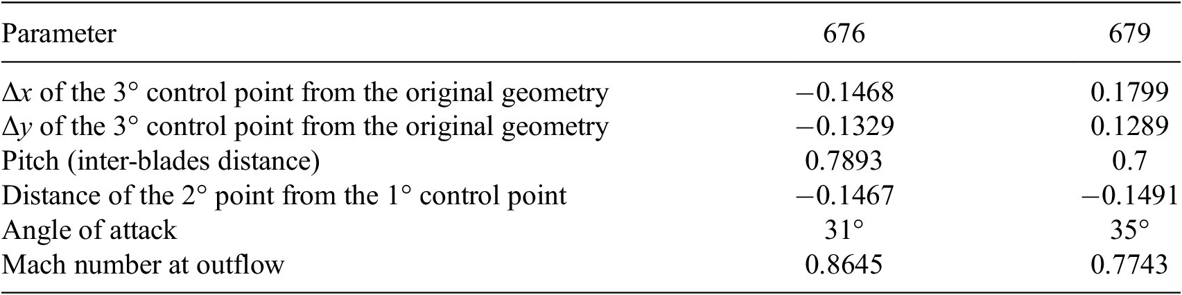
Table 2. Long description
The table consists of three columns: Parameter, 676, and 679.
* Delta x of the 3 degree control point from the original geometry: -0.1468 for case 676 and 0.1799 for case 679.
* Delta y of the 3 degree control point from the original geometry: -0.1329 for case 676 and 0.1289 for case 679.
* Pitch (inter-blades distance): 0.7893 for case 676 and 0.7 for case 679.
* Distance of the 2 degree point from the 1 degree control point: -0.1467 for case 676 and -0.1491 for case 679.
* Angle of attack: 31 degrees for case 676 and 35 degrees for case 679.
* Mach number at outflow: 0.8645 for case 676 and 0.7743 for case 679.
The results show that the CNN-based algebraic turbulence model, despite its locality constraint, is capable of accurately reconstructing the eddy viscosity in the wake of profiles. This can be attributed to the fact that the CNN does not rely on explicit quantities such as the distance to the closest wall, in contrast to classical algebraic turbulence models. Furthermore, the errors are small in the attached regions of the boundary layers, while they remain nonnegligible on the suction side of the profiles near the trailing edge, where flow separation occurs. This clearly indicates that a local algebraic turbulence model does not possess sufficient degrees of freedom to accommodate the full range of flow regimes, including attached boundary layers, separated boundary layers, and wake regions.
To further assess the robustness of the proposed framework, we consider an ensemble of models differing only by random initialization and stochastic optimization. The ensemble is constructed from the same 10 runs used in the training and validation loss analysis, allowing us to quantify prediction variability and estimate epistemic uncertainty.
For case 676, previously presented, we compute the ensemble mean and standard deviation of the predicted turbulent viscosity field. The ensemble mean, shown in Figure 16a, closely matches the previously reported prediction, demonstrating the consistency of the model across different training instances.
Closure with a CNN for
$ {\mu}_t $
 on custom dataset handled with explicit layer: ensemble statistics of the predicted turbulent viscosity field for case 676. The mean field highlights the robustness of the prediction, while the standard deviation identifies regions of higher variability across models.

Figure 16. Long description
A two-panel visualization of turbulent viscosity fields around three turbine blade profiles. Both panels use an x-axis ranging from 0.0 to 1.5 and a y-axis ranging from -2.0 to 1.5.
* Left Panel (a) Ensemble mean: Displays the average predicted mu sub t field. The flow enters from the left in a uniform dark blue region. As it passes the three white blade profiles, high-intensity red and orange streaks emerge from the trailing edges, indicating wake regions with high turbulent viscosity. The color scale on the right ranges from 0.0000033 at the bottom (dark blue) to 0.0004942 at the top (dark red).
* Right Panel (b) Ensemble standard deviation (percentage): Displays the variability across models. The regions surrounding the blades and the wake paths are light blue, while small pockets of darker blue and yellow appear near the blade surfaces and in the immediate wake. The color scale on the right ranges from 0.21 at the bottom (dark blue) to 27.09 at the top (dark red), representing the percentage of variability.
In contrast, the standard deviation, reported in Figure 16b, reveals localized regions of increased variability. Notably, these regions correspond to areas where larger prediction errors were observed in the previous analysis. This correlation between ensemble spread and prediction error suggests that the standard deviation can serve as a meaningful indicator of model uncertainty and reliability.
Overall, this analysis highlights the benefit of ensemble-based approaches for identifying regions of reduced confidence in the predictions, providing additional insight that is not accessible from a single model realization.
Several directions could be explored to further improve the proposed framework. These include the use of richer architectures (e.g., increased channel capacity or alternative field embeddings such as implicit neural representations), the incorporation of tags in the input fields to explicitly encode the boundary conditions information, and modifications of the loss function, for instance, through importance sampling based on velocity gradients or by adding a regularization term directly on the turbulent viscosity. Finally, much care must be taken to ensure that the trained model behaves robustly when embedded within a Newton solver, in particular, with respect to FP stability. These aspects will be addressed in future work.
5. Discussions and conclusions
The main objective of this work was to demonstrate the capability of the proposed framework to perform end-to-end optimization within a fully differentiable and physically consistent pipeline.
After introducing the optimization problem, the reference configurations, and the training dataset, the first two test cases show that both optimization strategies are fully operational. In particular, the explicit residual minimization and the implicit Newton-like solver correctly propagate gradients through the entire computational chain in a truly end-to-end fashion. This validates the correctness of the proposed formulation and its seamless integration within a differentiable programming environment.
The results further confirm the effectiveness of the proposed approach in predicting the eddy viscosity directly from the conservative flow variables. These findings highlight the potential of the framework as a reliable tool for data-assisted turbulence modeling and provide a solid basis for future developments aimed at improving accuracy, robustness, and scalability.
While demonstrated here for RANS turbulence modeling, the proposed framework is general and extends naturally to PDE-constrained systems with embedded closure models. It thus establishes a consistent and scalable paradigm for integrating trainable components within physics-based solvers via differentiable formulations and adjoint-based optimization.
The most natural extension of this work is the application of the implicit (Deep Equilibrium) strategy to the developed dataset, still targeting the prediction of the eddy viscosity in the Spalart–Allmaras turbulence model. Further extensions may include the adoption of more complex neural architectures, the treatment of different closure problems, and the investigation of transfer capabilities across distinct flow regimes. These directions will contribute to strengthening the synergy between numerical modeling and data-driven methodologies in computational physics.
Acknowledgments
We would like to thank Pedro Stefanin Volpiani for all the helpful discussions and advice during the development of this work.
Author contribution
Conceptualization: M.A.B., C.C., D.S.; software: L.S., G.F., C.C; validation: L.S., G.F.; methodology: L.S., M.A.B., C.C.; data curation: L.S., M.A.B., G.F.; data visualization: L.S.; writing original draft: L.S.; supervision: M.A.B., C.C., D.S. All authors approved the final submitted draft.
Data availability statement
The presented VKI dataset (Bucci et al., Reference Bucci, Saverio and Casenave2025), comprising all generated geometries and corresponding simulation data, has been made openly accessible to the research community and is available at https://doi.org/10.5281/zenodo.14840512. The open-source CFD solver BROADCAST (Poulain et al., Reference Poulain, Content, Sipp, Rigas and Garnier2023) is available on GitHub at https://github.com/onera/Broadcast. The LES data of the 2D NASA Wall-Mounted Hump can be accessed at https://turbmodels.larc.nasa.gov/Other_LES_Data/nasa_hump_uzun_2017.html.
Funding statement
This work was partially supported by the French National Research Agency under project ANR-22-FAI2-0002-01.
Competing interests
The authors declare none.
Ethical standards
The research meets all ethical guidelines, including adherence to the legal requirements of the study country.
A. PyTorch routines
All routines described in this work are implemented in Python, while the underlying CFD solver, including its numerical schemes, is implemented in Fortran and compiled (e.g., using Intel or gfortran compilers) as Python-callable libraries. These are interfaced with PyTorch via ctypes and wrapped using torch.autograd.Function. This hybrid approach combines the robustness of established numerical solvers with the flexibility and differentiability of modern ML frameworks.
This modular structure allows not only precise control over each component of the solver but also facilitates generalization to other PDE systems. This strategy, used for the boundary condition layer (BC) in Listing 1, can be replicated for other components of a numerical scheme, making the framework extensible and adaptable to a wide range of physics-informed learning tasks.
Listing 1: BC Autograd Function.
1 class BC(torch.autograd.Function):
2 @staticmethod
3 def forward(u):
4 return bc.f90(u)
5 @staticmethod
6 def backward(grad):
7 return bc_adj.f90(grad)
8 @staticmethod
9 def jvp(u_lin):
10 return bc_lin.f90(u_lin)
Once the individual computational blocks have been defined and wrapped as differentiable layers, they can be composed into a single torch.nn.Module that encapsulates the entire forward computation. When the backward pass is triggered—either during training or optimization—PyTorch automatically applies the chain rule across the composed operations. This ensures that the gradients of the loss function with respect to the trainable parameters are correctly propagated through each step of the numerical solver.
In the specific case of the RANS equations, the complete differentiable module is constructed by sequentially stacking the custom layers for boundary condition imposition (BC), flux computation (NS), and turbulence forcing (FORCE). The resulting torch.nn.Module, shown in Listing 2, acts as a differentiable surrogate for the physical solver and can be directly integrated into the learning loop.
Listing 2: RANS Module.
1 class RANS(nn.Module):
2 def _ _init_ _(self, params):
3 super()._ _init_ _()
4 self.BC_layer = BC()
5 self.NS_layer = NS()
6 self.F_layer = F()
7 self.parameters = params
8 def forward(self, u):
9 u_bc = self.BC_layer(u)
10 return self.NS_layer(u_bc) + self.F_layer(u_bc, self.parameters)
Finally, once an iterative solver is selected and the action of the Jacobian of the system can be evaluated (either explicitly or in a matrix-free manner), it becomes possible to define a custom torch.autograd.Function for the entire solution process. In this formulation, the system of governing equations is solved implicitly, and the backward method is overridden to compute gradients via the adjoint system, rather than backpropagating through each individual nonlinear iteration and its associated linear solves. This significantly reduces memory consumption and improves computational efficiency, as it avoids the need to store or differentiate through the full unrolled iteration path.
This concept is closely related to the philosophy behind Deep Equilibrium Models (DEQs) (Bai et al., Reference Bai, Kolter and Koltun2019), where FP equations are treated as implicit layers and differentiated through using the implicit function theorem. In the present work, this strategy is adopted to compute gradients consistently with the physics-based residual while maintaining full compatibility with the PyTorch optimization ecosystem. The implemented FP module is shown (in pseudo-code) in Listing 3.
Listing 3: Newton Solver Layer.
1 class FIXED_POINT(torch.autograd.Function):
2 @staticmethod
3 def forward(ctx, x, parameters, config_rans, config_FP):
4 x_sol, J = NEWTON_solver(x, parameters, config_rans, config_FP)
5 ctx.save_for_backward(x_sol, parameters)
6 ctx.JT = torch.transpose(J, 0, 1)
7 return x_sol
8 @staticmethod
9 def backward(ctx, grad_output):
10 saved = ctx.saved_tensors
11 x_sol, parameters = saved
12 JT = ctx.JT
13 lambda_ = ADJOINT_solver(JT, grad_output)
14 f = F(x_sol, parameters)
15 grads_params = torch.autograd.grad(outputs=f, inputs=parameters, grad_outputs=lambda_)
16 return None, grads_params, None, None
B. Completeness and sensitivity of the dataset
The DOE procedure described in Section 4.4.1 generated a total of 1500 distinct parameter sets. Each of these sets was used to run a numerical simulation, resulting in 840 successfully converged cases, having defined a tolerance for the value of the RANS residual. To assess the representativeness and coverage of the sampled parameter space, a univariate statistical analysis was performed. Specifically, a histogram was constructed for each parameter, illustrating the distribution of the converged cases within the original design space, as shown in Figure B1 for every parameter.
Histograms of the input parameters for the converged simulations. Despite the removal of some cases due to lack of convergence, the retained simulations remain well distributed across the prescribed parameter ranges, ensuring a representative coverage of the design space.

Figure B1. Long description
The figure consists of six blue histograms arranged in a two-by-three grid. Each plot has Frequency on the y-axis and Value on the x-axis.
* Panel a, Converged param s: Values range from 0.7 to 1.1. The distribution is relatively uniform with a slight peak around 0.75 and a gradual decline toward 1.1.
* Panel b, Converged param distance P 1-P 2: Values range from -0.15 to 0.15. The frequency is highest between -0.15 and -0.10, showing a slight downward trend as values increase toward 0.15.
* Panel c, Converged param position x-P 3: Values range from -0.20 to 0.20. The distribution is highly uniform across the entire range with minor fluctuations between frequencies of 20 and 35.
* Panel d, Converged param position y-P 3: Values range from -0.20 to 0.20. Similar to panel c, it shows a broad, uniform distribution with a slight peak near 0.05.
* Panel e, Converged param alpha: Values range from 10 to 50. The distribution is stable across the range, with the highest frequency occurring at the lower bound of 10.
* Panel f, Converged param mach outflow: Values range from 0.75 to 1.00. The frequency is higher and more stable between 0.75 and 0.85, followed by a more volatile distribution with a notable dip around 0.90 before rising again at 0.98.
To further investigate the sensitivity of the output variables with respect to the input parameters, a variance-based global sensitivity analysis was conducted using Sobol indices. To this end, a dimensionality reduction was applied to both the geometrical data and the physical simulation outputs using principal component analysis (PCA) (Pearson, Reference Pearson1901).
For the geometrical data, consisting of the
$ x $
 and
$ y $
 coordinates of the computational mesh nodes, a PCA was performed to identify the dominant deformation modes. By retaining 99.9% of the total variance, only four principal components were required. This result confirms that the selected geometrical design parameters are sufficient to span the space of observed shape variations.
Similarly, a PCA was applied to the set of conservative state variables (e.g.,
$ \rho $
 ,
$ \rho u $
 ,
$ \rho v $
 ,
$ \rho E $
 ,
$ {\mu}_t $
 ) at convergence. In this case, 50 principal components were necessary to capture the same amount of variance, reflecting the higher complexity of the solution fields.
Next, a Gaussian Process (GP) regression model (Casenave et al., Reference Casenave, Staber and Roynard2023) was trained to approximate the mapping from the reduced input space (comprising the four geometrical modes and two physical parameters) to the reduced output space defined by the 50 conservative modes. This nonintrusive surrogate model enables efficient evaluation of the model response across the input domain.
Finally, zero-order and first-order Sobol indices were computed using the trained GP model, allowing for a quantitative assessment of the influence of each input parameter on the variance of the output. These indices provide insight into both the individual effects and the interactions among parameters. Figure B2 shows the Sobol indices for each parameter for the first four and last four modes.
Sobol sensitivity indices for selected principal modes of the conservative variables. In red the
$ {0}^{th} $
 order indices and in green the
$ {1}^{st} $
 order. The first four modes capture dominant flow features, while subsequent modes highlight the contribution of input parameters to higher-order variations.

Figure B2. Long description
A multi-panel figure containing eight scatter plots arranged in a two-by-four grid, labeled 1, 2, 3, 4, 47, 48, 49, and 50. Each plot shares a common X-axis labeled Input variables ranging from 0 to 5 and a Y-axis labeled First order Sobol ranging from 0.0 to 1.0.
* Panel 1: Green indices are high (0.4 to 0.6) while red indices remain near zero.
* Panel 2: Both red and green indices spike sharply at input variable 4, reaching approximately 0.9 and 1.0 respectively.
* Panel 3: Green indices peak at input variable 1 (0.7) and red indices peak at variable 1 (0.6).
* Panel 4: Green indices peak at input variable 3.5 (0.5) and red indices peak at variable 3 (0.4).
* Panels 47 through 50: These higher-order modes show a more distributed pattern where green indices fluctuate between 0.2 and 0.7, and red indices fluctuate between 0.0 and 0.2.
In all plots, green markers represent 1st order indices and red markers represent 0th order indices, both accompanied by vertical error bars indicating uncertainty ranges.
C. Computing the gradients for the backward operation in PyTorch
Section 2.2.2 details how the gradients must be computed to correctly implement the backward operation. In practice, what is done in the code is a change of variable
$ \tilde{\boldsymbol{\vartheta}}=\boldsymbol{N}\boldsymbol{\vartheta } $
 at the definition of the problem:

We can then directly compute the partial derivative of the Lagrangian with respect to
$ \tilde{\boldsymbol{\vartheta}} $
 as follows:

then, since
$ \boldsymbol{N} $
 is a symmetric matrix, (Since the mass matrix
$ \boldsymbol{M} $
 is diagonal, the associated Cholesky factor
$ \boldsymbol{N}=\sqrt{\boldsymbol{M}} $
 is diagonal and thus symmetric.) the differential of the loss function is computed as follows:

which is precisely as computed in (2.25), but with respect to the new variable
$ \tilde{\boldsymbol{\vartheta}} $
 (see also (2.18)).
Therefore, if done correctly, PyTorch can compute the gradients automatically. This is achieved by first applying the change of variable in a torch.nn.Module and then applying the torch.autograd.Function; in this case, the gradients of these operations are concatenated correctly by the compiler, without any further correction by the user. This operation can be observed in Listing 5. It is nonetheless essential to define the loss function correctly, as shown in Listing 4:
Listing 4: Loss definition in Python and call to the backward mode.
1 vol = torch.from_numpy(self.config_deq["vol"])
2 loss = 0.5 * torch.sum(vol.unsqueeze(-1)*(out-reference)**2)
3
4 # vol is a tensor of shape (im, jm),
5 # while out and reference have shape (im, jm, em)
6
7 loss.backward()
Listing 5: Change of variable in the forward pass of the outer torch.nn.Module.
1 class RANSLayer(nn.Module):
2 def _ _init_ _(self, theta_tilde_init, config_rans, config_FP):
3 super().__init__()
4 self.theta_tilde = theta_tilde_init # parameters
5 self.config_rans = config_rans
6 self.config_FP = config_FP
7
8 def forward(self, x):
9 Nm1 = torch.from_numpy(self.config_FP["vol"])**(-0.5)
10 theta = Nm1 * self.theta_tilde
11 return FIXED_POINT.apply(x, theta, self.config_rans, self.config_FP)
D. Architecture of the developed Convolutional Neural Network
The NN employed in this work (see § 4.4.2) is designed to approximate the relationship between the mean-flow conservative variables and the turbulent eddy viscosity field,
$ {\mu}_t\left(\boldsymbol{w}\right) $
 . The input is given by the volumes of the discretized mesh and the discrete flow field
$ \boldsymbol{w} $
 , including ghost cells (see § 3.4), while the output is defined only on the physical cells, consistently with the definition of the closure term.
The architecture, as shown in Table D1, combines one-dimensional convolutional layers with fully connected (linear) layers and nonlinear activation functions. The convolutional part is used to extract local flow features, while the fully connected layers map these features to the final correction. The choice of one-dimensional convolutions is guided by the structured nature of the mesh and ensures invariance with respect to rotations aligned with the grid directions, as the same convolutional filter is applied along each coordinate direction (as shown in Figure D1). Furthermore, it avoids the need to define ghost-cell values at corner locations, where boundary conditions from different directions may overlap, thus preventing potential inconsistencies in the treatment of boundary regions.
A key aspect of the design concerns the spatial support of the convolutional kernels. In particular, the kernel size is kept smaller than the stencil width of the underlying numerical scheme. This ensures that the dependence of
$ {\mu}_t\left(\boldsymbol{w}\right) $
 on the state remains local and does not introduce additional couplings beyond those already present in the discretization. As a result, the sparsity pattern of the Jacobian
$ {\partial}_{\boldsymbol{w}}\left(\boldsymbol{R}+{\boldsymbol{f}}_{\boldsymbol{\vartheta}}\right) $
 is preserved, which is crucial for both the consistency and the efficiency of the solver, especially when adjoint-based gradient computations are involved. This aspect becomes even more relevant when sparse linear solvers are used (see § 3.4).
From an implementation standpoint, care is taken to ensure consistency between input and output domains. Ghost cells are included in the input to provide boundary information to the convolutions, but are excluded from the output, so that the predicted eddy viscosity is defined only on physically meaningful cells. This is also done to avoid introducing artificial boundary effects and to maintain compatibility with the numerical solver.
Architecture of the CNN used in this work

Table D1. Long description
The table consists of three columns: Layer, Type, and Specification. It details four sequential layers:
* Layer 1: Type is Conv 1 D with a Specification of Kernel size = 5.
* Layer 2: Type is Activation with a Specification of Si L U.
* Layer 3: Type is Conv 1 D with a Specification of Kernel size = 5.
* Layer 4: Type is M L P with a Specification of Linear layers with Si L U activation.
Schematic illustration of the convolutional kernel. The light blue cells denote the physical domain and the white cells the ghost cells. The convolutional kernels (yellow, red, and green) are chosen smaller than the stencil of the numerical scheme, ensuring locality and preventing the introduction of additional couplings. This preserves the sparsity pattern of the Jacobian matrix. Moreover, the kernels applied along the different directions share the same weights (indicated by identical colors), enforcing rotational invariance with respect to the grid. The contributions from the different convolutional directions are then combined in the physical domain.

Figure D1. Long description
The diagram consists of two parallel processing paths that converge at the bottom.
Top-Left Path:
* An input grid shows a light blue physical domain surrounded by white ghost cells.
* Three horizontal colored kernels are shown: a yellow kernel labeled filter at the top left, a red kernel in the center, and a green kernel at the bottom right.
* Dashed arrows point down to a second grid labeled Conv 1 d with a right-pointing arrow.
* In this second grid, the kernels have been reduced to single colored cells (yellow, red, and green) within the physical domain.
Top-Right Path:
* A similar input grid is shown, but with vertical colored kernels: a yellow vertical bar on the left, a red vertical bar in the center, and a green vertical bar on the right.
* Dashed arrows point down to a second grid labeled Conv 1 d with a down-pointing arrow.
* Like the left path, these kernels are reduced to single colored cells in the physical domain.
Convergence:
* Solid black arrows from both paths point toward a central circle containing the summation symbol Sigma.
* A final arrow points from the summation symbol to a single output grid at the bottom.
* This output grid contains the combined contributions, showing the yellow, red, and green cells in their respective positions within the light blue physical domain.
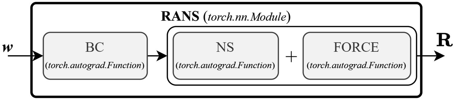
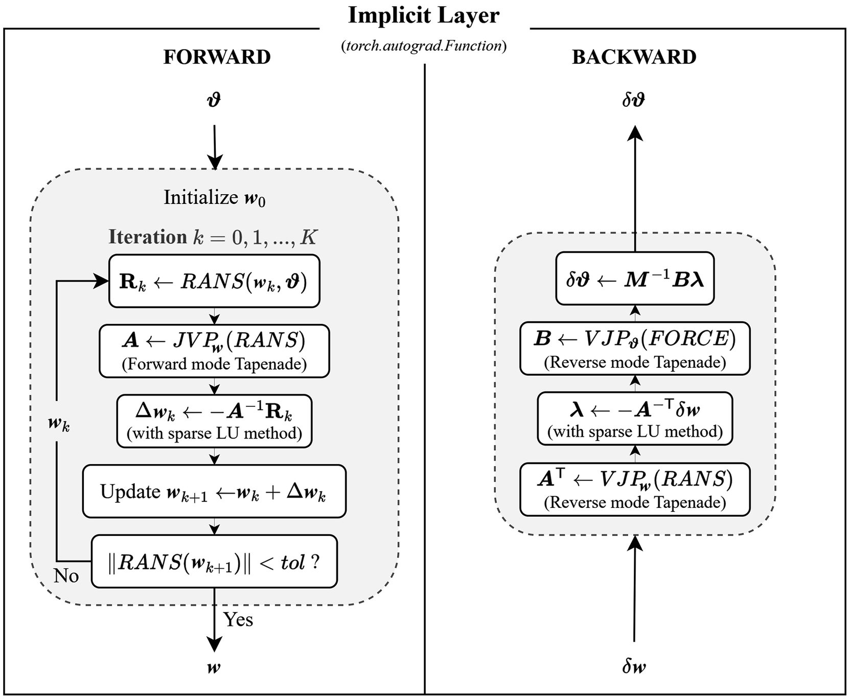
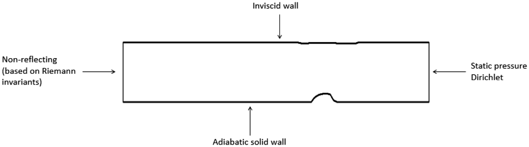
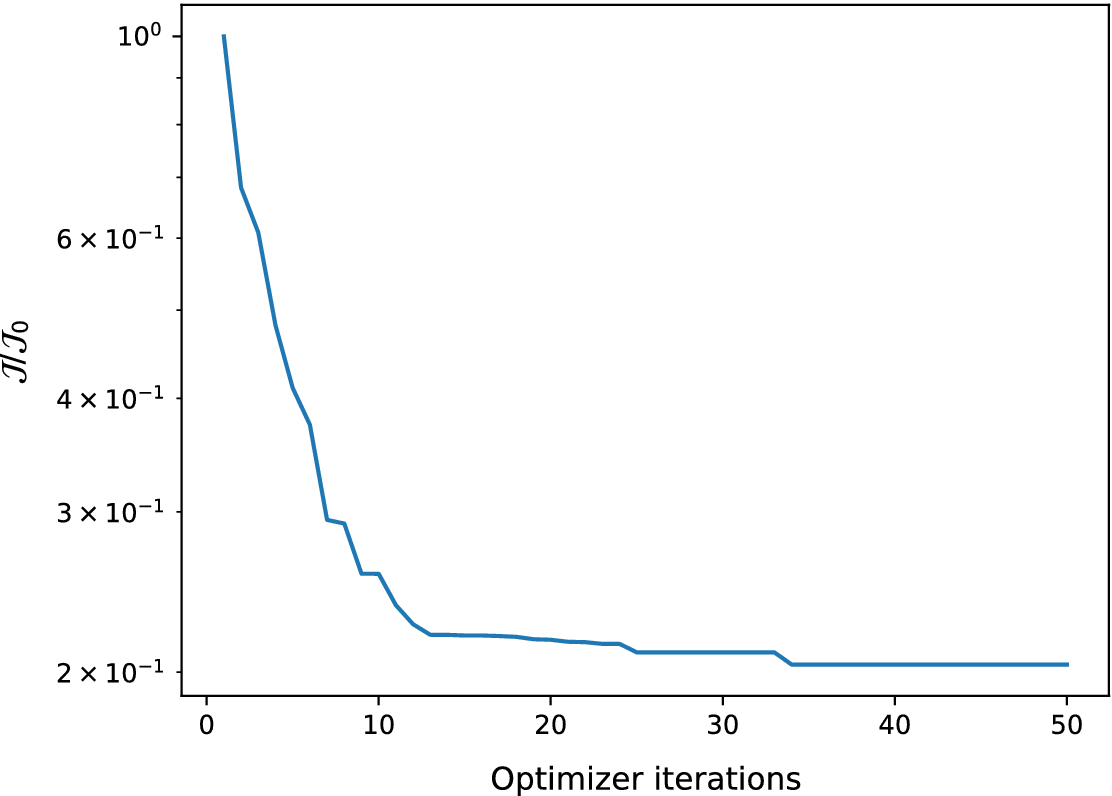


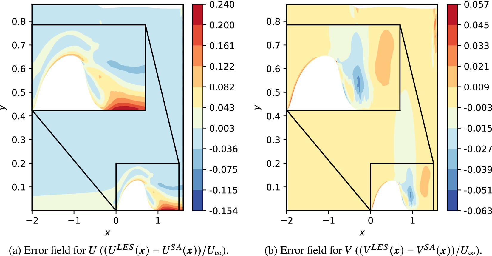


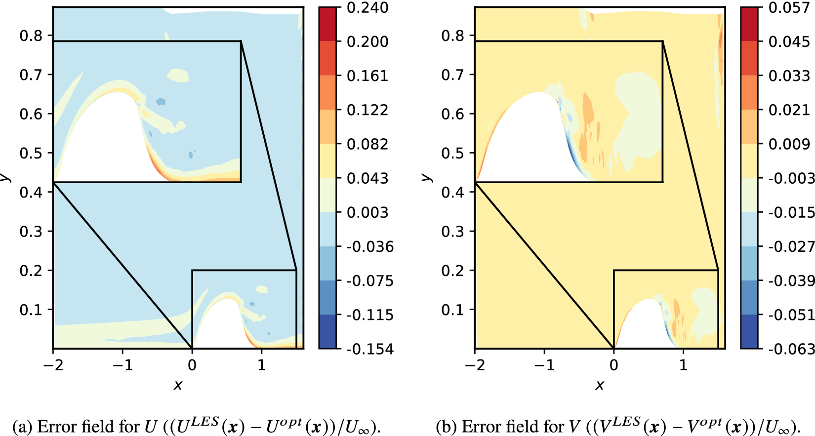


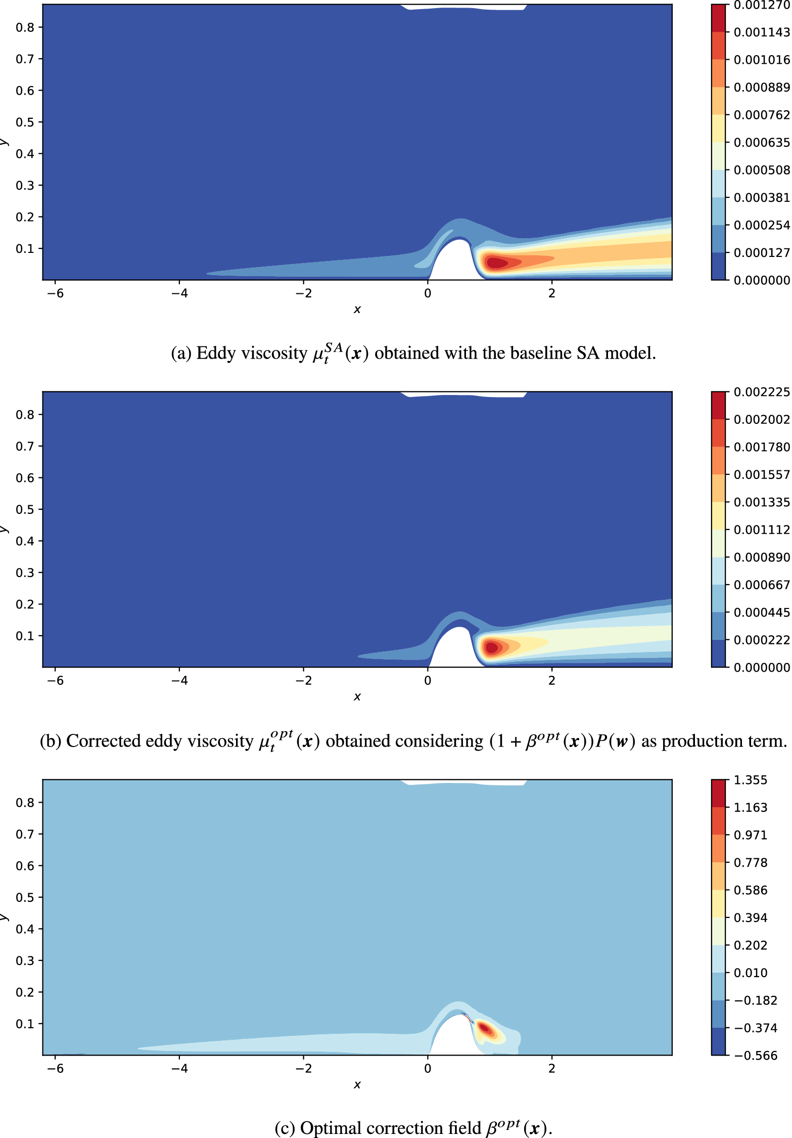

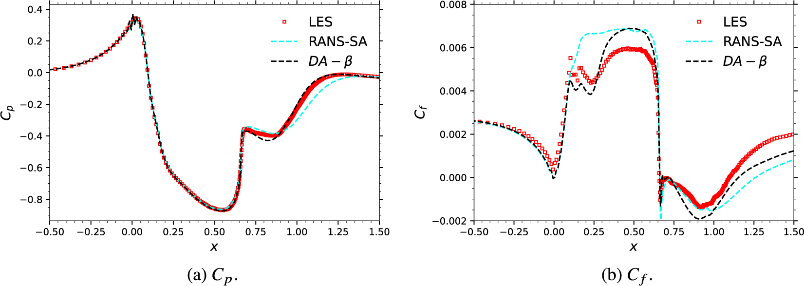


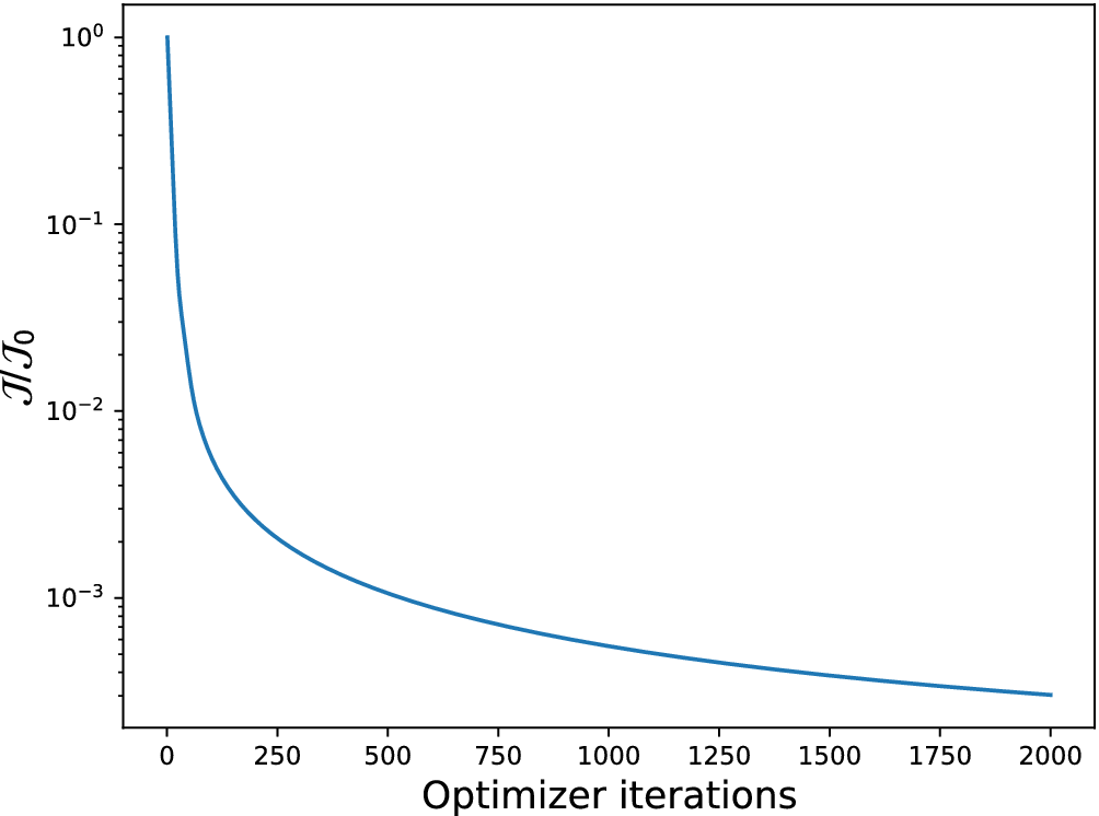


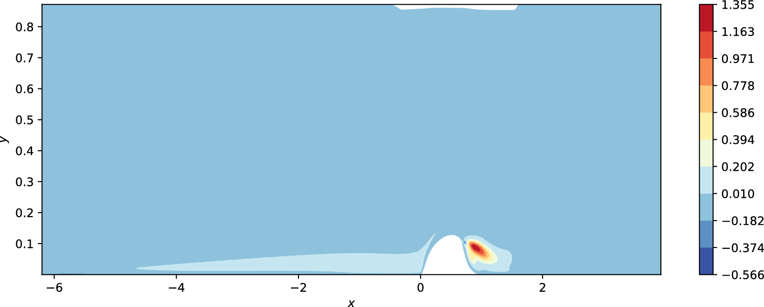


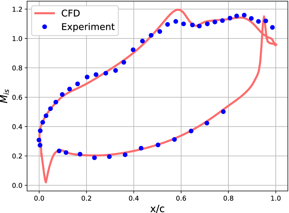


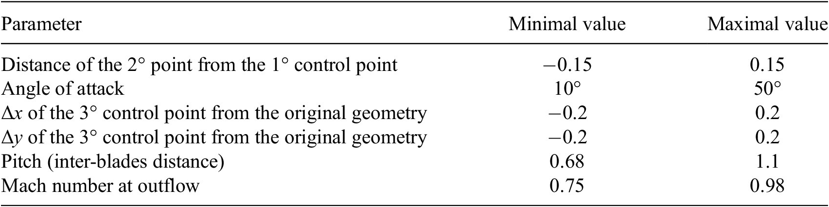


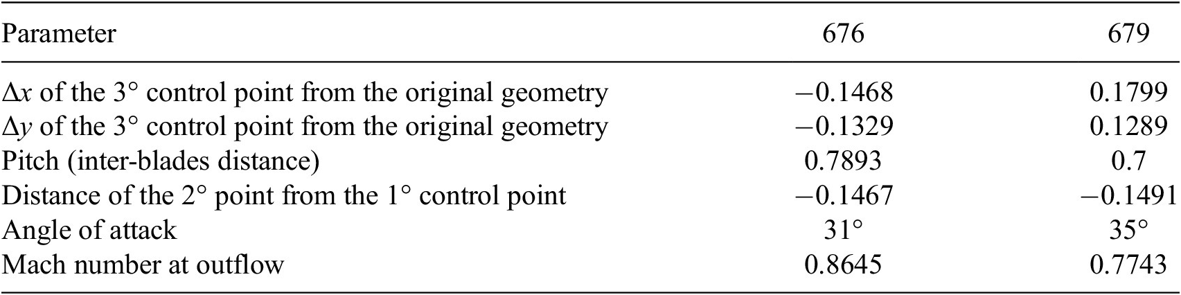


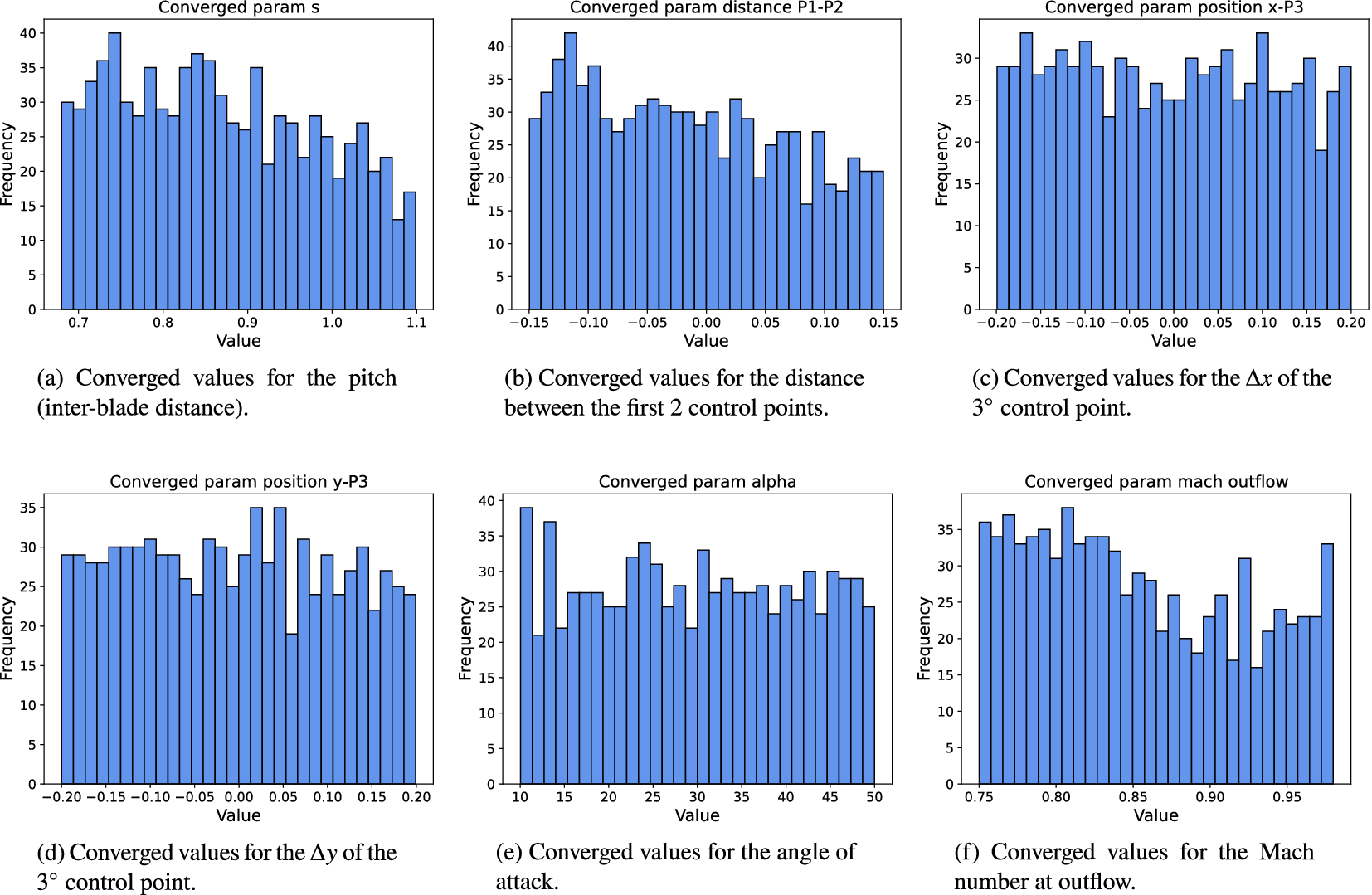
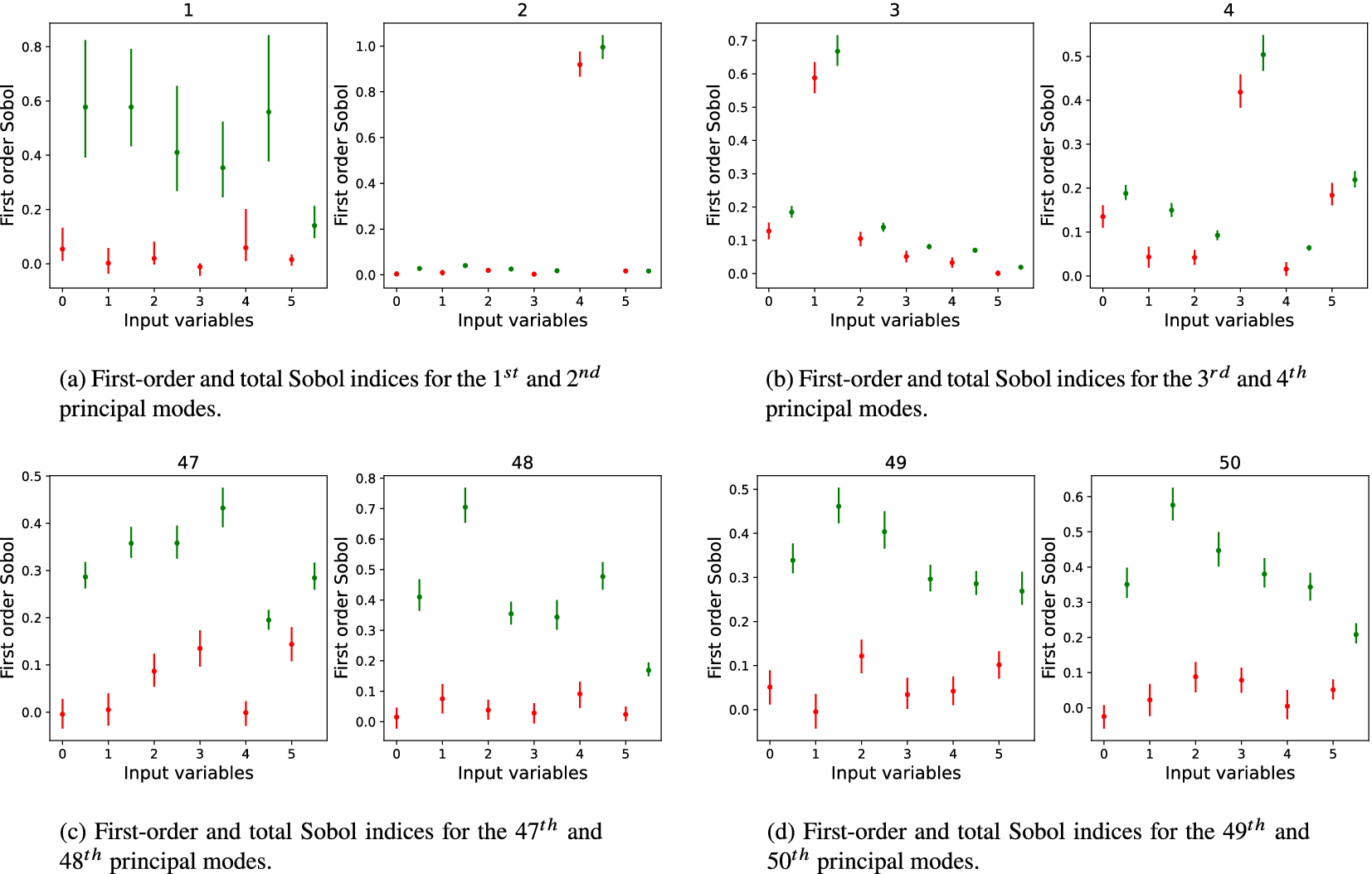



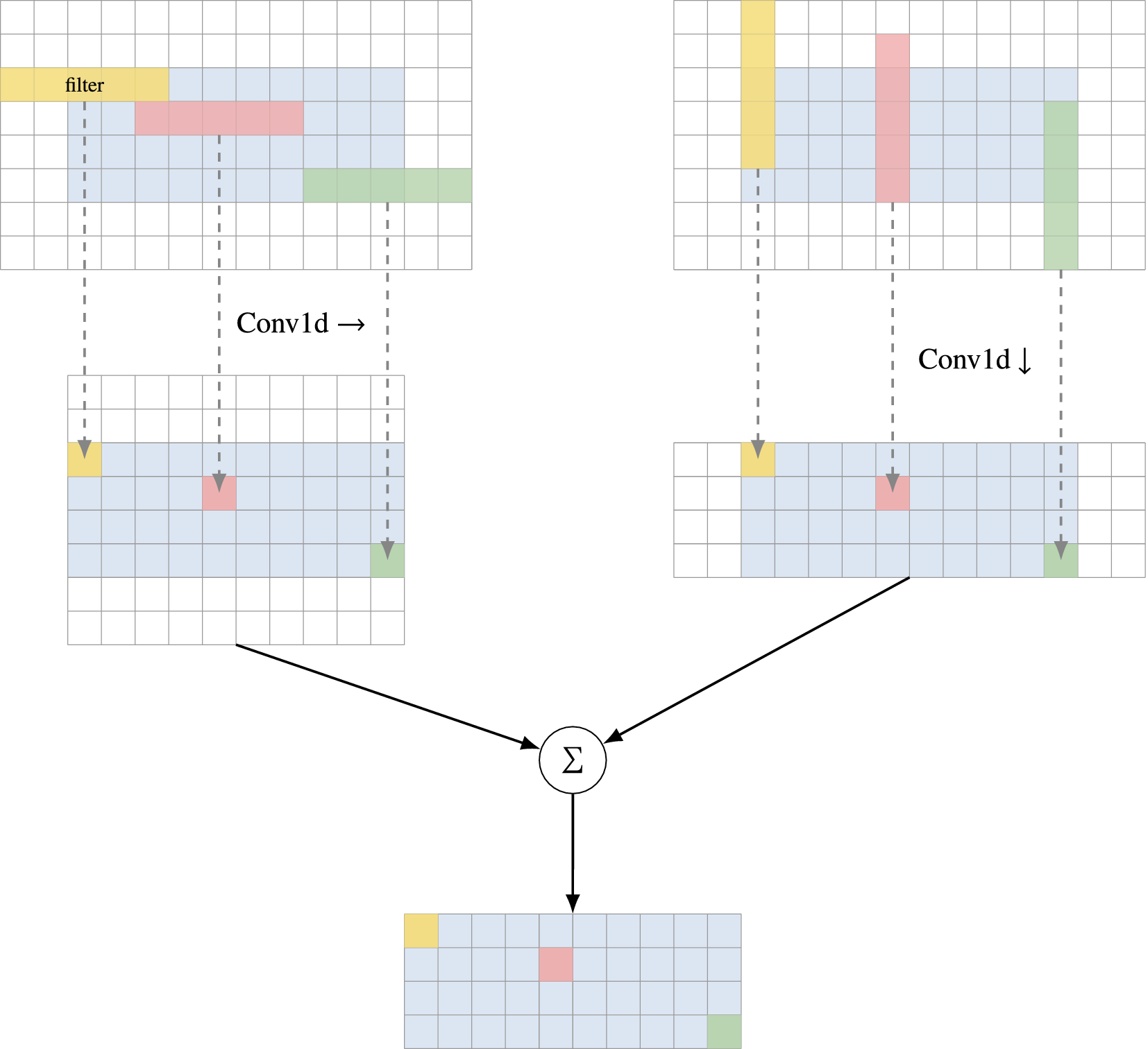

 Open access


Comments
No Comments have been published for this article.